Adjusting for Spatial Effects in Genomic Prediction

Abstract

This paper investigates the problem of adjusting for spatial effects in genomic prediction. Despite being seldomly considered in genomic prediction, spatial effects often affect phenotypic measurements of plants. We consider a Gaussian random field model with an additive covariance structure that incorporates genotype effects, spatial effects and subpopulation effects. An empirical study shows the existence of spatial effects and heterogeneity across different subpopulation families, while simulations illustrate the improvement in selecting genotypically superior plants by adjusting for spatial effects in genomic prediction.

Keywords: Gaussian random field; Genomic prediction; Spatial effects; Subpopulation effects.

1 Introduction

In plant breeding, predicting the genetic value of plant genotypes plays an important role in determining which genotypes to include in subsequent generations. Recently, several powerful statistical methods have been developed that use high-dimensional single-nucleotide polymorphism (SNP) genotypes for genomic prediction. Most of the methods based on mixed linear models (MLM) are quite flexible due to the consideration of fixed and random effects. For instance, population structure (discussed in Pritchard et al. 2000) is often accounted for by modeling the fixed effects of principal components (PCs) derived from the SNPs (Price et al., 2006; Reich et al., 2008; McVean, 2009). For unified MLM approaches (Yu et al., 2006), SNP data are used to determine a kinship matrix that is assumed to be proportional to the variance of a vector of random effects that accounts for dependencies due to relatedness among individuals. For a more computationally efficient compressed MLM (CMLM) approach (Zhang et al., 2010), data from many individuals are compressed into a smaller number of groups, and the interindividual kinship matrix is replaced by a lower-dimensional matrix that characterizes correlations among group random effects induced by genetic similarities among groups.

Aside from correlations due to relatedness among individuals or groups, phenotypes measured on plants grown in fields can be spatially correlated (Stroup, 2002). Such correlation can arise because plants growing near each other may share a common microenvironment that differs from the microenvironment experienced by plants in other parts of the field. This microenvironmental variation can induce phenotypic similarity among neighboring plants. When such spatial effects exist but are unaccounted for in the analysis, decisions about which plant genotypes are expected to perform best with regard to one or more phenotypic traits can be adversely affected. With the adjustment of these effects, some high-throughput phenotyping technologies (Cabrera-Bosquet et al., 2012; Masuka et al., 2012; White et al., 2012) can be applied to increase plant yields.

Several works (Stroup and Mulitze, 1991; Stroup et al., 1994; Gilmour et al., 1997; Crossa et al., 2006; Lado et al., 2013; Bernal-Vasquez et al., 2014; Selle et al., 2019) have considered spatial effects in linear mixed-effects models. Gilmour et al. (1997) proposed a separable autoregressive (AR$\times$AR) model. As suggested by Bernal-Vasquez et al. (2014), fitting a row and column model (RC) (i.e., a model with an effect for each row and for each column in a field experiment layout) can account for a substantial portion of phenotypic heterogeneity that may be due to spatial effects. Lado et al. (2013) compared RC models with approaches that attempt to adjust for spatial effects by using the difference between a plot’s response value and the average response of its neighboring plots as a covariate. Such a method, referred to by Lado et al. (2013) as “moving-means as a covariate” (MVNG), was found to best fit the data and lead to the most accurate phenotypic predictions. Selle et al. (2019) considered a Bayesian framework to model the spatial mixed-effects. In addition, several smoothing methods (Verbyla et al., 1999; Durban et al., 2003; Rodriguez-Alvarez et al., 2018) are developed to model the spatial trends more explicitly. In particular, Rodriguez-Alvarez et al. (2018) used a smooth bivariate surface (SpATS) to model the random spatial effects which captures both large-scale and small-scale dependences. In this paper, we propose an alternative modeling strategy that has some conceptual advantages because it integrates information from high-dimensional markers, spatial locations and subpopulation structure via Gaussian kernels and provides competing or better performance than several existing approaches for spatial adjustments in genomic prediction.

We study two datasets. One is a maize dataset involving a nested association mapping (NAM) panel consisting of 4660 recombinant inbred lines (RILs) derived from crosses between a reference inbred line B73 and 25 other founder inbreds. More information about the NAM panel is available in Yu et al. (2008) and at http://www.panzea.org. The RILs derived by crossing B73 to any one of the 25 other founders from a subpopulation of RILs. Thus, the 4660 RILs we consider can be partitioned into 25 subpopulations. Even after conditioning on SNP genotypes carried by each RIL, phenotypic responses from RILs within a subpopulation are expected to be more strongly correlated than responses from RILs in different subpopulations. This within-subpopulation correlation is expected due to shared genetic material as well as characteristics of the experimental design described in Section 2. The second dataset is a wheat dataset which consists of genotype and phenotype data on 384 advanced lines from two different breeding programs. The data are provided in Lado et al. (2013).

The goal of this paper is to predict the genetic value of each maize RIL or each wheat line from a huge number of SNP marker genotypes, while accounting for the genetic and spatial dependence among phenotypic measurements. We focus on a Gaussian random field (GRF) model with an additive covariance matrix structure that incorporates genotype effects, spatial effects and subpopulation effects. For genotype effects, we adopt a Gaussian kernel (Morota et al., 2013; Ober et al., 2011) to capture general relationships between genotypes and phenotypes. We compare our spatially adjusted genomic predictions with genomic predictions generated by a design-based incomplete block (IB) linear mixed-effects model and existing methods CMLM (Zhang et al., 2010), RC (Bernal-Vasquez et al., 2014), MVNG (Lado et al., 2013) and SpATS (Rodriguez-Alvarez et al., 2018). In a simulation study presented in Section 5, we apply the proposed GRF method to help identify the best plant genotypes.

The rest of the paper is organized as follows. Real data are described in Section 2. The proposed GRF is constructed in Section 3. Within Section 3, we also discuss kernels and corresponding parameter estimation methods. Numerical performances of the proposed method for genomic predictions and for choosing the best plant genotypes are illustrated in an empirical study in Section 4 and a simulation study in Section 5, respectively. The paper concludes with a discussion in Section 6. Some supplementary materials are provided in Section S1.

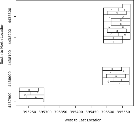
Figure 1: Geographic locations of 25 subpopulations labeled A through Y.

2 Data

Throughout this paper, we used Data1 to refer to a maize NAM RIL dataset comprised of 4660 RILs genotyped at $687,869$ SNP markers. The phenotypic value for each RIL is a measurement of the carbon dioxide ($\text{CO}_{2}$) emitted from plant material incorporated in a soil sample. Scientific interest centers on identifying RILs whose genetic constitution makes them relatively low emitters of $\text{CO}_{2}$.

The 4660 RILs in Data1 can be partitioned into 25 subpopulations, each produced from a biparental cross of inbred line B73 to one of the 25 NAM founder inbred lines. A side-by-side box plot to compare the carbon dioxide emissions among these 25 subpopulations is available in Figure S1 of the supplemental document. Due to the large number of RILs and limited field plot availability, the experimental design is unreplicated with a single plot for each RIL distributed across three nearby agricultural fields, with no two plots separated by more than 2.5 miles. RILs from any given subpopulation were randomized to plots within a single subpopulation-specific region (as depicted in Figure 1) to facilitate mapping of quantitative trait loci separately for each subpopulation. In our combined analysis of data from all RILs, we expect correlations among the phenotypic values for RILs within each subpopulation due to both region and subpopulation effects, as well as spatially correlated plot effects, which induce correlations among phenotypic values within any field regardless of subpopulation membership.

Our second dataset (henceforth labeled Data2) is the 2011 wheat dataset presented in Lado et al. (2013). This dataset contains results for 384 wheat lines genotyped at 102324 biallelic markers and phenotyped for grain yield (GY), thousand kernel weight (TKW), the number of kernels per spike (NKS), and days to heading (DH) under two levels of water supply: mild water stress (MWS) and fully irrigated (FI). For both MWS and FI, the 384 wheat lines were planted in an alpha-lattice design with $20$ incomplete blocks of size 20 and two complete replications. Within each replications, 382 genotypes were planted on one plot each, while 2 of the 384 genotypes were planted on 9 plots each to cover all $20\times 20$ plots. Lado et al. (2013) also analyzed data collected in 2012 from two separate locations, but the 2012 data contain measurements of only the grain yield phenotype. We restrict our analysis to the 2011 data only to simplify our presentation. The same dataset has been analyzed by Rodriguez-Alvarez et al. (2018) and Selle et al. (2019).

3 Methods

3.1 Models

We are given a training dataset $\{y_{i},\bm{x}_{i},b_{i},\bm{s}_{i}\}_{i=1}^{n}$, where $y_{i}\in\mathbb{R}$ represents a phenotype measurement, $\bm{x}_{i}\in\mathcal{X}$ is the corresponding $p$-dimensional vector of binary marker genotypes, $b_{i}\in\mathcal{B}$ is the corresponding subpopulation family index of the observation and $\bm{s}_{i}\in\mathcal{S}$ is the corresponding spatial location of the observation. Here, $\mathcal{X}$, $\mathcal{B}$ and $\mathcal{S}$ represent the sets of possible values of binary marker genotype vectors, subpopulation family indices and spatial locations, respectively.

We propose a Gaussian random field (GRF) approach that carefully models (i) genotype effects, (ii) subpopulation effects and (iii) spatial effects. More specifically, for $i=1,\ldots,n$, suppose

$$y_{i}=\mathbb{Z}\left(\bm{t}_{i}\right)+\epsilon_{i},$$ (1)

where $\bm{t}_{i}=(\bm{x}^{\intercal}_{i},b_{i},\bm{s}^{\intercal}_{i})^{\intercal}$, $\mathbb{Z}(\bm{t}_{i})$ is an observation at $\bm{t}_{i}$ of a GRF $\mathbb{Z}$ defined over index domain $\mathcal{T}=\mathcal{X}\times\mathcal{B}\times\mathcal{S}$, and $\epsilon_{i}$ is a mean-zero Gaussian random variable independent of $\mathbb{Z}$. Further, we let $\bm{\epsilon}=(\epsilon_{1},\ldots,\epsilon_{n})^{\intercal}$ and assume $\mathrm{Var}(\bm{\epsilon})=\sigma_{\epsilon}^{2}\bm{I}_{n\times n}$ with $\bm{I}_{n\times n}$ being the identity matrix of size $n$. We assume a constant mean function for $\mathbb{Z}$, i.e., $\mathbb{E}(\mathbb{Z}(\bm{t}))=\mu$ for any $\bm{t}\in\mathcal{T}$. The power of this model lies in the flexible modeling of the covariance structure of $\mathbb{Z}$.

We consider an additive model for the covariance function that accounts for the three major effects. Specifically, for any $\bm{t}_{i}=(\bm{x}_{i}^{\intercal},b_{i},\bm{s}_{i}^{\intercal})^{\intercal},\bm{t}_{k}=(\bm{x}_{k}^{\intercal},b_{k},\bm{s}_{k}^{\intercal})^{\intercal}\in\mathcal{T}=\mathcal{X}\times\mathcal{B}\times\mathcal{S}$, we assume

$$\text{Cov}[\mathbb{Z}(\bm{t}_{i}),\mathbb{Z}(\bm{t}_{k})]=C\left(\bm{t}_{i},\bm{t}_{k}\right)=\sigma_{g}^{2}C_{g}\left(\bm{x}_{i},\bm{x}_{k}\right)+\sigma_{b}^{2}C_{b}\left(b_{i},b_{k}\right)+\sigma_{s}^{2}C_{s}\left(\bm{s}_{i},\bm{s}_{k}\right),$$

where $\sigma_{g}^{2}$, $\sigma_{b}^{2}$ and $\sigma_{s}^{2}$ are variance components and $C_{g}:\mathcal{X}^{2}\to\mathbb{R}$, $C_{b}:\mathcal{B}^{2}\to\mathbb{R}$ and $C_{s}:\mathcal{S}^{2}\to\mathbb{R}$ are unit-diagonal kernel functions that quantify the corresponding dependence structures arising from similarity among observations with respect to genetic markers, subpopulations and spatial locations, respectively. Equivalently, we assume that the GRF $\mathbb{Z}$ can be decomposed into $\mathbb{Z}(\bm{t}_{i})=\mu+\mathbb{Z}_{g}(\bm{x}_{i})+\mathbb{Z}_{b}(b_{i})+\mathbb{Z}_{s}(\bm{s}_{i})$, where $\mathbb{Z}_{g}$, $\mathbb{Z}_{b}$, $\mathbb{Z}_{s}$ are mean-zero Gaussian random fields with covariance structures determined by $\sigma_{g}^{2}{C}_{g}$, $\sigma_{b}^{2}{C}_{b}$ and $\sigma_{s}^{2}{C}_{s}$, respectively. We quantify the strength of spatial effects relative to the effects associated with marker genotypes by the variance component ratio $\gamma=\sigma_{s}^{2}/\sigma_{g}^{2}$.

3.2 Marker Kernel $C_{g}$

Following Morota and Gianola (2014) and references therein, we choose the Gaussian kernel

$$C_{g}\left(\bm{x}_{i},\bm{x}_{k}\right)=\exp\left(-\frac{\|\bm{x}_{i}-\bm{x}_{k}\|^{2}}{\tau}\right),\text{ for any }\bm{x}_{i},\bm{x}_{k}\in\mathcal{X}$$

where $\|\cdot\|$ represents the Euclidean norm and $\tau$ is a parameter greater than zero.

Compared with other common kernels, the Gaussian kernel has been empirically shown to give robust and strong predictive performance. In Ober et al. (2011), the more general Matérn kernel is studied, but the Gaussian kernel performed best among the Matérn family based on their simulation study. Since the marker genotypes take discrete values, there is a temptation to choose a kernel on discrete index space. In Morota et al. (2013), a discretized Gaussian kernel, referred to as a diffusion kernel, was applied to dairy and wheat data for predicting phenotypes using marker information. However, the predictive power of such a kernel was similar to the Gaussian kernel.

Current high-throughput genotyping technology can provide genotype calls for hundreds of thousands of SNPs. Since most SNPs are unassociated with phenotype or conditionally unassociated with phenotype given other SNPs, $C_{g}(\bm{x}_{i},\bm{x}_{k})$ does not necessarily provide a good representation of correlation between the $i$-th and $k$-th lines when all SNPs are included in the vector of marker genotypes. To reduce computation time and improve genomic prediction, we use $\mathrm{FarmCPU}$ (Liu et al., 2016) to select important SNPs for inclusion in $\bm{x}_{i}$ rather than using the entire ensemble of SNPs. The details of our SNP selection procedure are discussed in Section S1 of the supplementary material.

3.3 Subpopulation Kernel $C_{b}$

The subpopulation GRF $\mathbb{Z}_{b}$ is motivated by genetic heterogeneity across different subpopulations and genetic similarity within subpopulations that may not be fully captured by SNP genotypes. We consider $C_{b}(b_{i},b_{k})=\mathds{1}(b_{i}=b_{k})$ for any $b_{i},b_{k}\in\mathcal{B}$, where $\mathds{1}(\cdot)$ is the indicator function. This covariance structure is equivalent to that induced by a model with independent, constant-variance subpopulation random effects.

3.4 Spatial Kernel $C_{s}$

In an agricultural field trial, plots are typically embedded in a regular rectangular array with say $m_{1}$ rows and $m_{2}$ columns. To adjust for spatial effects that may exist in such trials, the class of spatial autoregressions on regular rectangular lattice has been quite popular following the works of Besag and Green (1993); Besag et al. (1995); Besag and Higdon (1999); Dutta and Mondal (2015) and Mondal et al. (2020). In this work we focus on the class of stationary autoregressions with modification described as follows. Consider a bigger array with $m_{1}^{\prime}=m_{1}+4$ rows and $m_{2}^{\prime}=m_{2}+4$ columns obtained by adding two virtual plots (Besag and Higdon, 1999) to each boundary to reduce the boundary effects. Suppose that for any positive integer $k,$ $\bm{W}_{k}$ denotes the $k\times k$ matrix with

$$W_{k}(1,1)=W_{k}(k,k)=1,~{}W_{k}(i,i)=2(1<i<k),~{}W_{k}(i,i+1)=W_{k}(i+1,i)=-\mathds{1}(1\leq i<k),$$

and $W_{k}(i,j)=0$ otherwise. Here, $W_{k}(i,j)$ represents the $(i,j)$-th entry of $\bm{W}_{k}$. Next define $\bm{N}_{01}=\bm{I}_{m_{2}^{\prime}}\otimes\bm{W}_{m_{1}^{\prime}}$, $\bm{N}_{10}=\bm{W}_{m_{2}^{\prime}}\otimes\bm{I}_{m_{1}^{\prime}}$, and

$$\bm{W}=\beta_{00}\bm{I}+\beta_{01}\bm{N}_{01}+\beta_{10}\bm{N}_{10},$$

where $\beta_{00}$, $\beta_{01}$ and $\beta_{10}$ are positive parameters with the identifiability constraint $\beta_{00}+2(\beta_{01}+\beta_{10})=1.$ Let $\bm{D}$ be the diagonal matrix consisting of the diagonal entries of $\bm{W}^{-1}.$ Next, for any plot $s_{i}$ suppose $\bm{h}_{i}=\bm{h}(s_{i})$ denotes the incidence vector of length $m_{1}^{\prime}m_{2}^{\prime}$. That is, the $j$-th entry of $\bm{h}_{i}$ is 1 if and only if $s_{i}$ corresponds to the $j$th plot in the $m_{1}^{\prime}\times m_{2}^{\prime}$ array where the plots in the array are enumerated in a column major format; the rest of the entries of $\bm{h}_{i}$ are zeros.

Finally, the spatial covariance of $\left(\mathbb{Z}_{s}(s_{1}),\ldots,\mathbb{Z}_{s}(s_{n})\right)^{\intercal}$ is given by

$$\sigma_{s}^{2}C_{s}(s_{i},s_{j})=\sigma^{2}_{s}\bm{h}_{i}^{\intercal}\bm{D}^{-1/2}\bm{W}^{-1}\bm{D}^{-1/2}\bm{h}_{j},$$

where $\sigma^{2}_{s}$ is the spatial variance component introduced in Section 3. The advantage of this spatial kernel is that it makes the marginal variances at observed plots constant, while keeping the pairwise correlations the same as those that would be obtained from the stationary autoregression covariance matrix $\bm{W}^{-1}$. However, note that the weights on the neighbors are no longer $\beta_{01}$ and $\beta_{10}$ but are approximately proportional to them at the interior plots because the variances at the interior plots are approximately constant (Besag and Kooperberg, 1995).

The anisotropy parameters $\beta_{01}$ and $\beta_{10}$ play an important role because these parameters are related to the field geometry. In fact, McCullagh and Clifford (2006) found substantial empirical evidence that the non-anthropogenic variability in field trials can be explained by an isotropic spatial process with correlation decaying approximately logarithmically with distance. This would imply, for example, that for square plots the values of $\beta_{01}$ and $\beta_{10}$ should be approximately equal. On the other hand, if the plots are rectangular and the spacing between the plots is negligible compared with the plot sizes, the ratio of the $\beta_{01}$ and $\beta_{10}$ should be close to the aspect ratio of the plots. Also if the design is single column replication (see the El Batán trial in Besag and Higdon (1999)), then $\beta_{10}$ is zero. In practice the estimates of $\beta_{01}$ and $\beta_{10}$ are automatically adjusted to the plot geometry and the interplot spacing. For Data1, in our context, the spatial layout in the maize experiment mimics a single–column replicate design because the distance between two east–west neighboring maize plants is much larger than the distance between two north–south neighbors. Thus, we apriori expect the estimate of $\beta_{10}\approx 0$. This expectation is corroborated by the ML estimates in Section 4.2, where we see that the MLE of $\beta_{10}$ occurs at the boundary. On the other hand, the plots in the Data2 are rectangular, and the interplot spacings are not very large. Thus, we expect the MLE of $\beta_{10}$ and $\beta_{01}$ to be somewhere between $0$ and $0.5$ and this is corroborated by the estimates in Section 4.3.

The parameter $\beta_{00}$, on the other hand, controls the strength of the neighboring correlations and the range of the correlation. Interestingly, the boundary value of $\beta_{00}=0$ gives rise to an intrinsic autoregression process and is the focus of Besag et al. (1995), Besag and Higdon (1999) and Dutta and Mondal (2015) in the context of fertility adjustments in agricultural variety trials. In particular, the foundational work of McCullagh and Clifford (2006) and empirical evidence from Besag et al. (1995), Besag and Higdon (1999) and Dutta and Mondal (2015, 2016) advocate the use of the intrinsic model for spatial adjustments in agricultural trials. Consequently, to build a proper covariance model and to avoid boundary issues in maximum likelihood estimation, we fix the parameter $\beta_{00}$ at a small value. To that end, following the suggestion in Besag and Kooperberg (1995), we numerically compute the neighboring correlations for various values of $\beta_{00}$ (with $\beta_{01}=\beta_{10}$ = $(1-\beta_{00})/2)$. We observe that the theoretical neighboring correlation changes by 11.26% when $\beta_{00}$ changes from $0.01$ to $0.001$ and only by 1.69% when the $\beta_{00}$ changes from $0.001$ to $0.0001$. A similar conclusion is obtained where $\beta_{01}$ is held fixed at other values including $0$ and $0.5$. Because a change of 1.69% in neighboring correlation is practically negligible, we choose to fix the value of $\beta_{00}$ at $0.001$. Our analyses (see supplementary materials Table S3) also shows that the prediction accuracies and ranking do not change appreciably by changing $\beta_{00}$ from $0.001$ to $0.0001$.

We end this section with references to other commonly used spatial kernels in such prediction problems. Rather than using the autoregression models to fit the spatial effects, several works (Crossa et al., 2006; Lado et al., 2013; Bernal-Vasquez et al., 2014) considered them as random effects in simple mixed linear models. In the context of agricultural field trials, Gleeson and Cullis (1987), Cullis and Gleeson (1991), Zimmerman and Harville (1991), Gleeson and Cullis (1987), Gilmour et al. (1997) and Cullis et al. (1998) developed elaborate model for adjusting for systematic and non-systematic trends. Their spatial adjustment models, despite drawing criticism for their heavy dependence on the coordinate system by McCullagh and Clifford (2006), have been quite effective in practice for spatial adjustments and may be potential alternatives for spatial adjustments in genomic prediction.

3.5 Estimation

For the training dataset $\{y_{i},\bm{x}_{i},b_{i},\bm{s}_{i}\}_{i=1}^{n}$, let $\bm{C}$ be the $n\times n$ matrix with element $i,j$ equal to $C(\bm{t}_{i},\bm{t}_{j})$ for all $i,j=1,\ldots,n$. Define $\bm{C}_{g}$, $\bm{C}_{b}$ and $\bm{C}_{s}$ analogously. Then, the covariance matrix of the vector of $n$ phenotypic response values $\bm{y}=(y_{1},\ldots,y_{n})^{\intercal}$ can be written as

$$\bm{\Sigma}=\bm{C}+\sigma_{\epsilon}^{2}\bm{I}_{n\times n}=\sigma_{g}^{2}\bm{C}_{g}+\sigma_{b}^{2}\bm{C}_{b}+\sigma_{s}^{2}\bm{C}_{s}+\sigma_{\epsilon}^{2}\bm{I}_{n\times n}.$$

The variance–covariance matrix $\bm{\Sigma}$ is a function of the parameters $\sigma_{g}$, $\tau$, $\sigma_{b}$, $\sigma_{s}$ and $\sigma_{\epsilon}$. We maximize the log-likelihood to estimate these five parameters simultaneously.

It is straightforward to show that, for any given value of $\bm{\Sigma}$, the likelihood is maximized over $\mu$ at $\widehat{\mu}=\bm{1}^{T}\bm{\Sigma}^{-1}\bm{y}/\bm{1}^{T}\bm{\Sigma}^{-1}\bm{1}$. Thus, the corresponding profile log-likelihood function is

$$\ell\left(\sigma_{g},\tau,\sigma_{b},\sigma_{s},\sigma_{\epsilon}\right)=-\frac{1}{2}\log|\bm{\Sigma}|-\frac{\left(\bm{y}-\widehat{\mu}\bm{1}\right)^{T}\bm{\Sigma}^{-1}\left(\bm{y}-\widehat{\mu}\bm{1}\right)}{2}.$$

Finding maximizers of this profile log-likelihood function yields maximum likelihood estimates (MLEs) $\widehat{\sigma}_{g},\widehat{\tau},\widehat{\sigma}_{b},\widehat{\sigma}_{s}$, and $\widehat{\sigma}_{\epsilon}$. Let $\widehat{\bm{C}}_{g}$ and $\widehat{\bm{\Sigma}}$ be the estimates of the covariance structures $\bm{C}_{g}$ and $\bm{\Sigma}$ obtained by replacing the unknown parameters with their MLEs.

Considering the joint distribution of $\bm{y}$, $\bm{Z}_{g}=(\mathbb{Z}_{g}(\bm{x}_{1}),\ldots,\mathbb{Z}_{g}(\bm{x}_{n}))^{\intercal}$, $\bm{Z}_{b}=(\mathbb{Z}_{b}(b_{1}),\ldots,\mathbb{Z}_{b}(b_{n}))^{\intercal}$ and $\bm{Z}_{s}=(\mathbb{Z}_{s}(\bm{s}_{1}),\ldots,\mathbb{Z}_{s}(\bm{s}_{n}))^{\intercal}$, we have

$${\small\begin{bmatrix}\bm{y}\\ \bm{Z}_{g}\\ \bm{Z}_{b}\\ \bm{Z}_{s}\end{bmatrix}\sim\mathcal{N}\left(\begin{bmatrix}\mu\bm{1}\\ \bm{0}\\ \bm{0}\\ \bm{0}\end{bmatrix},\begin{bmatrix}\bm{\Sigma}&\sigma_{g}^{2}\bm{C}_{g}&\sigma_{b}^{2}\bm{C}_{b}&\sigma_{s}^{2}\bm{C}_{s}\\ \sigma_{g}^{2}\bm{C}_{g}&\sigma_{g}^{2}\bm{C}_{g}&\bm{0}&\bm{0}\\ \sigma_{b}^{2}\bm{C}_{b}&\bm{0}&\sigma_{b}^{2}\bm{C}_{b}&\bm{0}\\ \sigma_{s}^{2}\bm{C}_{s}&\bm{0}&\bm{0}&\sigma_{s}^{2}\bm{C}_{s}\end{bmatrix}\right).}$$

Based on our MLEs, we can estimate the conditional mean and conditional variance of $\bm{Z}_{g}$, $\bm{Z}_{b}$ and $\bm{Z}_{s}$ given $\bm{y}$, by

$$\widehat{\mathbb{E}}\left(\left.\begin{bmatrix}\bm{Z}_{g}\\ \bm{Z}_{b}\\ \bm{Z}_{s}\end{bmatrix}\right|\bm{y}\right)=\begin{bmatrix}\bm{0}\\ \bm{0}\\ \bm{0}\end{bmatrix}+\begin{bmatrix}\widehat{\sigma}_{g}^{2}\widehat{\bm{C}}_{g}\\ \widehat{\sigma}_{b}^{2}\bm{C}_{b}\\ \widehat{\sigma}_{s}^{2}\bm{C}_{s}\end{bmatrix}\widehat{\bm{\Sigma}}^{-1}(\bm{y}-\widehat{\mu}\bm{1})$$ (2)

and

$$\widehat{\mathrm{Var}}\left(\left.\begin{bmatrix}\bm{Z}_{g}\\ \bm{Z}_{b}\\ \bm{Z}_{s}\end{bmatrix}\right|\bm{y}\right)=\begin{bmatrix}\widehat{\sigma}_{g}^{2}\widehat{\bm{C}}_{g}&0&0\\ 0&\widehat{\sigma}_{b}^{2}\bm{C}_{b}&0\\ 0&0&\widehat{\sigma}_{s}^{2}\bm{C}_{s}\end{bmatrix}-\begin{bmatrix}\widehat{\sigma}_{g}^{2}\widehat{\bm{C}}_{g}\\ \widehat{\sigma}_{b}^{2}\bm{C}_{b}\\ \widehat{\sigma}_{s}^{2}\bm{C}_{s}\end{bmatrix}\widehat{\bm{\Sigma}}^{-1}\begin{bmatrix}\widehat{\sigma}_{g}^{2}\widehat{\bm{C}}_{g}&\widehat{\sigma}_{b}^{2}\bm{C}_{b}&\widehat{\sigma}_{s}^{2}\bm{C}_{s}\end{bmatrix}.$$ (3)

4 Empirical Study

4.1 Existing Methods

For the purpose of benchmarking, we compared our method with methods based on the Compressed Mixed Linear Model (CMLM) (Zhang et al., 2010) implemented in the R package GAPIT (Lipka et al., 2012), the Row and Column Model (RC) (Bernal-Vasquez et al., 2014), the linear regression with moving means as covariable model (MVNG) (Lado et al., 2013) and Spatial Analysis of field Trials with Splines (SpATS) implemented in the R package SpATS (Rodriguez-Alvarez et al., 2018). These competing methods are described in the following. All the methods are implemented in R language.

Compressed Mixed Linear Model

Let $\bm{M}$ be a matrix whose columns correspond to the first few principal components (usually 3 or 5 by default) computed from the binary genotype matrix to represent population structure. The compressed mixed linear model is

$$\bm{y}=\mu\bm{1}+\bm{M}\bm{\beta}+\bm{Z}\bm{\bar{u}}+\bm{e},$$

where $\bm{\bar{u}}_{r\times 1}\sim\mathcal{N}(\bm{0},\sigma_{\bar{u}}^{2}\bm{\bar{K}}_{r\times r})$ represents an unknown vector of random additive genetic effects and $\bm{e}\sim\mathcal{N}(\bm{0},\sigma_{e}^{2}\bm{I})$ is the unobserved vector of errors. The random effects in $\bm{\bar{u}}_{r\times 1}$ are intended to represent the effects of multiple background quantitative trait loci (QTL) on the phenotypic response values. Note that $\bm{\bar{u}}_{r\times 1}$ is of dimension $r\times 1$ rather than $n\times 1$ as in the MLM because that $\bm{\bar{u}}_{r\times 1}$ represents different groups $t=1,\ldots,r$ clustered according to a full kinship matrix $\bm{K}_{n\times n}$ rather than individuals/lines. Meanwhile, the matrix $\bm{\bar{K}}_{r\times r}$ is the corresponding kinship matrix that accounts for varying degrees of genetic similarity among groups rather than among individuals/lines. We adopt the formula for the full kinship matrix suggested by VanRaden (2008):

$$\bm{K}_{n\times n}=\frac{\widetilde{\bm{X}}^{(g)}\widetilde{\bm{X}}^{(g)\intercal}}{\sum_{i}2p_{i}(1-p_{i})},$$ (4)

where $\widetilde{\bm{X}}^{(g)}$ contains allele calls centered so that each row sums to zero and $p_{i}$ is the frequency of the minor allele at locus $i$. As for the group kinship matrix $\bm{\bar{K}}_{r\times r}=(\bar{K}_{st})$ where $s,t=1$ to $r$, each of the entry $\bar{K}_{st}$ is defined as the average of a set of $\{K_{hj}\}$ where $h$ belongs to group $s$ and $j$ belongs to group $t$. For the maize dataset Data1, the Bayesian information criterion (Zhang et al., 2010) selects no principal components in the matrix $\bm{M}$. For the wheat dataset Data2, we considered one, three, five and ten principal components for $\bm{M}$. We found no important difference, and thus, we adopted the default setting with the first three principal components in $\bm{M}$.

Incomplete Block Model

Motivated by the alpha-lattice experimental design underlying the wheat dataset, we also consider an incomplete block (IB) model defined as follows. Using the same principal component matrix $\bm{M}$ in CMLM, the IB model assumes

$$\bm{y}=\mu\bm{1}+\bm{M}\bm{\beta}+\bm{Z}_{\bm{u}_{g}}\bm{u}_{g}+\bm{Z}_{\bm{u}_{\text{rep}}}\bm{u}_{\text{rep}}+\bm{Z}_{\bm{u}_{\text{bl(rep)}}}\bm{u}_{\text{bl(rep)}}+\bm{e},$$

where $\bm{u}_{g}\sim\mathcal{N}(\bm{0},\sigma_{g}^{2}\bm{K})$, $\bm{u}_{\text{rep}}\sim\mathcal{N}(\bm{0},\sigma_{\text{rep}}^{2}\bm{I})$, $\bm{u}_{\text{bl(rep)}}\sim\mathcal{N}(\bm{0},\sigma_{\text{bl(rep)}}^{2}\bm{I})$ and $\bm{e}\sim\mathcal{N}(\bm{0},\sigma_{e}^{2}\bm{I})$ represent independent, unknown vectors of additive genetic effects, replication effects, incomplete block effects and errors, respectively. Here, $\bm{K}$ is the full kinship matrix defined in (4). We applied this model to the wheat dataset Data2 with the first three principal components in $\bm{M}$. Because the experimental design that gave rise to the maize dataset involves no replication or blocking, the IB model is not applicable for Data1.

RC and MVNG

For the Row and Column Model (RC) and the linear regression with moving means as covariate model (MVNG), we propose two steps for the prediction as suggested by Lado et al. (2013). The idea is that we first adjust for spatial effects in the observed phenotypic response values, and then we provide genomic predictions by using the R package $\mathrm{rrBLUP}$ applied to the spatially adjusted phenotypic response values. Two different kernels, RR and GAUSS (Endelman, 2011), are considered for the genomic predictions.

In the first step, the RC model assumes that

$$y_{ijk}=\mu+\text{row}_{i}+\text{col}_{j}+\text{sub}_{k}+e_{ijk},$$

where $\text{row}_{i}$ (row effect), $\text{col}_{j}$ (column effect) and $\text{sub}_{k}$ (subpopulation effect) are considered as independent random effects with mean-zero normal distributions that have variances specific to the effect type (i.e., one variance for row effects, one for column effects and one for subpopulation effects). For the adjustment, we have $\widehat{y}_{ijk}=y_{ijk}-\widehat{\text{row}}_{i}-\widehat{\text{col}}_{j}$ where $\widehat{\text{row}}_{i}=\widehat{\mathbb{E}}(\text{row}_{i}|\bm{y})$ and $\widehat{\text{col}}_{j}=\widehat{\mathbb{E}}(\text{col}_{j}|\bm{y})$ are the corresponding empirical Best Linear Unbiased Predictors (eBLUPs) of $\text{row}_{i}$ and $\text{col}_{j}$ effects.

For MVNG, we adopt the same idea in Lado et al. (2013), namely, we fit the model

$$y_{i}=\mu+\beta x_{i}+e_{i},$$

where $x_{i}=y_{i}-\frac{1}{6}\sum_{k=1}^{6}y_{i}^{(k)}$ with $y_{i}^{(k)}$, $k=1,\ldots,6$, the phenotypic response values for the spatial neighbors (one up, one down, two left, and two right) of the $i$-th observation (See Figure 1 in Lado et al. (2013) for details). For Data2, as suggested by Lado et al. (2013), left–right corresponds to spatial neighbors within each row and up–down corresponds to spatial neighbors within each column. For Data1, based on the observation that east–west neighbors are much farther apart than north–south neighbors, we adopt north–south as left–right and east–west as up–down in this MVNG method. The spatially adjusted values for $i$-th observation is given by $\widehat{y}_{i}=y_{i}-\widehat{\beta}x_{i}$.

In the second step, the genomic prediction is performed under the model

$$\widehat{\bm{y}}=\mu\bm{1}+\bm{Z}\bm{u}+\bm{e},$$

where $\bm{u}\sim\mathcal{N}(\bm{0},\sigma_{u}^{2}\bm{K})$ represents an unknown vector of random additive genetic effects and $\bm{e}\sim\mathcal{N}(\bm{0},\sigma_{e}^{2}\bm{I})$ is the unobserved vector of residuals. For kernel RR, $\bm{K}=\bm{X}\bm{X}^{\intercal}$, where $\bm{X}$ is the original genotype matrix without scaling and centering. For kernel GAUSS, $\bm{K}=\bm{C}_{g}$, the parameter $\tau$ is estimated by residual maximum likelihood (REML).

SpATS

For the Spatial Analysis of field Trials with Splines, we consider a spatial model defined as follows. Using the same principal component matrix $\bm{M}$ in CMLM, the IB model assumes

$$\bm{y}=f(\bm{v},\bm{u})+\bm{Z}_{\bm{c}_{g}}\bm{c}_{g}+\bm{Z}_{\bm{c}_{\text{r}}}\bm{c}_{\text{r}}+\bm{Z}_{\bm{c}_{\text{c}}}\bm{c}_{\text{c}}+\bm{e},$$

where $\bm{c}_{g}\sim\mathcal{N}(\bm{0},\sigma_{g}^{2}\bm{I})$, $\bm{c}_{\text{r}}\sim\mathcal{N}(\bm{0},\sigma_{\text{r}}^{2}\bm{I})$, $\bm{c}_{\text{c}}\sim\mathcal{N}(\bm{0},\sigma_{\text{c}}^{2}\bm{I})$ and $\bm{e}\sim\mathcal{N}(\bm{0},\sigma_{e}^{2}\bm{I})$ represent independent, unknown vectors of additive genetic effects, row effects, column effects and errors, respectively. Here, $f(\bm{v},\bm{u})$ is a smooth bivariate surface modeled by P-splines (Rodriguez-Alvarez et al., 2018). We applied this model to the wheat dataset Data2. In its current implementation, SpATS cannot predict new observations whose row or column is out of the existing row or column grid. Because the fields and subpopulations in Data1 are arranged in irregular grids, we were not able to apply the SpATS approach for Data1.

4.2 Data1 Prediction

As described in Section 2, the maize dataset (Data1) can be naturally divided into three fields or into 25 subpopulations (see Figure 1). In this section, we provide evidence of both spatial effects and subpopulation effects in each field and evidence of spatial effects in each subpopulation. To provide such evidence, we fit three reduced versions of the full GRF model defined in Sections 3.2–3.4. For the dataset in each field, we fit both $\text{GRF}_{-Z_{b}}$ and $\text{GRF}_{-Z_{s}}$, where the corresponding covariances are $\bm{\Sigma}_{-Z_{b}}=\sigma_{g_{-Z_{b}}}^{2}\bm{C}_{g}+\sigma_{s_{-Z_{b}}}^{2}\bm{C}_{s}+\sigma_{\epsilon_{-Z_{b}}}^{2}\bm{I}$ and $\bm{\Sigma}_{-Z_{s}}=\sigma_{g_{-Z_{s}}}^{2}\bm{C}_{g}+\sigma_{b_{-Z_{s}}}^{2}\bm{C}_{b}+\sigma_{\epsilon_{-Z_{s}}}^{2}\bm{I}$, respectively; i.e., we ignore subpopulation effects in $\text{GRF}_{-Z_{b}}$ and spatial effects in $\text{GRF}_{-Z_{s}}$. For any dataset consisting of a single subpopulation, we drop subpopulation effects and fit $\text{GRF}_{-Z_{bs}}$ instead of $\text{GRF}_{-Z_{s}}$, where $\bm{\Sigma}_{-Z_{bs}}=\sigma_{g_{-Z_{bs}}}^{2}\bm{C}_{g}+\sigma_{\epsilon_{-Z_{bs}}}^{2}\bm{I}$.

In the following, we report the performance of CMLM, RC(RR, GAUSS), MVNG(RR, GAUSS), $\text{GRF}_{-Z_{b}}$, $\text{GRF}_{-Z_{s}}$, $\text{GRF}_{-Z_{bs}}$ and the full GRF based on analysis of $1000$ independent random partitions of the data in each subpopulation into training ($80\%$) and test ($20\%$) sets. When performing analysis at the field level, we combine the training sets from all subpopulations in a field to form one training set and likewise pool the corresponding subpopulation-specific test sets to form a field-specific test set.

To evaluate the performance of different methods, we consider the accuracy defined as the correlation between predicted response values and observed phenotypic response values in the test set. In Table 1, we report the accuracies for each field, along with estimates of $\widehat{\gamma}=\widehat{\sigma}_{s}^{2}/\widehat{\sigma}_{g}^{2}$ based on the whole dataset (without splitting). Due to space limitation, the detailed results for each subpopulation are relegated to Table S4 of the supplementary material. The magnitude of $\widehat{\gamma}$ indicates the estimated strength of spatial effects relative to genotypic variation. As we can see in Table 1 (and also Table S4), the GAUSS kernel is inferior to the RR kernel in both RC and MVNG results. Thus, we present only RC(RR) and MVNG(RR) results in subsequent figures.

For each subpopulation, Figure 2 (1–3) shows the comparison of CMLM, RC(RR), MVNG(RR) and the two proposed methods $\text{GRF}_{-Z_{bs}}$ and $\text{GRF}_{-Z_{b}}$. RC(RR) exhibits noticeably lower accuracy than the other methods for most of the subpopulations. The accuracy distributions appear similar for the other methods in most subpopulations. The proposed method $\text{GRF}_{-Z_{b}}$ stands out as the best performing method for a few subpopulations, especially in Field 3 (see, e.g., subpopulations O and P). From Table S4, we see that $\text{GRF}_{-Z_{b}}$ has the highest average accuracy for more than half of the 25 subpopulations. When the accuracy of $\text{GRF}_{-Z_{b}}$ is close to or lower than accuracies of existing methods, the estimated strength of spatial effects $\widehat{\gamma}$ is close to $0$. For the subpopulations with strong spatial effects, it is reasonable that the predictions can be improved relative to CMLM (which ignores spatial effects) by incorporating the spatial kernel $\bm{C}_{s}$. Because there is little evidence of horizontal spatial correlation, RC(RR) and MVNG(RR) are based on misspecified spatial models which lead to lower accuracy.

For the subpopulations with weak or no spatial effects, accuracy of predictions may be degraded by inclusion of $\bm{C}_{s}$ in the model. Comparing CMLM and $\text{GRF}_{-Z_{bs}}$ (the methods that ignore spatial effects), we can see that $\text{GRF}_{-Z_{bs}}$ has slightly lower average accuracies for many subpopulations. A possible explanation is that CMLM makes greater use of the SNP information. While SNP information enters the marker kernel of $\text{GRF}_{-Z_{bs}}$ via simple Euclidean distances, CMLM utilizes this information in both fixed effects and random effects. Specifically, CMLM allows for fixed effects of the PCs of SNPs and adopts the corresponding kinship matrix as the variance–covariance structure for random effects. This may also be the reason that the GAUSS kernel is inferior or similar to the RR kernel in both RC and MVNG methods.

For the field-level analysis, we are able to use the full GRF that includes genotype, subpopulation and spatial effects. Figure 2 (4) and Table 1 show that the full GRF has the highest average accuracy across all methods for every field. These results illustrate that the full GRF can effectively account for heterogeneity across genotype, subpopulation and spatial location effects at the field scale to enhance prediction accuracy.

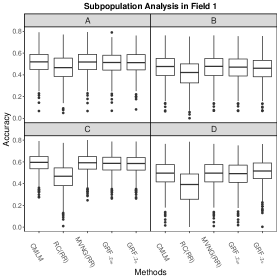
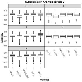
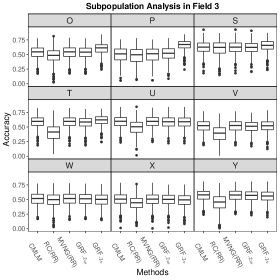
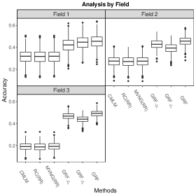
Figure 2: (1–3): Comparison of CMLM, RC(RR), MVNG(RR) and two proposed methods $\text{GRF}_{-Z_{bs}}$ and $\text{GRF}_{-Z_{b}}$ for each subpopulation (only $9$ of $14$ are shown in Field $3$ to improve clarity). (4): Comparison of CMLM, RC(RR), MVNG(RR) and three proposed methods $\text{GRF}_{-Z_{b}}$, $\text{GRF}_{-Z_{s}}$ and GRF for each field.

Table 1: Average accuracies and their standard deviations (in parentheses) for Data1 by five existing methods and three proposed methods ($\text{GRF}_{-Z_{b}}$, $\text{GRF}_{-Z_{s}}$ and GRF) for each field based on $1000$ independent random partitions of the data into training ($80\%$) and test ($20\%$) sets.

	Method
Field	RC		MVNG		$\widehat{\gamma}=\widehat{\sigma}_{s}^{2}/\widehat{\sigma}_{g}^{2}$
	RR	GAUSS	RR	GAUSS
1	0.3173 (0.0633)	0.3144 (0.0628)	0.3159 (0.0638)	0.3131 (0.0633)	0.0646
2	0.2727 (0.051)	0.2729 (0.0511)	0.2697 (0.0501)	0.2698 (0.0501)	0.3041
3	0.1913 (0.0362)	0.1904 (0.0363)	0.1883 (0.0361)	0.1873 (0.0363)	1.0087
	CMLM	$\text{GRF}_{-Z_{b}}$	$\text{GRF}_{-Z_{s}}$	GRF
1	0.3173 (0.0632)	0.4199 (0.0641)	0.4428 (0.064)	$\bm{0.4520}$ (0.0629)
2	0.2727 (0.0501)	0.4289 (0.0422)	0.3920 (0.0464)	$\bm{0.4558}$ (0.0410)
3	0.1930 (0.0361)	0.4672 (0.0301)	0.4395 (0.0305)	$\bm{0.4904}$ (0.0296)

The highest average accuracy across methods for each field is shown in bold.

4.3 Data2 Prediction

For the wheat dataset Data2, there is no subpopulation information. Thus, we do not need the component $\bm{Z}_{b}$ in the full GRF, and the corresponding subpopulation covariance structure $\bm{C}_{b}$ is ignorable. In the following, we report the performance of CMLM, IB, RC(RR, GAUSS), MVNG(RR, GAUSS), SpATS, $\text{GRF}_{-Z_{b}}$ and $\text{GRF}_{-Z_{bs}}$ based on $1000$ independent training–test partitions for the eight phenotypes in the wheat dataset Data2. Due to space limitation, the detailed results are relegated to Tables S5 and S6 of the supplementary material. In addition to the prediction results, the corresponding parameter estimates are reported in Table S7 in the supplementary material. For each partition, we split the dataset into training ($86\%$) and test ($14\%$) sets. To avoid overestimating the prediction accuracy for new genotypes, we split so that all observations for any genotype are contained entirely within the training set or entirely within the test set. In contrast, completely random partitioning often distributes observations for a given genotype to both training and test sets. Because test set predictions for such genotypes can directly utilize information about the genotype from the training set, measurements of prediction accuracy from completely random partitioning tend to be much higher than should be expected when predicting the performance of a new genotype whose phenotypic values are not part of the training data. For this reason, our results on prediction accuracy are not comparable to the results reported in Table 3 of Lado et al. (2013). However, we do include the methods considered by Lado et al. (2013) in our study, with some adjustments to improve methods when possible. In particular, Lado et al. (2013) presented results for an inferior-performing version of our IB approach that involved using genomic prediction techniques on the residuals from the fit of the IB model without genomic information. Results labeled IB in this paper refer to our implementation of the IB model described in Section 4. All the methods are implemented in R language. Our R code is included in the online supplementary material. They can also be found at
https://github.com/mxjki/Adjusting_for_Spatial_Effects_in_Genomic_Prediction.

Figure 3 shows the comparison of CMLM, IB, RC(RR), MVNG(RR), SpATS, $\text{GRF}_{-Z_{b}}$ and $\text{GRF}_{-Z_{bs}}$ in terms of accuracy. To allow for a clearer visual depiction of results, RC and MVNG results based on GAUSS kernels appear only in Tables S5 and S6 in the supplemental document. Table S5 shows that $\text{GRF}_{-Z_{b}}$ has the highest average accuracy among all methods for five of the eight environment $\times$ phenotype combinations and higher average accuracy than the most similar competing method (SpATS) for all eight environment $\times$ phenotype combinations when using the full set of SNPs. Spatial effects are strongest for the phenotype grain yield (GY) in Santa Rosa under two levels of water supply, mild water stress (MWS) and fully irrigated (FI), with estimated relative strength of spatial effects $\widehat{\gamma}$ is $2.4231$ and $4.5171$, respectively (see Table S7). Figures in Rodriguez-Alvarez et al. (2018) and Selle et al. (2019) provide a detailed description of the strong spatial effects. When spatial effects are strongest, Figure  3 shows that SpATs and $\text{GRF}_{-Z_{b}}$ clearly outperform other approaches, regardless of whether full or selected SNPs are used. When spatial effects are strong, the accuracy difference between $\text{GRF}_{-Z_{b}}$ and $\text{GRF}_{-Z_{bs}}$ is much larger than for other phenotypes. Figure 3 (and also Tables S5, S6 and S7) indicates that although the general results are not strongly sensitive to selection of SNPs prior to model fitting and analysis, the average accuracy of $\text{GRF}_{-Z_{b}}$ tends to decrease following SNP selection.

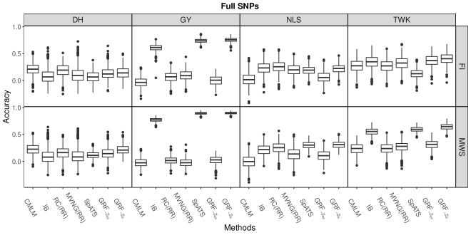
Figure 3: Comparisons of CMLM, IB, RC(RR), MVNG(RR), SpATS and two proposed methods $\text{GRF}_{-Z_{bs}}$ and $\text{GRF}_{-Z_{b}}$ with full and selected SNPs.

5 Simulation Study

This section reports results from simulation experiments designed to evaluate numerical performance of genomic predictions after adjusting for spatial effects.

5.1 Data1 Ranking

From the maize dataset Data1, we fit the full GRF model to obtain parameter estimates $\widehat{\mu},\widehat{\sigma}_{g},\widehat{\tau},\widehat{\sigma}_{b},\widehat{\sigma}_{s}$, and $\widehat{\sigma}_{\epsilon}$. These estimates provide $\widehat{\bm{C}}_{g}$ and $\widehat{\bm{\Sigma}}$, which determine the estimated mean and variance of the conditional multivariate normal distribution for $\bm{Z}_{g}$, $\bm{Z}_{b}$ and $\bm{Z}_{s}$ according to equations (2) and (3). Given these estimated parameters, let $\widetilde{\bm{Z}}_{g}$, $\widetilde{\bm{Z}}_{b}$ and $\widetilde{\bm{Z}}_{s}$ be generated simultaneously from a multivariate normal distribution where the mean and variance are specified in (2) and (3). And let $\tilde{\bm{e}}$ be generated from $\mathcal{N}(\bm{0},\widehat{\sigma}_{\epsilon}^{2}\bm{I})$. To allow different strengths of spatial effects, we simulate the response vector $\tilde{\bm{y}}=\widehat{\mu}\bm{1}+\widetilde{\bm{Z}}_{g}+\widetilde{\bm{Z}}_{b}+c\widetilde{\bm{Z}}_{s}+\tilde{\bm{e}}$, where $c\in\{1,2,3,4\}$ controls the strength of spatial effects. Given a simulated dataset, we fit the full GRF, $\text{GRF}_{-Z_{s}}$ and $\text{GRF}_{-Z_{b}}$ to predict $\tilde{\bm{y}}$. We repeat this simulation and fitting process $1000$ times.

In addition to prediction accuracy, we also compare the ability to rank plant genotypes. We compare the true rank-order $\bm{r}^{(o)}$ of the elements of $\widehat{\mu}\bm{1}+\widetilde{\bm{Z}}_{g}+\widetilde{\bm{Z}}_{b}$, with the rank-orders $\bm{r}^{(\text{GRF})}$, $\bm{r}^{(\text{GRF}_{-Z_{s}})}$ and $\bm{r}^{(\text{GRF}_{-Z_{b}})}$ of the predictions by computing the Spearman’s rank-order correlations $\rho_{s}(\bm{r}^{(o)},\bm{r}^{(\text{GRF})})$, $\rho_{s}(\bm{r}^{(o)},\bm{r}^{(\text{GRF}_{-Z_{s}})})$, and $\rho_{s}(\bm{r}^{(o)},\bm{r}^{(\text{GRF}_{-Z_{b}})})$ for each simulation replication.

Table 2 reports both the prediction accuracies and Spearman’s rank-order correlations. These two measurements are highly correlated. The full GRF is much better than $\text{GRF}_{-Z_{s}}$ and $\text{GRF}_{-Z_{b}}$ in terms of prediction accuracies and the similarities of rank-orders with the true rank-order $\bm{r}^{(o)}$. Because spatial effects and subpopulation effects for Data1 in each field are strong enough ($\widehat{\gamma}=0.0646$, $\widehat{\sigma}_{b}=0.3581$; $\widehat{\gamma}=0.3041$, $\widehat{\sigma}_{b}=0.3526$ and $\widehat{\gamma}=1.0087$, $\widehat{\sigma}_{b}=0.3939,$ respectively, for the three fields.) With spatial strength held constant, prediction performance in Table 2 improves across fields in accordance with the number of observations per field, likely due to the improvement of estimation with more data.

Table 2: Average prediction accuracies and Spearman’s rank-order correlations ($\rho_{s}$) based on 1000 simulations for Data1 by the full GRF, $\text{GRF}_{-Z_{s}}$ and $\text{GRF}_{-Z_{b}}$ for different spatial strengths.

Field	Strength	Accuracies			$\rho_{s}$
		GRF	$\text{GRF}_{-Z_{s}}$	$\text{GRF}_{-Z_{b}}$	GRF	$\text{GRF}_{-Z_{s}}$	$\text{GRF}_{-Z_{b}}$
1	1	$\bm{0.8249}$	0.8200	0.5041	$\bm{0.8076}$	0.8036	0.4711
	2	$\bm{0.8069}$	0.7853	0.4795	$\bm{0.7887}$	0.7676	0.4459
	3	$\bm{0.7860}$	0.7343	0.4672	$\bm{0.7659}$	0.7169	0.4332
	4	$\bm{0.7632}$	0.6738	0.4571	$\bm{0.7421}$	0.6595	0.4229
2	1	$\bm{0.8395}$	0.8317	0.5221	$\bm{0.8276}$	0.8196	0.5008
	2	$\bm{0.8129}$	0.7706	0.5070	$\bm{0.7995}$	0.7563	0.4858
	3	$\bm{0.7847}$	0.6900	0.4952	$\bm{0.7699}$	0.6762	0.4740
	4	$\bm{0.7554}$	0.6067	0.4836	$\bm{0.7395}$	0.5956	0.4627
3	1	$\bm{0.9135}$	0.9085	0.2835	$\bm{0.8986}$	0.8934	0.2760
	2	$\bm{0.8818}$	0.8505	0.2693	$\bm{0.8637}$	0.8310	0.2621
	3	$\bm{0.8486}$	0.7738	0.2601	$\bm{0.8286}$	0.7512	0.2531
	4	$\bm{0.8164}$	0.6940	0.2523	$\bm{0.7952}$	0.6693	0.2453

The highest average accuracy and highest average rank-order correlation across methods for each combination of field and spatial strength are shown in bold.

For each simulated data set, we predict the top $l$ inbred lines are by ranking our predictions of $\mathbb{Z}_{g}+\mathbb{Z}_{b}$, for $l\in\{1,\ldots,n\}$. We use $T_{l}$ as notation for the predicted group of top $l$ lines. Note that, due to estimation and prediction errors, the true rank-orders $\bm{r}^{o}_{l}$ of the lines in $T_{l}$ may not be $1,\ldots,l$. We evaluate the accuracy by the average median of $\bm{r}^{o}_{l}$ over 1000 simulations. The smaller the average median is, the better the predicted group is. In the following, we study the accuracy of the first ten groups, $T_{1},\ldots,T_{10}$, for different methods.

Figure 4 shows the average median of $\bm{r}^{(o)}_{l}$ for $l=1,\ldots,10$ for the full GRF, $\text{GRF}_{-Z_{s}}$ and $\text{GRF}_{-Z_{b}}$ on each field. The horizontal axis represents different groups while the vertical axis represents the corresponding average median of $\bm{r}^{(o)}_{I}$. We can see in Figure 4 that the full GRF performs consistently better than $\text{GRF}_{-Z_{s}}$ and $\text{GRF}_{-Z_{b}}$ which suggests that accounting for either spatial or subpopulation effects improves selection of the best plant genotypes.

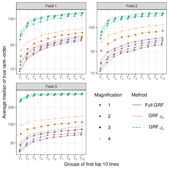
Figure 4: Rank-order analysis for Data1 using three different methods under different magnification ($c$) of the spatial effects. The Y-axis is on a logarithmic scale.

5.2 Data2 Ranking

For the wheat dataset Data2, we report the performances of $\text{GRF}_{-Z_{b}}$, $\text{GRF}_{-Z_{bs}}$ and CMLM based on $1000$ simulations, for each of the eight phenotypes. We achieve similar conclusions as in Data1. Due to space limitation, the details are relegated to Section S5 of the supplementary material.

6 Discussion

This paper investigates the problem of adjusting for spatial effects in genomic prediction. Our analysis of the maize dataset Data1 and the wheat dataset Data2 reveals the existence of spatial effects and heterogeneity across different subpopulation families. The spatial effects and heterogeneity, without proper treatment, can reduce the quality of phenotypic prediction and genotypic ranking. Under the Gaussian random field model, we propose an additive covariance matrix structure that incorporates genotype effects, spatial effects and subpopulation effects. We have also shown that by adjusting for spatial effects, we can improve the selection of top-performing plant genotypes.

As a guest Editor suggests, block cross-validation (Roberts et al., 2017) could be a more practical cross-validation method when the data are spatially correlated because it produces cross-validation errors that better match the magnitude of errors expected in practice. However, its effect on the ranking of the models has not been well understood other than few recondite applications where the spatial domains are disconnected (Hao et al., 2020). More exploration on this direction would be beneficial.

7 Acknowledgment

The authors thank the Joint Editor and the two reviewers whose constructive comments and suggestions led to a considerably improved version of the manuscript. The authors acknowledge the Iowa State University Plant Sciences Institute Scholars Program for financial support and the lab of Patrick S. Schnable and former graduate research assistant Sarah Hill–Skinner for collecting and sharing the maize data. This article is a product of the Iowa Agriculture and Home Economics Experiment Station, Ames, Iowa. Project No. IOW03617 is supported by USDA/NIFA and State of Iowa funds. Xiaojun Mao’s research is partially supported by Shanghai Sailing Program 19YF1402800. Any opinions, findings, conclusions or recommendations expressed in this publication are those of the authors and do not necessarily reflect the views of the U.S. Department of Agriculture or the Science and Technology Commission of Shanghai Municipality.

Supplement to “Adjusting for Spatial Effects in Genomic Prediction”
Xiaojun Mao, Somak Dutta, Raymond K. W. Wong and Dan Nettleton

Abstract

This document provides supplementary material to the article “Adjusting for Spatial Effects in Genomic Prediction” written by the same authors.

S1 Data pre-processing

In this section, we provide a detailed description of the pre-processing procedures for the maize dataset Data1 and the wheat dataset Data2.

Figure S1 shows the boxplot of the carbon dioxide emissions of the 25 subpopulations.

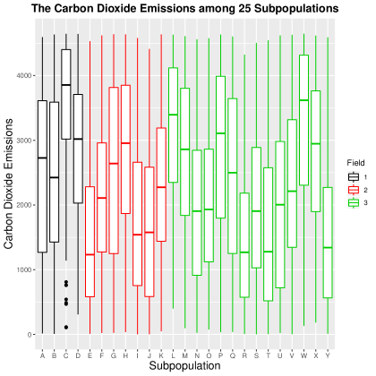
Figure S1: Carbon Dioxide Emissions among 25 subpopulations A through Y.

For the maize dataset Data1, Table S1 shows the average missing rate and average minor allele frequency (MAF) for SNP genotypes by chromosome after missing genotypes were imputed with LD-kNNi (Money et al., 2015).

Table S1: The average missing rate and average MAF after imputation for each chromosome.

Chromosome	1	2	3	4	5	6	7	8	9	10
Missing	0.1664	0.1607	0.1598	0.1657	0.1640	0.1592	0.1592	0.1642	0.1660	0.1592
MAF	0.1186	0.1101	0.1074	0.1129	0.1177	0.1091	0.1118	0.1108	0.1153	0.1113

After all missing SNP genotypes were imputed, we subdivided the 4660 observations into subsets corresponding to the three fields and, further, into subsets corresponding to the 25 subpopulations.

In each of these datasets, many SNP markers are identical to other SNP markers for all observations. We kept only one representative SNP marker in such cases and removed redundant SNPs. However, a huge number of SNP markers still remain. It is not only a computational burden for the marker kernel $\bm{C}_{g}$, but it also incorporates redundant information from highly correlated SNPs and useless information from SNPs unassociated with trait values. To get a more useful marker kernel, we used the R package $\mathrm{FarmCPU}$ (Liu et al., 2016) with default settings to select subsets of SNPs for computation of our marker kernel. This selection of SNPs was done separately for each subpopulation and each field for data1, and separately for each trait for data2. Table S2 shows the total number of SNP markers before and after removing the duplicated markers, the number of selected SNP markers for Data1 on Field 1, and the minimum MAF among the selected markers.

Table S2: The total number of SNP markers before and after removing the duplicated markers, the number of selected SNP markers for Data1 on Field 1, and the minimum MAF among the selected SNPs.

Chromosome	1	2	3	4	5	6	7	8	9	10
total	104827	81315	78369	73466	67423	58365	59577	59820	54013	50694
unique	95065	71524	68790	64492	60645	51272	51803	52687	47238	44470
selected	470	2666	789	300	503	290	580	343	124	401
min MAF	0.0171	0.0237	0.0171	0.0197	0.0184	0.0276	0.0184	0.0237	0.0145	0.0184

Table S2 shows that, after selection, the number of SNP markers is greatly reduced.

S2 Sensitivity to the parameter $\beta_{00}$

Table S3: The mean of accuracies for eight phenotypes by method $\text{GRF}_{-Z_{b}}$ ($\lambda_{00}=0.001$ and $\lambda_{00}=0.0001$) with full and selected SNPs based on $1000$ independent random partitions of the data into training ($86\%$) and test ($14\%$) sets.

		Full		Selected
Water Supply	Phenotype	$\text{GRF}_{-Z_{b}}$		$\text{GRF}_{-Z_{b}}$
	$\lambda_{00}$	$0.001$	$0.0001$	$0.001$	$0.0001$
FI	DH	0.8667	0.8668	0.8160	0.8185
	GY	0.8299	0.8305	0.8309	0.8314
	NKS	0.7160	0.7133	0.7004	0.6976
	TKW	0.8294	0.8284	0.7972	0.7968
MWS	DH	0.8231	0.8249	0.7732	0.7729
	GY	0.9275	0.9268	0.9269	0.9257
	NKS	0.7248	0.7244	0.7143	0.7140
	TKW	0.8867	0.8863	0.8696	0.8700

S3 Data1 prediction results

Table S4: Average accuracies for Data1 by five existing methods and two proposed methods ($\text{GRF}_{-Z_{bs}}$ and $\text{GRF}_{-Z_{b}}$) for each subpopulation based on $1000$ independent random partitions of the data into training ($80\%$) and test ($20\%$) sets. The highest average accuracy across methods for each subpopulation is shown in bold.

		Method
Field	Subpopulation	CMLM	RC		MVNG		$\text{GRF}_{-Z_{bs}}$	$\text{GRF}_{-Z_{b}}$	$\widehat{\gamma}=\widehat{\sigma}_{s}^{2}/\widehat{\sigma}_{g}^{2}$
			RR	GAUSS	RR	GAUSS
1	A	$\bm{0.5101}$	0.4568	0.4196	0.5098	0.5014	0.5036	0.5070	0.0220
	B	0.4706	0.4077	0.3544	$\bm{0.4715}$	0.4610	0.4657	0.4530	9e-04
	C	$\bm{0.5875}$	0.4594	0.4388	0.5855	0.5805	0.5788	0.5772	0.0000
	D	0.4939	0.3139	0.0779	0.4933	0.4803	0.4886	$\bm{0.5113}$	0.0249
2	E	0.5300	0.2966	0.1407	0.5293	0.5295	$\bm{0.5377}$	0.5308	0.0228
	F	0.4939	0.4102	0.3782	0.4925	0.4847	0.4812	$\bm{0.5564}$	0.0994
	G	0.5314	0.4670	0.4424	0.5314	0.5278	0.5291	$\bm{0.5466}$	0.0412
	H	0.5250	0.4421	0.3324	0.5250	0.5281	0.5295	$\bm{0.5527}$	0.0704
	I	0.5694	0.4629	0.4235	0.5688	0.5689	0.5674	$\bm{0.6097}$	0.0576
	J	0.4947	0.4741	0.4588	$\bm{0.4950}$	0.4916	0.4901	0.4841	0.0285
	K	$\bm{0.6179}$	0.4399	0.3275	0.6166	0.6044	0.6088	0.6014	0.0014
3	L	0.5116	0.4354	0.2586	0.5104	0.5102	0.5102	$\bm{0.5455}$	0.0498
	M	$\bm{0.5036}$	0.4427	0.4329	0.5024	0.5014	0.5005	0.5028	0.0276
	N	0.5162	0.1193	0.0646	0.5148	0.5131	0.5084	$\bm{0.5166}$	0.0375
	O	0.5381	0.4741	0.2939	0.5373	0.5279	0.5338	$\bm{0.6024}$	0.0670
	P	0.4983	0.4857	0.4807	0.4966	0.5048	0.5153	$\bm{0.6598}$	0.3922
	Q	0.5562	0.4979	0.4632	0.5529	0.5508	0.5536	$\bm{0.5959}$	0.1044
	R	0.5563	0.4380	0.1916	0.5567	0.5563	0.5551	$\bm{0.5802}$	0.0650
	S	0.6193	0.6057	0.5845	0.6188	0.6166	0.6147	$\bm{0.6482}$	0.0502
	T	0.5892	0.4056	0.3383	0.5875	0.5837	0.5795	$\bm{0.6143}$	0.0242
	U	0.5886	0.4930	0.4807	$\bm{0.5894}$	0.5795	0.5818	0.5815	0.0000
	V	0.5160	0.3830	0.3097	$\bm{0.5166}$	0.5076	0.5054	0.5162	0.0202
	W	0.5110	0.4842	0.4325	$\bm{0.5116}$	0.5049	0.5068	0.4959	0.0038
	X	0.4990	0.4314	0.4078	$\bm{0.4991}$	0.4960	0.4947	0.4861	0.0120
	Y	$\bm{0.5680}$	0.4432	0.3613	0.5662	0.5571	0.5593	0.5547	0.0015

S4 Data2 prediction results

Table S5: Average accuracies for eight phenotypes by methods (CMLM, IB, RC(RR, GAUSS), MVNG(RR, GAUSS), SpATS, $\text{GRF}_{-Z_{bs}}$ and $\text{GRF}_{-Z_{b}}$) with full SNPs based on $1000$ independent random partitions of the data into training ($86\%$) and test ($14\%$) sets. The highest average accuracy across methods for each of the nine methods is printed in bold for each phenotype.

		Full
WS	Phenotype	CMLM	IB	RC		MVNG		SpATS	$\text{GRF}_{-Z_{bs}}$	$\text{GRF}_{-Z_{b}}$
				RR	GAUSS	RR	GAUSS
FI	DH	$\bm{0.2091}$	0.0851	0.1863	0.1756	0.1084	0.1386	0.0672	0.1350	0.1435
	GY	-0.0346	0.6132	0.0662	0.0739	0.0934	-0.0022	0.7410	0.0015	$\bm{0.7575}$
	NKS	0.0181	0.2355	0.2539	$\bm{0.2776}$	0.1979	0.0999	0.1898	0.0638	0.2214
	TKW	0.2720	0.3442	0.2682	0.2722	0.3217	0.3509	0.1252	0.3692	$\bm{0.4040}$
MWS	DH	$\bm{0.2218}$	0.0945	0.1587	0.1571	0.1017	0.1458	0.1157	0.1516	0.2174
	GY	-0.0264	0.7734	0.0146	0.0135	-0.0273	-0.0110	0.8946	0.0183	$\bm{0.8988}$
	NKS	-0.0033	0.2149	0.2487	0.2576	0.1328	0.1005	0.3015	0.1095	$\bm{0.3112}$
	TKW	0.2354	0.5530	0.2350	0.2394	0.2710	0.2869	0.5938	0.3132	$\bm{0.6443}$

Table S6: Average accuracies for eight phenotypes by methods (CMLM, IB, RC(RR, GAUSS), MVNG(RR, GAUSS), SpATS, $\text{GRF}_{-Z_{bs}}$ and $\text{GRF}_{-Z_{b}}$) with selected SNPs based on $1000$ independent random partitions of the data into training ($86\%$) and test ($14\%$) sets. The highest average accuracy across methods for each of the nine methods is printed in bold for each phenotype.

		Selected
WS	Phenotype	CMLM	IB	RC		MVNG		SpATS	$\text{GRF}_{-Z_{bs}}$	$\text{GRF}_{-Z_{b}}$
				RR	GAUSS	RR	GAUSS
FI	DH	0.1637	0.0772	0.1540	0.1867	$\bm{0.1928}$	0.1341	0.0672	-0.0906	-0.0234
	GY	-0.0396	0.6184	0.1395	0.1350	0.1505	-0.0112	0.7410	-0.1080	$\bm{0.7618}$
	NKS	0.0961	0.2070	0.1922	$\bm{0.2588}$	0.1510	0.0958	0.1898	-0.0095	0.1881
	TKW	0.1997	0.2030	0.1096	0.2542	0.2666	$\bm{0.2999}$	0.1252	0.0008	0.1442
MWS	DH	0.1443	0.0317	0.0891	$\bm{0.1521}$	0.0604	0.1406	0.1157	-0.0198	0.1236
	GY	-0.0324	0.7751	0.1068	0.1048	0.0338	-0.0109	0.8946	-0.0843	$\bm{0.8979}$
	NKS	-0.0322	0.2342	0.2433	0.2626	0.1073	0.1219	$\bm{0.3015}$	0.0031	0.2925
	TKW	0.2546	0.5276	0.2275	0.2242	0.2471	0.2635	$\bm{0.5938}$	-0.0002	0.5870

Table S7: The spatial parameter estimates for eight phenotypes by method $\text{GRF}_{-Z_{b}}$ with full and selected SNPs.

		Full			Selected
Water Supply	Phenotype	$\beta_{01}$	$\beta_{10}$	$\widehat{\gamma}$	$\beta_{01}$	$\beta_{10}$	$\widehat{\gamma}$
FI	DH	0.0344	0.4656	0.0277	0.0142	0.4858	0.0165
	GY	0.0587	0.4413	2.4231	0.0612	0.4388	2.6715
	NKS	0.0077	0.4923	0.1670	0.0116	0.4884	0.1629
	TKW	0.0264	0.4736	0.0877	0.0270	0.4730	0.0724
MWS	DH	0.0394	0.4606	0.0451	0.0333	0.4667	0.0597
	GY	0.0644	0.4356	4.5171	0.0688	0.4312	4.7537
	NKS	0.0596	0.4404	0.2502	0.0569	0.4431	0.2510
	TKW	0.0861	0.4139	0.4125	0.1109	0.3891	0.4787

S5 Data2 ranking

Table S8 reports both the prediction accuracies and Spearman’s rank-order correlations. As before, these two measurements are highly correlated. The results show that with strong spatial effects, i.e., phenotype GY under full irrigated (FI) conditions and mild water stress, $\text{GRF}_{-Z_{b}}$ is much better than $\text{GRF}_{-Z_{bs}}$ in terms of prediction accuracies and the similarities of rank-orders with the true rank-order $\bm{r}^{(o)}$. We can see in Figure S2 that $\text{GRF}_{-Z_{b}}$ is consistently better than $\text{GRF}_{-Z_{bs}}$. This provides the evidence that accounting for spatial effects improves selection of the best plant genotypes.

Table S8: Average prediction accuracies and Spearman’s rank-order correlations ($\rho_{s}$) based on 1000 simulations for different phenotypes by $\text{GRF}_{-Z_{bs}}$ and $\text{GRF}_{-Z_{b}}$ with full and selected SNPs under full irrigated (FI) conditions and mild water stress.

		Full				Selected
		Accuracies		$\rho_{s}$		Accuracies		$\rho_{s}$
WS	Phenotype	$\text{GRF}_{-Z_{bs}}$	$\text{GRF}_{-Z_{b}}$	$\text{GRF}_{-Z_{bs}}$	$\text{GRF}_{-Z_{b}}$	$\text{GRF}_{-Z_{bs}}$	$\text{GRF}_{-Z_{b}}$	$\text{GRF}_{-Z_{bs}}$	$\text{GRF}_{-Z_{b}}$
FI	DH	0.9870	0.9895	0.9851	0.9879	0.9604	0.9606	0.9558	0.9562
	GY	0.7241	0.8401	0.7056	0.8261	0.7123	0.8334	0.6940	0.8196
	NKS	0.9148	0.9302	0.9056	0.9222	0.9067	0.9184	0.8972	0.9098
	TKW	0.9622	0.9697	0.9574	0.9658	0.9505	0.9558	0.9446	0.9504
MWS	DH	0.9749	0.9783	0.9714	0.9751	0.9467	0.9503	0.9405	0.9443
	GY	0.6257	0.8201	0.6060	0.8052	0.6251	0.8195	0.6077	0.8051
	NKS	0.9036	0.9184	0.8938	0.9099	0.8927	0.9064	0.8818	0.8966
	TKW	0.9336	0.9702	0.9258	0.9660	0.9210	0.9533	0.9122	0.9478

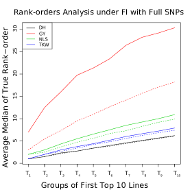
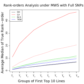
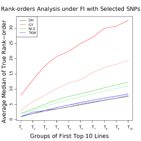
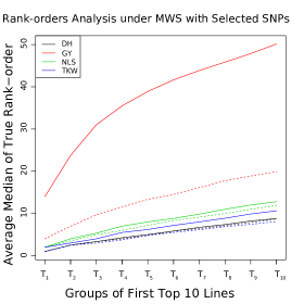
Figure S2: Comparisons of $\text{GRF}_{-Z_{bs}}$ and $\text{GRF}_{-Z_{b}}$ with full and selected SNPs under full irrigated (FI) conditions and mild water stress. The solid lines are for $\text{GRF}_{-Z_{bs}}$, while dashed lines are for $\text{GRF}_{-Z_{b}}$.

References

- (1)
- Bernal-Vasquez et al. (2014) Bernal-Vasquez, A.-M., Möhring, J., Schmidt, M., Schönleben, M., Schön, C.-C., and Piepho, H.-P. (2014), “The importance of phenotypic data analysis for genomic prediction-a case study comparing different spatial models in rye,” BMC Genomics, 15(1), 646.
- Besag et al. (1995) Besag, J., Green, P., Higdon, D., and Mengersen, K. (1995), “Bayesian computation and stochastic systems,” Statistical science, pp. 3–41.
- Besag and Green (1993) Besag, J., and Green, P. J. (1993), “Spatial Statistics and Bayesian Computation,” Journal of the Royal Statistical Society. Series B (Methodological), 55(1), 25–37.
- Besag and Higdon (1999) Besag, J., and Higdon, D. (1999), “Bayesian analysis of agricultural field experiments,” Journal of the Royal Statistical Society: Series B (Statistical Methodology), 61(4), 691–746.
- Besag and Kooperberg (1995) Besag, J., and Kooperberg, C. (1995), “On conditional and intrinsic autoregressions,” Biometrika, 82(4), 733–746.
- Cabrera-Bosquet et al. (2012) Cabrera-Bosquet, L., Crossa, J., von Zitzewitz, J., Serret, M. D., and Luis Araus, J. (2012), “High-throughput Phenotyping and Genomic Selection: The Frontiers of Crop Breeding ConvergeF,” Journal of Integrative Plant Biology, 54(5), 312–320.
- Crossa et al. (2006) Crossa, J., Burgueño, J., Cornelius, P. L., McLaren, G., Trethowan, R., and Krishnamachari, A. (2006), “Modeling genotype environment interaction using additive genetic covariances of relatives for predicting breeding values of wheat genotypes,” Crop Science, 46(4), 1722–1733.
- Cullis and Gleeson (1991) Cullis, B., and Gleeson, A. (1991), “Spatial analysis of field experiments-an extension to two dimensions,” Biometrics, pp. 1449–1460.
- Cullis et al. (1998) Cullis, B., Gogel, B., Verbyla, A., and Thompson, R. (1998), “Spatial analysis of multi-environment early generation variety trials,” Biometrics, pp. 1–18.
- Durban et al. (2003) Durban, M., Hackett, C. A., McNicol, J. W., Newton, A. C., Thomas, W. T., and Currie, I. D. (2003), “The practical use of semiparametric models in field trials,” Journal of agricultural, biological, and environmental statistics, 8(1), 48.
- Dutta and Mondal (2015) Dutta, S., and Mondal, D. (2015), “An h-likelihood method for spatial mixed linear models based on intrinsic auto-regressions,” Journal of the Royal Statistical Society: Series B (Statistical Methodology), 77(3), 699–726.
- Dutta and Mondal (2016) Dutta, S., and Mondal, D. (2016), “REML estimation with intrinsic Matérn dependence in the spatial linear mixed model,” Electronic Journal of Statistics, 10(2), 2856–2893.
- Endelman (2011) Endelman, J. B. (2011), “Ridge regression and other kernels for genomic selection with R package rrBLUP,” The Plant Genome, 4(3), 250–255.
- Gilmour et al. (1997) Gilmour, A. R., Cullis, B. R., and Verbyla, A. P. (1997), “Accounting for natural and extraneous variation in the analysis of field experiments,” Journal of Agricultural, Biological, and Environmental Statistics, pp. 269–293.
- Gleeson and Cullis (1987) Gleeson, A. C., and Cullis, B. R. (1987), “Residual maximum likelihood (REML) estimation of a neighbour model for field experiments,” Biometrics, pp. 277–287.
- Hao et al. (2020) Hao, T., Elith, J., Lahoz-Monfort, J. J., and Guillera-Arroita, G. (2020), “Testing whether ensemble modelling is advantageous for maximising predictive performance of species distribution models,” Ecography, . forthcoming.
- Lado et al. (2013) Lado, B., Matus, I., Rodríguez, A., Inostroza, L., Poland, J., Belzile, F., del Pozo, A., Quincke, M., Castro, M., and von Zitzewitz, J. (2013), “Increased genomic prediction accuracy in wheat breeding through spatial adjustment of field trial data,” G3: Genes— Genomes— Genetics, 3(12), 2105–2114.
- Lipka et al. (2012) Lipka, A. E., Tian, F., Wang, Q., Peiffer, J., Li, M., Bradbury, P. J., Gore, M. A., Buckler, E. S., and Zhang, Z. (2012), “GAPIT: genome association and prediction integrated tool,” Bioinformatics, 28(18), 2397–2399.
- Liu et al. (2016) Liu, X., Huang, M., Fan, B., Buckler, E. S., and Zhang, Z. (2016), “Iterative usage of fixed and random effect models for powerful and efficient genome-wide association studies,” PLoS Genet, 12(2), e1005767.
- Masuka et al. (2012) Masuka, B., Araus, J. L., Das, B., Sonder, K., and Cairns, J. E. (2012), “Phenotyping for abiotic stress tolerance in maizef,” Journal of Integrative Plant Biology, 54(4), 238–249.
- McCullagh and Clifford (2006) McCullagh, P., and Clifford, D. (2006), Evidence for conformal invariance of crop yields,, in Proceedings of the Royal Society of London A: Mathematical, Physical and Engineering Sciences, Vol. 462, The Royal Society, pp. 2119–2143.
- McVean (2009) McVean, G. (2009), “A genealogical interpretation of principal components analysis,” PLoS Genetics, 5(10), e1000686.
- Mondal et al. (2020) Mondal, S., Dutta, S., Crespo-Herrera, L., Huerta-Espino, J., Braun, H. J., and Singh, R. P. (2020), “Fifty years of semi-dwarf spring wheat breeding at CIMMYT: Grain yield progress in optimum, drought and heat stress environments,” Field Crops Research, 250, 107757.
- Money et al. (2015) Money, D., Gardner, K., Migicovsky, Z., Schwaninger, H., Zhong, G.-Y., and Myles, S. (2015), “LinkImpute: Fast and Accurate Genotype Imputation for Nonmodel Organisms,” G3: Genes— Genomes— Genetics, 5(11), 2383–2390.
- Morota and Gianola (2014) Morota, G., and Gianola, D. (2014), “Kernel-based whole-genome prediction of complex traits: a review,” Frontiers in Genetics, 5.
- Morota et al. (2013) Morota, G., Koyama, M., Rosa, G. J., Weigel, K. A., and Gianola, D. (2013), “Predicting complex traits using a diffusion kernel on genetic markers with an application to dairy cattle and wheat data,” Genet Sel Evol, 45, 17.
- Ober et al. (2011) Ober, U., Erbe, M., Long, N., Porcu, E., Schlather, M., and Simianer, H. (2011), “Predicting genetic values: a kernel-based best linear unbiased prediction with genomic data,” Genetics, 188(3), 695–708.
- Price et al. (2006) Price, A. L., Patterson, N. J., Plenge, R. M., Weinblatt, M. E., Shadick, N. A., and Reich, D. (2006), “Principal components analysis corrects for stratification in genome-wide association studies,” Nature Genetics, 38(8), 904.
- Pritchard et al. (2000) Pritchard, J. K., Stephens, M., Rosenberg, N. A., and Donnelly, P. (2000), “Association mapping in structured populations,” The American Journal of Human Genetics, 67(1), 170–181.
- Reich et al. (2008) Reich, D., Price, A. L., and Patterson, N. (2008), “Principal component analysis of genetic data,” Nature Genetics, 40(5), 491–492.
- Roberts et al. (2017) Roberts, D. R., Bahn, V., Ciuti, S., Boyce, M. S., Elith, J., Guillera-Arroita, G., Hauenstein, S., Lahoz-Monfort, J. J., Schröder, B., Thuiller, W. et al. (2017), “Cross-validation strategies for data with temporal, spatial, hierarchical, or phylogenetic structure,” Ecography, 40(8), 913–929.
- Rodriguez-Alvarez et al. (2018) Rodriguez-Alvarez, M. X., Boer, M. P., van Eeuwijk, F. A., and Eilers, P. H. (2018), “Correcting for spatial heterogeneity in plant breeding experiments with P-splines,” Spatial Statistics, 23, 52–71.
- Selle et al. (2019) Selle, M. L., Steinsland, I., Hickey, J. M., and Gorjanc, G. (2019), “Flexible modelling of spatial variation in agricultural field trials with the R package INLA,” Theoretical and Applied Genetics, 132(12), 3277–3293.
- Stroup (2002) Stroup, W. W. (2002), “Power analysis based on spatial effects mixed models: A tool for comparing design and analysis strategies in the presence of spatial variability,” Journal of Agricultural, Biological, and Environmental Statistics, 7(4), 491–511.
- Stroup et al. (1994) Stroup, W. W., Baenziger, P. S., and Mulitze, D. K. (1994), “Removing spatial variation from wheat yield trials: a comparison of methods,” Crop Science, 34(1), 62–66.
- Stroup and Mulitze (1991) Stroup, W. W., and Mulitze, D. (1991), “Nearest neighbor adjusted best linear unbiased prediction,” The American Statistician, 45(3), 194–200.
- VanRaden (2008) VanRaden, P. (2008), “Efficient methods to compute genomic predictions,” Journal of Dairy Science, 91(11), 4414–4423.
- Verbyla et al. (1999) Verbyla, A. P., Cullis, B. R., Kenward, M. G., and Welham, S. J. (1999), “The analysis of designed experiments and longitudinal data by using smoothing splines,” Journal of the Royal Statistical Society: Series C (Applied Statistics), 48(3), 269–311.
- White et al. (2012) White, J. W., Andrade-Sanchez, P., Gore, M. A., Bronson, K. F., Coffelt, T. A., Conley, M. M., Feldmann, K. A., French, A. N., Heun, J. T., Hunsaker, D. J. et al. (2012), “Field-based phenomics for plant genetics research,” Field Crops Research, 133, 101–112.
- Yu et al. (2008) Yu, J., Holland, J. B., McMullen, M. D., and Buckler, E. S. (2008), “Genetic design and statistical power of nested association mapping in maize,” Genetics, 178(1), 539–551.
- Yu et al. (2006) Yu, J., Pressoir, G., Briggs, W. H., Bi, I. V., Yamasaki, M., Doebley, J. F., McMullen, M. D., Gaut, B. S., Nielsen, D. M., Holland, J. B. et al. (2006), “A unified mixed-model method for association mapping that accounts for multiple levels of relatedness,” Nature Genetics, 38(2), 203–208.
- Zhang et al. (2010) Zhang, Z., Ersoz, E., Lai, C.-Q., Todhunter, R. J., Tiwari, H. K., Gore, M. A., Bradbury, P. J., Yu, J., Arnett, D. K., Ordovas, J. M. et al. (2010), “Mixed linear model approach adapted for genome-wide association studies,” Nature Genetics, 42(4), 355–360.
- Zimmerman and Harville (1991) Zimmerman, D. L., and Harville, D. A. (1991), “A random field approach to the analysis of field-plot experiments and other spatial experiments,” Biometrics, pp. 223–239.