Boosting the performance of the Quantum Otto heat engines

Abstract

To optimize the performance of a heat engine in finite-time cycle, it is important to understand the finite-time effect of thermodynamic processes. Previously, we have shown that extra work is needed to complete a quantum adiabatic process in finite time, and proved that the extra work follows a $\mathcal{C}/\tau^{2}$ scaling for long control time $\tau$. There the oscillating part of the extra work is neglected due to the complex energy-level structure of the particular quantum system. However, such oscillation of the extra work can not be neglected in some quantum systems with simple energy-level structure, e. g. the two-level system or the quantum harmonic oscillator. In this paper, we build the finite-time quantum Otto engine on these simple systems, and find that the oscillating extra work leads to a jagged edge in the constraint relation between the output power and the efficiency. By optimizing the control time of the quantum adiabatic processes, the oscillation in the extra work is utilized to enhance the maximum power and the efficiency. We further design special control schemes with the zero extra work at the specific control time. Compared to the linear control scheme, these special control schemes of the finite-time adiabatic process improve the maximum power and the efficiency of the finite-time Otto engine.

I Introduction

Quantum thermodynamics (Maruyama et al., 2009; Esposito et al., 2009; Campisi et al., 2011; Strasberg et al., 2017; Vinjanampathy and Anders, 2016) studies the effect of quantum characteristics, e. g. coherence (Scully et al., 2003; Quan et al., 2006; Solinas and Gasparinetti, 2016; Francica et al., 2019), entanglement (Benatti et al., 2003; Kraus et al., 2008; Altintas et al., 2014; Tavakoli et al., ), and quantum many-body effect (Jaramillo et al., 2016; Ma et al., 2017; Bengtsson et al., 2018; Chen et al., 2018) on the thermodynamic property of the system. One important topic is to find quantum heat engines as counterparts of the classical ones. To design a practical heat engine with non-zero output power, the finite-time quantum thermodynamics (Curzon and Ahlborn, 1975; Salamon and Berry, 1983; Esposito et al., 2010; Andresen, 2011; Whitney, 2014; Dann et al., 2019) needs to be studied instead of quasi-static thermodynamics (Quan et al., 2007; Ma et al., 2017; Bengtsson et al., 2018; Chen et al., 2018). Therefore understanding the finite-time effect of thermodynamic processes is crucial to the optimization of the finite-time heat engine (Tu, 2008; Rutten et al., 2009; Whitney, 2014; Alecce et al., 2015; Shiraishi et al., 2016; Deffner, 2018). Based on the universal $\mathcal{C}/\tau$ scaling of the entropy production in finite-time isothermal processes (Salamon and Berry, 1983), the efficiency at the maximum power is obtained analytically for the finite-time Carnot-like engine (Curzon and Ahlborn, 1975; Schmiedl and Seifert, 2007; Esposito et al., 2010; Cavina et al., 2017). The trade-off relation between efficiency and power is further established recently (Shiraishi et al., 2016; Ryabov and Holubec, 2016; Long and Liu, 2016; Holubec and Ryabov, 2016; Ma et al., 2018a, b) for finite-time Carnot cycle. The finite-time heat engine of other types, e. g. the finite-time Otto engine, has been studied (Abah et al., 2012; Roßnagel et al., 2014; Alecce et al., 2015; Karimi and Pekola, 2016; Insinga et al., 2016; Campisi and Fazio, 2016; Kosloff and Rezek, 2017; Deffner, 2018; Erdman et al., 2018; Denzler and Lutz, ) and is shown with better performance by the technique of the shortcut to adiabatic (Chen et al., 2010; Deng et al., 2013; Abah and Lutz, 2018; Deng et al., 2018; Çakmak and Özgür E. Müstecaplıoğlu, 2019). Yet, the optimization of the finite-time Otto engine lacks a general principle compared to the universal $\mathcal{C}/\tau$ scaling of the entropy production in the finite-time Carnot-like engine.

Evaluating the finite-time effect of the adiabatic processes is the key to the optimization of the finite-time Otto engine, which consists two adiabatic processes and two isochoric processes. We consider the situation where the time consuming of the finite-time isochoric processes can be neglected compared to the finite-time adiabatic processes (Chotorlishvili et al., 2016; Abah and Lutz, 2018). During the finite-time adiabatic process, the system is isolated from the environment and evolves under the time-dependent Hamiltonian (Su et al., 2018). When energy levels of different states do not cross, the quantum adiabatic approximation is valid for long control time (Quan et al., 2007). In this situation, the theorem of high-order adiabatic approximation provides a perturbative technique to derive the finite-time correction to higher orders of the inverse control time (Sun, 1988; Wilczek and Shapere, 1989; Sun, 1990; Rigolin et al., 2008). It requires positive extra work to complete the adiabatic process in finite time.

In our previous paper (Chen et al., ), we find that the extra work in the finite-time adiabatic process can be naturally divided into the mean extra work and the oscillating extra work. With the increasing control time $\tau$, the mean extra work decreases monotonously, obeying a general $\mathcal{C}/\tau^{2}$ scaling behavior. The oscillating extra work oscillates around zero for larger $\tau$, and is neglected due to the incommensurable energy of different states in large systems. Yet, this oscillating extra work can not be neglected for the system with simple energy-level structure. In this paper, we continue the study of the oscillating extra work, and show its effects on some simple systems, such as the two-level system and the quantum harmonic oscillator. We find that the oscillation of the extra work can be utilized to enhance the output power of the heat engine. Besides, we obtain special control schemes of the adiabatic processes with zero extra work at the specific control time. The special control scheme further improves the maximum power of the Otto engine.

This paper is organized as follows. In Sec. II, we review the generic finite-time quantum Otto engine, and list the dependence of the power and the efficiency on the extra work in the finite-time adiabatic processes for later discussion. In Sec. III and IV, the finite-time quantum Otto cycles on two-level system and quantum harmonic oscillator are studied, respectively. The conclusion is given in Sec. V.

II Finite-time Quantum Otto engine

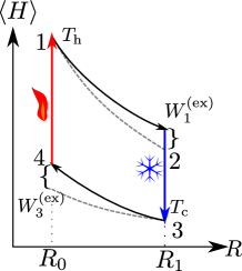
Figure 1: Energy-parameter ($\left\langle H\right\rangle-R$) diagram of the finite-time Otto cycle. The solid line with arrows presents the finite-time cycle, where two vertical colored lines present the isochoric processes (red for heating and blue for cooling), and two black lines present the finite-time adiabatic processes. The dashed lines present the quasi-static adiabatic processes. The extra work in the two finite-time adiabatic processes is marked as $W_{1}^{(\mathrm{ex})}(\tau_{1})$ and $W_{3}^{(\mathrm{ex})}(\tau_{3})$ .

In this section, we briefly review the finite-time Otto cycle. A generic finite-time Otto cycle consists four strokes, two finite-time adiabatic processes and two finite-time isochoric processes, illustrated on $\left\langle H\right\rangle-R$ diagram in Fig. 1.

In the finite-time adiabatic processes ($1\rightarrow 2$ and $3\rightarrow 4$) with the control time $\tau_{1}$ and $\tau_{3}$, the work is performed by tuning the parameter $R(t)$ in the Hamiltonian $H(t)\equiv H[R(t)]$, from $R_{0}$ to $R_{1}$ in the process $1\rightarrow 2$ and inversely in $3\rightarrow 4$. The system evolves under the time-dependent Hamiltonian as $\dot{\rho}=-i[H(t),\rho]$. The work done for the finite-time adiabatic process equals to the change of the internal energy

$$W(\tau)=\mathrm{Tr}[\rho(\tau)H(\tau)]-\mathrm{Tr}[\rho(0)H(0)],$$ (1)

where $\tau$ is the control time of the adiabatic process. The initial state $\rho(0)$ is a thermal state, while the final state $\rho(\tau)$ is not necessarily a thermal state. The finite-time adiabatic process requires more work compared to the quasi-static one. In Ref. (Chen et al., ), we rewrite the work as

$$W(\tau)=W^{\mathrm{adi}}+W^{(\mathrm{ex})}(\tau),$$ (2)

where $W^{\mathrm{adi}}$ is the work done in the quasi-static adiabatic process with infinite control time, and $W^{(\mathrm{ex})}(\tau)$ is the extra work for the finite-time adiabatic process.

We have shown that the extra work can be naturally divided into the mean extra work and the oscillating extra work

$$W^{\mathrm{(ex)}}(\tau)=W^{\mathrm{(mean)}}(\tau)+W^{\mathrm{(osc)}}(\tau).$$ (3)

The mean extra work decreases monotonously for longer control time $\tau$, satisfying the $\mathcal{C}/\tau^{2}$ scaling behavior. The oscillating extra work oscillates around zero with the increasing control time. For a large and complicated physical system, the oscillating extra work is usually neglected due to the incommensurable energy levels of different states (Chen et al., ). However, in quantum systems with simple energy-level structure, the contribution of the oscillating extra work should be taken into account.

To evaluate the efficiency, one needs to obtain the heat transfer in the isochoric process $4\rightarrow 1$ ($2\rightarrow 3$). Since no work is performed in this process, the heat is determined by the change of the internal energy. In the process $4\rightarrow 1$, the system absorbs the heat from the hot source $Q_{\mathrm{h}}=\left\langle H\right\rangle_{1}-\left\langle H\right\rangle_{4}>0$, while the system releases the heat to the cold sink $Q_{\mathrm{c}}=\left\langle H\right\rangle_{3}-\left\langle H\right\rangle_{2}<0$ in the process $2\rightarrow 3$. The time consuming of the isochoric process can be neglected compared to that of the adiabatic process (Chotorlishvili et al., 2016; Abah and Lutz, 2018). For a whole cycle, the net work is $W_{\mathrm{T}}=Q_{\mathrm{h}}-\left|Q_{\mathrm{c}}\right|$ with the efficiency $\eta=W_{\mathrm{T}}/Q_{\mathrm{h}}$.

In Ref. (Chen et al., ), we have obtained the power

$$P=\frac{W_{\mathrm{T}}^{\mathrm{adi}}-W_{1}^{(\mathrm{ex})}(\tau_{1})-W_{3}^{(\mathrm{ex})}(\tau_{3})}{\tau_{1}+\tau_{3}},$$ (4)

and the efficiency

$$\eta=\frac{W_{\mathrm{T}}^{\mathrm{adi}}-W_{1}^{(\mathrm{ex})}(\tau_{1})-W_{3}^{(\mathrm{ex})}(\tau_{3})}{Q_{\mathrm{h}}^{\mathrm{adi}}-W_{3}^{(\mathrm{ex})}(\tau_{3})}$$ (5)

for the finite-time Otto cycle. Here, $W_{\mathrm{T}}^{\mathrm{adi}}$ and $Q_{\mathrm{h}}^{\mathrm{adi}}$ denote the net work and the heat absorbed from the hot source in the quasi-static Otto cycle. $W_{1}^{(\mathrm{ex})}(\tau_{1})$ and $W_{3}^{(\mathrm{ex})}(\tau_{3})$ denote the extra work for the finite-time adiabatic processes $1\rightarrow 2$ and $3\rightarrow 4$ respectively. For given control time $\tau_{1}$ and $\tau_{3}$, higher power and efficiency can be achieved by optimizing the protocol to reduce the extra work $W_{1}^{(\mathrm{ex})}(\tau_{1})$ and $W_{3}^{(\mathrm{ex})}(\tau_{3})$.

In the previous paper, the constraint relation between the efficiency and the output power is obtained by neglecting the oscillating extra work for the system with complex energy-level structure. We only consider the mean part in the extra work $W_{1}^{(\mathrm{ex})}(\tau_{1})\approx\Sigma_{1}/\tau_{1}^{2}$ and $W_{3}^{(\mathrm{ex})}(\tau_{3})\approx\Sigma_{3}/\tau_{3}^{2}$, and obtain the efficiency at the maximum power as

$$\eta_{\mathrm{EMP}}=\frac{2\eta^{\mathrm{adi}}}{3-\eta^{\mathrm{adi}}/[1+(\Sigma_{1}/\Sigma_{3})^{1/3}]},$$ (6)

where $\eta^{\mathrm{adi}}$ is the efficiency of the quasi-static Otto cycle. Yet, such simplification fails for a quantum system with simple energy-level structure. We will explore the effect of the oscillating extra work for the simple quantum system in the following section.

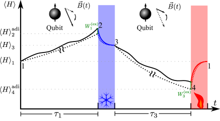
Figure 2: Finite-time Otto cycle of the two level system. The magnetic field $\vec{B}(t)$ is modulated in the finite-time adiabatic process. Similar to Fig. 1, the solid line presents the finite-time cycle, with the dashed line for the quasi-static one plotting for comparison. The time consuming for the two adiabatic processes is $\tau_{1}$ and $\tau_{3}$, while the time consuming for the isochoric processes is neglected.

III Two-level Otto engine

To show the effect of the oscillating extra work, we start with the simplest model of two-level system, a spin in a controllable magnetic field $\vec{B}(t)$. The Hamiltonian of the system reads

$$H=\mu\vec{B}(t)\cdot\vec{\sigma},$$ (7)

with the magnetic moment $\mu$ and the Pauli matrix $\vec{\sigma}$. We consider the magnetic field is modulated as $\vec{B}(t)=\left(B_{z}(t)+B_{\theta}\cos\theta\right)\vec{e}_{z}+B_{\theta}\sin\theta\vec{e}_{x}$ in the finite-time adiabatic process, where $\theta$ is the angle of the static magnetic field $B_{\theta}$. With the ratio of the magnetic field $\lambda=B_{z}(t)/B_{\theta}$, the Hamiltonian of the two-level system (Alecce et al., 2015) is rewritten as

$$H=\epsilon[(\lambda-\cos\theta)\sigma_{z}+\sin\theta\>\sigma_{x}],$$ (8)

by setting $\epsilon=\mu B_{\theta}$ as the unit of the energy. Here, $\lambda=\lambda(t)$ serves as the tuning parameter $R(t)$ in the finite-time adiabatic process. Figure 2 shows the finite-time Otto cycle realized on the two-level system. We present the finite-time cycle with the solid curve, and the quasi-static cycle with the dashed curve. In the two isochoric processes, the magnetic field is fixed and the system contacts with the hot source or the cold sink and reaches equilibrium (the red and blue curve).

To apply the high-order adiabatic approximation, we rewrite the Hamiltonian under the basis of instantaneous eigenstates (Sun, 1988) as

$$H=\epsilon\Lambda(t)\left(\left|e(t)\right\rangle\left\langle e(t)\right|-\left|g(t)\right\rangle\left\langle g(t)\right|\right),$$ (9)

where the instantaneous eigen-energy $\epsilon\Lambda(t)$ is determined by $\lambda(t)$ as

$$\Lambda(t)=\sqrt{\lambda^{2}-2\lambda\cos\theta+1}.$$ (10)

The instantaneous ground state is

$$\left|g(t)\right\rangle =1/N_{1}\left(\begin{array}[]{c}\lambda-\cos\theta-\Lambda\\ \sin\theta\end{array}\right),$$ (13)

and the instantaneous excited state is

$$\left|e(t)\right\rangle=1/N_{2}\left(\begin{array}[]{c}\lambda-\cos\theta+\Lambda\\ \sin\theta\end{array}\right),$$ (14)

where $N_{1}=[2\Lambda(\Lambda-\lambda+\cos\theta)]^{1/2}$ and $N_{2}=[2\Lambda(\Lambda+\lambda-\cos\theta)]^{1/2}$ are the normalized factors.

The initial state is a thermal state $\rho(0)=p_{g}\left|g(0)\right\rangle\left\langle g(0)\right|+p_{e}\left|e(0)\right\rangle\left\langle e(0)\right|$, where the distribution is $p_{g}=1-p_{e}=1/[1+\exp(-2\beta\epsilon\Lambda(0)]$ with the inverse temperature $\beta$. The density matrix at any time $t\in[0,\tau]$ is $\rho(t)=p_{g}\left|\psi_{g}(t)\right\rangle\left\langle\psi_{g}(t)\right|+p_{e}\left|\psi_{e}(t)\right\rangle\left\langle\psi_{e}(t)\right|$, where the state $\left|\psi_{n}(t)\right\rangle,\,n=e,g$ obeys the Schrodinger equation

$$i\partial_{t}\left|\psi_{n}(t)\right\rangle=H(t)\left|\psi_{n}(t)\right\rangle,$$ (15)

with the initial condition $\left|\psi_{n}(0)\right\rangle=\left|n(0)\right\rangle$. We express the state under the basis of the instantaneous eigenstates

$$\left|\psi_{n}(t)\right\rangle=c_{ng}(t)e^{i\phi(t)}\left|g(t)\right\rangle+c_{ne}(t)e^{-i\phi(t)}\left|e(t)\right\rangle$$ (16)

with the dynamical phase $\phi(t)=\epsilon\int_{0}^{t}\Lambda(t^{\prime})dt^{\prime}$. The Schrodinger equation by Eq. (15) gives the differential equations

$$\text{$\dot{c}$}_{ng} =e^{-2i\phi}\frac{\sin\left|\theta\right|\dot{\lambda}}{2\Lambda^{2}}c_{ne},$$ (17)

and

$$\dot{c}_{ne}=-e^{2i\phi}\frac{\sin\left|\theta\right|\dot{\lambda}}{2\Lambda^{2}}c_{ng}.$$ (18)

We consider a given protocol $\tilde{\lambda}(s)=\lambda(s\tau)$ with adjustable control time $\tau$, where $s=t/\tau\in[0,1]$ denotes the rescaled time parameter. The internal energy at the end of the adiabatic process is $\left\langle H(\tau)\right\rangle=(p_{e}-p_{g})[1-2\left|c_{eg}\left(\tau\right)\right|^{2}]\epsilon\tilde{\Lambda}(1)$ with the notation $\tilde{\Lambda}(s)=\Lambda(s\tau)$. Together with Eqs. (1) and (2), we obtain the quasi-static work

$$W^{\mathrm{adi}}=-\epsilon\tanh[\beta\epsilon\tilde{\Lambda}(0)][\tilde{\Lambda}(1)-\tilde{\Lambda}(0)],$$ (19)

and the extra work for the finite-time adiabatic process

$$W^{\mathrm{(ex)}}(\tau)=2\epsilon\tilde{\Lambda}(1)\tanh[\beta\epsilon\tilde{\Lambda}(0)]\left|c_{ge}\left(\tau\right)\right|^{2}.$$ (20)

At long control time limit, the first-order adiabatic approximation gives the asymptotic amplitude for Eq. (18)

$$c_{ge}^{[1]}\left(\tau\right) =\frac{i\sin\left|\theta\right|}{4\epsilon\tau}\left(\frac{\tilde{\lambda}^{\prime}(1)}{\tilde{\Lambda}(1)^{3}}e^{2i\tau\tilde{\phi}\left(1\right)}-\frac{\tilde{\lambda}^{\prime}(0)}{\tilde{\Lambda}(0)^{3}}\right),$$ (21)

where the dynamical phase is rewritten as $\tilde{\phi}(s)=\epsilon\int_{0}^{s}\tilde{\Lambda}(s^{\prime})ds^{\prime}$, and $\tilde{\lambda}^{\prime}(s)=\mathrm{d}\tilde{\lambda}(s)/\mathrm{d}s$ denotes the derivative of $\tilde{\lambda}(s)$. The derivation of Eq. (21) is attached in Appendix A. Substituting Eq. (21) into the extra work by Eq. (20), the asymptotic extra work is naturally divided into two parts according to Eq. (3), the mean extra work

$$W^{\mathrm{(mean)}}=\frac{\sin^{2}\theta\tilde{\Lambda}(1)}{8\epsilon\tau^{2}}\left(\frac{\tilde{\lambda^{\prime}}(1)^{2}}{\tilde{\Lambda}(1)^{6}}+\frac{\tilde{\lambda^{\prime}}(0)^{2}}{\tilde{\Lambda}(0)^{6}}\right)\tanh[\beta\epsilon\tilde{\Lambda}(0)],$$ (22)

and the oscillating extra work

$$W^{\mathrm{(osc)}}=-\frac{\sin^{2}\theta}{4\epsilon\tau^{2}}\frac{\tilde{\lambda^{\prime}}(1)\tilde{\lambda^{\prime}}(0)\cos[2\tau\tilde{\phi}(1)]}{\tilde{\Lambda}(1)^{2}\tilde{\Lambda}(0)^{3}}\tanh[\beta\epsilon\tilde{\Lambda}(0)].$$ (23)

To obtain the efficiency and the power for the finite-time Otto cycle, we need the net work $W_{\mathrm{T}}^{\mathrm{adi}}$ and the heat absorbed $Q_{\mathrm{h}}^{\mathrm{adi}}$ in the quasi-static Otto cycle with the infinite control time $\tau\rightarrow\infty$. The magnetic field $B_{z}(t)$ is modulated from $B_{0}$ to $B_{1}$ in the adiabatic process $1\rightarrow 2$, with the corresponding parameter $\lambda_{0}$ and $\lambda_{1}$ at the initial and final time. Since the population on the excited state remains unchanged during the quasi-static adiabatic processes (Quan et al., 2007), the internal energy of the four states follows immediately as $\left\langle H\right\rangle_{1}=-E_{0}\tanh(\beta_{\mathrm{h}}E_{0})$, $\left\langle H\right\rangle_{2}^{\mathrm{adi}}=-E_{1}\tanh(\beta_{\mathrm{h}}E_{0})$, $\left\langle H\right\rangle_{3}=-E_{1}\tanh(\beta_{\mathrm{c}}E_{1})$ and $\left\langle H\right\rangle_{4}^{\mathrm{adi}}=-E_{0}\tanh(\beta_{\mathrm{c}}E_{1})$. Here, $\beta_{l}=1/k_{\mathrm{B}}T_{l}$ is the inverse temperature for the hot source ($l=\mathrm{h}$) and the cold sink ($l=\mathrm{c}$), and $E_{j}=\epsilon\sqrt{\lambda_{j}^{2}-2\lambda_{j}\cos\theta+1},\,j=0,1$ gives the abbreviation of the eigen-energy. The net work of the quasi-static Otto cycle is

$$W_{\mathrm{T}}^{\mathrm{adi}} =(E_{0}-E_{1})[\tanh(\beta_{\mathrm{c}}E_{1})-\tanh(\beta_{\mathrm{h}}E_{0})]$$ (24)

The heat absorbed from the hot source is

$$Q_{\mathrm{h}}^{\mathrm{adi}}=E_{0}[\tanh(\beta_{\mathrm{c}}E_{1})-\tanh(\beta_{\mathrm{h}}E_{0})].$$ (25)

The efficiency of the quasi-static Otto cycle is $\eta^{\mathrm{adi}}=1-E_{1}/E_{0}$ (Quan et al., 2007). For the finite-time Otto cycle, the power and the efficiency are obtained by substituting the extra work by Eq. (20) and the quasi-static net work and heat by Eqs. (24) and (25) into Eqs. (4) and (5), respectively.

We compare the asymptotic extra work by Eqs (22) and (23) with the exact numerical result in Fig. 3(a). The exact numerical result is obtained by numerically solving Eq. (17) and (18). We choose the parameters $\theta=0.4,\,\epsilon=1,\,\lambda_{0}=0.1,\,\lambda_{1}=0.8$, and set temperatures for the hot source and cold sink as $k_{B}T_{\mathrm{h}}=5$ and $k_{B}T_{\mathrm{c}}=2$. We first adopt the linear protocol $\tilde{\lambda}_{l}(t/\tau_{1})=\tilde{\lambda}(0)+[\tilde{\lambda}(1)-\tilde{\lambda}(0)]t/\tau_{1}$. Figure 3(a) shows the extra work for the adiabatic process $1\rightarrow 2$ with different control time $\tau_{1}$, where the initial and the final tuning parameter are $\tilde{\lambda}(0)=\lambda_{0}$ and $\tilde{\lambda}(1)=\lambda_{1}$. The extra work (the blue curve) decreases with oscillation with the increasing control time, satisfying the $\mathcal{C}/\tau^{2}$ scaling (the red-dashed line). The asymptotic extra work from the first-order adiabatic approximation (the green-dashdotted curve) matches with the exact numerical result (the blue curve) at long control time.

We evaluate the performance of the finite-time Otto engine by modulating the control time $\tau_{1}$ and $\tau_{3}$ for the finite-time adiabatic processes. Figure 3(b) illustrates the constraint relation between efficiency and power. The red area presents the result with the mean extra work $W^{\mathrm{(mean)}}(\tau)$, where the oscillating extra work is neglected. The blue dots present the exact result by numerically calculating the extra work $W_{1}^{(\mathrm{ex})}(\tau_{1})$ and $W_{3}^{(\mathrm{ex})}(\tau_{3})$ in finite time. The oscillation of the extra work leads to a jagged edge in the constraint relation, and can be utilized to achieve larger maximum power.

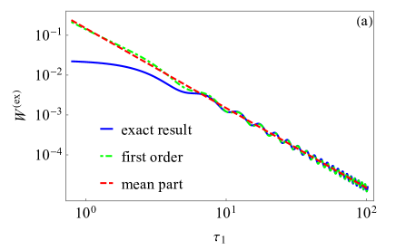
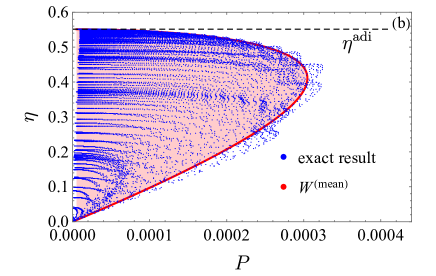
Figure 3: (a) The extra work for the adiabatic process $1\rightarrow 2$ with the linear protocol $\tilde{\lambda}_{l}$. The blue-solid curve, the green-dashdotted curve and the red-dashed line present the exact numerical result, the first-order adiabatic result, and the mean extra work, respectively, while the horizontal black-dashed line presents the quasi-static efficiency. The parameters are chosen as $\lambda_{0}=0.1$ and $\lambda_{1}=0.8$ with $\theta=0.4$ and $\epsilon=1$, with the temperatures $T_{\mathrm{h}}=5$ and $T_{\mathrm{c}}=2$. (b) the reachable power and efficiency for the finite-time two-level Otto engine. The red area only accounts for the mean extra work, while the blue dots present the exact numerical result.

To attain high power, we should reduce the extra work in the finite-time adiabatic processes at the given control time $\tau_{1}$ or $\tau_{3}$. The extra work by Eqs (22) and (23) approaches zero at the specific control time $\tau=n\pi/\tilde{\phi}(1),\,n=1,2,...$ with the condition $\tilde{\lambda^{\prime}}(1)/[\tilde{\Lambda}(1)]^{3}=\tilde{\lambda^{\prime}}(0)/[\tilde{\Lambda}(0)]^{3}$. We design such special protocol $\tilde{\lambda}_{s}(s)$ to satisfy this condition, determined by the implicit equation

$$s=\frac{\frac{\tilde{\lambda}(s)-\cos\theta}{\tilde{\Lambda}(s)}-\frac{\tilde{\lambda}(0)-\cos\theta}{\tilde{\Lambda}(0)}}{\frac{\tilde{\lambda}(1)-\cos\theta}{\tilde{\Lambda}(1)}-\frac{\tilde{\lambda}(0)-\cos\theta}{\tilde{\Lambda}(0)}}.$$ (26)

By adopting this special protocol for the finite-time adiabatic processes, the efficiency of the Otto cycle approaches the quasi-static one $\eta^{\mathrm{adi}}=W_{\mathrm{T}}^{\mathrm{adi}}/Q_{\mathrm{h}}^{\mathrm{adi}}$ with finite output power.

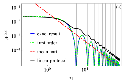
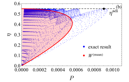
Figure 4: (a) The extra work for the adiabatic process $1\rightarrow 2$ with the special protocol $\tilde{\lambda}_{s}$ by Eq (26). The black curve presents the exact extra work in the previous linear protocol for comparing. The vertical gray-dashed line shows the extra work approaches zero at the specific control time. (b) The reachable power and efficiency with the special protocol. The same parameters are chosen in Fig. 3.

Figure 4(a) presents the first-order adiabatic extra work (the green-dashdotted curve), the mean extra work (the red-dashed line) and the exact one (the blue-solid curve) for the designed protocol by Eq. (26). The extra work for the linear protocol (the black-solid curve) is plotted for comparison. The dynamical phase of the special protocol is $\tilde{\phi}(1)=0.531$, obtained by Eq. (43) in the Appendix A. Hence, the extra work approaches zero at the specific control time $\tau=n\pi/\tilde{\phi}(1)=n\times 5.92,\,n=1,2,...$, shown as the vertical gray-dashed line.

Figure 4(b) presents the constraint relation between the efficiency and the power for the special protocol. When the control time of the two adiabatic processes is chosen as the specific control time $\tau=n\pi/\tilde{\phi}(1)$, the efficiency approaches to the quasi-static efficiency $\eta^{\mathrm{adi}}=0.551$ (the horizontal black-dashed line). For the specific control time $\tau_{1}=\tau_{3}=5.92$, the heat engine gains large power with the quasi-static efficiency, marked with the black point. Compared to the linear protocol, the quantum Otto engine with the special protocol attains larger maximum power and the higher efficiency.

By optimizing the control time of the quantum adiabatic processes, the oscillating extra work can be utilized to improve the maximum power and the efficiency for the finite-time Otto engine. In the next section, we continue to study the effect of similar oscillation of the extra work on the Otto cycle with quantum harmonic oscillator.

IV Quantum Harmonic Otto Engine

Another system with simple energy level structure is the quantum harmonic oscillator, which has been widely studied as a prototype of the quantum Otto engine (Insinga et al., 2016; Kosloff and Rezek, 2017; Deffner, 2018). The technique of shortcut to adiabaticity has been applied to ameliorate the quantum harmonic Otto engine (Deng et al., 2013; Chen et al., 2010; Abah and Lutz, 2018; Çakmak and Özgür E. Müstecaplıoğlu, 2019). Here, we consider a generic finite-time adiabatic process described by the time-dependent Hamiltonian

$$H=-\frac{1}{2M}\frac{\partial^{2}}{\partial x^{2}}+\frac{1}{2}M\omega^{2}x^{2}.$$ (27)

The frequency $\omega=\omega(t),\,t\in[0,\tau]$ serves as the tuning parameter in the finite-time adiabatic process. The wave function of the instantaneous eigenstate is

$$\left\langle x\left|n(t)\right.\right\rangle=N_{n}\exp(-\frac{1}{2}M\omega x^{2})H_{n}(\sqrt{M\omega}x),$$ (28)

with the corresponding instantaneous eigen-energy $E_{n}(t)=(n+1/2)\omega(t)$. $H_{n}(\xi)=(-1)^{n}\exp(\xi^{2})\partial^{n}/\partial\xi^{n}[\exp(-\xi^{2})]$ denotes the Hermite polynomial with the order $n$, and $N_{n}=\left(\sqrt{M\omega}/\sqrt{\pi}2^{n}n!\right)^{1/2}$ is the normalized factor.

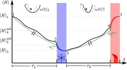
Figure 5: Finite-time Otto cycle of the quantum harmonic oscillator. The frequency $\omega(t)$ of the oscillator is modulated in the finite-time adiabatic process.

Figure 5 illustrates the finite-time quantum harmonic Otto cycle. Similar to the Otto cycle of the two-level system, the work is performed in two adiabatic processes $1\rightarrow 2$ and $3\rightarrow 4$, while the system exchanges the heat with the hot source (cold sink) and reaches equilibrium in the isochoric process $4\rightarrow 1$ ($2\rightarrow 3$).

In the two adiabatic process $1\rightarrow 2$ and $3\rightarrow 4$, the initial state is the thermal state $\rho(0)=\sum_{n=0}^{\infty}p_{n}\left|n(0)\right\rangle\left\langle n(0)\right|$ with the distribution $p_{n}=2\sinh(\beta\omega(0)/2)\exp[-\beta(n+1/2)\omega(0)].$ The density matrix at any time $t$ during the evolution is $\rho(t)=\sum_{n=0}^{\infty}p_{n}\left|\psi_{n}(t)\right\rangle\left\langle\psi_{n}(t)\right|$. Here, the state $\left|\psi_{n}(t)\right\rangle,\,n=0,1,2...$ obeys the Schrodinger equation $i\partial_{t}\left|\psi_{n}(t)\right\rangle=H(t)\left|\psi_{n}(t)\right\rangle,$with the initial condition $\left|\psi_{n}(0)\right\rangle=\left|n(0)\right\rangle$. Similar to Eq. (9), we rewrite the state under the instantaneous diagonal basis

$$\left|\psi_{n}(t)\right\rangle=\sum_{m}c_{nm}(t)e^{-i(m+\frac{1}{2})\varphi(t)}\left|n(t)\right\rangle,$$ (29)

with the dynamical phase $\varphi(t)=\int_{0}^{t}\omega(t^{\prime})dt^{\prime}$. The differential equation of $c_{nm}(t)$ is obtained in Appendix B.

To evaluate the finite-time effect of the quantum adiabatic process, we consider a protocol $\tilde{\omega}(s)=\omega(s\tau)$ with adjustable control time $\tau$, with the instantaneous energy as $\tilde{E}_{n}(s)=E_{n}(s\tau)$. We rewrite the work into the quasi-static work and the extra work as Eq. (2). The quasi-static work with infinite control time $\tau\rightarrow\infty$ is

$$W^{\mathrm{adi}}=\sum_{n=0}^{\infty}p_{n}\left[\tilde{E}_{n}(1)-\tilde{E}_{n}(0)\right],$$ (30)

while extra work in finite-time adiabatic process is

$$W^{\mathrm{(ex)}}(\tau)=\sum_{n,m=0}^{\infty}p_{n}\left|c_{nm}(\tau)\right|^{2}\left[\tilde{E}_{m}(1)-\tilde{E}_{n}(1)\right].$$ (31)

Similar to Eq. (21), the asymptotic amplitude at long control time is given by the first-order adiabatic approximation

$$c_{n,n+2}^{[1]}(\tau) =-i\frac{\sqrt{(n+1)(n+2)}}{8\tau}\left[\frac{\tilde{\omega}^{\prime}(1)}{\tilde{\omega}(1)^{2}}e^{2i\tau\tilde{\varphi}\left(1\right)}-\frac{\tilde{\omega}^{\prime}(0)}{\tilde{\omega}(0)^{2}}\right],$$ (32)

and

$$c_{n,n-2}^{[1]}(\tau)=-i\frac{\sqrt{n(n-1)}}{8\tau}\left[\frac{\tilde{\omega}^{\prime}(1)}{\tilde{\omega}(1)^{2}}e^{-2i\tau\tilde{\varphi}\left(1\right)}-\frac{\tilde{\omega}^{\prime}(0)}{\tilde{\omega}(0)^{2}}\right],$$ (33)

where the dynamical phase factor is $\tilde{\varphi}(1)=\int_{0}^{1}\tilde{\omega}(s)ds$. The derivation of Eqs. (32) and (33) is given in Appendix B. The terms $c_{nm}^{[1]}(\tau),\,m\neq n,\,n\pm 2$ are all zero in the first-order adiabatic approximation. According to Eq. (3), the asymptotic extra work at long control time by Eq. (31) is divided into the mean one

$$W^{\mathrm{(mean)}}(\tau)=\frac{\tilde{\omega}(1)}{8\tau^{2}}\left[\frac{\tilde{\omega}^{\prime}(0)^{2}}{\tilde{\omega}(0)^{4}}+\frac{\tilde{\omega}^{\prime}(1)^{2}}{\tilde{\omega}(1)^{4}}\right]\sum_{n=0}^{\infty}(n+\frac{1}{2})p_{n},$$ (34)

and the oscillating one

$$W^{\mathrm{(osc)}}(\tau)=-\frac{\cos\left[2\tau\tilde{\varphi}(1)\right]}{4\tau^{2}}\frac{\omega^{\prime}(0)\tilde{\omega}^{\prime}(1)}{\omega(0)^{2}\tilde{\omega}(1)}\sum_{n=0}^{\infty}(n+\frac{1}{2})p_{n}.$$ (35)

The exact result of the extra work is obtained from the numerical calculation of the non-adiabatic factor with an auxiliary differential equation (Chen et al., 2010; Abah et al., 2012). The detail is shown in Appendix B.

We calculate the net work $W_{\mathrm{T}}^{\mathrm{adi}}$ and the heat $Q_{\mathrm{h}}^{\mathrm{adi}}$ for the quasi-static Otto cycle. Since the population on each state remains unchanged during the quantum adiabatic processes, the internal energy of the four states follows as $\left\langle H\right\rangle_{1}=\coth\left(\beta_{h}\omega_{0}/2\right)\omega_{0}/2$, $\left\langle H\right\rangle_{2}^{\mathrm{adi}}=\coth\left(\beta_{h}\omega_{0}/2\right)\omega_{1}/2$, $\left\langle H\right\rangle_{3}=\coth\left(\beta_{c}\omega_{1}/2\right)\omega_{1}/2$, and $\left\langle H\right\rangle_{4}^{\mathrm{adi}}=\coth\left(\beta_{c}\omega_{1}/2\right)\omega_{0}/2$. The net work of the quasi-static cycle is

$$W_{\mathrm{T}}^{\mathrm{adi}} =\frac{\omega_{0}-\omega_{1}}{2}\left[\coth\left(\frac{\beta_{\mathrm{h}}\omega_{0}}{2}\right)-\coth\left(\frac{\beta_{\mathrm{c}}\omega_{1}}{2}\right)\right].$$ (36)

The heat absorbed from the hot source is

$$Q_{\mathrm{h}}^{\mathrm{adi}}=\omega_{0}\left[\coth\left(\frac{\beta_{\mathrm{h}}\omega_{0}}{2}\right)-\coth\left(\frac{\beta_{\mathrm{c}}\omega_{1}}{2}\right)\right].$$ (37)

We first adopt the linear protocol $\tilde{\omega}_{l}(s)=\tilde{\omega}(0)+[\tilde{\omega}(1)-\tilde{\omega}(0)]s$ for the finite-time adiabatic process. We set the parameters as $\omega_{0}=2,\,\omega_{1}=1,$ and $M=1$, and choose the temperature for the hot source and cold sink as $T_{\mathrm{h}}=5$ and $T_{\mathrm{c}}=2$ respectively.

In Fig. 6(a), we compare the first-order result of extra work with the exact numerical result for the adiabatic process $1\rightarrow 2$ with $\tilde{\omega}(0)=\omega_{0}$ and $\tilde{\omega}(1)=\omega_{1}$. The first-order adiabatic result (the green-dashdotted curve) matches with the exact numerical result (the blue curve) at long control time. The extra work decreases with oscillation when increasing the control time $\tau_{1}$, retaining the quantum adiabatic limit with infinite control time. Neglecting the oscillation, the extra work satisfies the $\mathcal{C}/\tau^{2}$ scaling (the red dashed line). Figure 6(b) shows the constraint relation between the efficiency and the power for the finite-time quantum harmonic Otto engine. The results are similar to the two-level Otto engine: the oscillating extra work can be utilized to obtain higher maximum power with higher efficiency.

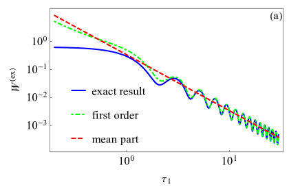
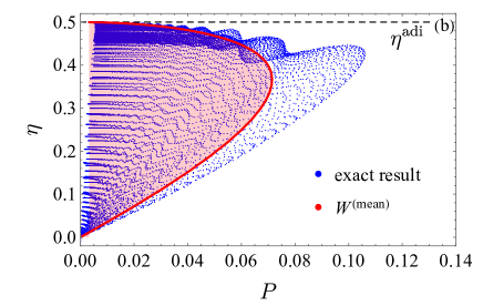
Figure 6: (a) The extra work in the adiabatic process $1\rightarrow 2$ with the linear protocol $\tilde{\omega}_{l}$. The parameter is chosen as $\omega_{0}=2,\,\omega_{1}=1,$ and $M=1$, with the temperatures $T_{\mathrm{h}}=5$ and $T_{\mathrm{c}}=2$. (b) the reachable power and efficiency for the quantum harmonic Otto engine.

To reduce the extra work in the finite-time adiabatic process at the given control time $\tau$, we consider a special protocol (Deng et al., 2016) given by

$$\tilde{\omega}_{s}(s)=\frac{\tilde{\omega}(0)}{\left[\frac{\tilde{\omega}(0)}{\tilde{\omega}(1)}-1\right]s+1},$$ (38)

where $\tilde{\omega}^{\prime}(s)/\tilde{\omega}(s)^{2}=1/\tilde{\omega}(0)-1/\tilde{\omega}(1)$ is a constant. In this special protocol, the extra work by the sum of Eqs (34) and (35) can approach zero at the specific control time $\tau=n\pi/\tilde{\varphi}(1),\,n=1,2,...$, with the dynamical phase $\tilde{\varphi}(1)=[\ln(\tilde{\omega}(0))-\ln(\tilde{\omega}(1))]/[1/\tilde{\omega}(1)-1/\tilde{\omega}(0)]$.

Figure 7 shows the results for the special protocol, with the same parameters chosen in Fig. 6. Figure 7(a) presents the first-order result (green-dashdotted curve) and the exact numerical result (blue-solid curve) of the extra work, with the exact result of the linear protocol shown as the black-solid curve for comparing. Figure 7(a) clearly shows that the extra work is smaller compared to that of the linear protocol for most control time $\tau$, and can approach zero at the specific control time.

Figure 7(b) shows the constraint between the efficiency and the power for the special protocol. When the control time of the two adiabatic processes is chosen as the specific control time $\tau=n\pi/\tilde{\varphi}(1)=n\pi/(2\ln 2),\,n=1,2,...$, the efficiency approaches to the one of the quasi-static Otto cycle (the horizontal black-dashed line). For the specific control time $\tau_{1}=\tau_{3}=\pi/(2\ln 2)$, the heat engine gains large power with the quasi-static efficiency, located as the black point. Compared to the linear protocol in Fig. 6(b), the quantum Otto engine with the special protocol attains larger maximum power and the higher efficiency.

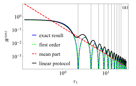
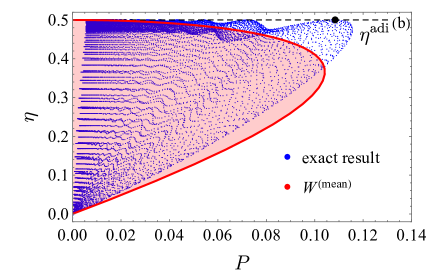
Figure 7: (a) the extra work for the adiabatic process $1\rightarrow 2$ with the special protocol $\tilde{\omega}_{s}$ with different control time $\tau_{1}$. The vertical gray-dashed line shows the extra work approaches zero at the specific control time. (b) the reachable power and efficiency for the quantum harmonic Otto engine. All the parameters are chosen the same in Fig. 6.

V Conclusion

In this paper, we study the effect of the oscillating extra work on both efficiency and output power for the quantum system with simple energy-level structure, e. g. the two-level system and the quantum harmonic oscillator. We conclude that the oscillating property of the extra work can be utilized to obtain higher maximum power and higher efficiency at the maximum power for the finite-time quantum Otto engine by elaborately controlling the finite-time adiabatic processes.

We design special control schemes for the finite-time adiabatic process, where the extra work approaches zero at the specific control time. By adopting the special protocol in the finite-time Otto engine, the engines can be optimized to approach the quasi-static efficiency $\eta^{\mathrm{adi}}$ with non-zero output power in finite-time Otto cycle.

Note: Upon finishing the current paper, we notice the implement of quantum Otto cycle in experiment (Peterson et al., ; de Assis et al., 2019), where the experimental result (Peterson et al., ) clearly shows the oscillation in power and efficiency with the increasing control time. An analytical result of efficiency and power can be obtained at long control time with our general formalism to match the numerical and experimental results in Ref. (Peterson et al., ).

Appendix A The Two-level system

In this Appendix, we give the derivation of the asymptotic amplitude to the first-order adiabatic approximation by Eq. (21). Representing the amplitude $b_{nl}(s)=c_{nl}(\tau s)$ with the rescaled time parameter $s$, Eqs. (17) and (18) are rewritten as

$$\frac{\mathrm{d}}{\mathrm{d}s}b_{ng} =e^{-2i\tau\tilde{\phi}(s)}\frac{\sin\left|\theta\right|}{2\tilde{\Lambda}(s){}^{2}}\frac{\mathrm{d}\tilde{\lambda}}{\mathrm{d}s}b_{ne}$$ (39)

$$\frac{\mathrm{d}}{\mathrm{d}s}b_{ne} =-e^{2i\tau\tilde{\phi}(s)}\frac{\sin\left|\theta\right|}{2\tilde{\Lambda}(s){}^{2}}\frac{\mathrm{d}\tilde{\lambda}}{\mathrm{d}s}b_{ng}.$$ (40)

According to Ref. (Chen et al., ), the solution to the first order of adiabatic approximation is carried out as

$$b_{ge}^{[1]}(s) =\frac{i\sin\left|\theta\right|}{4\epsilon\tau}\left[\frac{\tilde{\lambda}^{\prime}(s)e^{2i\tau\tilde{\phi}(s)}}{\tilde{\Lambda}(s){}^{3}}-\frac{\tilde{\lambda}^{\prime}(0)}{\tilde{\Lambda}(0){}^{3}}\right],$$ (41)

$$b_{eg}^{[1]}(s) =\frac{i\sin\left|\theta\right|}{4\epsilon\tau}\left[\frac{\tilde{\lambda}^{\prime}(s)e^{-2i\tau\tilde{\phi}(s)}}{\tilde{\Lambda}(s){}^{3}}-\frac{\tilde{\lambda}^{\prime}(0)}{\tilde{\Lambda}(0){}^{3}}\right].$$ (42)

The amplitude at the end of the adiabatic process by Eq. (21) follows immediately $c_{ge}^{[1]}(\tau)=b_{ge}^{[1]}(1)$.

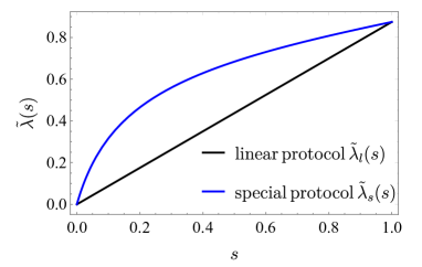
Figure 8: Two protocols for the two-level system, the lower black line for the linear protocol $\tilde{\lambda}_{l}$ and the upper blue curve for the special protocol $\tilde{\lambda}_{s}$. The parameters are chosen as $\tilde{\lambda}(0)=0.1,\,\tilde{\lambda}(1)=0.8,\,\theta=0.4$.

Next, we give the explicit result for the special protocol $\tilde{\lambda}_{s}(s)$. To allow the extra work approach zero at the specific control time, we design a special protocol by setting $\tilde{\lambda^{\prime}}(s)/\tilde{\Lambda}(s){}^{3}=C$ as a constant at any moment during the adiabatic process. The constant $C$ is determined by the initial $\tilde{\lambda}(0)$ and final value $\tilde{\lambda}(1)$. Together with the initial and final condition, we obtain the implicit function by Eq. (26). In Fig. 8, we compare the special protocol $\tilde{\lambda}_{s}$ with the linear protocol $\tilde{\lambda}_{l}$, with the chosen parameters $\theta=0.4,\,\epsilon=1,\,\tilde{\lambda}(0)=0.1,\,\tilde{\lambda}(1)=0.8$. For the the special protocol, we obtain the dynamical phase at the end of the process as

$$\tilde{\phi}(1)=\frac{\epsilon\sin(\theta)\left[\arctan\left(\frac{(1+\tilde{\lambda}(1))\tan\frac{\theta}{2}}{1-\tilde{\lambda}(1)}\right)-\arctan\left(\frac{(1+\tilde{\lambda}(0))\tan\frac{\theta}{2}}{1-\tilde{\lambda}(0)}\right)\right]}{\frac{\tilde{\lambda}(1)-\cos\theta}{\sqrt{\tilde{\lambda}(1)^{2}-2\tilde{\lambda}(1)\cos\theta+1}}-\frac{\tilde{\lambda}(0)-\cos\theta}{\sqrt{\text{$\tilde{\lambda}$(0)}^{2}-2\tilde{\lambda}(0)\cos\theta+1}}}.$$ (43)

The extra work approaches zero at the special control time $\tau=n\pi/\tilde{\phi}\left(1\right),\,n=1,2...$

Appendix B Time-dependent Harmonic Oscillator

In this appendix, we give the results of the time-dependent harmonic oscillator, including the first-order adiabatic result and the method for numerical calculation.

Following the method in Ref (Chen et al., ), the differential equation of the amplitude $c_{nm}(t)$ follows from the Schrodinger equation as

$$\frac{d}{dt}c_{nl}(t)+c_{nl}(t)\left\langle l\left|\dot{l}\right.\right\rangle+\sum_{m\neq l}c_{nm}(t)e^{-i(m-l)\varphi(t)}\left\langle l\left|\dot{m}\right.\right\rangle=0,$$ (44)

where $\left|l\right\rangle=\left|l(t)\right\rangle$ is the instantaneous eigenstate of the time-dependent harmonic oscillator. We rewrite the equation with the rescaled time parameter $s$ as

$$\frac{d}{ds}b_{nl}(s)+b_{nl}(s)\left\langle\tilde{l}\left|\frac{\partial}{\partial s}\right|\tilde{l}\right\rangle+\sum_{m\neq l}b_{nm}(s)e^{-i\tau(m-l)\tilde{\varphi}(s)}\left\langle\tilde{l}\left|\frac{\partial}{\partial s}\right|\tilde{m}\right\rangle=0,$$ (45)

with $\left|\tilde{l}\right\rangle=\left|l(s\tau)\right\rangle$. With the property of Hermite polynomial $H_{n}(\xi),$ we obtain the derivative of the instantaneous eigenstate by Eq. (28) as

$$\left\langle\tilde{m}\right|\frac{\partial}{\partial s}\left|\tilde{n}\right\rangle=\frac{\tilde{\omega}^{\prime}(s)}{4\tilde{\omega}(s)}\left(-\sqrt{(n+1)(n+2)}\delta_{m,n+2}+\sqrt{n(n-1)}\delta_{m,n-2}\right).$$ (46)

The terms $\left\langle\tilde{m}\right|\frac{\partial}{\partial s}\left|\tilde{n}\right\rangle$ with $m\neq n\pm 2$ are all zero.

According to Ref. (Chen et al., ), we obtain the solution to the first order of adiabatic approximation as

$$b_{n,n+2}^{[1]}(s) =-i\frac{\sqrt{(n+1)(n+2)}}{8\tau}\left(\frac{\tilde{\omega}^{\prime}(s)}{\tilde{\omega}(s)^{2}}e^{2i\tau\tilde{\varphi}\left(s\right)}-\frac{\tilde{\omega}^{\prime}(0)}{\tilde{\omega}(0)^{2}}\right),$$ (47)

and

$$b_{n,n-2}^{[1]}(s)=-i\frac{\sqrt{n(n-1)}}{8\tau}\left(\frac{\tilde{\omega}^{\prime}(s)}{\tilde{\omega}(s)^{2}}e^{-2i\tau\tilde{\varphi}\left(s\right)}-\frac{\tilde{\omega}^{\prime}(0)}{\tilde{\omega}(0)^{2}}\right).$$ (48)

The diagonal term to the first order of adiabatic approximation is $b_{n,n}^{[1]}(s)=1$ (Chen et al., ). The terms $b_{n,m}^{[1]}(s)=0$$,\,m\neq n,\,n\pm 2$ are all zero since $\left\langle\widetilde{m}\right|\frac{\partial}{\partial s}\left|\tilde{n}\right\rangle=0$. The amplitude at the end of the adiabatic process by Eqs. (32,33) follows as $c_{n,n\pm 2}^{[1]}(\tau)=b_{n,n\pm 2}^{[1]}(1)$.

In Ref. (Chen et al., 2010), the exact result of the internal energy during the finite-time adiabatic process is described by the non-adiabatic factor $\mathscr{N}(t)$ as

$$\left\langle H(\omega(t))\right\rangle=\frac{\omega(t)}{2}\mathscr{N}(t)\coth\left[\frac{\beta\omega(0)}{2}\right].$$ (49)

The non-adiabatic factor $\mathscr{N}(t)$ is determined by a scalar $c(t)$ as

$$\mathscr{N}(t)=\frac{\left[\dot{c}(t)\right]^{2}+\left[\omega(t)\right]^{2}\left[c(t)\right]^{2}+\frac{\left[\omega(0)\right]^{2}}{\left[c(t)\right]^{2}}}{2\omega(t)\omega(0)},$$ (50)

where $c(t)$ satisfies the differential equation

$$\text{$\ddot{c}(t)+\omega(t)^{2}c(t)=\frac{\omega(0)^{2}}{c(t)^{3}}$},$$ (51)

with the initial condition $c(0)=1,\,c^{\prime}(0)=0$.

With Eq. (49), the work during the finite-time adiabatic process is rewritten with $\mathscr{N}(t)$ as $W(\tau)=\frac{\omega(\tau)}{2}\mathscr{N}(\tau)\coth\left(\frac{\beta\omega(0)}{2}\right)-\frac{\omega(0)}{2}\coth\left(\frac{\beta\omega(0)}{2}\right)$. Correspondingly, the quasi-static work is

$$W^{\mathrm{adi}}=\frac{\omega(\tau)-\omega(0)}{2}\coth\left(\frac{\beta\omega(0)}{2}\right),$$ (52)

and the extra work is

$$W^{(\mathrm{ex})}(\tau)=\frac{\omega(\tau)}{2}\left[\mathscr{N}(\tau)-1\right]\coth\left(\frac{\beta\omega(0)}{2}\right).$$ (53)

It is verified $\mathscr{N}(\tau)\geq 1$, which approach $1$ for infinite control time $\tau\rightarrow\infty$. The difference $\mathscr{N}(\tau)-1$ describes the non-adiabatic effect, and does not depend on the initial inverse temperature $\beta$. Substituting Eq. (53) into Eqs. (4) and (5), we rewrite the output power

$$P^{\mathrm{h}}=\frac{\left[\omega_{0}-\omega_{1}\mathscr{N}_{1}(\tau_{1})\right]\coth\left(\frac{\beta_{\mathrm{h}}\omega_{0}}{2}\right)+\left[\omega_{1}-\omega_{0}\mathscr{N}_{3}(\tau_{3})\right]\coth\left(\frac{\beta_{\mathrm{c}}\omega_{1}}{2}\right)}{2(\tau_{1}+\tau_{3})},$$ (54)

and the corresponding efficiency

$$\eta^{\mathrm{h}}=1-\frac{\omega_{1}\left[\mathscr{N}_{1}(\tau_{1})\coth\left(\frac{\beta_{\mathrm{h}}\omega_{0}}{2}\right)-\coth\left(\frac{\beta_{\mathrm{c}}\omega_{1}}{2}\right)\right]}{\omega_{0}\left[\coth\left(\frac{\beta_{\mathrm{h}}\omega_{0}}{2}\right)-\mathscr{N}_{3}(\tau_{3})\coth\left(\frac{\beta_{\mathrm{c}}\omega_{1}}{2}\right)\right]},$$ (55)

where $\mathscr{N}_{1}(\tau_{1})$ and $\mathscr{N}_{3}(\tau_{3})$ denote the non-adiabatic factors for the two finite-time adiabatic processes. In the numerical calculation, we first choose different control time to obtain the exact result of the non-adiabatic factor $\mathscr{N}_{i}(\tau_{i}),\,i=1,3$ for the two finite-time adiabatic processes by solving Eq. (51) numerically. Then, we use Eqs. (54) and (55) to calculate the exact power and efficiency, respectively.

References

- Maruyama et al. (2009) K. Maruyama, F. Nori, and V. Vedral, Rev. Mod. Phys. 81, 1 (2009).
- Esposito et al. (2009) M. Esposito, U. Harbola, and S. Mukamel, Rev. Mod. Phys. 81, 1665 (2009).
- Campisi et al. (2011) M. Campisi, P. Hänggi, and P. Talkner, Rev. Mod. Phys. 83, 771 (2011).
- Strasberg et al. (2017) P. Strasberg, G. Schaller, T. Brandes, and M. Esposito, Phys. Rev. X 7, 021003 (2017).
- Vinjanampathy and Anders (2016) S. Vinjanampathy and J. Anders, Contemp. Phys. 57, 545 (2016).
- Scully et al. (2003) M. O. Scully, S. Zubairy, G. S. Agarwal, and H. Walther, Science 299, 862 (2003).
- Quan et al. (2006) H. T. Quan, P. Zhang, and C. P. Sun, Phys. Rev. E 73, 036122 (2006).
- Solinas and Gasparinetti (2016) P. Solinas and S. Gasparinetti, Phys. Rev. A 94, 052103 (2016).
- Francica et al. (2019) G. Francica, J. Goold, and F. Plastina, Phys. Rev. E 99, 042105 (2019).
- Benatti et al. (2003) F. Benatti, R. Floreanini, and M. Piani, Phys. Rev. Lett. 91, 070402 (2003).
- Kraus et al. (2008) B. Kraus, H. P. Büchler, S. Diehl, A. Kantian, A. Micheli, and P. Zoller, Phy. Rev. A 78, 042307 (2008).
- Altintas et al. (2014) F. Altintas, A. U. C. Hardal, and Özgür E. Müstecaplıoğlu, Phys. Rev. E 90, 032102 (2014).
- (13) A. Tavakoli, G. Haack, N. Brunner, and J. B. Brask, “Autonomous multipartite entanglement engines,” 1906.00022v1 .
- Jaramillo et al. (2016) J. Jaramillo, M. Beau, and A. del Campo, New J. Phys. 18, 075019 (2016).
- Ma et al. (2017) Y.-H. Ma, S.-H. Su, and C.-P. Sun, Phys. Rev. E 96, 022143 (2017).
- Bengtsson et al. (2018) J. Bengtsson, M. N. Tengstrand, A. Wacker, P. Samuelsson, M. Ueda, H. Linke, and S. Reimann, Phys. Rev. Lett. 120, 100601 (2018).
- Chen et al. (2018) J. Chen, H. Dong, and C.-P. Sun, Phys. Rev. E 98, 062119 (2018).
- Curzon and Ahlborn (1975) F. L. Curzon and B. Ahlborn, Am. J. Phys 43, 22 (1975).
- Salamon and Berry (1983) P. Salamon and R. S. Berry, Phys. Rev. Lett. 51, 1127 (1983).
- Esposito et al. (2010) M. Esposito, R. Kawai, K. Lindenberg, and C. VandenBroeck, Phys. Rev. Lett. 105, 150603 (2010).
- Andresen (2011) B. Andresen, Angew. Chem. Int. Ed. 50, 2690 (2011).
- Whitney (2014) R. S. Whitney, Phys. Rev. Lett. 112, 130601 (2014).
- Dann et al. (2019) R. Dann, A. Tobalina, and R. Kosloff, Phys. Rev. Lett. 122, 250402 (2019).
- Quan et al. (2007) H. T. Quan, Y. X. Liu, C. P. Sun, and F. Nori, Phys. Rev. E 76, 031105 (2007).
- Tu (2008) Z. C. Tu, J. Phys. A: Math. Theor. 41, 312003 (2008).
- Rutten et al. (2009) B. Rutten, M. Esposito, and B. Cleuren, Phys. Rev. B 80, 235122 (2009).
- Alecce et al. (2015) A. Alecce, F. Galve, N. L. Gullo, L. Dell’Anna, F. Plastina, and R. Zambrini, New J. Phys. 17, 075007 (2015).
- Shiraishi et al. (2016) N. Shiraishi, K. Saito, and H. Tasaki, Phys. Rev. Lett. 117, 190601 (2016).
- Deffner (2018) S. Deffner, Entropy 20, 875 (2018).
- Schmiedl and Seifert (2007) T. Schmiedl and U. Seifert, EPL (Europhysics Letters) 81, 20003 (2007).
- Cavina et al. (2017) V. Cavina, A. Mari, and V. Giovannetti, Phys. Rev. Lett. 119, 050601 (2017).
- Ryabov and Holubec (2016) A. Ryabov and V. Holubec, Phys. Rev. E 93, 050101(R) (2016).
- Long and Liu (2016) R. Long and W. Liu, Phys. Rev. E 94, 052114 (2016).
- Holubec and Ryabov (2016) V. Holubec and A. Ryabov, J. Stat. Mech: Theory Exp. 2016, 073204 (2016).
- Ma et al. (2018a) Y.-H. Ma, D. Xu, H. Dong, and C.-P. Sun, Phys. Rev. E 98, 022133 (2018a).
- Ma et al. (2018b) Y.-H. Ma, D. Xu, H. Dong, and C.-P. Sun, Phys. Rev. E 98, 042112 (2018b).
- Abah et al. (2012) O. Abah, J. Roßnagel, G. Jacob, S. Deffner, F. Schmidt-Kaler, K. Singer, and E. Lutz, Phys. Rev. Lett. 109, 203006 (2012).
- Roßnagel et al. (2014) J. Roßnagel, O. Abah, F. Schmidt-Kaler, K. Singer, and E. Lutz, Phys. Rev. Lett. 112, 030602 (2014).
- Karimi and Pekola (2016) B. Karimi and J. P. Pekola, Phys. Rev. B 94, 184503 (2016).
- Insinga et al. (2016) A. Insinga, B. Andresen, and P. Salamon, Phys. Rev. E 94, 012119 (2016).
- Campisi and Fazio (2016) M. Campisi and R. Fazio, Nat. Commun. 7, 11895 (2016).
- Kosloff and Rezek (2017) R. Kosloff and Y. Rezek, Entropy 19, 136 (2017).
- Erdman et al. (2018) P. A. Erdman, V. Cavina, R. Fazio, F. Taddei, and V. Giovannetti, “Maximum power and corresponding efficiency for two-level quantum heat engines and refrigerators,” (2018), arXiv:1812.05089 .
- (44) T. Denzler and E. Lutz, “Efficiency fluctuations of a quantum otto engine,” 1907.02566v1 .
- Chen et al. (2010) X. Chen, A. Ruschhaupt, S. Schmidt, A. del Campo, D. Guéry-Odelin, and J. G. Muga, Phys. Rev. Lett. 104, 063002 (2010).
- Deng et al. (2013) J. Deng, Q. hai Wang, Z. Liu, P. Hänggi, and J. Gong, Phys. Rev. E 88, 062122 (2013).
- Abah and Lutz (2018) O. Abah and E. Lutz, Phys. Rev. E 98, 032121 (2018).
- Deng et al. (2018) S. Deng, A. Chenu, P. Diao, F. Li, S. Yu, I. Coulamy, A. del Campo, and H. Wu, Sci. Adv. 4, eaar5909 (2018).
- Çakmak and Özgür E. Müstecaplıoğlu (2019) B. Çakmak and Özgür E. Müstecaplıoğlu, Phys. Rev. E 99, 032108 (2019).
- Chotorlishvili et al. (2016) L. Chotorlishvili, M. Azimi, S. Stagraczyński, Z. Toklikishvili, M. Schüler, and J. Berakdar, Phys. Rev. E 94, 032116 (2016).
- Su et al. (2018) S. Su, J. Chen, Y. Ma, J. Chen, and C. Sun, Chin. Phys. B 27, 060502 (2018).
- Sun (1988) C.-P. Sun, J. Phys. A: Math. Gen. 21, 1595 (1988).
- Wilczek and Shapere (1989) F. Wilczek and A. Shapere, Geometric Phases in Physics (WORLD SCIENTIFIC, 1989).
- Sun (1990) C.-P. Sun, Phys. Rev. D 41, 1318 (1990).
- Rigolin et al. (2008) G. Rigolin, G. Ortiz, and V. H. Ponce, Phys. Rev. A 78, 052508 (2008).
- (56) J.-F. Chen, C.-P. Sun, and H. Dong, “Achieve higher efficiency at maximum power with finite-time quantum otto cycle,” 1904.12128v1 .
- Deng et al. (2016) S. Deng, Z.-Y. Shi, P. Diao, Q. Yu, H. Zhai, R. Qi, and H. Wu, Science 353, 371 (2016).
- (58) J. P. S. Peterson, T. B. Batalhão, M. Herrera, A. M. Souza, R. S. Sarthour, I. S. Oliveira, and R. M. Serra, “Experimental characterization of a spin quantum heat engine,” 1803.06021v1 .
- de Assis et al. (2019) R. J. de Assis, T. M. de Mendonça, C. J. Villas-Boas, A. M. de Souza, R. S. Sarthour, I. S. Oliveira, and N. G. de Almeida, Phys. Rev. Lett. 122, 240602 (2019).