Double Bayesian Smoothing as Message Passing

Abstract

Recently, a novel method for developing filtering algorithms, based on the interconnection of two Bayesian filters and called double Bayesian filtering, has been proposed. In this manuscript we show that the same conceptual approach can be exploited to devise a new smoothing method, called double Bayesian smoothing. A double Bayesian smoother combines a double Bayesian filter, employed in its forward pass, with the interconnection of two backward information filters used in its backward pass. As a specific application of our general method, a detailed derivation of double Bayesian smoothing algorithms for conditionally linear Gaussian systems is illustrated. Numerical results for two specific dynamic systems evidence that these algorithms can achieve a better complexity-accuracy tradeoff and tracking capability than other smoothing techniques recently appeared in the literature.

Keywords: Hidden Markov Model, Smoothing, Factor Graph, Particle Filter, Kalman Filter, Sum-Product Algorithm.

I. Introduction

The problem of Bayesian smoothing for a state space model (SSM) concerns the development of recursive algorithms able to estimate the probability density function (pdf) of the model state on a given observation interval, given a batch of noisy measurements acquired over it [1], [2]; the estimated pdf is known as a smoothed or smoothing pdf. Two general methods are available in the literature for recursively calculating smoothing densities; they are known as the forward filtering-backward smoothing recursion (e.g., see [3] and [4]) and the method based on the two-filter smoothing formula (e.g., see [5] and [6]). Both methods are based on the idea that the smoothing densities can be computed by combining the predicted and/or filtered densities generated by a Bayesian filtering method with the statistical information produced in the backward pass by a different filtering method; the latter method is paired with the first one and, in the case of the two-filter smoothing formula, is known as backward information filtering (BIF). Unluckily, closed form solutions for Bayesian smoothing are available for linear Gaussian and linear Gaussian mixture models only [1, 2, 7]. This has motivated the development of various methods based on approximating smoothing densities in different ways. For instance, the use of Gaussian approximations for the smoothing densities and of sigma points techniques for solving moment matching integrals has been investigated in [8, 9, 10]. Another class of methods (usually known as particle smoothers) is based on the exploitation of sequential Monte Carlo techniques, i.e. on approximating smoothing densities through a set of weighted particles (e.g., see [3, 11, 5, 12, 13, 14] and references therein). Recently, substantial attention has been also paid to the development of smoothing algorithms for the class of conditionally linear Gaussian SSMs [15, 16, 17, 18, 19]. In this case, the above mentioned approximate methods can benefit from the so called Rao-Blackwellization technique, i.e. from the marginalisation of the linear substructure of any conditionally linear Gaussian model; this can significantly reduce the overall computational complexity of both sigma-point based Gaussian smoothing [15] and particle smoothing [16, 17, 18, 19] (that is usually known as Rao-Blackwellized particle smoothing, RBPS, in this case).

In this manuscript, we propose a novel general method for the development of computationally efficient particle smoothers. Our method exploits the same conceptual approach illustrated in [20] in the context of Bayesian filtering and dubbed multiple Bayesian filtering. That approach is based on the idea of developing new filtering algorithms by: a) interconnecting multiple heterogeneous Bayesian filters; b) representing the processing accomplished by each Bayesian filter and the exchange of statistical information among distinct filters as a message passing over a proper factor graph. In [20] the exploitation of this approach has been investigated in detail for the case in which two Bayesian filters are interconnected, i.e. dual Bayesian filtering (DBF) is employed. Moreover, it has been shown that accurate and computationally efficient DBF algorithms can be devised if the considered SSM is conditionally linear Gaussian. In this manuscript, we show that, if DBF is employed in the forward pass of a smoothing method, a BIF method, paired with DBF and based on the interconnection of two backward information filters can be devised by following some simple rules. Similarly as DBF, our derivation of such a BIF method, called double backward information filtering (DBIF), is based on a graphical model. Such a graphical model allows us to show that: a) the pdfs computed in DBIF can be represented as messages passed on it; b) all the expressions of the passed messages can be derived by applying the same rule, namely the so called sum-product algorithm (SPA) [21], [22], to it; c) iterative algorithms can be developed in a natural fashion once the cycles it contains have been identified and the order according to which messages are passed on them (i.e., the message scheduling) has been established; d) the statistical information generated by a DBIF algorithm in the backward pass can be easily merged with those produced by its paired DBF technique in the forward pass in order to evaluate the required smoothed pdfs. To exemplify the usefulness of the resulting smoothing method, based on the combination of DBF and DBIF, and called double Bayesian smoothing (DBS), the two DBF algorithms proposed in [20] for the class of conditionally linear Gaussian SSMs are taken into consideration, and the BITF algorithm paired with each of them and a simplified version of it are derived. This leads to the development of four new DBS algorithms, two generating an estimate of the joint smoothing density over the whole observation interval, the other two an estimate of the marginal smoothing densities over the same interval. Our computer simulations for two specific conditionally linear Gaussian SSMs evidence that, in the first case, the derived DBS algorithms perform very closely to the RBPS technique proposed in [18] and to the particle smoothers devised in [19], but at lower computational cost and time. In the second case, instead, two of the devised DBS techniques represent the only technically useful options, thanks to their good tracking capability. In fact, such techniques are able to operate reliably even when their competitors diverge in the forward pass.

It is worth stressing that the technical contribution provided by this manuscript represents a significant advancement with respect to the application of factor graph theory to particle smoothing illustrated in [19]. In fact, in that manuscript, we also focus on conditionally linear Gaussian models, but assume that the forward pass is accomplished by marginalized particle filtering (MPF; also known as Rao-Blackwellized particle filtering); in other words, Bayesian filtering is based on the interconnection of a particle filter with a bank of Kalman filters. In this manuscript, instead, the general method we propose applies to a couple of arbitrary interconnected Bayesian filters. Moreover, the specific smoothing algorithms we derive assume that the forward pass is carried out by a filtering algorithm based on the interconnection of a particle filter with a single extended Kalman filter.

The remaining part of this manuscript is organized as follows. In Section II., a general graphical model, on which the processing accomplished in DBF, DBIF, and DBS is based, is illustrated. In Section III., a specific instance of the graphical model illustrated in the previous section is developed under the assumptions that the filters employed in the forward pass are an extended Kalman filter and a particle filter, and that the considered SSM is conditionally linear Gaussian. Then, the scheduling and the computation of the messages passed over this model are analysed in detail and new DBS algorithms are devised. The differences and similarities between these algorithms and other known smoothing techniques are analysed in Section IV.. A comparison, in terms of accuracy, computational complexity, and execution time, between the proposed techniques and three smoothers recently appeared in the literature, is provided in Section V. for two conditionally linear Gaussian SSMs. Finally, some conclusions are offered in Section VI..

Notations: The same notation as refs. [19, 20] and [23] is adopted.

II. Graphical Model for a Couple of Interconnected Bayesian Information Filters and Message Passing on it

In this manuscript, we consider a discrete-time SSM whose $D-$dimensional hidden state in the $k-$th interval is denoted $\mathbf{x}_{k}\triangleq[x_{0,k},x_{1,k},...,$ $x_{D-1,k}]^{T}$, and whose state update and measurement models are expressed by

$$\mathbf{x}_{k+1}=\mathbf{f}_{k}\left(\mathbf{x}_{k}\right)+\mathbf{w}_{k}$$ (1)

and

$$\mathbf{y}_{k} \triangleq [y_{0,k},y_{1,k},...,y_{P-1,k}]^{T}$$ (2)

$$= \mathbf{h}_{k}\left(\mathbf{x}_{k}\right)+\mathbf{e}_{k},$$

respectively, with $k=1$, $2$, $...$, $T$. Here, $\mathbf{f}_{k}\left(\mathbf{x}_{k}\right)$ ($\mathbf{h}_{k}\left(\mathbf{x}_{k}\right)$) is a time-varying $D-$dimensional ($P-$dimensional) real function, $T$ is the duration of the observation interval and $\mathbf{w}_{k}$ ($\mathbf{e}_{k}$) is the $k-$th element of the process (measurement) noise sequence $\left\{\mathbf{w}_{k}\right\}$ ($\left\{\mathbf{e}_{k}\right\}$); this sequence consists of $D-$dimensional ($P-$dimensional) independent and identically distributed (iid) Gaussian noise vectors, each characterized by a zero mean and a covariance matrix $\mathbf{C}_{w}$ ($\mathbf{C}_{e}$). Moreover, statistical independence between $\left\{\mathbf{e}_{k}\right\}$ and $\{\mathbf{w}_{k}\}$ is assumed.

From a statistical viewpoint, a complete statistical description of the considered SSM is provided by the pdf $f(\mathbf{x}_{1})$ of its initial state, its Markov model $f(\mathbf{x}_{k+1}|\mathbf{x}_{k})$ and its observation model $f(\mathbf{y}_{k}|\mathbf{x}_{k})$ for any $k$; the first pdf is assumed to be known, whereas the last two pdfs can be easily derived from Eq. (1) and Eq. (2), respectively.

In the following, we focus on the problem of developing novel smoothing algorithms and, in particular, algorithms for the estimation of the joint smoothed pdf $f(\mathbf{x}_{1:T}|\mathbf{y}_{1:T})$ (problem P.1) and the sequence of marginal smoothed pdfs $\{f(\mathbf{x}_{k}|\mathbf{y}_{1:T}),\,k=1,2,...,T\}$ (problem P.2); here, $\mathbf{y}_{1:T}\triangleq\left[\mathbf{y}_{1}^{T},\mathbf{y}_{2}^{T},...,\mathbf{y}_{T}^{T}\right]^{T}$ is a $P\cdot T-$dimensional vector. Note that, in principle, once problem P.1 is solved, problem P.2 can be easily tackled; in fact, if the joint pdf $f(\mathbf{x}_{1:T}|\mathbf{y}_{1:T})$ is known, all the posterior pdfs $\{f(\mathbf{x}_{k}|\mathbf{y}_{1:T})\}$ can be evaluated by marginalization.

The development of our smoothing algorithms is mainly based on the graphical approach illustrated in our previous manuscripts [19, Sec. III], [20, Sec. II] and [23, Sec. III] for Bayesian filtering and smoothing. This approach consists in the following steps:

1. The state vector $\mathbf{x}_{k}$ is partitioned in two substates, denoted $\mathbf{x}_{k}^{(1)}$ and $\mathbf{x}_{k}^{(2)}$ and having sizes $D_{1}$ and $D_{2}=D-D_{1}$, respectively. Note that, if $\mathbf{\bar{x}}_{k}^{(i)}$ represents the portion of $\mathbf{x}_{k}$ not included in $\mathbf{x}_{k}^{(i)}$ (with $i=1$ and $2$), our assumptions entail that $\mathbf{\bar{x}}_{k}^{(1)}=\mathbf{x}_{k}^{(2)}$ and $\mathbf{\bar{x}}_{k}^{(2)}=\mathbf{x}_{k}^{(1)}$.

2. A sub-graph that allows to represent both Bayesian filtering and BIF for the substate $\mathbf{x}_{k}^{(i)}$ (with $i=1$ and $2$) as message passing algorithms on it is developed, under the assumption that the complementary substate $\mathbf{\bar{x}}_{k}^{(i)}$ is statistically known. This means that filtered and predicted densities of $\mathbf{x}_{k}^{(i)}$ are represented as messages passed on the edges of this sub-graph and the rules for computing them result from the application of the SPA to it.

3. The two sub-graphs devised in the previous step (one referring to $\mathbf{x}_{k}^{(1)}$, the other one to $\mathbf{x}_{k}^{(2)}$) are interconnected, so that a single graphical model referring to the whole state $\mathbf{x}_{k}$ is obtained.

4. Algorithms for Bayesian filtering and BIF for the whole state $\mathbf{x}_{k}$ are derived by applying the SPA to the graphical model obtained in the previous step.

Let us analyse now the steps 2.-4. in more detail. As far as step 2. is concerned, the sub-graph devised for the substate $\mathbf{x}_{k}^{(i)}$ is based on the same principles illustrated in our manuscripts cited above (in particular, ref. [20]) and is illustrated in Fig. 1. The $k-$th recursion (with $k=1,2,...,T$) of Bayesian filtering for the sub-state $\mathbf{x}_{k}^{(i)}$ is represented as a forward message passing on this factor graph, that involves the Markov model $f(\mathbf{x}_{k+1}^{(i)}|\mathbf{x}_{k}^{(i)},\mathbf{\bar{x}}_{k}^{(i)})$ and the observation model $f(\mathbf{y}_{k}|\mathbf{x}_{k}^{(i)},\mathbf{\bar{x}}_{k}^{(i)})$. This allows to compute the messages $\vec{m}_{\mathrm{fe}1}(\mathbf{x}_{k}^{(i)})$, $\vec{m}_{\mathrm{fe}2}(\mathbf{x}_{k}^{(i)})$ and $\vec{m}_{\mathrm{fp}}(\mathbf{x}_{k+1}^{(i)})$, that convey the first filtered pdf of $\mathbf{x}_{k}^{(i)}$, the second filtered pdf of $\mathbf{x}_{k}^{(i)}$ and the predicted pdf of $\mathbf{x}_{k+1}^{(i)}$, respectively, on the basis of the messages $\vec{m}_{\mathrm{fp}}(\mathbf{x}_{k}^{(i)})$, $m_{\mathrm{ms}}(\mathbf{x}_{k}^{(i)})$ and $m_{\mathrm{pm}}(\mathbf{x}_{k}^{(i)})$; the last three messages represent the predicted pdf of $\mathbf{x}_{k}^{(i)}$ evaluated in the previous (i.e., in the $(k-1)-$th) recursion of Bayesian filtering, and the messages conveying the measurement and the pseudo-measurement information, respectively, available in the $k-$recursion. The considered filtering algorithm requires the availability of the messages $m_{\mathrm{pm}}(\mathbf{x}_{k}^{(i)})$, $m_{\mathrm{mg}1}(\mathbf{\bar{x}}_{k}^{(i)})$, $m_{\mathrm{mg}2}(\mathbf{\bar{x}}_{k}^{(i)})$, that are computed on the basis of external statistical information. The presence of the messages $m_{\mathrm{mg}1}(\mathbf{\bar{x}}_{k}^{(i)})$ and $m_{\mathrm{mg}2}(\mathbf{\bar{x}}_{k}^{(i)})$ is due the fact that the substate $\mathbf{\bar{x}}_{k}^{(i)}$ represents a nuisance state for the considered filtering algorithm; in fact, these messages convey filtered (or predicted) pdfs of $\mathbf{\bar{x}}_{k}^{(i)}$ and are employed to integrate out the dependence of the pdfs $f(\mathbf{y}_{k}|\mathbf{x}_{k}^{(i)},\mathbf{\bar{x}}_{k}^{(i)})$ and $f(\mathbf{x}_{k+1}^{(i)}|\mathbf{x}_{k}^{(i)},\mathbf{\bar{x}}_{k}^{(i)})$, respectively, on $\mathbf{\bar{x}}_{k}^{(i)}$. Note also that these two messages are not necessarily equal, since more refined information about $\mathbf{\bar{x}}_{k}^{(i)}$ could become available after that the message $m_{\mathrm{ms}}(\mathbf{x}_{k}^{(i)})$ has been computed. On the other hand, the message $m_{\mathrm{pm}}(\mathbf{x}_{k}^{(i)})$ conveys the statistical information provided by a pseudo-measurement about $\mathbf{x}_{k}^{(i)}$. In Fig. 1, following [20, Sec. II], it is assumed that the pseudo-measurement $\mathbf{z}_{k}^{(i)}$ is available in the estimation of $\mathbf{x}_{k}^{(i)}$ and that $m_{\mathrm{pm}}(\mathbf{x}_{k}^{(i)})$ represents the pdf of $\mathbf{z}_{k}^{(i)}$ conditioned on $\mathbf{x}_{k}^{(i)}$, that is

$$m_{\mathrm{pm}}\left(\mathbf{x}_{k}^{(i)}\right)\triangleq f\left(\mathbf{z}_{k}^{(i)}\left|\mathbf{x}_{k}^{(i)}\right.\right).$$ (3)

The computation of the messages $\vec{m}_{\mathrm{fe}1}(\mathbf{x}_{k}^{(i)})$, $\vec{m}_{\mathrm{fe}2}(\mathbf{x}_{k}^{(i)})$ and $\vec{m}_{\mathrm{fp}}(\mathbf{x}_{k+1}^{(i)})$ on the basis of the messages $\vec{m}_{\mathrm{fp}}(\mathbf{x}_{k}^{(i)})$, $m_{\mathrm{ms}}(\mathbf{x}_{k}^{(i)})$, $m_{\mathrm{pm}}(\mathbf{x}_{k}^{(i)})$, $m_{\mathrm{mg}1}(\mathbf{\bar{x}}_{k}^{(i)})$ and $m_{\mathrm{mg}2}(\mathbf{\bar{x}}_{k}^{(i)})$ is based on the two simple rules illustrated in [23, Figs. 8-a) and 8-b), p. 1535] and can be summarized as follows. The first and second filtered pdfs (i.e., the first and the second forward estimates) of $\mathbf{x}_{k}^{(i)}$ are evaluated as

$$\vec{m}_{\mathrm{fe}1}\left(\mathbf{x}_{k}^{(i)}\right)=\vec{m}_{\mathrm{fp}}\left(\mathbf{x}_{k}^{(i)}\right)m_{\mathrm{ms}}\left(\mathbf{x}_{k}^{(i)}\right),$$ (4)

and

$$\vec{m}_{\mathrm{fe}2}\left(\mathbf{x}_{k}^{(i)}\right)=\vec{m}_{\mathrm{fe}1}\left(\mathbf{x}_{k}^{(i)}\right)m_{\mathrm{pm}}\left(\mathbf{x}_{k}^{(i)}\right),$$ (5)

respectively, where

$$m_{\mathrm{ms}}\left(\mathbf{x}_{k}^{(i)}\right)\triangleq\int f\left(\mathbf{y}_{k}\left|\mathbf{x}_{k}^{(i)},\mathbf{\bar{x}}_{k}^{(i)}\right.\right)\,m_{\mathrm{mg}1}\left(\mathbf{\bar{x}}_{k}^{(i)}\right)\,d\mathbf{\bar{x}}_{k}^{(i)}$$ (6)

and $m_{\mathrm{pm}}(\mathbf{x}_{k}^{(i)})$ is defined in Eq. (3). Equations (4)-(6) describe the processing accomplished in the measurement update of the considered recursion. This is followed by the time update, in which the new predicted pdf (i.e., the new forward prediction)

$$\vec{m}_{\mathrm{fp}}\left(\mathbf{x}_{k+1}^{(i)}\right) = \int\int f\left(\mathbf{x}_{k+1}^{(i)}\left|\mathbf{x}_{k}^{(i)},\mathbf{\bar{x}}_{k}^{(i)}\right.\right)\vec{m}_{\mathrm{fe}2}\left(\mathbf{x}_{k}^{(i)}\right)$$ (7)

$$\cdot m_{\mathrm{mg}2}\left(\mathbf{\bar{x}}_{k}^{(i)}\right)d\mathbf{x}_{k}\,d\mathbf{\bar{x}}_{k}^{(i)},$$

is computed. The message passing procedure described above is initialised by setting $\vec{m}_{\mathrm{fp}}(\mathbf{x}_{1}^{(i)})=f(\mathbf{x}_{1}^{(i)})$ (where $f(\mathbf{x}_{1}^{(i)})$ is the pdf resulting from the marginalization of $f(\mathbf{x}_{1})$ with respect to $\mathbf{\bar{x}}_{1}^{(i)}$) in the first recursion and is run for $k=1,2,...,T$. Once this procedure is over, BIF is executed for the substate $\mathbf{x}_{k}^{(i)}$; its $(T-k)-$th recursion (with $k=T-1,T-2,...,1$) can be represented as a backward message passing on the factor graph shown in Fig. 1. In this case, the messages $\reflectbox{$\vec{\reflectbox{$m$}}$}_{\mathrm{bp}}(\mathbf{x}_{k}^{(i)})$, $\reflectbox{$\vec{\reflectbox{$m$}}$}_{\mathrm{be}1}(\mathbf{x}_{k}^{(i)})$, $\reflectbox{$\vec{\reflectbox{$m$}}$}_{\mathrm{be}2}(\mathbf{x}_{k}^{(i)})=\reflectbox{$\vec{\reflectbox{$m$}}$}_{\mathrm{be}}(\mathbf{x}_{k}^{(i)})$, that convey the backward predicted pdf of $\mathbf{x}_{k}^{(i)}$, the first backward filtered pdf of $\mathbf{x}_{k}^{(i)}$ and the second backward filtered pdf of $\mathbf{x}_{k}^{(i)}$, respectively, are evaluated on the basis of the messages $\reflectbox{$\vec{\reflectbox{$m$}}$}_{\mathrm{be}}(\mathbf{x}_{k+1}^{(i)})$, $m_{\mathrm{pm}}(\mathbf{x}_{k}^{(i)})$ and $m_{\mathrm{ms}}(\mathbf{x}_{k}^{(i)})$, respectively; note that $\reflectbox{$\vec{\reflectbox{$m$}}$}_{\mathrm{be}}(\mathbf{x}_{k+1}^{(i)})$ represents the backward filtered pdf of $\mathbf{x}_{k}^{(i)}$ computed in the previous (i.e., in the $(T-(k+1))-$th) recursion of BIF. Moreover, the first and second backward filtered pdfs of $\mathbf{x}_{k}^{(i)}$ are evaluated as (see Fig. 1)

$$\reflectbox{$\vec{\reflectbox{$m$}}$}_{\mathrm{be}1}\left(\mathbf{x}_{k}^{(i)}\right)=\reflectbox{$\vec{\reflectbox{$m$}}$}_{\mathrm{bp}}\left(\mathbf{x}_{k}^{(i)}\right)\,m_{\mathrm{pm}}\left(\mathbf{x}_{k}^{(i)}\right),$$ (8)

and

$$\reflectbox{$\vec{\reflectbox{$m$}}$}_{\mathrm{be}2}\left(\mathbf{x}_{k}^{(i)}\right)=\reflectbox{$\vec{\reflectbox{$m$}}$}_{\mathrm{be}}\left(\mathbf{x}_{k}^{(i)}\right)=\reflectbox{$\vec{\reflectbox{$m$}}$}_{\mathrm{be}1}\left(\mathbf{x}_{k}^{(i)}\right)\,m_{\mathrm{ms}}\left(\mathbf{x}_{k}^{(i)}\right),$$ (9)

respectively, where $m_{\mathrm{pm}}(\mathbf{x}_{k}^{(i)})$ and $m_{\mathrm{ms}}(\mathbf{x}_{k}^{(i)})$ are still expressed by Eq. (3) and Eq. (6), respectively. The BIF message passing is initialised by setting $\reflectbox{$\vec{\reflectbox{$m$}}$}_{\mathrm{be}}(\mathbf{x}_{T}^{(i)})=m_{\mathrm{fe}}(\mathbf{x}_{T}^{(i)})$ in its first recursion and is run for $k=T-1,T-2,...,1$. Once the backward pass is over, a solution to problem P.2 becomes available for the substate $\mathbf{x}_{k}^{(i)}$, since the marginal smoothed pdf $f(\mathbf{x}_{k}^{(i)},\mathbf{y}_{1:T},\mathbf{z}_{1:T}^{(i)})$ (where $\mathbf{z}_{1:T}^{(i)}$ is the $P\cdot T-$dimensional vector resulting from the ordered concatenation of the all the observed pseudo-measurements $\{\mathbf{z}_{k}^{(i)}\}$) can be evaluated as

$$f\left(\mathbf{x}_{k}^{(i)},\mathbf{y}_{1:T},\mathbf{z}_{1:T}^{(i)}\right) = \vec{m}_{\mathrm{fp}}\left(\mathbf{x}_{k}^{(i)}\right)\reflectbox{$\vec{\reflectbox{$m$}}$}_{\mathrm{be}2}\left(\mathbf{x}_{k}^{(i)}\right)$$ (10)

$$= \vec{m}_{\mathrm{fe}1}\left(\mathbf{x}_{k}^{(i)}\right)\reflectbox{$\vec{\reflectbox{$m$}}$}_{\mathrm{be}1}\left(\mathbf{x}_{k}^{(i)}\right)$$ (11)

$$= \vec{m}_{\mathrm{fe}2}\left(\mathbf{x}_{k}^{(i)}\right)\reflectbox{$\vec{\reflectbox{$m$}}$}_{\mathrm{bp}}\left(\mathbf{x}_{k}^{(i)}\right),$$ (12)

with $k=1,2,...,T$. Note that, from a graphical viewpoint, formulas (10)-(12) can be related with the three different partitionings of the graph shown in Fig. 1 (where a specific partitioning is identified by a brown dashed vertical line cutting the graph in two parts).

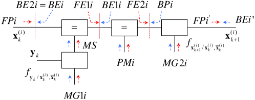
Figure 1: Factor graph involved in the $k-$th ($(T-k)-$th) recursion of Bayesian filtering (BIF) for the substate $\mathbf{x}_{k}^{(i)}$ and forward (backward) message passing on it. The flow of messages in the forward (backward) pass are indicated by red (blue) arrows, respectively; the brown vertical lines cutting each graph identify the partitioning associated with formulas (10) (left cut), (11) (central cut) and (12) (right cut). The messages $\vec{m}_{\mathrm{fp}}(\mathbf{x}_{k}^{(i)})$, $\reflectbox{$\vec{\reflectbox{$m$}}$}_{\mathrm{bp}}(\mathbf{x}_{k}^{(i)})$, $\vec{m}_{\mathrm{fp}}(\mathbf{x}_{k+1}^{(i)})$, $\reflectbox{$\vec{\reflectbox{$m$}}$}_{\mathrm{be}}(\mathbf{x}_{k+1}^{(i)})$, $m_{\mathrm{ms}}(\mathbf{x}_{k}^{(i)})$, $m_{\mathrm{mg}l}(\mathbf{\bar{x}}_{k}^{(i)})$, $m_{\mathrm{pm}}(\mathbf{x}_{k}^{(i)})$, $\vec{m}_{\mathrm{fe}l}(\mathbf{x}_{k}^{(i)})$ and $\reflectbox{$\vec{\reflectbox{$m$}}$}_{\mathrm{be}l}(\mathbf{x}_{k}^{(i)})$ are denoted $FPi$, $BPi$, $FPi^{{}^{\prime}}$, $BEi^{{}^{\prime}}$, $MSi$, $MGli$, $PMi$, $FEli$ and $BEli$ respectively, to ease reading.

Given the graphical model represented in Fig. 1, step 3. can be accomplished by adopting the same conceptual approach as [19, Sec. III] and [20, Par. II-B], where the factor graphs on which smoothing and filtering, respectively, are based are obtained by merging two sub-graphs, each referring to a distinct substate. For this reason, in this case, the graphical model for the whole state $\mathbf{x}_{k}$ is obtained by interconnecting two distinct factor graphs, each structured like the one shown in Fig. 1. In [20, Par. II-B], message passing on the resulting graph is described in detail for the case of Bayesian filtering. In this manuscript, instead, our analysis of message passing concerns BIF and smoothing only. The devised graph and the messages passed on it are shown in Fig. 2. Note that, in developing our graphical model, it has been assumed that the smoothed pdf referring to $\mathbf{x}_{k}^{(i)}$ (and conveyed by the message $m_{\mathrm{sm}}(\mathbf{x}_{k}^{(i)})$) is computed on the basis of Eq. (10), i.e. by merging the messages $\vec{m}_{\mathrm{fp}}(\mathbf{x}_{k}^{(i)})$ and $\reflectbox{$\vec{\reflectbox{$m$}}$}_{\mathrm{be}}(\mathbf{x}_{k}^{(i)})=\reflectbox{$\vec{\reflectbox{$m$}}$}_{\mathrm{be}2}(\mathbf{x}_{k}^{(i)})$. Moreover, the following elements (identified by brown lines) have been added to its $i-$th sub-graph (with $i=1$ and $2$): a) two equality nodes; b) the block BIF${}_{i}{\rightarrow}$BIF_j for extracting useful information from the messages computed on the $i-$th sub-graph and delivered to the $j-$th one. The former elements allow the $i-$th backward information filter to generate copies of the messages $\reflectbox{$\vec{\reflectbox{$m$}}$}_{\mathrm{be}}(\mathbf{x}_{k+1}^{(i)})$ and $m_{\mathrm{sm}}(\mathbf{x}_{k}^{(i)})$, that are made available to the other sub-graphs. In the latter element, instead, the messages $m_{\mathrm{pm}}(\mathbf{x}_{k}^{(i)})$ (see Eq. (3)) and $m_{\mathrm{mg}q}(\mathbf{\bar{x}}_{k}^{(i)})$ (with $q=1$ and $2$; see Eqs. (6) and (7)) are computed; note that this block is connected to oriented edges only, i.e. to edges on which the flow of messages is unidirectional.

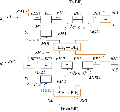
Figure 2: Graphical model based on the sub-graph shown in Fig. 1 and referring to the interconnection of two backward information filters. The message computed in the backward (forward) pass are identified by blue (black) arrows. The message $m_{\mathrm{sm}}(\mathbf{x}_{k}^{(i)})$ is denoted $SMi$ to ease reading.

Given the graphical model represented in Fig. 2, step 4. can be easily accomplished. In fact, recursive BIF and smoothing algorithms can be derived by systematically applying the SPA to it after that a proper scheduling has been established for message passing. In doing so, we must always keep in mind that:
1) Message passing on the $i-$th subgraph represents BIF/smoothing for the substate $\mathbf{x}_{k}^{(i)}$; the exchange of messages between the sub-graphs, instead, allows us to represent the interaction of two interconnected BIF/smoothing algorithms in a effective and rigorous way.
2) Different approximations can be used for the predicted/filtered/smoothed pdfs computed in the message passing on each of the two sub-graphs and for the involved Markov/observation models. For this reason, generally speaking, the two interconnected filtering/BIF/smoothing algorithms are not required to be of the same type.
3) The $k-$th recursion of the overall BIF algorithm is fed by the backward estimates $\reflectbox{$\vec{\reflectbox{$m$}}$}_{\mathrm{be}}(\mathbf{x}_{k+1}^{(1)})$ ($BE1^{\prime}$) and $\reflectbox{$\vec{\reflectbox{$m$}}$}_{\mathrm{be}}(\mathbf{x}_{k+1}^{(2)})$ ($BE2^{\prime}$), and generates the new backward predictions $\reflectbox{$\vec{\reflectbox{$m$}}$}_{\mathrm{bp}}(\mathbf{x}_{k}^{(1)})$ ($BP1$) and $\reflectbox{$\vec{\reflectbox{$m$}}$}_{\mathrm{bp}}(\mathbf{x}_{k}^{(2)})$ ($BP2$), and the two couples of filtered densities $\{(\reflectbox{$\vec{\reflectbox{$m$}}$}_{\mathrm{be}1}(\mathbf{x}_{k}^{(i)})$, $\reflectbox{$\vec{\reflectbox{$m$}}$}_{\mathrm{be}2}(\mathbf{x}_{k}^{(i)}))$, $i=1$, $2\}$ ($\{BE1i$, $BE2i$, $i=1$, $2\}$). Moreover, merging the predicted densities computed in the forward pass (i.e., the messages $\{FPi\}$) with the second backward filtered densities (i.e., the messages $\{BE2i=BEi\}$) allows us to generate the smoothed pdfs for each substate according to Eq. (10). However, a joint filtered/smoothed density for the whole state $\mathbf{x}_{k}$ is unavailable.
4) Specific algorithms are employed to compute the pseudo-measurement and the nuisance substate pdfs in the BIF${}_{i}{\rightarrow}$BIF_j blocks appearing in Fig. 2. These algorithms depend on the considered SSM and on the selected message scheduling; for this reason, a general description of their structure cannot be provided.
5) The graphical model shown in Fig. 2, unlike the one illustrated in Fig. 1, is not cycle free. The presence of cycles raises the problems of identifying all the messages that can be iteratively refined and establishing the order according to which they are computed. Generally speaking, iterative message passing on the devised graphical model involves both the couple of measurement updates and the backward prediction accomplished in each of the interconnected backward information filters. In fact, this should allow each filter to progressively refine the nuisance substate density employed in its second measurement update and backward prediction, and improve the quality of the pseudo-measurements exploited in its first measurement update. For this reason, if $n_{i}$ iterations are run, the overall computational complexity of each recursion is multiplied by $n_{i}$.

The final important issue about the graphical model devised for both Bayesian filtering and BIF concerns the possible presence of redundancy. In all the considerations illustrated above, disjoint substates $\mathbf{x}_{k}^{(1)}$ and $\mathbf{x}_{k}^{(2)}$ have been assumed. Actually, in ref. [20], it has been shown that our graphical approach can be also employed if the substates $\mathbf{x}_{k}^{(1)}$ and $\mathbf{x}_{k}^{(2)}$ cover $\mathbf{x}_{k}$, but do not necessarily form a partition of it. In other words, some overlapping between these two substates is admitted. When this occurs, the forward/backward filtering algorithm run over the whole graphical model contains a form of redundancy, since $N_{d}\triangleq D_{1}+D_{2}-D$ elements of the state vector $\mathbf{x}_{k}$ are independently estimated by the interconnected forward/backward filters. The parameter $N_{d}$ can be considered as the degree of redundancy characterizing the filtering/smoothing algorithm. Moreover, in ref. [20], it has been shown that the presence of redundancy in a Bayesian filtering algorithm can significantly enhance its tracking capability (i.e., reduce its probability of divergence); however, this result is obtained at the price of an increased complexity with respect to the case in which the interconnected filters are run over disjoint substates.

III. Double Backward Information Filtering and Smoothing Algorithms for Conditionally Linear Gaussian State Space Models

In this section we focus on the development of two new DBS algorithms for conditionally linear Gaussian models. We first describe the graphical models on which these algorithms are based; then, we provide a detailed description of the computed messages and their scheduling in a specific case.

A. Graphical Modelling

In this paragraph, we focus on a specific instance of the graphical model illustrated in Fig. 2, since we make the same specific choices as ref. [20] for both the considered SSM and the two Bayesian filters employed in the forward pass. For this reason, we assume that: a) the SSM described by eqs. (1)-(2) is conditionally linear Gaussian [18], [23], [24], so that its state vector $\mathbf{x}_{k}$ can be partitioned into its linear component $\mathbf{x}_{k}^{(L)}$ and its nonlinear component $\mathbf{x}_{k}^{(N)}$ (having sizes $D_{L}$ and $D_{N}$, respectively, with $D_{N}+D_{L}=D$); b) the dual Bayesian filter employed in the forward pass results from the interconnection of an extended Kalman filter with a particle filter (these filters are denoted F₁ and F₂, respectively), as described in detail in ref. [20]. As far as the last point is concerned, it is also worth mentioning that, on the one hand, filter F₂ estimates the nonlinear state component only (so that $\mathbf{x}_{k}^{(2)}=\mathbf{x}_{k}^{(N)}$ and $\mathbf{\bar{x}}_{k}^{(2)}=\mathbf{x}_{k}^{(L)}$) and approximates the predicted/filtered densities of this component through a set of $N_{p}$ weighted particles. On the other hand, filter F₁ employs a Gaussian approximation of all its predicted/filtered densities, and works on the whole system state or on the linear state component. In the first case (denoted C.1 in the following), we have that $\mathbf{x}_{k}^{(1)}=\mathbf{x}_{k}$ and $\mathbf{\bar{x}}_{k}^{(1)}$ is empty, so that both F₁ and F₂ estimate the nonlinear state component (for this reason, the corresponding degree of redundancy in the developed smoothing algorithm is $N_{d}=D_{N}$); in the second case (denoted C.2 in the following), instead, $\mathbf{x}_{k}^{(1)}=\mathbf{x}_{k}^{(L)}$ and $\mathbf{\bar{x}}_{k}^{(1)}=\mathbf{x}_{k}^{(N)}$, so that filters F₁ and F₂ estimate disjoint substates (consequently, $N_{d}=0$).

Our selection of the forward filtering scheme has the following implications on the developed DBIF scheme. The first backward information filter (denoted BIF₁) is the backward filter associated with an extended Kalman filter operating over on the whole system state (case C.1) or on the linear state component (case C.2). The second backward filter (denoted BIF₂), instead, is a backward filter associated with a particle filter operating on the nonlinear state component only. In practice, following [18, 19, 17], BIF₂ is employed to update the weights of all the elements of the particle set generated by filter F₂ in the forward pass. Then, based on the graphical model shown in Fig. 2, the factor graph illustrated in Fig. 3 can be drawn for case C.1. It is important to point out that:

1) The first backward information filter (BIF₁) is based on linearised (and, consequently, approximate) Markov/measurement models, whereas the second one (BIF₂) relies on exact models, as explained in more detail below. These models are the same as those employed in ref. [20].

2) Since the nuisance substate $\mathbf{\bar{x}}_{k}^{(1)}$ is empty, no marginalization is required in BIF₁; for this reason, the messages $\{m_{\mathrm{mg}q}(\mathbf{\bar{x}}_{k}^{(1)})$; $q=1,2\}$ (i.e., $MG11$ and $MG21$) visible in Fig. 2 do not appear in Fig. 3. Moreover, the message $m_{\mathrm{sm}}(\mathbf{x}_{k}^{(1)})=m_{\mathrm{sm}}(\mathbf{x}_{k})$ is generated on the basis of Eq. (11), instead of Eq. (10).

3) The backward filtered pdf $\reflectbox{$\vec{\reflectbox{$m$}}$}_{\mathrm{be}}(\mathbf{x}_{k+1}^{(2)})=\reflectbox{$\vec{\reflectbox{$m$}}$}_{\mathrm{be}}(\mathbf{x}_{k+1}^{(N)})$ and the smoothed pdf $m_{\mathrm{sm}}(\mathbf{x}_{k}^{(2)})=m_{\mathrm{sm}}(\mathbf{x}_{k}^{(N)})$ (i.e., the messages $BE2^{{}^{\prime}}$ and $SM2$, respectively) feed the BIF${}_{2}{\rightarrow}$BIF₁ block, where they are processed jointly to generate the pseudo-measurement message $m_{\mathrm{pm}}(\mathbf{x}_{k}^{(1)})=m_{\mathrm{pm}}(\mathbf{x}_{k})$ ($PM1$) feeding filter F₁. Similarly, the backward filtered pdf $\reflectbox{$\vec{\reflectbox{$m$}}$}_{\mathrm{be}}(\mathbf{x}_{k+1}^{(1)})=\reflectbox{$\vec{\reflectbox{$m$}}$}_{\mathrm{be}}(\mathbf{x}_{k+1})$ ($BE1\prime$) and the smoothed pdf $m_{\mathrm{sm}}(\mathbf{x}_{k}^{(1)})=m_{\mathrm{sm}}(\mathbf{x}_{k})$ ($SM1$) feed the BIF${}_{1}{\rightarrow}$BIF₂ block, where the pseudo-measurement message $m_{\mathrm{pm}}(\mathbf{x}_{k}^{(2)})=m_{\mathrm{pm}}(\mathbf{x}_{k}^{(N)})$ ($PM2$) and the messages $\{m_{\mathrm{mg}q}(\mathbf{\bar{x}}_{k}^{(2)})=m_{\mathrm{mg}q}(\mathbf{x}_{k}^{(L)})$; $q=1,2\}$ (i.e., $MG12$ and $MG22$) are evaluated.

In the remaining part of this paragraph, we first provide various details about the backward filters BIF₁ and BIF₂, and the way pseudo-measurements are computed for each of them; then, we comment on how the factor graph shown in Fig. 3 should be modified if case C.2 is considered.

BIF₁ - This backward filter is based on the linearized versions of Eqs. (1) and (2), i.e. on the models (e.g., see [1, pp. 194-195] and [20, Par. III-A])

$$\mathbf{x}_{k+1}=\mathbf{F}_{k}\,\mathbf{x}_{k}+\mathbf{u}_{k}+\mathbf{w}_{k}$$ (13)

and

$$\mathbf{y}_{k}=\mathbf{H}_{k}^{T}\,\mathbf{x}_{k}+\mathbf{v}_{k}+\mathbf{e}_{k},$$ (14)

respectively; here, $\mathbf{F}_{k}\triangleq[\partial\mathbf{f}_{k}\left(\mathbf{x}\right)/\partial\mathbf{x}]_{\mathbf{x=x}_{\mathrm{fe},k}}$, $\mathbf{u}_{k}\triangleq\mathbf{f}_{k}\left(\mathbf{x}_{\mathrm{fe},k}\right)-\mathbf{F}_{k}\,\mathbf{x}_{\mathrm{fe},k}$, $\mathbf{H}_{k}^{T}\triangleq[\partial\mathbf{h}_{k}\left(\mathbf{x}\right)/\partial\mathbf{x}]_{\mathbf{x=x}_{\mathrm{fp},k}}$, $\mathbf{v}_{k}\triangleq\mathbf{h}_{k}\left(\mathbf{x}_{\mathrm{fp},k}\right)-\mathbf{H}_{k}^{T}\mathbf{x}_{\mathrm{fp},k}$ and $\mathbf{x}_{\mathrm{fp},k}$ ($\mathbf{x}_{\mathrm{fe},k}$) is the forward prediction (forward estimate) of $\mathbf{x}_{k}$ computed by F₁ in its $(k-1)-$th ($k-$th) recursion. Consequently, the approximate models

$$\tilde{f}\left(\mathbf{x}_{k+1}\left|\mathbf{x}_{k}\right.\right)=\mathcal{N}\left(\mathbf{x}_{k};\mathbf{F}_{k}\,\mathbf{x}_{k}+\mathbf{u}_{k},\mathbf{C}_{w}\right)$$ (15)

and

$$\tilde{f}\left(\mathbf{y}_{k}\left|\mathbf{x}_{k}\right.\right)=\mathcal{N}\left(\mathbf{x}_{k};\mathbf{H}_{k}^{T}\,\mathbf{x}_{k}+\mathbf{v}_{k},\mathbf{C}_{e}\right)$$ (16)

appear in the graphical model shown in Fig. 3.

BIF₂ - In developing this backward filter, the state vector $\mathbf{x}_{k}$ is represented as the ordered concatenation of its linear component $\mathbf{x}_{k}^{(L)}\triangleq[x_{0,k}^{(L)}$, $x_{1,k}^{(L)},...,x_{D_{L}-1,k}^{(L)}]^{T}$ and its nonlinear component $\mathbf{x}_{k}^{(N)}\triangleq[x_{0,k}^{(N)},x_{1,k}^{(N)},...,x_{D_{N}-1,k}^{(N)}]^{T}$. Based on [23, eq. (3)], the Markov model

$$\mathbf{x}_{k+1}^{(N)}=\mathbf{A}_{k}^{(N)}\left(\mathbf{x}_{k}^{(N)}\right)\mathbf{x}_{k}^{(L)}+\mathbf{f}_{k}^{(N)}\left(\mathbf{x}_{k}^{(N)}\right)+\mathbf{w}_{k}^{(N)}$$ (17)

is adopted for the nonlinear state component (this model corresponds to the last $D_{N}$ lines of Eq. (1)); here, $\mathbf{f}_{k}^{(N)}(\mathbf{x}_{k}^{(N)})$ ($\mathbf{A}_{k}^{(N)}(\mathbf{x}_{k}^{(N)})$) is a time-varying $D_{N}-$dimensional real function ($D_{N}\times D_{L}$ real matrix) and $\mathbf{w}_{k}^{(N)}$ consists of the last $D_{N}$ elements of the noise term $\mathbf{w}_{k}$ appearing in Eq. (1) (the covariance matrix of $\mathbf{w}_{k}^{(N)}$ is denoted $\mathbf{C}_{w}^{(N)}$). Moreover, it is assumed that the observation model (2) can be put in the form (see [20, eq. (31)] or [23, eq. (4)])

$$\mathbf{y}_{k}=\mathbf{g}_{k}\left(\mathbf{x}_{k}^{(N)}\right)+\mathbf{B}_{k}\left(\mathbf{x}_{k}^{(N)}\right)\mathbf{x}_{k}^{(L)}+\mathbf{e}_{k},$$ (18)

where $\mathbf{g}_{k}(\mathbf{x}_{k}^{(N)})$ ($\mathbf{B}_{k}(\mathbf{x}_{k}^{(N)})$) is a time-varying $P-$dimensional real function ($P\times D_{L}$ real matrix). Consequently, the considered backward filter is based on the exact pdfs

$$f\left(\mathbf{x}_{k+1}^{(N)}\left|\mathbf{x}_{k}^{(N)},\mathbf{x}_{k}^{(L)}\right.\right)$$

$$= \mathcal{N}\left(\mathbf{x}_{k}^{(N)};\mathbf{A}_{k}^{(N)}\left(\mathbf{x}_{k}^{(N)}\right)\mathbf{x}_{k}^{(L)}+\mathbf{f}_{k}^{(N)}\left(\mathbf{x}_{k}^{(N)}\right),\mathbf{C}_{w}^{(N)}\right)$$

and

$$f\left(\mathbf{y}_{k}\left|\mathbf{x}_{k}^{(N)},\mathbf{x}_{k}^{(L)}\right.\right)$$ (20)

$$= \mathcal{N}\left(\mathbf{x}_{k};\mathbf{g}_{k}\left(\mathbf{x}_{k}^{(N)}\right)+\mathbf{B}_{k}\left(\mathbf{x}_{k}^{(N)}\right)\mathbf{x}_{k}^{(L)},\mathbf{C}_{e}\right),$$

both appearing in the graphical model drawn in Fig. 3.

Computation of the pseudo-measurements for the first backward filter - Filter BIF₁ is fed by pseudo-measurement information about the whole state $\mathbf{x}_{k}$. The method for computing these information is similar to the one illustrated in ref. [19, Sects. III-IV] and can be summarised as follows. The pseudo-measurements about the nonlinear state component are represented by the $N_{p}$ particles conveyed by the smoothed pdf $m_{\mathrm{sm}}(\mathbf{x}_{k}^{(N)})$ ($SM2$). On the other hand, $N_{p}$ pseudo-measurements about the linear state component are evaluated by means of the same method employed by marginalized particle filtering (MPF) for this task. This method is based on the idea that the random vector (see Eq. (17))

$$\mathbf{z}_{k}^{(L)}\triangleq\mathbf{x}_{k+1}^{(N)}-\mathbf{f}_{k}^{(N)}\left(\mathbf{x}_{k}^{(N)}\right),$$ (21)

depending on the nonlinear state component only, must equal the sum

$$\mathbf{A}_{k}^{(N)}\left(\mathbf{x}_{k}^{(N)}\right)\mathbf{x}_{k}^{(L)}+\mathbf{w}_{k}^{(N)},$$ (22)

that depends on the linear state component. For this reason, $N_{p}$ realizations of $\mathbf{z}_{k}^{(L)}$ (21) are computed in the BIF${}_{2}{\rightarrow}$BIF₁ block on the basis of the messages $\reflectbox{$\vec{\reflectbox{$m$}}$}_{\mathrm{be}}(\mathbf{x}_{k+1}^{(N)})$ ($BE2^{{}^{\prime}}$) and $m_{\mathrm{sm}}(\mathbf{x}_{k}^{(N)})$, and are treated as measurements about $\mathbf{x}_{k}^{(L)}$.

Computation of the pseudo-measurements for the second backward filter - The messages $\reflectbox{$\vec{\reflectbox{$m$}}$}_{\mathrm{be}}(\mathbf{x}_{k+1})$ ($BE1^{\prime}$) and $m_{\mathrm{sm}}(\mathbf{x}_{k})$ ($SM1$) feeding the BIF${}_{1}{\rightarrow}$BIF₂ block are employed for: a) generating the messages $\{m_{\mathrm{mg}q}(\mathbf{x}_{k}^{(L)})$; $q=1,2\}$ required to integrate out the dependence of the state update and measurement models (i.e., of the densities $f(\mathbf{x}_{k+1}^{(N)}|\mathbf{x}_{k}^{(N)}$, $\mathbf{x}_{k}^{(L)})$ (LABEL:f_x_N) and $f(\mathbf{y}_{k}|\mathbf{x}_{k}^{(N)},\mathbf{x}_{k}^{(L)})$ (20), respectively) on the substate $\mathbf{x}_{k}^{(L)}$; b) generating pseudo-measurement information about $\mathbf{x}_{k}^{(N)}$. As far as the last point is concerned, the approach we adopt is the same as that developed for dual marginalized particle filtering (dual MPF) in ref. [23, Sec. V] and also adopted in particle smoothing [19, Sects. III-IV]. The approach relies on the Markov model

$$\mathbf{x}_{k+1}^{(L)}=\mathbf{A}_{k}^{(L)}\left(\mathbf{x}_{k}^{(N)}\right)\mathbf{x}_{k}^{(L)}+\mathbf{f}_{k}^{(L)}\left(\mathbf{x}_{k}^{(N)}\right)+\mathbf{w}_{k}^{(L)},$$ (23)

referring to the linear state component (see [19, eq. (1)] or [23, eq. (3)]); in the last expression, $\mathbf{f}_{k}^{(L)}(\mathbf{x}_{k}^{(N)})$ ($\mathbf{A}_{k}^{(L)}(\mathbf{x}_{k}^{(N)})$) is a time-varying $D_{L}-$dimensional real function ($D_{L}\times D_{L}$ real matrix), and $\mathbf{w}_{k}^{(L)}$ consists of the first $D_{L}$ elements of the noise term $\mathbf{w}_{k}$ appearing in (1) (the covariance matrix of $\mathbf{w}_{k}^{(L)}$ is denoted $\mathbf{C}_{w}^{(L)}$, and independence between $\{\mathbf{w}_{k}^{(L)}\}$ and $\{\mathbf{w}_{k}^{(N)}\}$ is assumed for simplicity). From Eq. (23) it is easily inferred that the random vector

$$\mathbf{z}_{k}^{(N)}\triangleq\mathbf{x}_{k+1}^{(L)}-\mathbf{A}_{k}^{(L)}\left(\mathbf{x}_{k}^{(N)}\right)\,\mathbf{x}_{k}^{(L)}\text{,}$$ (24)

must equal the sum

$$\mathbf{f}_{k}^{(L)}\left(\mathbf{x}_{k}^{(N)}\right)+\mathbf{w}_{k}^{(L)},$$ (25)

that depends on $\mathbf{x}_{k}^{(N)}$ only; for this reason, $\mathbf{z}_{k}^{(N)}$ (24) can be interpreted as a pseudo-measurement about $\mathbf{x}_{k}^{(N)}$. In this case, the pseudo-measurement information is conveyed by the message $m_{\mathrm{pm}}(\mathbf{x}_{k}^{(N)})$ ($PM2$) that expresses the correlation between the pdf of the random vector $\mathbf{z}_{k}^{(N)}$ (24) (computed on the basis of the statistical information about the linear state component made available by BIF₁) and the pdf obtained for $\mathbf{z}_{k}^{(N)}$ under the assumption that this vector is expressed by Eq. (25). The message $m_{\mathrm{pm}}(\mathbf{x}_{k}^{(N)})$ is evaluated for each of the particles representing $\mathbf{x}_{k}^{(N)}$ in BIF₂; this results in a set of $N_{p}$ particle weights employed in the first measurement update of BIF₂ and different from those computed on the basis of $\mathbf{y}_{k}$ (18) in its second measurement update.

A graphical model similar to the one shown in Fig. 3 can be easily derived from the general model appearing in Fig. 2 for case C.2 too. The relevant differences with respect to case C.1 can be summarized as follows:

1) The backward filters BIF₁ and BIF₂ estimate $\mathbf{x}_{k}^{(1)}=\mathbf{x}_{k}^{(L)}$ and $\mathbf{x}_{k}^{(2)}=\mathbf{x}_{k}^{(N)}$, respectively; consequently, their nuisance substates are $\mathbf{\bar{x}}_{k}^{(1)}=\mathbf{x}_{k}^{(N)}$ and $\mathbf{\bar{x}}_{k}^{(2)}=\mathbf{x}_{k}^{(L)}$, respectively.

2) The BIF${}_{2}{\rightarrow}$BIF₁ block is fed by the backward predicted/smoothed pdfs computed by BIF₂; such pdfs are employed for: a) generating the messages $m_{\mathrm{mg}1}(\mathbf{x}_{k}^{(N)})$ ($MG11$) and $m_{\mathrm{mg}2}(\mathbf{x}_{k}^{(N)})$ ($MG21$) required to integrate out the dependence of the Markov model (see Eq. (23))

$$f\left(\mathbf{x}_{k+1}^{(L)}\left|\mathbf{x}_{k}^{(N)},\mathbf{x}_{k}^{(L)}\right.\right)$$

$$= \mathcal{N}\left(\mathbf{x}_{k}^{(L)};\mathbf{A}_{k}^{(L)}\left(\mathbf{x}_{k}^{(N)}\right)\mathbf{x}_{k}^{(L)}+\mathbf{f}_{k}^{(L)}\left(\mathbf{x}_{k}^{(N)}\right),\mathbf{C}_{w}^{(L)}\right)$$

and of the measurement model $f(\mathbf{y}_{k}|\mathbf{x}_{k}^{(N)},\mathbf{x}_{k}^{(L)})$ (20), respectively, on $\mathbf{x}_{k}^{(N)}$; b) generating pseudo-measurement information about the substate $\mathbf{x}_{k}^{(L)}$ only. As far as point a) is concerned, it is also important to point out that the model $f(\mathbf{y}_{k}|\mathbf{x}_{k}^{(N)},\mathbf{x}_{k}^{(L)})$ ($f(\mathbf{x}_{k+1}^{(L)}|\mathbf{x}_{k}^{(N)},\mathbf{x}_{k}^{(L)})$) on which BIF₁ is based can be derived from Eq. (20) (Eq. (LABEL:f_x_L)) after setting $\mathbf{x}_{k}^{(N)}=\mathbf{x}_{\mathrm{fp},k}^{(N)}$ ($\mathbf{x}_{k}^{(N)}=\mathbf{x}_{\mathrm{fe},k}^{(N)}$); here, $\mathbf{x}_{\mathrm{fp},k}^{(N)}$ ($\mathbf{x}_{\mathrm{fe},k}^{(N)}$) denotes the prediction (the estimate) of $\mathbf{x}_{k}^{(N)}$ evaluated by the filter F₂ in the forward pass (further details about this can be found in ref. [20, Par. III-A])

The derivation of specific DBS algorithms based on the graphical model illustrated in Fig. 3 requires defining the scheduling of the messages passed on it and deriving mathematical expressions for such messages. These issues are investigated in detail in the following paragraph.

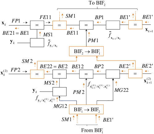
Figure 3: Graphical model referring to the interconnection of two backward information filters, one paired with an extended Kalman filter, the other one with a particle filter.

B. Message Scheduling and Computation

In this paragraph, the scheduling of a new recursive smoothing algorithm, called double Bayesian smoothing algorithm (DBSA) and based on the graphical model illustrated in Fig. 3, and a simplified version of it are described. Moreover, the expression of the messages computed by the DBSA are illustrated.

The scheduling adopted in the DBSA mimics the one employed in ref. [19] (which, in turn, has been inspired by [17] and [18]). Moreover, in devising it, the presence of cycles in the underlying graphical model has been accounted for by allowing multiple passes of messages over the edges which such cycles consist of; this explains why an iterative procedure is embedded in each recursion of the DBSA. Our description of the devised scheduling is based on Fig. 4, that refers to the $(T-k)-$th recursion of the backward pass of the DBSA (with $k=T-1$, $T-2$, $...$, $1$) and to the $n-$th iteration accomplished within this recursion (with $n=1$, $2$, $...$, $n_{i}$, where $n_{i}$ represents the overall number of iterations). Note that, in this figure, a simpler notation is adopted for most of the considered messages to ease reading; in particular, the symbols $q$ , $q^{(n)}$, $qL$, $qL^{(n)}$, $qN$ and $qN^{(n)}$ are employed to represent the messages $m_{q}(\mathbf{x}_{k})$, $m_{q}^{(n)}(\mathbf{x}_{k})$, $m_{q}(\mathbf{x}_{k}^{(L)})$, $m_{q}^{(n)}(\mathbf{x}_{k}^{(L)})$, $m_{q}(\mathbf{x}_{k}^{(N)})$, $m_{q}^{(n)}(\mathbf{x}_{k}^{(N)})$, respectively (independently of the presence of an arrow and of its direction in the considered message), and the presence of the superscript $(n)$ in a given message means that such a message is computed in the $n$-th iteration. Moreover, each of the passed messages conveys a Gaussian pdf or a pdf in particle form. In the first case, the pdf of a state/substate $\mathbf{x}$ is conveyed by the message

$$m_{G}\left(\mathbf{x}\right)=\mathcal{N(}\mathbf{x};\mathbf{\eta},\mathbf{C}),$$ (27)

where $\mathbf{\eta}$ and $\mathbf{C}$ denote the mean and the covariance of $\mathbf{x}$, respectively. In the second case, instead, its pdf is conveyed by the message

$$m_{P}\left(\mathbf{x}\right)=\sum_{j=1}^{N_{p}}{m}_{P,j}\left(\mathbf{x}\right),$$ (28)

where

$$m_{P,j}\left(\mathbf{x}\right)\triangleq w_{j}\,\delta\left(\mathbf{x}-\mathbf{x}_{j}\right)$$ (29)

is its $j-$th component; this represents the contribution of the $j-$th particle $\mathbf{x}_{j}$ and its weight $w_{j}$ to ${m}_{P}(\mathbf{x})$ (28). The nature of each message can be easily inferred from Fig. 4, since Gaussian messages and messages in particle form are identified by blue and red arrows, respectively.

Before analysing the adopted scheduling, we need to define the input messages feeding the considered recursion of the DBSA and the outputs that such a recursion produces. In the considered recursion, the DBSA input messages originate from:

1) The $k$-th recursion of the forward pass. These messages have been generated by the DBF technique paired with the considered BIF scheme and, in particular, by the DBF algorithm derived in ref. [20, Par. III-B], and have been stored (so that they are made available to the backward pass).

2) The previous recursion (i.e., the $(T-k-1)-$th recursion) of the DBSA itself.

As far as the input messages computed in the forward pass are concerned, BIF₁ is fed by the Gaussian messages (see Fig. 4)

$$\vec{m}_{\mathrm{fp}}\left(\mathbf{x}_{k}\right)\triangleq\mathcal{N}\left(\mathbf{x}_{k};\mathbf{\eta}_{\mathrm{fp},k},\mathbf{C}_{\mathrm{fp},k}\right).$$ (30)

and

$$\vec{m}_{\mathrm{fe}1}\left(\mathbf{x}_{k}\right)\triangleq\mathcal{N}\left(\mathbf{x}_{k};\mathbf{\eta}_{\mathrm{fe}1,k},\mathbf{C}_{\mathrm{fe}1,k}\right),$$ (31)

that convey the predicted pdf and the first filtered pdf, respectively, computed by F₁ (in its $(k-1)-$th and in its $k-$th recursion, respectively). The covariance matrix $\mathbf{C}_{\mathrm{fe}1,k}$ and the mean vector $\mathbf{\eta}_{\mathrm{fe}1,k}$ are evaluated on the basis of the associated precision matrix (see [19, Eqs. (14)-(17)])

$$\mathbf{W}_{\mathrm{fe}1,k}=\mathbf{H}_{k}\,\mathbf{W}_{e}\,\mathbf{H}_{k}^{T}+\mathbf{W}_{\mathrm{fp},k}$$ (32)

and of the associated transformed mean vector

$$\mathbf{w}_{\mathrm{fe}1,k}=\mathbf{H}_{k}\,\mathbf{W}_{e}\left(\mathbf{y}_{k}-\mathbf{v}_{k}\right)+\mathbf{w}_{\mathrm{fp},k},$$ (33)

respectively; here, $\mathbf{W}_{e}\triangleq\mathbf{C}_{e}^{-1}$, $\mathbf{W}_{\mathrm{fp},k}\triangleq(\mathbf{C}_{\mathrm{fp},k})^{-1}$ and $\mathbf{w}_{\mathrm{fp},k}\triangleq\mathbf{W}_{\mathrm{fp},k}\,\mathbf{\eta}_{\mathrm{fp},k}$.

The backward filter BIF₂, instead, is fed by the forward messages $\vec{m}_{\mathrm{fp}}(\mathbf{x}_{k}^{(N)})$ and $\vec{m}_{\mathrm{fe}1}(\mathbf{x}_{k}^{(N)})$, both in particle form (see Fig. 4); their $j-$th components are represented by

$$\vec{m}_{\mathrm{fp},j}\left(\mathbf{x}_{k}^{(N)}\right)\triangleq w_{p}\,\delta\left(\mathbf{x}_{k}^{(N)}-\mathbf{x}_{k,j}^{(N)}\right),$$ (34)

and

$$\vec{m}_{\mathrm{fe}1,j}\left(\mathbf{x}_{k}^{(N)}\right)\triangleq w_{\mathrm{fe},k,j}\,\delta\left(\mathbf{x}_{k}^{(N)}-\mathbf{x}_{k,j}^{(N)}\right),$$ (35)

respectively, with $j=1,2,...,N_{p}$; here, $\mathbf{x}_{k,j}^{(N)}$ is the $j-$th particle predicted by F₂ in the $(k-1)$-th recursion of the forward pass (i.e., the $j-$th element of the particle set $S_{k}\triangleq\{\mathbf{x}_{k,1}^{(N)}$, $\mathbf{x}_{k,2}^{(N)}$, $...$, $\mathbf{x}_{k,N_{p}}^{(N)}\}$), whereas $w_{p}\triangleq 1/N_{p}$ and $w_{\mathrm{fe},k,j}$ represent the (normalised) weights assigned to this particle in the messages $\vec{m}_{\mathrm{fp}}(\mathbf{x}_{k}^{(N)})$ and $\vec{m}_{\mathrm{fe}1}(\mathbf{x}_{k}^{(N)})$, respectively.

On the other hand, the input messages originating from the previous recursion of the backward pass are the backward filtered Gaussian pdf

$$\reflectbox{$\vec{\reflectbox{$m$}}$}_{\mathrm{be}}\left(\mathbf{x}_{k+1}\right)\triangleq\mathcal{N}\left(\mathbf{x}_{k+1};\mathbf{\eta}_{\mathrm{be},k+1},\mathbf{C}_{\mathrm{be},k+1}\right)$$ (36)

and the backward pdf

$$\reflectbox{$\vec{\reflectbox{$m$}}$}_{\mathrm{be}}\left(\mathbf{x}_{k+1}^{(N)}\right)\triangleq\delta\left(\mathbf{x}_{k+1}^{(N)}-\mathbf{x}_{\mathrm{be},k+1}^{(N)}\right),$$ (37)

that represents $\mathbf{x}_{k+1}^{(N)}$ through a single particle having unit weight; these are computed by BIF₁ and BIF₂, respectively. Consequently, in the considered recursion of the backward pass, all the forward/backward input messages described above are processed to compute: 1) the new backward pdfs $\reflectbox{$\vec{\reflectbox{$m$}}$}_{\mathrm{be}}(\mathbf{x}_{k})$ and $\reflectbox{$\vec{\reflectbox{$m$}}$}_{\mathrm{be}}(\mathbf{x}_{k}^{(N)})$; 2) the smoothed statistical information about $\mathbf{x}_{k}$ ($\mathbf{x}_{k}^{(N)}$) by properly merging forward and backward messages generated by F₁ and BIF₁ (F₂ and BIF₂). As far as the last point is concerned, the evaluation of smoothed information is based on the same conceptual approach as [17, 18, 19]. In fact, in our work, the joint smoothing pdf $f(\mathbf{x}_{1:T}|\mathbf{y}_{1:T})$ is estimated by providing multiple (say, $M$) realizations of it. A single realization (i.e., a single smoothed state trajectory) is computed in each backward pass; consequently, generating the whole output of the DBSA requires running a single forward pass and $M$ distinct backward passes. Moreover, the evaluation of the smoothed information is based on the factorisation (10) or (11). In fact, these formulas are exploited to merge the statistical information emerging from the forward pass with that computed in any of the $M$ backward passes.

The message passing on which the DBSA is based can be divided in the three consecutive phases listed below.

Phase I - In the first phase, the backward predicted pdf $\reflectbox{$\vec{\reflectbox{$m$}}$}_{1}(\mathbf{x}_{k})$ ($1$) is computed on the basis of the backward filtered pdf $\reflectbox{$\vec{\reflectbox{$m$}}$}_{\mathrm{be}}(\mathbf{x}_{k+1})$ ($BE1^{\prime}$).

Phase II - In this phase, an iterative procedure for computing and progressively refining the first backward filtered and the smoothed pdfs of the whole state (BIF₁), and the second filtered and the smoothed pdfs of the nonlinear state component (BIF₂) is carried out. More specifically, in the $n$-th iteration of this procedure (with $n=1$, $2$, $...$, $n_{i}$), the ordered computation of the following messages is accomplished in eight consecutive steps (see Fig. 4): 1) $m_{2}^{(n)}(\mathbf{x}_{k})$ ($2^{(n)}$; pdf conveying pseudo-measurement information about $\mathbf{x}_{k}$); 2) $\reflectbox{$\vec{\reflectbox{$m$}}$}_{3}^{(n)}(\mathbf{x}_{k})$ ($3^{(n)}$; first backward filtered pdf of $\mathbf{x}_{k}$); 3) $m_{4}^{(n)}(\mathbf{x}_{k})$ ($4^{(n)}$; smoothed pdf of $\mathbf{x}_{k}$); 4) $m_{1}^{(n)}(\mathbf{x}_{k}^{(L)})$ ($1L^{(n)}$; pdf for integrating out the dependence of $f(\mathbf{x}_{k+1}^{(N)}|\mathbf{x}_{k}^{(N)},\mathbf{x}_{k}^{(L)})$ and $f(\mathbf{y}_{k}|\mathbf{x}_{k}^{(N)},\mathbf{x}_{k}^{(L)})$ on $\mathbf{x}_{k}^{(L)}$), $\reflectbox{$\vec{\reflectbox{$m$}}$}_{3}^{(n)}(\mathbf{x}_{k}^{(N)})$ ($3N^{(n)}$; backward predicted pdf of $\mathbf{x}_{k}^{(N)}$); 5) $m_{2}^{(n)}(\mathbf{x}_{k}^{(N)})$ ($2N^{(n)}$; pdf conveying pseudo-measurement information about $\mathbf{x}_{k}^{(N)}$); 6) $m_{4}^{(n)}(\mathbf{x}_{k}^{(N)})$ ($4N^{(n)}$; first backward filtered pdf of $\mathbf{x}_{k}^{(N)}$); 7) $m_{5}^{(n)}(\mathbf{x}_{k}^{(N)})$ ($5N^{(n)}$; message conveying measurement-based information about $\mathbf{x}_{k}^{(N)}$); 8) $m_{6}^{(n)}(\mathbf{x}_{k}^{(N)})$ ($6N^{(n)}$; second backward filtered pdf of $\mathbf{x}_{k}^{(N)}$), $m_{1}^{(n)}(\mathbf{x}_{k}^{(N)})$ ($1N^{(n)}$; smoothed pdf of $\mathbf{x}_{k}^{(N)}$). Note that the message $m_{1}^{(n)}(\mathbf{x}_{k}^{(N)})$ computed in the last step of the $n$-th iteration is stored in a memory cell (identified by the label ‘D’), so that it becomes available at the beginning of the next iteration.

Phase III - In the third phase, the final smoothed pdf $m_{1}^{(n_{i})}(\mathbf{x}_{k}^{(N)})$ is exploited to compute: a) the final backward pdf (i.e., the output message of BIF₂) $\reflectbox{$\vec{\reflectbox{$m$}}$}_{\mathrm{be}}(\mathbf{x}_{k}^{(N)})$; b) the new pseudo-measurement message $m_{2}^{(n_{i}+1)}(\mathbf{x}_{k})$, the final backward filtered pdf $\reflectbox{$\vec{\reflectbox{$m$}}$}_{3}^{(n_{i}+1)}(\mathbf{x}_{k})$, the final smoothed pdf $m_{4}^{(n_{i}+1)}(\mathbf{x}_{k})$ of $\mathbf{x}_{k}$ and, finally, the final backward pdf (i.e., the output message of BIF₁) $m_{\mathrm{be}}(\mathbf{x}_{k})$.

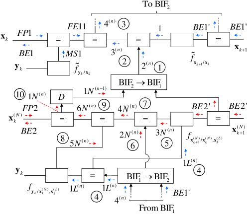
Figure 4: Representation of the message scheduling accomplished within the $(T-k)-$th recursion of the backward pass of the DBSA; the circled integers $1-10$ specify the order according to which the passed messages are computed in the $n-$th iteration embedded in the considered recursion. Blue and red arrows are employed to identify Gaussian messages and messages in particle form, respectively.

C. Message Computation

The expressions of all the messages evaluated by the DBSA, with the exception of the messages emerging from the BIF${}_{1}{\rightarrow}$BIF₂ block and the BIF${}_{2}{\rightarrow}$BIF₁ block, can be easily derived by applying the few mathematical rules listed in Tables I-III of ref. [23, App. A]; all such rules result from the application of the SPA to equality nodes or nodes representing Gaussian functions. The derivation of the algorithms for computing the pseudo-measurement messages $m_{2}^{(n)}(\mathbf{x}_{k})$ ($2^{(n)}$) and $m_{2}^{(n)}(\mathbf{x}_{k}^{(N)})$ ($2N^{(n)}$) emerging from the BIF${}_{2}{\rightarrow}$BIF₁ block and the BIF${}_{1}{\rightarrow}$BIF₂ block, respectively, is based on the same approach illustrated in refs. [19, Par. IV-B] and [23, Sects. IV-V]. On the other hand, the message $m_{1}^{(n)}(\mathbf{x}_{k}^{(L)})$ ($1L^{(n)}$) originating from the BIF${}_{1}{\rightarrow}$BIF₂ block results from marginalizing $m_{4}^{(n)}(\mathbf{x}_{k})$ ($4^{(n)}$) with respect to $\mathbf{x}_{k}^{(N)}$.

In the remaining part of this paragraph, the expressions of all the messages computed in each of the three phases described above are provided for the ($T-k)-$th recursion of the backward pass; the derivation of these expressions is sketched in Appendix A.

Phase I - The computation of the backward predicted pdf

$$\reflectbox{$\vec{\reflectbox{$m$}}$}_{1}\left(\mathbf{x}_{k}\right)\triangleq\mathcal{N}\left(\mathbf{x}_{k};\mathbf{\eta}_{1,k},\mathbf{C}_{1,k}\right)$$ (38)

of $\mathbf{x}_{k}$ involves $\reflectbox{$\vec{\reflectbox{$m$}}$}_{\mathrm{be}}(\mathbf{x}_{k+1})$ (36) and the pdf $\tilde{f}(\mathbf{x}_{k+1}|\mathbf{x}_{k})$ (15). Its parameters $\mathbf{\eta}_{1,k}$ and $\mathbf{C}_{1,k}$ are evaluated on the basis of the associated precision matrix

$$\mathbf{W}_{1,k}\triangleq\left(\mathbf{C}_{1,k}\right)^{-1}=\mathbf{F}_{k}^{T}\,\mathbf{P}_{k+1}\,\mathbf{W}_{\mathrm{be},k+1}\mathbf{F}_{k}$$ (39)

and of the associated transformed mean vector

$$\mathbf{w}_{1,k} \triangleq \mathbf{W}_{1,k}\mathbf{\eta}_{1,k}=\mathbf{F}_{k}^{T}[\mathbf{P}_{k+1}\,\mathbf{w}_{\mathrm{be},k+1}-\mathbf{W}_{\mathrm{be},k+1}\,\mathbf{Q}_{k+1}\,\mathbf{W}_{w}\,\mathbf{u}_{k}],$$

respectively; here, $\mathbf{W}_{\mathrm{be},k+1}\triangleq(\mathbf{C}_{\mathrm{be},k+1})^{-1}$, $\mathbf{P}_{k+1}\triangleq\mathbf{\mathbf{I}}_{D}-\mathbf{W}_{\mathrm{be},k+1}\,\mathbf{Q}_{k+1}$, $\mathbf{Q}_{k+1}\triangleq(\mathbf{W}_{w}+\mathbf{W}_{\mathrm{be},k+1})^{-1}$, $\mathbf{W}_{w}\triangleq(\mathbf{C}_{w})^{-1}$ and $\mathbf{w}_{\mathrm{be},k+1}\triangleq\mathbf{W}_{\mathrm{be},k+1}\,\mathbf{\eta}_{\mathrm{be},k+1}$.

Phase II - In the $n-$th iteration of this phase, the eight consecutive steps listed below are carried out; for each step, all the computed messages are described.

Step 1) - In this step, the message

$$m_{1}^{(n-1)}\left(\mathbf{x}_{k}^{(N)}\right)=\sum_{j=1}^{N_{p}}W_{1,k,j}^{(n-1)}\,\delta\left(\mathbf{x}_{k}^{(N)}-\mathbf{x}_{k,j}^{(N)}\right),$$ (41)

computed in the previous iteration and conveying the smoothed pdf of $\mathbf{x}_{k}^{(N)}$ generated by F₂ and BIF₂ (see step 8)) is processed jointly with $\reflectbox{$\vec{\reflectbox{$m$}}$}_{\mathrm{be}}(\mathbf{x}_{k+1}^{(N)})$ (37) in the BIF${}_{2}{\rightarrow}$BIF₁ block to generate the message

$$m_{2}^{(n)}\left(\mathbf{x}_{k}\right)=\mathcal{\mathcal{N}}\left(\mathbf{x}_{k};\mathbf{\eta}_{2,k}^{(n)},\mathbf{C}_{2,k}^{(n)}\right),$$ (42)

that conveys the pseudo-measurement information provided to BIF₁. The mean vector $\mathbf{\eta}_{2,k}^{(n)}$ and the covariance matrix $\mathbf{C}_{2,k}^{(n)}$ are evaluated as

$$\mathbf{\eta}_{2,k}^{(n)}=\left[\left(\mathbf{\eta}_{L,k}^{(n)}\right)^{T},\left(\mathbf{\eta}_{N,k}^{(n)}\right)^{T}\right]^{T}$$ (43)

and

$$\mathbf{C}_{2,k}^{(n)}=\left[\begin{array}[]{cc}\mathbf{C}_{LL,k}^{(n)}&\mathbf{C}_{LN,k}^{(n)}\\ \left(\mathbf{C}_{LN,k}^{(n)}\right)^{T}&\mathbf{C}_{NN,k}^{(n)}\end{array}\right],$$ (44)

respectively, where

$$\mathbf{\eta}_{X,k}^{(n)}\triangleq\sum_{j=1}^{N_{p}}W_{1,k,j}^{(n-1)}\,\mathbf{\eta}_{X,k,j}$$ (45)

is a $D_{X}$-dimensional mean vector (with $X=L$ and $N)$,

$$\mathbf{C}_{XY,k}^{(n)}\triangleq\sum_{j=1}^{N_{p}}W_{1,k,j}^{(n-1)}\,\mathbf{r}_{XY,k,j}-\mathbf{\eta}_{X,k}\left(\mathbf{\eta}_{Y,k}\right)^{T}$$ (46)

is a $D_{X}\times D_{Y}$ covariance (or cross-covariance) matrix (with $XY=LL$, $NN$ and $LN)$, $\mathbf{\eta}_{L,k,j}=\mathbf{\tilde{\eta}}_{k,j}$, $\mathbf{\eta}_{N,k,j}=\mathbf{x}_{k,j}^{(N)}$, $\mathbf{r}_{LL,k,j}\triangleq\mathbf{\tilde{C}}_{k,j}+\mathbf{\tilde{\eta}}_{k,j}(\mathbf{\tilde{\eta}}_{k,j})^{T}$, $\mathbf{r}_{NN,k,j}\triangleq\mathbf{x}_{k,j}^{(N)}(\mathbf{x}_{k,j}^{(N)})^{T}$ and $\mathbf{r}_{LN,k,j}\triangleq\mathbf{\tilde{\eta}}_{k,j}(\mathbf{x}_{k,j}^{(N)})^{T}$. The covariance matrix $\mathbf{\tilde{C}}_{k,j}$ and the mean vector $\mathbf{\tilde{\eta}}_{k,j}$ are computed on the basis of the associated precision matrix

$$\mathbf{\tilde{W}}_{k,j}\triangleq\left(\mathbf{\tilde{C}}_{k,j}\right)^{-1}=\left(\mathbf{A}_{k,j}^{(N)}\right)^{T}\mathbf{W}_{w}^{(N)}\mathbf{A}_{k,j}^{(N)}$$ (47)

and of the associated transformed mean vector

$$\mathbf{\tilde{w}}_{k,j}\triangleq\mathbf{\tilde{W}}_{k,j}\mathbf{\tilde{\eta}}_{k,j}=\left(\mathbf{A}_{k,j}^{(N)}\right)^{T}\mathbf{W}_{w}^{(N)}\mathbf{z}_{k,j}^{(L)},$$ (48)

respectively; here, $\mathbf{A}_{k,j}^{(N)}\triangleq\mathbf{A}_{k}^{(N)}(\mathbf{x}_{k,j}^{(N)})$,

$$\mathbf{z}_{k,j}^{(L)}\triangleq\mathbf{x}_{\mathrm{be},k+1}^{(N)}-\mathbf{f}_{k,j}^{(N)}$$ (49)

is an iteration-independent pseudo-measurement (see Eq. (21)) and $\mathbf{f}_{k,j}^{(N)}\triangleq\mathbf{f}_{k}^{(N)}(\mathbf{x}_{k,j}^{(N)})$. Note that, in the first iteration,

$$W_{1,k,j}^{(n-1)}=W_{1,k,j}^{(0)}=w_{\mathrm{fe},k,j},$$ (50)

for any $j$, i.e. $m_{1}^{(0)}(\mathbf{x}_{k}^{(N)})=\vec{m}_{\mathrm{fe}1}(\mathbf{x}_{k}^{(N)}$) (see Eq. (35)) since the initial information available about the particle set are those originating from the forward pass. For this reason, the particles $\,\{\mathbf{x}_{k,j}^{(N)}\}$ and their weights $\{w_{\mathrm{fe},k,j}\}$ are stored in the memory cell at the beginning of the first iteration.

Step 2) - In this step, the first backward filtered pdf $\reflectbox{$\vec{\reflectbox{$m$}}$}_{3}^{(n)}(\mathbf{x}_{k})$ of $\mathbf{x}_{k}$ is computed as (see Fig. 4)

$$\reflectbox{$\vec{\reflectbox{$m$}}$}_{3}^{(n)}\left(\mathbf{x}_{k}\right) = \reflectbox{$\vec{\reflectbox{$m$}}$}_{1}(\mathbf{x}_{k})\,m_{2}^{(n)}(\mathbf{x}_{k})$$ (51)

$$= \mathcal{\mathcal{N}}\left(\mathbf{x}_{k};\mathbf{\eta}_{3,k}^{(n)},\mathbf{C}_{3,k}^{(n)}\right),$$ (52)

where the messages $\reflectbox{$\vec{\reflectbox{$m$}}$}_{1}(\mathbf{x}_{k})$ and $m_{2}^{(n)}(\mathbf{x}_{k})$ are given by Eq. (38) and Eq. (42), respectively. The covariance matrix $\mathbf{C}_{3,k}^{(n)}$ and the mean vector $\mathbf{\eta}_{3,k}^{(n)}$ are computed on the basis of the associated precision matrix

$$\mathbf{W}_{3,k}^{(n)}\triangleq(\mathbf{C}_{3,k}^{(n)})^{-1}=\mathbf{W}_{1,k}+\mathbf{W}_{2,k}^{(n)}$$ (53)

and the associated transformed mean vector

$$\mathbf{w}_{3,k}^{(n)}\triangleq\mathbf{W}_{3,k}^{(n)}\,\mathbf{\eta}_{3,k}^{(n)}\,=\mathbf{w}_{1,k}+\mathbf{w}_{2,k}^{(n)},$$ (54)

respectively; here, $\mathbf{W}_{2,k}^{(n)}\triangleq(\mathbf{C}_{2,k}^{(n)})^{-1}$, $\mathbf{w}_{2,k}^{(n)}\triangleq\mathbf{W}_{2,k}^{(n)}\,\mathbf{\eta}_{2,k}^{(n)}$, and $\mathbf{W}_{1,k}$ and $\mathbf{w}_{1,k}$ are given by Eqs. (39) and (LABEL:w_bp_x_l), respectively. From Eqs. (53)-(54) the expressions

$$\mathbf{C}_{3,k}^{(n)}=\mathbf{W}_{k}^{(n)}\mathbf{C}_{2,k}^{(n)}$$ (55)

and

$$\mathbf{\eta}_{3,k}^{(n)}=\mathbf{W}_{k}^{(n)}\left[\mathbf{C}_{2,k}^{(n)}\,\mathbf{w}_{1,k}+\mathbf{\eta}_{2,k}^{(n)}\right]$$ (56)

can be easily inferred; here, $\mathbf{W}_{k}^{(n)}\triangleq[\mathbf{C}_{2,k}^{(n)}\mathbf{W}_{1,k}+\mathbf{I}_{D}]^{-1}$.

Step 3) - In this step, the smoothed pdf $m_{4}^{(n)}(\mathbf{x}_{k})$ of $\mathbf{x}_{k}$ is evaluated as (see Fig. 4)

$$m_{4}^{(n)}\left(\mathbf{x}_{k}\right) = \vec{m}_{\mathrm{fe}1}\left(\mathbf{x}_{k}\right)\reflectbox{$\vec{\reflectbox{$m$}}$}_{3}^{(n)}\left(\mathbf{x}_{k}\right)$$ (57)

$$= \mathcal{\mathcal{N}}\left(\mathbf{x}_{k};\mathbf{\eta}_{4,k}^{(n)},\mathbf{C}_{4,k}^{(n)}\right),$$ (58)

where the messages $\vec{m}_{\mathrm{fe}1}\left(\mathbf{x}_{k}\right)$ and $\reflectbox{$\vec{\reflectbox{$m$}}$}_{3}^{(n)}\left(\mathbf{x}_{k}\right)$ are given by Eqs. (31) and (52), respectively. The covariance matrix $\mathbf{C}_{4,k}^{(n)}$ and the mean vector $\mathbf{\eta}_{4,k}^{(n)}$ are computed on the basis of the associated precision matrix

$$\mathbf{W}_{4,k}^{(n)}=\mathbf{W}_{\mathrm{fe}1,k}+\mathbf{W}_{3,k}^{(n)}$$ (59)

and of the associated transformed mean vector

$$\mathbf{w}_{4,k}^{(n)}=\mathbf{w}_{\mathrm{fe}1,k}+\mathbf{w}_{3,k}^{(n)},$$ (60)

respectively. Note that Eq. (57) represents an instance of Eq. (11), since $\vec{m}_{\mathrm{fe}1}\left(\mathbf{x}_{k}\right)$ and$\,\reflectbox{$\vec{\reflectbox{$m$}}$}_{3}^{(n)}\left(\mathbf{x}_{k}\right)$ correspond to $\vec{m}_{\mathrm{fe}1}(\mathbf{x}_{k}^{(i)})$ and $\reflectbox{$\vec{\reflectbox{$m$}}$}_{\mathrm{be}1}(\mathbf{x}_{k}^{(i)})$, respectively ($\mathbf{x}_{k}^{(i)}=\mathbf{x}_{k}^{(N)}$ in this case).

Step 4) - In this step, the message

$$m_{1}^{(n)}\left(\mathbf{x}_{k}^{(L)}\right)\triangleq\int m_{4}^{(n)}\left(\mathbf{x}_{k}\right)\,d\mathbf{x}_{k}^{(N)}=\mathcal{N(}\mathbf{x}_{k}^{(L)};\mathbf{\tilde{\eta}}_{1,k}^{(n)},\mathbf{\tilde{C}}_{1,k}^{(n)}),$$ (61)

is computed in the BIF${}_{1}{\rightarrow}$BIF₂ block. In practice, the mean $\mathbf{\tilde{\eta}}_{1,k}^{(n)}$ and the covariance matrix $\mathbf{\tilde{C}}_{1,k}^{(n)}$ are extracted from the mean $\mathbf{\eta}_{4,k}^{(n)}$ and the covariance matrix $\mathbf{C}_{4,k}^{(n)}$ of $m_{4}^{(n)}(\mathbf{x}_{k})$ (58), respectively, since $\mathbf{x}_{k}^{(L)}$ consists of the first $D_{L}$ elements of $\mathbf{x}_{k}$.

Then, the backward predicted pdf $\reflectbox{$\vec{\reflectbox{$m$}}$}_{3}^{(n)}(\mathbf{x}_{k}^{(N)})$ is evaluated as (see Fig. 4)

$$\reflectbox{$\vec{\reflectbox{$m$}}$}_{3}^{(n)}\left(\mathbf{x}_{k}^{(N)}\right) = \int\int f(\mathbf{x}_{k+1}^{(N)}|\mathbf{x}_{k}^{(N)},\mathbf{x}_{k}^{(L)})\,\reflectbox{$\vec{\reflectbox{$m$}}$}_{\mathrm{be}}\left(\mathbf{x}_{k+1}^{(N)}\right)$$ (62)

$$\cdot m_{1}^{(n)}\left(\mathbf{x}_{k}^{(L)}\right)\,d\mathbf{x}_{k}^{(N)}d\mathbf{x}_{k+1}^{(N)}.$$

Actually, what is really needed in our computations is the value taken on by this message (and also by messages $m_{2}^{(n)}(\mathbf{x}_{k}^{(N)})$ and $m_{5}^{(n)}(\mathbf{x}_{k}^{(N)})$ evaluated in step 5) and in step 7), respectively) for $\mathbf{x}_{k}^{(N)}=\mathbf{x}_{k,j}^{(N)}$ (see Eqs. (75), (87) and (92)); such a value, denoted $w_{3,k,j}^{(n)}$, is computed as

$$w_{3,k,j}^{(n)}=D_{3,k,j}^{(n)}\exp\left(-\frac{1}{2}Z_{3,k,j}^{(n)}\right),$$ (63)

where

$$D_{3,k,j}^{(n)}=(2\pi)^{-D_{N}/2}(\det(\mathbf{C}_{3,k,j}^{(N)}[n]))^{-1/2},$$ (64)

$$Z_{3,k,j}^{(n)}\triangleq\left\|\mathbf{x}_{\mathrm{be},k+1}^{(N)}-\mathbf{\eta}_{3,k,j}^{(N)}[n]\right\|_{\mathbf{W}_{3,k,j}^{(N)}[n]}^{2},$$ (65)

$\left\|\mathbf{x}\right\|_{\mathbf{W}}^{2}\triangleq\mathbf{x}^{T}\mathbf{Wx}$ denotes the square of the norm of the vector $\mathbf{x}$ with respect to the positive definite matrix $\mathbf{W}$,

$$\mathbf{\eta}_{3,k,j}^{(N)}[n]\triangleq\mathbf{A}_{k,j}^{(N)}\,\mathbf{\tilde{\eta}}_{1,k}^{(n)}+\mathbf{f}_{k,j}^{(N)},$$ (66)

$\mathbf{W}_{3,k,j}^{(N)}[n]\triangleq(\mathbf{C}_{3,k,j}^{(N)}[n])^{-1}$ and

$$\mathbf{C}_{3,k,j}^{(N)}[n]\triangleq\mathbf{A}_{k,j}^{(N)}\,\mathbf{\tilde{C}}_{1,k}^{(n)}\,\left(\mathbf{A}_{k,j}^{(N)}\right)^{T}+\mathbf{C}_{w}^{(N)}.$$ (67)

Step 5) - In this step, the message $m_{2}^{(n)}(\mathbf{x}_{k}^{(N)})$, conveying pseudo-measurement information about the nonlinear state component, is computed in the BIF${}_{1}{\rightarrow}$BIF₂ block. The value $w_{2,k,j}^{(n)}$ taken on by this message for $\mathbf{x}_{k}^{(N)}=\mathbf{x}_{k,j}^{(N)}$ is evaluated as

$$w_{2,k,j}^{(n)}=D_{2,k,j}^{(n)}\exp\left(-\frac{1}{2}Z_{2,k,j}^{(n)}\right)$$ (68)

for any $j$; here,

$$Z_{2,k,j}^{(n)}\triangleq\left\|\mathbf{\check{\eta}}_{z,k,j}^{(n)}\right\|_{\mathbf{\check{W}}_{z,k,j}^{(n)}}^{2}-\left\|\mathbf{f}_{k,j}^{(L)}\right\|_{\mathbf{W}_{w}^{(L)}}^{2}-\left\|\mathbf{\check{\eta}}_{2,k,j}^{(n)}\right\|_{\mathbf{\check{W}}_{2,k,j}^{(n)}}^{2},$$ (69)

$\mathbf{W}_{w}^{(L)}\triangleq[\mathbf{C}_{w}^{(L)}]^{-1}$, $\mathbf{f}_{k,j}^{(L)}\triangleq\mathbf{f}_{k}^{(L)}(\mathbf{x}_{k,j}^{(N)})$, $\mathbf{\check{W}}_{z,k,j}^{(n)}\triangleq(\mathbf{\check{C}}_{z,k,j}^{(n)})^{-1}$, $\mathbf{\check{w}}_{z,k,j}^{(n)}\triangleq\mathbf{\check{W}}_{z,k,j}^{(n)}\mathbf{\check{\eta}}_{z,k,j}^{(n)}$,

$$\mathbf{\check{\eta}}_{z,k,j}^{(n)}=\mathbf{\tilde{\eta}}_{\mathrm{be},k+1}-\mathbf{A}_{k,j}^{(L)}\,\mathbf{\tilde{\eta}}_{1,k}^{(n)},$$ (70)

$$\mathbf{\check{C}}_{z,k,j}^{(n)}=\mathbf{\tilde{C}}_{\mathrm{be},k+1}-\mathbf{A}_{k,j}^{(L)}\,\mathbf{\tilde{C}}_{1,k}^{(n)}\,\left(\mathbf{A}_{k,j}^{(L)}\right)^{T},$$ (71)

$$\mathbf{\check{W}}_{2,k,j}^{(n)}\triangleq\left(\mathbf{\check{C}}_{2,k,j}^{(n)}\right)^{-1}=\mathbf{\check{W}}_{z,k,j}^{(n)}+\mathbf{W}_{w}^{(L)},$$ (72)

$$D_{2,k,j}^{(n)}\triangleq(2\pi)^{-D_{L}/2}[\det(\mathbf{\check{C}}_{k,j}^{(n)})]^{-1/2}$$ (73)

$\mathbf{\check{C}}_{k,j}^{(n)}\triangleq\mathbf{\check{C}}_{z,k,j}^{(n)}+\mathbf{C}_{w}^{(L)}$, $\mathbf{A}_{k,j}^{(L)}\triangleq\mathbf{A}_{k}^{(L)}(\mathbf{x}_{k,j}^{(N)})$, $\mathbf{\check{\eta}}_{2,k,j}^{(n)}$ is evaluated on the basis of the associated transformed mean vector

$$\mathbf{\check{w}}_{2,k,j}^{(n)}\triangleq\mathbf{\check{W}}_{2,k,j}^{(n)}\,\mathbf{\check{\eta}}_{2,k,j}^{(n)}=\mathbf{\check{w}}_{z,k,j}^{(n)}+\mathbf{W}_{w}^{(L)}\,\mathbf{f}_{k,j}^{(L)},$$ (74)

and the mean $\mathbf{\tilde{\eta}}_{\mathrm{be},k+1}$ and the covariance matrix $\mathbf{\tilde{C}}_{\mathrm{be},k+1}$ are extracted from the mean $\mathbf{\eta}_{\mathrm{be},k+1}$ and the covariance matrix $\mathbf{C}_{\mathrm{be},k+1}$ of $\reflectbox{$\vec{\reflectbox{$m$}}$}_{\mathrm{be}}(\mathbf{x}_{k+1})$ (36), since they refer to $\mathbf{x}_{k}^{(L)}$ only.

Step 6) - In this step, the message $m_{4}^{(n)}(\mathbf{x}_{k}^{(N)})$, conveying the first backward filtered pdf of $\mathbf{x}_{k}^{(N)}$, is computed as (see Fig. 4)

$$\reflectbox{$\vec{\reflectbox{$m$}}$}_{4}^{(n)}(\mathbf{x}_{k}^{(N)})=\reflectbox{$\vec{\reflectbox{$m$}}$}_{3}^{(n)}(\mathbf{x}_{k}^{(N)})\,m_{2}^{(n)}(\mathbf{x}_{k}^{(N)}).$$ (75)

The value $w_{4,k,j}^{(n)}$ taken on by this message for $\mathbf{x}_{k}^{(N)}=\mathbf{x}_{k,j}^{(N)}$ is given by (see Eqs. (63) and (68))

$$w_{4,k,j}^{(n)}\triangleq w_{2,k,j}^{(n)}\,w_{3,k,j}^{(n)}\,$$ (76)

for any $j$.

Step 7) - In this step, the message conveying measurement-based information about $\mathbf{x}_{k}^{(N)}$ is computed as (see Fig. 4)

$$m_{5}^{(n)}(\mathbf{x}_{k}^{(N)})\, = \int f(\mathbf{y}_{k}|\mathbf{x}_{k}^{(N)},\,\mathbf{x}_{k}^{(L)})\,m_{1}^{(n)}(\mathbf{x}_{k}^{(L)})\,d\mathbf{x}_{k}^{(L)}$$

$$= \mathcal{N}\left(\mathbf{y}_{l};\mathbf{\bar{\eta}}_{5,k}^{(n)}\left(\mathbf{x}_{k}^{(N)}\right),\mathbf{\bar{C}}_{5,k}^{(n)}\left(\mathbf{x}_{k}^{(N)}\right)\right)$$

where

$$\mathbf{\bar{\eta}}_{5,k}^{(n)}\left(\mathbf{x}_{k}^{(N)}\right)\triangleq\mathbf{B}_{k}\left(\mathbf{x}_{k}^{(N)}\right)\,\mathbf{\tilde{\eta}}_{1,k}^{(n)}+\mathbf{g}_{k}\left(\mathbf{x}_{k}^{(N)}\right)$$ (79)

and

$$\mathbf{\bar{C}}_{5,k}^{(n)}\left(\mathbf{x}_{k}^{(N)}\right)\triangleq\mathbf{B}_{k}\left(\mathbf{x}_{k}^{(N)}\right)\,\mathbf{\tilde{C}}_{1,k}^{(n)}\,\,\mathbf{B}_{k}^{T}\left(\mathbf{x}_{k}^{(N)}\right)+\mathbf{C}_{e}.$$ (80)

Consequently, the value taken on by $m_{5}^{(n)}(\mathbf{x}_{k}^{(N)})\,$ for $\mathbf{x}_{k}^{(N)}=\mathbf{x}_{k,j}^{(N)}$ is

$$w_{5,k,j}^{(n)}\, = \mathcal{N}\left(\mathbf{y}_{k};\mathbf{\bar{\eta}}_{5,k,j}^{(n)},\mathbf{\bar{C}}_{5,k,j}^{(n)}\right)$$ (81)

$$= D_{5,k,j}^{(n)}\exp\left(-\frac{1}{2}Z_{5,k,j}^{(n)}\right),$$ (82)

where

$$\mathbf{\bar{\eta}}_{5,k,j}^{(n)}\left(\mathbf{x}_{k}^{(N)}\right)\triangleq\mathbf{\bar{\eta}}_{5,k}^{(n)}\left(\mathbf{x}_{k,j}^{(N)}\right)=\mathbf{B}_{k,j}\,\mathbf{\tilde{\eta}}_{1,k}^{(n)}+\mathbf{g}_{k,j},$$ (83)

$$\mathbf{\bar{C}}_{5,k,j}^{(n)}\triangleq\mathbf{\bar{C}}_{5,k}^{(n)}\left(\mathbf{x}_{k,j}^{(N)}\right)=\mathbf{B}_{k,j}\,\mathbf{\tilde{C}}_{1,k}^{(n)}\,\mathbf{B}_{k,j}^{T}+\mathbf{C}_{e},$$ (84)

$\mathbf{B}_{k,j}\triangleq\mathbf{B}_{k}(\mathbf{x}_{k,j}^{(N)})$, $\mathbf{g}_{k,j}\triangleq\mathbf{g}_{l}(\mathbf{x}_{k,j}^{(N)})$,

$$D_{5,k,j}^{(n)}\triangleq(2\pi)^{-P/2}[\det(\mathbf{\bar{C}}_{5,k,j}^{(n)})]^{-1/2}$$ (85)

$$Z_{5,k,j}^{(n)}\triangleq\left\|\mathbf{y}_{k}-\mathbf{\bar{\eta}}_{5,k,j}^{(n)}\right\|_{\mathbf{\bar{W}}_{5,k,j}^{(n)}}^{2}$$ (86)

and $\mathbf{\bar{W}}_{5,k,j}^{(n)}\triangleq(\mathbf{\bar{C}}_{5,k,j}^{(n)})^{-1}$. Then, the message $\reflectbox{$\vec{\reflectbox{$m$}}$}_{6}^{(n)}(\mathbf{x}_{k}^{(N)})$ is evaluated as (see Fig. 4)

$$\reflectbox{$\vec{\reflectbox{$m$}}$}_{6}^{(n)}\left(\mathbf{x}_{k}^{(N)}\right)=\reflectbox{$\vec{\reflectbox{$m$}}$}_{4}^{(n)}\left(\mathbf{x}_{k}^{(N)}\right)\,m_{5}^{(n)}\left(\mathbf{x}_{k}^{(N)}\right)\,.$$ (87)

Its value for $\mathbf{x}_{k}^{(N)}=\mathbf{x}_{k,j}^{(N)}$ is given by (see Eqs. (63), (68) and (82))

$$w_{6,k,j}^{(n)} = w_{4,k,j}^{(n)}w_{5,k,j}^{(n)}\,=w_{2,k,j}^{(n)}\,w_{3,k,j}^{(n)}w_{5,k,j}^{(n)}$$ (88)

$$= D_{6,k,j}^{(n)}\exp\left(-\frac{1}{2}Z_{6,k,j}^{(n)}\right)$$ (89)

where

$$D_{6,k,j}^{(n)}\triangleq D_{2,k,j}^{(n)}\,D_{3,k,j}^{(n)}\,D_{5,k,j}^{(n)}$$ (90)

and

$$Z_{6,k,j}^{(n)}\triangleq Z_{2,k,j}^{(n)}+Z_{3,k,j}^{(n)}+Z_{5,k,j}^{(n)}.$$ (91)

Note that the weight $w_{6,k,j}^{(n)}$ conveys the information provided by the backward state transition ($w_{3,k,j}^{(n)}$), the pseudo-measurements ($w_{2,k,j}^{(n)}$) and the measurements ($w_{5,k,j}^{(n)}$).

Step 8) - In this step, the message $m_{1}^{(n)}(\mathbf{x}_{k}^{(N)})$, conveying the smoothed pdf of $\mathbf{x}_{k}^{(N)}$ evaluated in the $n$-th iteration, is computed as (see Fig. 4)

$$m_{1}^{(n)}\left(\mathbf{x}_{k}^{(N)}\right)=\vec{m}_{\mathrm{fp}}\left(\mathbf{x}_{k}^{(N)}\right)\,\reflectbox{$\vec{\reflectbox{$m$}}$}_{6}^{(n)}\left(\mathbf{x}_{k}^{(N)}\right);$$ (92)

this formula represents an instance of Eq. (10), since $\vec{m}_{\mathrm{fp}1}(\mathbf{x}_{k}^{(N)})$ and$\,\reflectbox{$\vec{\reflectbox{$m$}}$}_{6}^{(n)}(\mathbf{x}_{k}^{(N)})$ correspond to $\vec{m}_{\mathrm{fp}}(\mathbf{x}_{k}^{(i)})$ and $\reflectbox{$\vec{\reflectbox{$m$}}$}_{\mathrm{be}2}(\mathbf{x}_{k}^{(i)})$, respectively ($\mathbf{x}_{k}^{(i)}=\mathbf{x}_{k}^{(N)}$ in this case).  The $j-$th component of $m_{1}^{(n)}(\mathbf{x}_{k}^{(N)})$ is evaluated as (see Eqs. (34) and (88))

$$m_{1,j}^{(n)}\left(\mathbf{x}_{k}^{(N)}\right) = \vec{m}_{\mathrm{fp},j}\left(\mathbf{x}_{k}^{(N)}\right)\,w_{6,k,j}^{(n)}$$ (93)

$$= w_{1,k,j}^{(n)}\,\,\delta\left(\mathbf{x}_{k}^{(N)}-\mathbf{x}_{k,j}^{(N)}\right),$$ (94)

where

$$w_{1,k,j}^{(n)}\triangleq w_{p}\,w_{6,k,j}^{(n)}.$$ (95)

Then, the weights $\{w_{1,k,j}^{(n)}\}$ are normalized; the $j$-th normalised weight is computed as

$$W_{1,k,j}^{(n)}\triangleq C_{k}^{(n)}\,w_{1,k,j}^{(n)}\,,$$ (96)

with $j=1,2,...,N_{p}$, where $C_{k}^{(n)}\triangleq 1/\sum\limits_{j=0}^{N_{p}-1}w_{1,k,j}^{(n)}$. Moreover, the weights $\{W_{1,k,j}^{(n)}\}$ are stored for the next iteration. This concludes the $n-$th iteration. Then, the index $n$ is increased by one, and a new iteration is started by going back to step 1) if $n<n_{i}+1$; otherwise (i.e., if $n=n_{i}+1$), we proceed with the next phase.

Phase III - In this phase, $\reflectbox{$\vec{\reflectbox{$m$}}$}_{\mathrm{be}}(\mathbf{x}_{k}^{(N)})$ (i.e., the BIF₂ output message) is computed first; then, steps 1) and 2) of phase II are accomplished in order to compute all the statistical information required for the evaluation of the backward estimate $\reflectbox{$\vec{\reflectbox{$m$}}$}_{\mathrm{be}}\left(\mathbf{x}_{k}\right)$ (i.e., the BIF₁ output message). More specifically, we first sample the set $S_{k}$ once on the basis of the particle weights $\{W_{1,k,j}^{(n_{i})}\}$ computed in the last iteration; if the $j_{k}$-th particle (i.e., $\mathbf{x}_{k,j_{k}}^{(N)}$) is selected, we set

$$\mathbf{x}_{\mathrm{be},k}^{(N)}=\mathbf{x}_{k,j_{k}}^{(N)},$$ (97)

so that the message (see Eq. (37))

$$\reflectbox{$\vec{\reflectbox{$m$}}$}_{\mathrm{be}}\left(\mathbf{x}_{k}^{(N)}\right)\triangleq\delta\left(\mathbf{x}_{k}^{(N)}-\mathbf{x}_{\mathrm{be},k}^{(N)}\right),$$ (98)

can be made available at the output of BIF₂. On the other hand, the evaluation of the message $\reflectbox{$\vec{\reflectbox{$m$}}$}_{\mathrm{be}}\left(\mathbf{x}_{k}\right)$ is accomplished as follows. The messages $m_{2}^{(n_{i}+1)}(\mathbf{x}_{k})$ and $\reflectbox{$\vec{\reflectbox{$m$}}$}_{3}^{(n_{i}+1)}\left(\mathbf{x}_{k}\right)$ are computed first (see Eqs. (42)-(49) and Eqs. (51)-(54), respectively). Then, the message $\reflectbox{$\vec{\reflectbox{$m$}}$}_{\mathrm{be}}\left(\mathbf{x}_{k}\right)$ is computed as (see Fig. 4)

$$\reflectbox{$\vec{\reflectbox{$m$}}$}_{\mathrm{be}}\left(\mathbf{x}_{k}\right) = \reflectbox{$\vec{\reflectbox{$m$}}$}_{\mathrm{be}2}\left(\mathbf{x}_{k}\right)=\reflectbox{$\vec{\reflectbox{$m$}}$}_{\mathrm{be}1}^{(n_{i}+1)}\left(\mathbf{x}_{k}\right)\,m_{\mathrm{ms}}\left(\mathbf{x}_{k}\right)$$ (99)

$$= \mathcal{\mathcal{N}}\left(\mathbf{x}_{k};\mathbf{\eta}_{\mathrm{be}2,k},\mathbf{C}_{\mathrm{be}2,k}\right),$$ (100)

where

$$m_{\mathrm{ms}}\left(\mathbf{x}_{k}\right)=\mathcal{\mathcal{N}}\left(\mathbf{x}_{k};\mathbf{\eta}_{\mathrm{ms},k},\mathbf{C}_{\mathrm{ms},k}\right)$$ (101)

is the message conveying measurement information.

Moreover, the covariance matrices $\mathbf{C}_{\mathrm{ms},k}$ and $\mathbf{C}_{\mathrm{be}2,k}$, and the mean vectors $\mathbf{\eta}_{\mathrm{ms},k}$ and $\mathbf{\eta}_{\mathrm{be}2,k}$ are evaluated on the basis of the associated precision matrices

$$\mathbf{W}_{\mathrm{ms},k}\triangleq(\mathbf{C}_{\mathrm{ms},k})^{-1}=\mathbf{H}_{k}\mathbf{W}_{e}\,\mathbf{H}_{k}^{T},$$ (102)

$$\mathbf{W}_{\mathrm{be}2,k}\triangleq(\mathbf{C}_{\mathrm{be}2,k})^{-1}=\mathbf{W}_{\mathrm{ms},k}+\mathbf{W}_{\mathrm{be}1,k}^{(n_{i}+1)},$$ (103)

and of the transformed mean vectors

$$\mathbf{w}_{\mathrm{ms},k}\triangleq\mathbf{W}_{\mathrm{ms},k}\,\mathbf{\eta}_{\mathrm{ms},k}=\mathbf{H}_{k}\mathbf{W}_{e}\left(\mathbf{y}_{k}-\mathbf{v}_{k}\right)\text{,}$$ (104)

$$\mathbf{w}_{\mathrm{be}2,k}\triangleq\mathbf{W}_{\mathrm{be}2,k}\,\mathbf{\eta}_{\mathrm{be}2,k}=\mathbf{w}_{\mathrm{ms},k}+\mathbf{w}_{\mathrm{be}1,k}^{(n_{i}+1)},$$ (105)

respectively. The $k$-th recursion is now over.

In the DBSA, the first recursion of the backward pass (corresponding to $k=T-1$) requires the knowledge of the input messages $\reflectbox{$\vec{\reflectbox{$m$}}$}_{\mathrm{be}}(\mathbf{x}_{T})$ and $\reflectbox{$\vec{\reflectbox{$m$}}$}_{\mathrm{be}}(\mathbf{x}_{T}^{(N)})$. Similarly as any BIF algorithm, the evaluation of these messages in DBIF is based on the statistical information generated in the last recursion of the forward pass. In particular, the above mentioned messages are still expressed by Eqs. (36) and (37) (with $k=T-1$ in both formulas), respectively. However, the vector $\mathbf{x}_{\mathrm{be},T}^{(N)}$ is generated by sampling the particle set $S_{T}$ on the basis of the forward weights $\{w_{\mathrm{fe},T,j}\}$, since backward predictions are unavailable at the final instant $k=T$. Therefore, if the $j_{T}$-th particle of $S_{T}$ is selected, we set

$$\mathbf{x}_{\mathrm{be},T}^{(N)}=\mathbf{x}_{\mathrm{fe},T,j_{T}}^{(N)}$$ (106)

in the message $\reflectbox{$\vec{\reflectbox{$m$}}$}_{\mathrm{be}}(\mathbf{x}_{T}^{(N)})$ entering the BIF₂ in the first recursion (see Eq. (37)). As far as BIF₁ is concerned, following [19], we choose

$$\mathbf{W}_{\mathrm{be},T}=\mathbf{W}_{\mathrm{fe}1,T}$$ (107)

and

$$\mathbf{w}_{\mathrm{be},T}=\mathbf{w}_{\mathrm{fe}1,T}$$ (108)

for the message $\reflectbox{$\vec{\reflectbox{$m$}}$}_{\mathrm{be}}(\mathbf{x}_{T})$.

The DBSA is summarized in Algorithm 1. It generates all the statistical information required to solve problems P.1 and P.2. Let us now discuss how this can be done in detail. As far as problem P.1 is concerned, it is useful to point out that the DBSA produces a trajectory $\{\mathbf{x}_{\mathrm{be},k}^{(N)},k=1$, $2$, $...$, $T\}$ for the nonlinear component (see Eq. (97)). Another trajectory, representing the time evolution of the linear state component only and denoted $\{\mathbf{x}_{\mathrm{be},k}^{(L)},k=1$, $2$, $...$, $T\}$, can be evaluated by sampling the message $m_{1}^{(n_{i})}(\mathbf{x}_{k}^{(L)})$ (see Eq. (61)) or by simply setting $\mathbf{x}_{\mathrm{be},k}^{(L)}=\mathbf{\tilde{\eta}}_{1,k}^{(n_{i})}$ (this task can be accomplished in phase III, after sampling the particle set $S_{k}$; see also the task g- in phase III of Algorithm 1.

1Forward filtering: For $k=1$ to $T$: Run the DBF, and store $\mathbf{W}_{\mathrm{fe}1,k}$ (32), $\mathbf{w}_{\mathrm{fe}1,k}$ (33), $S_{k}=\{\mathbf{x}_{k,j}^{(N)}\}$ and $\{{w}_{\mathrm{fe},k,j}\}_{j=1}^{N_{p}}$.

2Initialisation of backward filtering: compute $\mathbf{x}_{\mathrm{be},T}^{(N)}$ (106), $\mathbf{W}_{\mathrm{be},T}$ (107) and $\mathbf{w}_{\mathrm{be},T}$ (108); then, compute $\mathbf{C}_{\mathrm{be},T}=(\mathbf{W}_{\mathrm{be},T})^{-1}$, $\mathbf{\eta}_{\mathrm{be},T}=\mathbf{C}_{\mathrm{be},T}\mathbf{w}_{\mathrm{be},T}$.

3Backward filtering and smoothing:

for $k=T-1$ to $1$ do

       a- Phase I:

      - Backward prediction in BIF₁: compute $\mathbf{W}_{1,k}$ (39) and $\mathbf{w}_{1,k}$ (LABEL:w_bp_x_l).

      - Computation of iteration-independent information required in task b:For $j=1$ to $N_{p}$: compute $\mathbf{z}_{k,j}^{(L)}$ (49), $\mathbf{\tilde{W}}_{k,j}$ (47), $\mathbf{\tilde{w}}_{k,j}$ (48), $\mathbf{\tilde{C}}_{k,j}=(\mathbf{\tilde{W}}_{k,j})^{-1}$ and $\mathbf{\tilde{\eta}}_{k,j}=\mathbf{\tilde{C}}_{k,j}\mathbf{\tilde{w}}_{k,j}$.

      - Initialisation of particle weights: Set $W_{1,k,j}^{(0)}=w_{fe,k,j}$.

      

      Phase II:

       for $n=1$ to $n_{i}$ do

            

            b- Compute $\mathbf{\eta}_{2,k}^{(n)}$ (43) and $\mathbf{C}_{2,k}^{(n)}$ (44).

            c- Compute $\mathbf{C}_{3,k}^{(n)}$ (55), $\mathbf{\eta}_{3,k}^{(n)}$ (56), $\mathbf{W}_{3,k}^{(n)}=(\mathbf{C}_{3,k}^{(n)})^{-1}$, $\mathbf{w}_{3,k}^{(n)}=\mathbf{W}_{3,k}^{(n)}\mathbf{\eta}_{3,k}^{(n)}$, $\mathbf{W}_{4,k}^{(n)}$ (59), $\mathbf{w}_{4,k}^{(n)}$ (60), $\mathbf{C}_{4,k}^{(n)}=(\mathbf{W}_{4,k}^{(n)})^{-1}$ and $\mathbf{\eta}_{4,k}^{(n)}=\mathbf{C}_{4,k}^{(n)}\mathbf{w}_{4,k}^{(n)}$. Then, extract $\mathbf{\tilde{\eta}}_{1,k}^{(n)}$ ($\mathbf{\tilde{C}}_{1,k}^{(n)}$) from $\mathbf{\eta}_{4,k}^{(n)}$ ($\mathbf{C}_{4,k}^{(n)}$).

            d- For $j=1$ to $N_{p}$: compute $\mathbf{\eta}_{3,k,j}^{(N)}[n]$ (66) and $\mathbf{C}_{3,k,j}^{(N)}[n]$ (67). Then, compute $D_{3,k,j}^{(n)}$ (64) and $Z_{3,k,j}^{(n)}$ (65).

            e- For $j=1$ to $N_{p}$: compute $\mathbf{\check{\eta}}_{z,k,j}^{(n)}$ (70), $\mathbf{\check{C}}_{z,k,j}^{(n)}$ (71), $\mathbf{\check{W}}_{z,k,j}^{(n)}=(\mathbf{\check{C}}_{z,k,j}^{(n)})^{-1}$, $\mathbf{\check{w}}_{z,k,j}^{(n)}=\mathbf{\check{W}}_{z,k,j}^{(n)}\mathbf{\check{\eta}}_{z,k,j}^{(n)}$, $\mathbf{\check{W}}_{2,k,j}^{(n)}$ (72), $\mathbf{\check{w}}_{2,k,j}^{(n)}$ (74). Then, compute $D_{2,k,j}^{(n)}$ (73) and $Z_{2,k,j}^{(n)}$ (69).

            f- For $j=1$ to $N_{p}$: Compute $\mathbf{\bar{\eta}}_{5,k,j}^{(n)}$ (83), $\mathbf{\bar{C}}_{5,k,j}^{(n)}$ (84), $\mathbf{\bar{W}}_{5,k,j}^{(n)}=(\mathbf{\bar{C}}_{5,k,j}^{(n)})^{-1}$, $D_{5,k,j}^{(n)}$ (85) and $Z_{5,k,j}^{(n)}$ (86). Then, compute $D_{6,k,j}^{(n)}$ (90), $Z_{6,k,j}^{(n)}$ (91), $w_{6,k,j}^{(n)}$ (89), $w_{1,k,j}^{(n)}$ (95) and $W_{1,k,j}^{(n)}$ (96). Store the weights $\{W_{1,k,j}^{(n)}\}$ for the next iteration.

       end for

      

      g- Phase III - BIF₂: Select the $j_{k}$-th particle $\mathbf{x}_{k,j_{k}}^{(N)}$ by sampling the set $S_{k}$ on the basis of the weights $\{W_{1,k,j}^{(n_{i})}\}$, set $\mathbf{x}_{\mathrm{be},k}^{(N)}=\mathbf{x}_{k,j_{k}}^{(N)}$ and store $\mathbf{x}_{\mathrm{be},k}^{(N)}$ for the next recursion.

      h- Phase III - BIF₁: Compute $\mathbf{\eta}_{2,k}^{(n_{i}+1)}$, $\mathbf{C}_{2,k}^{(n_{i}+1)}$, $\mathbf{W}_{3,k}^{(n_{i}+1)}$ and $\mathbf{w}_{3,k}^{(n_{i}+1)}$ (see steps 1) and 2)). Then, compute $\mathbf{W}_{\mathrm{ms},k}$ (102), $\mathbf{w}_{\mathrm{ms},k}$ (104), $\mathbf{W}_{\mathrm{be}2,k}$ (103), $\mathbf{w}_{\mathrm{be}2,k}$ (105), $\mathbf{C}_{\mathrm{be},k}=(\mathbf{W}_{\mathrm{be}2,k})^{-1}$ and $\mathbf{\eta}_{\mathrm{be},k}=\mathbf{C}_{\mathrm{be},k}\mathbf{w}_{\mathrm{be}2,k}$, and store $\mathbf{C}_{\mathrm{be},k}$ and $\mathbf{\eta}_{\mathrm{be},k}$ for the next recursion.

end for

Algorithm 1 Double Bayesian Smoothing

Since the DBSA solves problem P.1, it also solves problem P.2; in fact, once it has been run, an approximation of the marginal smoothed pdf at any instant can be simply obtained by marginalization. Unluckily, the last result is achieved at the price of a significant computational cost, since $M$ backward passes are required. However, if we are interested in solving problem P.2 only, a simpler particle smoother can be developed following the approach illustrated in ref. [19], so that a single backward pass has to be run. In this pass, the evaluation of the message $\reflectbox{$\vec{\reflectbox{$m$}}$}_{\mathrm{be}}(\mathbf{x}_{k}^{(N)})$ (i.e., of the particle $\mathbf{x}_{\mathrm{be},k}^{(N)}$) involves the whole particle set $S_{k}$ and their weights $\{W_{1,k,j}^{(n_{i})}\}$ (see Eq. (96)) evaluated in the last phase of the $(T-k)-$th recursion. More specifically, a new smoother is obtained by employing a different method for evaluating $\mathbf{x}_{\mathrm{be},k}^{(N)}$ (see phase III-BIF₂); it consists in computing the smoothed estimate

$$\mathbf{x}_{\mathrm{sm},k}^{(N)}=\sum\limits_{j=1}^{N_{p}}W_{1,k,j}^{(n_{i})}\,\mathbf{x}_{k,j}^{(N)}$$ (109)

of $\mathbf{x}_{k}^{(N)}$ and, then, setting

$$\mathbf{x}_{\mathrm{be},k}^{(N)}=\mathbf{x}_{\mathrm{sm},k}^{(N)}.$$ (110)

The resulting smoother is called simplified DBSA (SDBSA) in the following.

The computational complexity of the DBSA and the SDBSA can be reduced by reusing the forward weights $\{w_{\mathrm{fe},k,j}\}$ in all the iterations of phase II, so that step 7) can be skipped; this means that, for any $n$, we set $w_{5,k,j}^{(n)}=w_{\mathrm{fe},k,j}$ in the evaluation of the $j-$th particle weight $w_{6,k,j}^{(n)}$ according to Eq. (88) in step 8) of phase II. Our simulation results have evidenced that, at least for the SSMs considered in Section V., this modification does not affect the estimation accuracy of the derived algorithms; for this reason, it is always employed in our simulations.

The DBSA and the SDBSA refer to case C.1, i.e. to the case in which the substates estimated by the interconnected forward/backward filters share the substate $\mathbf{x}_{k}^{(N)}$. Let us focus now on case C.2, i.e. on the case on which the filters are run on disjoint substates. A filtering technique, called simplified DBF (SDBF), and based on the interconnection of a particle filter (F₂) with a single Kalman filter (F₁), is developed for this case in ref. [20, Par. III-B]. The BIF algorithm paired with it can be easily derived following the approach illustrated above for the DBSA; the resulting smoothing algorithm is dubbed disjoint DBSA (DDBSA) in the following. It is important to mention that, in deriving the DBSA, the following relevant changes are made with respect to the DBSA (see Fig. 2):

1) The iterative procedure embedded in the $(T-k)-$th recursion of the backward pass involves both the computation of the backward predicted pdf ($BP1$) and of the message $MS1$ in BIF₁; for this reason, it requires marginalizing the pdfs $f(\mathbf{x}_{k+1}^{(N)}|\mathbf{x}_{k}^{(N)},\mathbf{x}_{k}^{(L)})$ and $f(\mathbf{y}_{k}|\mathbf{x}_{k}^{(N)},\mathbf{x}_{k}^{(L)})$, respectively, with respect to $\mathbf{x}_{k}^{(L)}$. This result is achieved in the first iteration by setting $\mathbf{x}_{k}^{(N)}=\mathbf{x}_{\mathrm{fe},k}^{(N)}$ in both these pdfs, where $\mathbf{x}_{\mathrm{fe},k}^{(N)}$ denotes the estimate of $\mathbf{x}_{k}^{(N)}$ computed by F₂ in the forward pass. In the following iterations, we set $\mathbf{x}_{k}^{(N)}=\mathbf{x}_{\mathrm{sm},k}^{(N)}$, where $\mathbf{x}_{\mathrm{sm},k}^{(N)}$ represents the estimate of $\mathbf{x}_{k}^{(N)}$ evaluated on the basis of the statistical information provided by BIF₂ (through the message $SM2$).

2) The pseudo-measurement message $PM1$ (corresponding to $m_{2}^{(n)}(\mathbf{x}_{k})$ (42) in the DBSA) conveys information about $\mathbf{x}_{k}^{(L)}$only. Moreover, it is a Gaussian message, and its mean and covariance matrix are given by $\mathbf{\eta}_{L,k}^{(n)}$ and $\mathbf{C}_{LL,k}^{(n)}$ (see Eqs. (45) and (46), respectively).

Finally, it is worth mentioning that a simplified version of the DDBSA (called SDDBSA) can be easily developed by making the same modifications as those adopted in deriving the SDBSA from the DBSA.

IV. Comparison of the Developed Double Smoothing Algorithms with Related Techniques

The DBSA and the DDBSA developed in the previous Section are conceptually related to the Rao-Blackwellised particle smoothers proposed by Fong et al. [17] and by Lindsten et al. [18] (these algorithms are denoted Alg-F and Alg-L respectively, in the following) and to the RBSS algorithm devised by Vitetta et al. in ref. [19]. In fact, all these techniques share with the DBSA and the DDBSA the following important features: 1) all of them estimate the joint smoothing density over the whole observation interval by generating multiple realizations from it; 2) they accomplish a single forward pass and as many backward passes as the overall number of realizations; 3) they combine Kalman filtering with particle filtering. However, Alg-F, Alg-L and the RBSS algorithm employ, in both their forward and backward passes, as many Kalman filters as the number of particles ($N_{p}$) to generate a particle-dependent estimate of the linear state component only. On the contrary, the DBSA (DDBSA) employs a single extended Kalman filter (a single Kalman filter), that estimates the whole system state (the linear state component only); this substantially reduces the memory requirements of particle smoothing and, consequently, the overall number of memory accesses accomplished on the hardware platform on which smoothing is run. As far as the last point is concerned, the memory requirements of a smoothing algorithm can be roughly assessed by estimating the overall number of real quantities that need to be stored in both its forward pass and its backward pass. It can be shown that overall number of real quantities to be stored by MPF, DBF and SDBF in the forward pass of the considered smoothing algorithms is of order $\mathcal{O}(M_{MPF})$, $\mathcal{O}(M_{DBF})$, and $\mathcal{O}(M_{SDBF})$, respectively, with

$$M_{MPF}=N_{p}T\,(2D_{L}^{2}+2D_{L}+D_{N}+1),$$ (111)

$$M_{DBF}=T\,(2D^{2}+2D+N_{p}\,D_{N}+N_{p})$$ (112)

and

$$M_{SDBF}=T\,(2D_{L}^{2}+2D_{L}+N_{p}\,D_{N}+N_{p}\,).$$ (113)

Moreover, the overall number of real quantities to be stored by Alg-L, RBSS, the DBSA and the DDBSA is approximately of order $\mathcal{O}(M_{Alg-L})$, $\mathcal{O}(M_{RBSS})$, $\mathcal{O}(M_{DBSA})$ and $\mathcal{O}(M_{DDBSA})$, respectively, with

$$M_{Alg-L}=M_{MPF}+D_{L}^{2}+D,$$ (114)

$$M_{RBSS}=M_{MPF}+D_{L}^{2}+D,$$ (115)

$$M_{DBSA}=M_{DBF}+N_{p}+D^{2}+D+D_{N}$$ (116)

and

$$M_{DDBSA}=M_{SDBF}+N_{p}+D_{L}^{2}+D.$$ (117)

The memory requirements of the SDBSA and the SDDBSA (the SPS algorithm) are the same as those of the DBSA and the DDBSA (the RBSS algorithm), respectively. Note also that the quantities $M_{DBSA}$ (116) and $M_{DDBSA}$ (117) are smaller than $M_{Alg-L}$ (114) and $M_{RBSS}$ (115), since $M_{MPF}$ is larger than $M_{DBF}$ and $M_{SDBF}$ because of its dependence on $N_{p}$.

The differences in the overall execution time measured for the simulated smoothing algorithms are related not only to their requirements in terms of memory resources, but also to their computational complexity. In our work, the computational cost of the smoothing algorithms derived in the previous section has been carefully assessed in terms of number of floating point operations (flops) to be executed over the whole observation interval. The general criteria adopted in estimating the computational cost of an algorithm are the same as those illustrated in [26, App. A, p. 5420] and are not repeated here for space limitations. A detailed analysis of the cost required by each of the tasks accomplished by our smoothing algorithms is provided in Appendix B. Our analysis leads to the conclusion that the overall computational cost of the DBSA and of the DDBSA is approximately of order $\mathcal{O}(N_{DBSA})$ and $\mathcal{O}(N_{DDBSA})$, respectively, with

$$N_{DBSA} = T\,\left\{N_{DBF}+\,M\left[38D^{3}/3+20D_{N}^{3}/3+\right.\right.$$ (118)

$$\left.\left.n_{i}N_{p}(2D_{L}^{2}D_{N}+2D_{L}D_{N}^{2}+D_{N}^{3}/3+5D_{L}^{3})+6n_{i}D^{3}\right]\right\},$$

and

$$N_{DDBSA} = T\,\left\{N_{SDBF}+M\left[38D_{L}^{3}/3+20D_{N}^{3}/3\right.\right.$$ (119)

$$\left.\left.+n_{i}N_{p}(2D_{L}^{2}D_{N}+2D_{L}D_{N}^{2}+D_{N}^{3}/3+5D_{L}^{3})+6n_{i}D_{L}^{3}\right]\right\};$$

here, $N_{DBF}$ and $N_{SDBF}$ represent the computational complexity of a single recursion of the DBF and SDBF, respectively (see [20, Eqs. (97) and (98)]). Each of the expressions (118)-(119) has been derived as follows. First, the costs of all the tasks identified in Appendix B have been summed; then, the resulting expression has been simplified, keeping only the dominant contributions due to matrix inversions, matrix products and Cholesky decompositions, and discarding all the contributions that originate from the evaluation of the matrices $\mathbf{A}_{k}^{(Z)}(\mathbf{x}_{k}^{(N)})$ (with $Z=L$ and $N$), $\mathbf{F}_{k}$, $\mathbf{H}_{k}$ and $\mathbf{B}_{k}$ and the functions $\mathbf{f}_{k}^{(Z)}(\mathbf{x}_{k}^{(N)})$ (with $Z=L$ and $N$), $\mathbf{f}_{k}(\mathbf{x}_{k})$ and $\mathbf{g}_{k}(\mathbf{x}_{k}^{(N)})$. Moreover, the sampling of the particle set in each recursion of the backward pass has been ignored.

From Eqs. (118)-(119) it is easily inferred that the computational complexities of the DBSA and the DDBSA are approximately of order $\mathcal{O}(n_{i}M\,N_{p}D_{L}^{3}T)$. A similar approach can be followed for Alg-L and the RBSS algorithm; this leads to the conclusion that their complexities are approximately of order $\mathcal{O}(M\,N_{p}D_{L}^{3}T)$, i.e. of the same order of the complexities of the DBSA and of the DDBSA if $n_{i}=1$ is assumed.

On the other hand, the SDBSA and the SDDBSA are conceptually related to the SPS algorithm devised by Vitetta et al. in ref. [19]. In fact, all these algorithms aim at solving problem P.2 only (consequently, they are unable to generate the joint smoothed pdf $f(\mathbf{x}_{1:T}|\mathbf{y}_{1:T})$) and carry out a single backward pass. This property makes them much faster than Alg-L, the RBSS algorithm, the DBSA and the DDBSA in the computation of marginal smoothed densities. Finally, note that, similarly as the DBSA and the DDBSA techniques, the use of the SDBSA and the SDDBSA requires a substantially smaller number of memory accesses than the SPS algorithm, since the last algorithm employs MPF in its forward pass. Moreover, the computational cost of the SDBSA and the SDDBSA is approximately of order $\mathcal{O}(n_{i}N_{p}D_{L}^{3}T)$, whereas that of the SPS algorithm is approximately of order $\mathcal{O}(N_{p}D_{L}^{3}T)$; consequently, they are all of the same order if $n_{i}=1$ is assumed.

V. Numerical Results

In this section we first compare, in terms of accuracy and execution time, the DBSA, the SDBSA, the DDBSA and the SDDBSA with Alg-L, the RBSS algorithm, and the SPS algorithm for a specific conditionally linear Gaussian SSM. The considered SSM is the same as the SSM#2 defined in [19] and describes the bidimensional motion of an agent. Its state vector in the $k$-th observation interval is defined as $\mathbf{x}_{k}\triangleq[\mathbf{v}_{k}^{T},\mathbf{p}_{k}^{T}]^{T}$, where $\mathbf{v}_{k}\triangleq[v_{x,k},v_{y,k}]^{T}$ and $\mathbf{p}_{k}\triangleq[p_{x,k},p_{y,k}]^{T}$ (corresponding to $\mathbf{x}_{k}^{(L)}$ and $\mathbf{x}_{k}^{(N)}$, respectively) represent the agent velocity and position, respectively (their components are expressed in m/s and in m, respectively). The state update equations are

$$\mathbf{v}_{k+1}=\rho\,\mathbf{v}_{k}+T_{s}\,\mathbf{a}_{k}(\mathbf{p}_{k})+\left(1-\rho\right)\,\mathbf{n}_{v,k}$$ (120)

and

$$\mathbf{p}_{k+1}=\mathbf{p}_{k}+T_{s}\,\mathbf{v}_{k}+(T_{s}^{2}/2)\,\mathbf{\ a}_{k}(\mathbf{p}_{k})+\mathbf{n}_{p,k},$$ (121)

where $\rho$ is a forgetting factor (with $0<\rho<1$), $T_{s}$ is the sampling interval, $\mathbf{n}_{v,k}$ is an additive Gaussian noise (AGN) vector characterized by the covariance matrix $\mathbf{I}_{2}$,

$$\mathbf{a}_{k}\left(\mathbf{p}_{k}\right)=-a_{0}\frac{\mathbf{p}_{k}}{\left\|\mathbf{p}_{k}\right\|}\frac{1}{1+\left(\left\|\mathbf{p}_{k}\right\|/d_{0}\right)^{2}}$$ (122)

is the acceleration due to a force applied to the agent (and pointing towards the origin of our reference system), $a_{0}$ is a scale factor (expressed in m/s²), $d_{0}$ is a reference distance (expressed in m), and $\mathbf{n}_{p,k}$ is an AGN vector characterized by the covariance matrix $\sigma_{p}^{2}\,\mathbf{I}_{2}$ and accounting for model inaccuracy. The measurement vector available in the $k$-th interval for state estimation is

$$\mathbf{y}_{k}=\mathbf{x}_{k}+\mathbf{e}_{k},$$ (123)

where $\mathbf{e}_{k}\triangleq[\mathbf{e}_{v,k}^{T},\mathbf{e}_{p,k}^{T}]^{T}$ and $\mathbf{e}_{v,k}$ ($\mathbf{e}_{p,k}$) is an AGN vector characterized by the covariance matrix $\sigma_{ev}^{2}\,\mathbf{I}_{2}$ ($\sigma_{ep}^{2}\,\mathbf{I}_{2}$).

In our computer simulations, following [19] and [23], the estimation accuracy of the considered smoothing techniques has been assessed by evaluating two root mean square errors (RMSEs), one for the linear state component, the other for the nonlinear one, over an observation interval lasting $T=200$ $T_{s}$; these are denoted $RMSE_{L}($alg$)$ and $RMSE_{N}($alg$)$, respectively, where ‘alg’ is the acronym of the algorithm these parameters refer to. Our assessment of the computational requirements is based, instead, on evaluating the average computation time required for processing a single block of measurements (this quantity is denoted CTB$($alg$)$ in the following). Moreover, the following values have been selected for the parameters of the considered SSM: $\rho=0.995$, $T_{s}=0.01$ s, $\sigma_{p}$ $=5\cdot 10^{-3}$ m, $\sigma_{e,p}=2\cdot 10^{-2}$ m, $\sigma_{e,v}=2\cdot 10^{-2}$ m/s, $a_{0}=0.5$ m/s², $d_{0}=5\cdot 10^{-3}$ m and $v_{0}=1$ m/s (the initial position $\mathbf{p}_{0}\triangleq[p_{x,0},p_{y,0}]^{T}$ and the initial velocity $\mathbf{v}_{0}\triangleq[v_{x,0},v_{y,0}]^{T}$ have been set to $[0.01$ m, $0.01$ m$]^{T}$ and $[0.01$ m/s, $0.01$ m/s$]^{T}$, respectively).

Some numerical results showing the dependence of $RMSE_{L}$ and $RMSE_{N}$ on the number of particles ($N_{p}$) for some of the considered smoothing algorithms are illustrated in Figs. 5 and 6, respectively (simulation results are indicated by markers, whereas continuous lines are drawn to fit them, so facilitating the interpretation of the available data). In this case, $n_{i}=1$ has been selected for all the derived particle smoothers, $M=N_{p}$ has been chosen for all the smoothing algorithms generating multiple trajectories and the range $[10,150]$ has been considered for $N_{p}$ (since no real improvement is found for $N_{p}\gtrsim 150$). Moreover, $RMSE_{L}$ and $RMSE_{N}$ results are also provided for MPF and DBF, since these filtering techniques are employed in the forward pass of Alg-L, the RBSS algorithm and the SPS algorithm, and the DBSA and the SDBSA, respectively; this allows us to assess the improvement in estimation accuracy provided by the backward pass with respect to the forward pass for each smoothing algorithm. These results show that:

1) The DBSA, the SDBSA, Alg-L and the RBSS algorithm achieve similar accuracies in the estimation of both the linear and nonlinear state components.

2) The SPS algorithm is slightly outperformed by the other smoothing algorithms in terms of $RMSE_{N}$ only; for instance, $RMSE_{N}($SPS$)$ is about $1.11$ times larger than $RMSE_{N}($SDBSA$)$ for $N_{p}=100$.

3) Even if the RBSS algorithm and the DBSA provide by far richer statistical information than their simplified counterparts (i.e., than the SPS algorithm and the SDBSA, respectively), they do not provide a significant improvement in the accuracy of state estimation; for instance, $RMSE_{N}($SPS$)$ ($RMSE_{N}($SDBSA$)$) is about $1.12$ ($1.03$) time larger than $RMSE_{N}($RBSS$)$ ($RMSE_{N}($DBSA$)$) for $N_{p}=100$.

4) The accuracy improvement in terms of $RMSE_{L}$ ($RMSE_{N}$) provided by all the smoothing algorithms except the SPS (by Alg-L, the RBSS algorithm, the DBSA and the SDBSA) is about $24\%$ (about $23\%$) with respect to MPF and DBF, for $N_{p}=100$. Moreover, the accuracy improvement in terms of $RMSE_{L}$ ($RMSE_{N}$) achieved by the SPS algorithm is about $24\%$ (about $14\%$) with respect to the MPF for $N_{p}=100$.

5) In the considered scenario, DBF is slightly outperformed by (perform similarly as) MPF in the estimation of the linear (nonlinear) state component; a similar result is reported in [20] for a different SSM.

Our simulations have also evidenced that the DBSA and the SDBSA perform similarly as the DDBSA and the SDDBSA; for this reason, RSME results referring to the last two algorithms are not shown in Figs. 5 and 6. This leads to the conclusion that, in the considered scenario, the presence of redundancy in double Bayesian smoothing does not provide any improvement with respect to the case in which the two interconnected filters operate on disjoint substates in the forward and in the backward passes. Note that the same conclusion had been reached in ref. [20, Sec. IV] for DBF only.

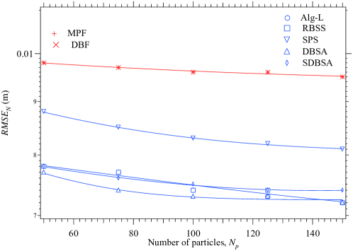
Figure 5: RMSE performance versus $N_{p}$ for the nonlinear component ($RMSE_{N}$) of the state of SSM #1; five smoothing algorithms (Alg-L, the DBSA, the SDBSA, the RBSS algorithm and the SPS algorithm) and two filtering techniques (MPF and DBF) are considered.

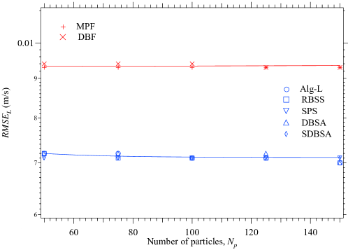
Figure 6: RMSE performance versus $N_{p}$ for the linear component ($RMSE_{L}$ ) of the state of SSM #1; five smoothing algorithms (Alg-L, the DBSA, the SDBSA, the RBSS algorithm and the SPS algorithm) and two filtering techniques (MPF and DBF) are considered.

Despite their similar accuracies, the considered smoothing algorithms require different computational efforts; this is easily inferred from the numerical results appearing in Fig. 7 and illustrating the dependence of the CTB on $N_{p}$ for all the above mentioned filtering and smoothing algorithms. In fact, these results show that CTB$($DBSA$)$ is approximately $0.85$ ($0.48$) times smaller than CTB$($Alg-L$)$ (CTB$($RBSS$)$); this is in agreement with the mathematical results illustrated in Section IV. about the complexity of Alg-L, the RBSS algorithms and the DBSA, i.e. with the fact the complexities of all these smoothers are approximately of order $\mathcal{O}(M\,N_{p}\,D_{L}^{3}T)$ (provided that $n_{i}=1$ is selected for the DBSA). Moreover, we have found that a $5.5\%$ reduction in CTB is obtained if the DDBSA is employed in place of the DBSA (i.e., if double Bayesian smoothing is not redundant). Similar considerations hold for the SDBSA, the SDDBSA and the SPS algorithm. In fact, CTB$($SDBSA$)$ is approximately $0.57$ times smaller than CTB$($SPS$)$; moreover, the CTB is reduced by $6.8\%$ if the SDDBSA is employed in place of the SDBSA. It is also interesting to note that CTB$($DBF$)$ is approximately $0.55$ times smaller than CTB$($MPF$)$ for the same value of $N_{p}$; once again, this result is in agreement with the results shown in [20] for a different SSM.

All the numerical results illustrated above lead to the conclusion that, in the considered scenario, the DDBSA and the SDDBSA achieve the best accuracy-complexity tradeoff in their categories of smoothing techniques.

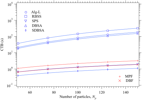
Figure 7: CTB versus $N_{p}$ for five smoothing algorithms (Alg-L, DBSA, SDBSA, the RBSS algorithm and the SPS algorithm) and two filtering techniques (MPF and DBF); SSM #1 is considered.

The second SSM we considered is the same as the second SSM illustrated in [20, Sec. IV] and refers to a sensor network employing $P$ sensors placed on the vertices of a square grid (partitioning a square area having side equal to $l$ m); these sensors receive the reference signals radiated, at the same power level and at the same frequency, by $N$ independent targets moving on a plane. Each target evolves according to the motion model described by Eqs. (120)-(121) with $\mathbf{a}_{k}(\mathbf{p}_{k})=\mathbf{0}$ for any $k$. In this case, the considered SSM (denoted SSM#2 in the following) refers to the whole set of targets and its state vector $\mathbf{x}_{k}$ results from the ordered concatenation of the vectors $\{\mathbf{x}_{k}^{(i)}$; $i=1$, $2$, $...$, $N\}$, where $\mathbf{x}_{k}^{(i)}\triangleq[(\mathbf{v}_{k}^{(i)})^{T},(\mathbf{p}_{k}^{(i)})^{T}]^{T}$, and  $\mathbf{v}_{k}^{(i)}$ and $\mathbf{p}_{k}^{(i)}$ represent the $i-$th target velocity and the position, respectively. Moreover, the following additional assumptions have been made about this SSM: 1) the process noises $\mathbf{n}_{p,k}^{(i)}$ and $\mathbf{n}_{v,k}^{(i)}$, affecting the $i-$th target position and velocity, respectively, are given by $\mathbf{n}_{p,k}^{(i)}=(T_{s}^{2}/2)\,\mathbf{n}_{a,k}^{(i)}$ and $\mathbf{n}_{v,k}^{(i)}=T_{s}\mathbf{\,n}_{a,k}^{(i)}$, where $\{\mathbf{n}_{a,k}^{(i)}\}$ is two-dimensional AWGN, representing a random acceleration and having covariance matrix $\sigma_{a}^{2}\,\mathbf{I}_{2}$ (with $i=1$, $2$, $...$, $N$); 2) the measurement acquired by the $q-$th sensor (with $q=1$, $2$, $...$, $P$) in the $k$-th observation interval is given by

$$y_{q,k}=10\,\mathrm{log}_{10}\left({\Psi}\sum_{i=1}^{N}\frac{\,d_{0}^{2}}{\left|\left|\mathbf{s}_{q}-\mathbf{p}_{k}^{(i)}\right|\right|^{2}}\right)+e_{k},$$ (124)

where the measurement noise $\{e_{k}\}$ is AWGN with variance $\sigma_{e}^{2}$, ${\Psi}$ denotes the normalised power received by each sensor from any target at a distance $d_{0}$ from the sensor itself and $\mathbf{s}_{q}$ is the position of the considered sensor; 3) the overall measurement vector $\mathbf{y}_{k}$ results from the ordered concatenation of the measurements $\{y_{q,k}$; $q=1$, $2$, $...$, $P\}$ and, consequently, provides information about the position only; 4) the initial position $\mathbf{p}_{0}^{(i)}\triangleq[p_{x,0}^{(i)},p_{y,0}^{(i)}]^{T}$ and the initial velocity $\mathbf{v}_{0}^{(i)}\triangleq[v_{x,0}^{(i)},v_{y,0}^{(i)}]^{T}$ of the $i-$th target are randomly selected (with $i=1$, $2$, $...$, $N$). As far as the last point is concerned, it is important to mention that, in our computer simulations, distinct targets are placed in different squares of the partitioned area in a random fashion; moreover, the initial velocity of each target is randomly selected within the interval $(v_{\mathrm{min}},v_{\mathrm{max}})$ in order to ensure that the trajectories of distinct targets do not cross each other in the observation interval. The following values have been selected for the parameters of SSM#2: $P=25$, $l=10^{3}$ m, $T_{s}=1$ s, $\rho=1$, $\sigma_{a}^{2}=0.1$ m/s², $\sigma_{e}^{2}=-35$ dB, ${\Psi=1}$, $d_{0}=1$ m, $v_{\mathrm{min}}=0$ m/s and $v_{\mathrm{min}}=0.1$ m/s. Moreover, $N=3$ targets have been observed over a time interval lasting $T=60$ $T_{s}$ s. Our computer simulations have aimed at evaluating the accuracy achieved by the considered smoothing algorithms in tracking the position of all the targets. In practice, such an accuracy has been assessed by estimating the average RMSE referring to the estimates of the whole set $\{\mathbf{p}_{k}^{(i)}$; $i=1$, $2$, $3\}$; note that, if the $i-$th target is considered, its position $\mathbf{p}_{k}^{(i)}$ represents the  nonlinear component of the associated substate $\mathbf{x}_{k}^{(i)}$, because of the nonlinear dependence of $\mathbf{y}_{k}$ on it (see Eq. (124)). Our computer simulations have evidenced that, in the considered scenario, the MPF and the SDBF techniques diverge frequently in the observation interval (some numerical results about the probability of divergence area available in [20, Sec. IV]); unluckily, when this occurs, all the smoothing algorithms that employ these techniques in their forward pass (namely, Alg-L, the RBSS algorithm, the SPS algorithm, the DDBSA and the SDDBSA) are unable to recover from this event and, consequently, are useless. The DBF technique, instead, thanks to its inner redundancy, is still able to track all the targets. Moreover, the two smoothing algorithms employing this technique in their forward pass (namely, the DBSA and the SDBSA), are able to improve the accuracy of position estimates in their backward pass; this is evidenced by Fig. 8, that shows the dependence of $RMSE_{N}$ on the overall number of particles ($N_{p}$) for the DBF technique, the DBSA and the SDBSA (the range $[300,600]$ is considered for $N_{p}$). Note that the SDBSA is outperformed by the DBSA in terms of $RMSE_{N}$; for instance, $RMSE_{N}($SDBSA$)$ is about $1.31$ times larger than $RMSE_{N}($DBSA$)$ for $N_{p}=500$. However, this result is achieved at the price of a significantly higher complexity; in fact, CTB$($SDBSA$)$ is approximately equal to $2\cdot 10^{-3}\cdot$CTB$($DBSA$)$.

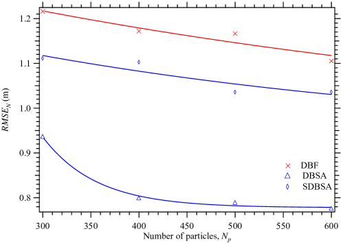
Figure 8: RMSE performance versus $N_{p}$ for the nonlinear component ($RMSE_{N}$) of the state of SSM #2; two smoothing algorithms (the DBSA and the SDBSA) and one filtering technique (DBF) are considered.

VI. Conclusions

In this manuscript, factor graph methods have been exploited to develop new smoothing algorithms based on the interconnection of two Bayesian filters in the forward pass and of two backward information filters in the backward pass. This has allowed us to develop a new approximate method for Bayesian smoothing, called double Bayesian smoothing. Four double Bayesian smoothers have been derived for the class of conditionally linear Gaussian systems and have been compared, in terms of both accuracy and execution time, with other smoothing algorithms for two specific dynamic models. Our simulation results lead to the conclusion that the devised algorithms can achieve a better complexity-accuracy tradeoff and a better tracking capability than other smoothing techniques recently appeared in the literature.

Appendix A

In this Appendix, the derivation of the expressions of various messages evaluated in each of the three phases the DBSA consists of is sketched.

Phase I - Formulas (39) and (LABEL:w_bp_x_l), referring to the message $\reflectbox{$\vec{\reflectbox{$m$}}$}_{1}(\mathbf{x}_{k})$ (38), can be easily computed by applying eqs. (IV.6)-(IV.8) of ref. [21, Table 4, p.1304] in their backward form (with $A{\rightarrow}\mathbf{I}_{D}$, $X{\rightarrow}\mathbf{F}_{k}\mathbf{x}_{k}$, $Z{\rightarrow}\mathbf{x}_{k+1}$ and $Y{\rightarrow}\mathbf{u}_{k}+\mathbf{w}_{k}$) and, then, eqs. (III.5)-(III.6) of [21, Table 3, p.1304] (with $A{\ \rightarrow}\mathbf{F}_{k}$, $X{\rightarrow}\mathbf{x}_{k}$ and $Y{\ \rightarrow}\mathbf{F}_{k}\mathbf{x}_{k}$).

Phase II -Step 1) The message $m_{2}^{(n)}(\mathbf{x}_{k})$ (42) results from merging, in the BIF${}_{2}{\rightarrow}$BIF₁ block, the statistical information about the nonlinear state component conveyed by the message $m_{1}^{(n-1)}(\mathbf{x}_{k}^{(N)})$ (41) (and, consequently, by its $N_{p}$ components $\{m_{1,j}^{(n-1)}(\mathbf{x}_{k}^{(N)})=W_{1,k,j}^{(n-1)}\,\delta(\mathbf{x}_{k}^{(N)}-\mathbf{x}_{k,j}^{(N)})\}$) with those provided by the pseudo-measurement $\mathbf{z}_{k}^{(L)}$ (21) about the  linear state component. The method employed for processing this pseudo-measurement is the same as that developed for MPF and can be summarised as follows (additional mathematical details can be found in [23, Sec. IV, p. 1527]):

1) The particles $\mathbf{x}_{k,j}^{(N)}$ and $\mathbf{x}_{\mathrm{be},k+1}^{(N)}$, conveyed by the messages $m_{1}^{(n-1)}(\mathbf{x}_{k}^{(N)})$ (41) and $\reflectbox{$\vec{\reflectbox{$m$}}$}_{\mathrm{be}}(\mathbf{x}_{k+1}^{(N)})$ (37), respectively, are employed to compute the $j-$th realization $\mathbf{z}_{k,j}^{(L)}$ (49) of $\mathbf{z}_{k}^{(L)}$ for $j=1$, $2$, $...$, $N_{p}$.

2) The pseudo-measurement $\mathbf{z}_{k,j}^{(L)}$ (49) is exploited to generate the (particle-dependent) pdf

$$f_{j}^{(n)}\left(\mathbf{x}_{k}^{(L)}\right)=\mathcal{\mathcal{N}}\left(\mathbf{x}_{k}^{(L)};\mathbf{\tilde{\eta}}_{k,j},\mathbf{\tilde{C}}_{k,j}\right),$$ (125)

that conveys pseudo-measurement information about $\mathbf{x}_{k}^{(L)}$ for any $j$; the covariance matrix $\mathbf{\tilde{C}}_{k,j}$ and the mean vector $\mathbf{\tilde{\eta}}_{k,j}$ of this message are computed on the basis of the precision matrix $\mathbf{\tilde{W}}_{k,j}$ (47) and the transformed mean vector $\mathbf{\tilde{w}}_{k,j}$ (48), respectively.

3) The messages $\{m_{1,j}^{(n-1)}(\mathbf{x}_{k}^{(N)})\}$ are merged with the pdfs $\{f_{j}^{(n)}(\mathbf{x}_{k}^{(L)})\}$ to generate the message $m_{2}^{(n)}(\mathbf{x}_{k})$ (42). The approach we adopt to achieve this result is based on the fact that the message $m_{1,j}^{(n-1)}(\mathbf{x}_{k}^{(N)})$ and the pdf $f_{j}^{(n)}(\mathbf{x}_{k}^{(L)})$ refer to the same particle (i.e., to the $j-$th particle $\mathbf{x}_{k,j}^{(N)}$, but provide complementary information (since they refer to the two different components of the overall state $\mathbf{x}_{k}$). This allows us to condense the statistical information conveyed by the sets $\{m_{1,j}^{(n-1)}(\mathbf{x}_{k}^{(N)})\}$ and $\{f_{j}^{(n)}(\mathbf{x}_{k}^{(L)})\}$ in the joint pdf

$$f^{(n)}(\mathbf{x}_{k}^{(L)},\mathbf{x}_{k}^{(N)})\triangleq w_{p}\sum\limits_{j=1}^{N_{p}}m_{1,j}^{(n-1)}\left(\mathbf{x}_{k}^{(N)}\right)\,f_{j}^{(n)}\left(\mathbf{x}_{k}^{(L)}\right).$$ (126)

referring to the whole state $\mathbf{x}_{k}$. Then, the message $m_{2}^{(n)}(\mathbf{x}_{k})$ (42) is computed by projecting the pdf $f^{(k)}(\mathbf{x}_{k}^{(L)},\mathbf{x}_{k}^{(N)})$ (126) onto a single Gaussian pdf having the same mean and covariance.

Steps 2 and 3) The expression (52) of $\reflectbox{$\vec{\reflectbox{$m$}}$}_{3}^{(n)}\left(\mathbf{x}_{k}\right)$ represents a straightforward application of formula no. 2 of ref. [23, App. A, TABLE I] (with $\mathbf{W}_{1}{\rightarrow}\mathbf{W}_{1,k}$, $\mathbf{W}_{2}{\rightarrow}\mathbf{W}_{2,k}^{(n)}$, $\mathbf{w}_{1}{\rightarrow}\mathbf{w}_{1,k}$ and $\mathbf{w}_{2}{\rightarrow}\mathbf{w}_{2,k}^{(n)}$). The same considerations apply to the derivation of the expression (58) of $m_{4}^{(n)}\left(\mathbf{x}_{k}\right)$.

Step 4) The expression (63) of the weight $w_{3,k,j}^{(n)}$ is derived as follows. First, we substitute the expression (LABEL:f_x_N) of $f(\mathbf{x}_{k+1}^{(N)}|\mathbf{x}_{k}^{(N)},\mathbf{x}_{k}^{(L)})$, and the expressions of the messages $\reflectbox{$\vec{\reflectbox{$m$}}$}_{be}(\mathbf{x}_{k+1}^{(N)})$ (37) and $m_{1}^{(n)}(\mathbf{x}_{k}^{(L)})$ (61) in the right-hand side (RHS) of Eq. (62). Then, the resulting integral is solved by applying formula no. 1 of [23, App. A, TABLE II] in the integration with respect to $\mathbf{x}_{k}^{(L)}$ and the sifting property of the Dirac delta function in the integration with respect to $\mathbf{x}_{k+1}^{(N)}$.

Step 5) - The derivation of the expression (68) of the weight $w_{2,k,j}^{(n)}$ is similar to that illustrated for the particle weights originating from the pseudo-measurements in dual MPF and can be summarised as follows (additional mathematical details can be found in ref. [23, Sec. V, pp. 1528-1529]). Two different Gaussian densities are derived for the random vector $\mathbf{z}_{k}^{(N)}$ (24), conditioned on $\mathbf{x}_{k}^{(N)}$. The expression of the first density originates from the definition (24) and from the knowledge of the joint pdf of $\mathbf{x}_{k}^{(L)}$ and $\mathbf{x}_{k+1}^{(L)}$; this joint density is obtained from: a) the statistical information provided by the message $m_{1}^{(n)}(\mathbf{x}_{k}^{(L)})$ (61) and the pdf $\mathcal{\mathcal{N}}(\mathbf{x}_{k+1}^{(L)},\mathbf{\tilde{\eta}}_{\mathrm{be},k+1}\mathbf{\tilde{C}}_{\mathrm{be},k+1})$ (resulting from integrating out the dependence of $\reflectbox{$\vec{\reflectbox{$m$}}$}_{\mathrm{be}}(\mathbf{x}_{k+1})$ (36) on $\mathbf{x}_{k}^{(N)}$); b) the Markov model $f(\mathbf{x}_{k+1}^{(L)}|\mathbf{x}_{k}^{(N)},\mathbf{x}_{k}^{(L)})$ (LABEL:f_x_L). This leads to the pdf

$$f_{1}^{(n)}\left(\mathbf{z}_{k}^{(N)}\left|\mathbf{x}_{k}^{(N)}\right.\right)=\mathcal{N}\left(\mathbf{z}_{k}^{(N)};\mathbf{\check{\eta}}_{z,k}^{(n)}\left(\mathbf{x}_{k}^{(N)}\right),\mathbf{\check{C}}_{z,k}^{(n)}\left(\mathbf{x}_{k}^{(N)}\right)\right),$$ (127)

where

$$\mathbf{\check{\eta}}_{z,k}^{(n)}\left(\mathbf{x}_{k}^{(N)}\right)=\mathbf{\ \tilde{\eta}}_{\mathrm{be},k+1}-\mathbf{A}_{k}^{(L)}\left(\mathbf{x}_{k}^{(N)}\right)\,\mathbf{\tilde{\eta}}_{1,k}^{(n)}$$ (128)

and

$$\mathbf{\check{C}}_{z,k}^{(n)}\left(\mathbf{x}_{k}^{(N)}\right)=\mathbf{\ \tilde{C}}_{\mathrm{be},k+1}-\mathbf{A}_{k}^{(L)}\left(\mathbf{x}_{k}^{(N)}\right)\mathbf{\tilde{C}}_{1,k}^{(n)}\,\left(\mathbf{A}_{k}^{(L)}\left(\mathbf{x}_{k}^{(N)}\right)\right)^{T}.$$ (129)

The second pdf of $\mathbf{z}_{k}^{(N)}$, instead, results from the fact that this vector $\mathbf{z}_{k}^{(N)}$ must equal the sum (25); consequently, it is given by

$$f_{2}\left(\mathbf{z}_{k}^{(N)}\left|\mathbf{x}_{k}^{(N)}\right.\right)=\mathcal{N}\left(\mathbf{z}_{k}^{(N)};\mathbf{f}_{k}^{(L)}\left(\mathbf{x}_{k}^{(N)}\right),\mathbf{C}_{w}^{(N)}\right).$$ (130)

Given the pdfs (127) and (130), the message $\vec{m}_{3}^{(n)}(\mathbf{x}_{k}^{(N)})$ is expressed by their correlation, i.e. it is computed as

$$\vec{m}_{3}^{(n)}(\mathbf{x}_{k}^{(N)}) = \int f_{1}^{(n)}\left(\mathbf{z}_{k}^{(N)}\left|\mathbf{x}_{k}^{(N)}\right.\right)\cdot f_{2}\left(\mathbf{z}_{k}^{(N)}\left|\mathbf{x}_{k}^{(N)}\right.\right)d\mathbf{z}_{k}^{(N)}.$$ (131)

Substituting Eqs. (127) and (130) in the RHS of the last expression, setting $\mathbf{x}_{k}^{(N)}=\mathbf{x}_{k,j}^{(N)}$ and applying formula no. 4 of ref. [23, Table II] to the evaluation of the resulting integral yields Eq. (68); note that $\mathbf{\ \check{\eta}}_{z,k,j}^{(n)}$ (70) and $\mathbf{\check{C}}_{z,k,j}^{(n)}$ (71) represent the values taken on by $\mathbf{\check{\eta}}_{z,k}^{(n)}(\mathbf{x}_{k}^{(N)})$ (128) and $\mathbf{\check{C}}_{z,k}^{(n)}(\mathbf{x}_{k}^{(N)})$ (129), respectively, for $\mathbf{x}_{k}^{(N)}=\mathbf{x}_{k,j}^{(N)}$.

Step 7) The expression (82) of the weight $w_{5,k,j}^{(n)}$ is derived as follows. First, we substitute the expressions (61) and (20) of $m_{1}^{(n)}(\mathbf{x}_{k}^{(L)})$ and $f(\mathbf{y}_{k}|\mathbf{x}_{k}^{(N)},\,\mathbf{x}_{k}^{(L)})$, respectively, in the RHS of Eq. (C.). Then, solving the resulting integral (see formula no. 1 of ref. [23, App. A, TABLE II]) produces Eq. (LABEL:eq:weight_before_resampling). Finally, setting $\mathbf{x}_{k}^{(N)}=\mathbf{x}_{k,j}^{(N)}$ in Eq. (LABEL:eq:weight_before_resampling) yields Eq. (82).

Phase III - The expression (100) of the message $\reflectbox{$\vec{\reflectbox{$m$}}$}_{\mathrm{be}}\left(\mathbf{x}_{k}\right)$ results from the application of formula no. 2 of ref. [23, App. A, TABLE I] to Eq. (99).

Appendix B Computational complexity of the devised double
Bayesian smoothers

In this appendix, the computational complexity of the tasks accomplished in a single recursion of backward filtering and smoothing of the DBSA is assessed in terms of flops. Moreover, we comment on how the illustrated results can be also exploited to assess the computational complexity of a single recursion of the DDBSA. In the following, $\mathcal{C}_{\mathbf{H}}$, $\mathcal{C}_{\mathbf{B}}$, $\mathcal{C}_{\mathbf{F}}$, $\mathcal{C}_{\mathbf{A}^{(L)}}$ and $\mathcal{C}_{\mathbf{A}^{(N)}}$, and $\mathcal{C}_{\mathbf{g}}$, $\mathcal{C}_{\mathbf{f}^{(L)}}$, $\mathcal{C}_{\mathbf{f}^{(N)}}$ and $\mathcal{C}_{\mathbf{f}_{k}}$denote the cost due to the evaluation of the matrices $\mathbf{H}_{k}$, $\mathbf{B}_{k}$, $\mathbf{F}_{k}$, $\mathbf{A}_{k}^{(L)}(\mathbf{x}_{k}^{(N)})$ and $\mathbf{A}_{k}^{(N)}(\mathbf{x}_{k}^{(N)})$, and of the functions $\mathbf{g}_{k}(\mathbf{x}_{k}^{(N)})$, $\mathbf{f}_{k}^{(L)}(\mathbf{x}_{k}^{(N)})$, $\mathbf{f}_{k}^{(N)}(\mathbf{x}_{k}^{(N)})$ and $\mathbf{f}_{k}(\mathbf{x}_{k})$, respectively. Moreover, similarly as [26], it is assumed that the computation of the inverse of any covariance matrix involves a Cholesky decomposition of the matrix itself and the inversion of a lower or upper triangular matrix. Finally, it is assumed that the computation of the determinant of any matrix involves a Cholesky decomposition of the matrix itself and the product of the diagonal entries of a triangular matrix.

Phase I - The overall computational cost of this task is evaluated as (see Eqs. (39)-(LABEL:w_bp_x_l) and (47)-(49))

$$\mathcal{C}_{1} = \mathcal{C}_{\mathbf{W}_{1,k}}+\mathcal{C}_{\mathbf{w}_{1,k}}+N_{p}\left(\mathcal{C}_{\mathbf{z}_{k,j}^{(L)}}+\mathcal{C}_{\mathbf{\tilde{W}}_{k,j}}\right.$$ (132)

$$\left.+\mathcal{C}_{\mathbf{\tilde{w}}_{k,j}}+\mathcal{C}_{\mathbf{\tilde{C}}_{k,j}}+\mathcal{C}_{\tilde{\eta}_{k,j}}\right)\triangleq\mathcal{C}_{\mathrm{bp}}^{(1)}.$$

Moreover, we have that: 1) the cost $\mathcal{C}_{\mathbf{W}_{1,k}}$ is equal to $\mathcal{C}_{\mathbf{F}}+26D^{3}/3-D^{2}/2+5D/6$ flops; 2) the cost $\mathcal{C}_{\mathbf{w}_{1,k}}$ is equal to $4D^{3}+4D^{2}-2D$ flops (the cost for computing $\mathcal{C}_{\mathbf{F}}$ has been already accounted for at point 1)); 3) the cost $\mathcal{C}_{\mathbf{z}_{k,j}^{(L)}}$ is equal to $\mathcal{C}_{\mathbf{f}^{(N)}}+D_{N}$ flops; 4) the cost $\mathcal{C}_{\mathbf{\tilde{W}}_{k,j}}$ is equal to $\mathcal{C}_{\mathbf{A}^{(N)}}+4D_{N}^{3}-2D_{N}^{2}$ flops; 5) the cost $\mathcal{C}_{\mathbf{\tilde{w}}_{k,j}}$ is equal to $2D_{N}^{3}+D_{N}^{2}-D_{N}$ flops (the cost for computing $\mathcal{C}_{\mathbf{A}^{(N)}}$ has been already accounted for at point 4)); 6) the cost $\mathcal{C}_{\mathbf{\tilde{C}}_{k,j}}$ is equal to $2D_{N}^{3}/3+3D_{N}^{2}/2+5D_{N}/6$ flops; 7) the cost $\mathcal{C}_{\tilde{\eta}_{k,j}}$ is equal to $2D_{N}^{2}-D_{N}$ flops. The expressions listed at points 1)-2) can be exploited for the DDBSA too; in the last case, however, $D_{N}=0$ and $D=D_{L}$ must be assumed.

Phase II - The overall computational cost of this task is evaluated as

$$\mathcal{C}_{2} = n_{i}\left(\mathcal{C}_{\mathrm{pm}^{(1)}}+\mathcal{C}_{\mathrm{be}1^{(1)}}+\mathcal{C}_{\mathrm{sm}^{(1)}}+\mathcal{C}_{\mathrm{bp}^{(2)}}+\right.$$ (133)

$$\left.\mathcal{C}_{\mathrm{pm}^{(2)}}+\mathcal{C}_{\mathrm{ms}^{(2)}}+\mathcal{C}_{\mathrm{be}2^{(2)}}+\mathcal{C}_{\mathrm{sm}^{(2)}}\right).$$

The terms appearing in the RHS of the last equation can be computed as follows. First of all, we have that

$$\mathcal{C}_{\mathrm{pm}^{(1)}}=\mathcal{C}_{\eta_{2,k}^{(n)}}+\mathcal{C}_{\mathbf{C}_{2,k}^{(n)}},$$ (134)

where (see Eqs. (43)-(44)): 1) the cost $\mathcal{C}_{\eta_{2,k}^{(n)}}$ is equal to $2N_{p}D-D$ flops; 2) the cost $\mathcal{C}_{\mathbf{C}_{2,k}^{(n)}}$ is equal to $5N_{p}D_{L}^{2}+4N_{p}D_{N}^{2}+4N_{p}D_{L}D_{N}+D_{L}^{2}+D_{N}^{2}+D_{L}D_{N}$ flops. The expressions listed at points 1)-2) can be exploited for the DDBSA too; in the last case, however, $D_{N}=0$ and $D=D_{L}$ must be assumed.

The second term appearing in the RHS of Eq. (133) is evaluated as

$$\mathcal{C}_{\mathrm{be}1^{(1)}}=\mathcal{C}_{\mathbf{C}_{3,k}^{(n)}}+\mathcal{C}_{\eta_{3,k}^{(n)}}+\mathcal{C}_{\mathbf{W}_{3,k}^{(n)}}+\mathcal{C}_{\mathbf{w}_{3,k}^{(n)}},$$ (135)

where (see Eqs. (55)-(56)): 1) the cost $\mathcal{C}_{\mathbf{C}_{3,k}^{(n)}}$ is equal to $14D^{3}/3+D^{2}/2+5D/6$ flops; 2) the cost $\mathcal{C}_{\eta_{3,k}^{(n)}}$ is equal to $4D^{2}-D$ flops (the cost for computing $\mathcal{C}_{\mathbf{W}_{k}^{(n)}}$ has been already accounted for at point 1)); 3) the cost $\mathcal{C}_{\mathbf{W}_{3,k}^{(n)}}$ is equal to $2D^{3}/3+3D^{2}/2+5D/6$ flops; 4) the cost $\mathcal{C}_{\mathbf{w}_{3,k}^{(n)}}$ is equal to $2D^{2}-D$ flops. The expressions listed at points 1)-4) can be exploited for the DDBSA too; in the last case, however, $D_{N}=0$ and $D=D_{L}$ must be assumed.

The third term appearing in the RHS of Eq. (133) is computed as

$$\mathcal{C}_{\mathrm{sm}^{(1)}}=\mathcal{C}_{\mathbf{W}_{4,k}^{(n)}}+\mathcal{C}_{\mathbf{w}_{4,k}^{(n)}}+\mathcal{C}_{\mathbf{C}_{4,k}^{(n)}}+\mathcal{C}_{\eta_{4,k}^{(n)}},$$ (136)

where (see Eqs. (59)-(60)): 1) the cost $\mathcal{C}_{\mathbf{W}_{4,k}^{(n)}}$ is equal to $D^{2}$ flops; 2) the cost $\mathcal{C}_{\mathbf{w}_{4,k}^{(n)}}$ is equal to $D$ flops; 3) the cost $\mathcal{C}_{\mathbf{C}_{4,k}^{(n)}}$ is equal to $2D^{3}/3+3D^{2}/2+5D/6$ flops; 4) the cost $\mathcal{C}_{\eta_{4,k}^{(n)}}$ is equal to $2D^{2}-D$ flops. The expressions listed at points 1)-4) can be exploited for the DDBSA too; in the last case, however, $D_{N}=0$ and $D=D_{L}$ must be assumed.

The fourth term appearing in the RHS of Eq. (133) is given by

$$\mathcal{C}_{\mathrm{bp}^{(2)}}=N_{p}\left(\mathcal{C}_{\eta_{3,k,j}^{(N)}}+\mathcal{C}_{\mathbf{C}_{3,k,j}^{(N)}}+\mathcal{C}_{D_{3,k,j}^{(n)}}+\mathcal{C}_{Z_{3,k,j}^{(n)}}\right),$$ (137)

where (see Eqs. (66)-(67) and (64)-(65)): 1) the cost $\mathcal{C}_{\eta_{3,k,j}^{(N)}}$ is equal to $\mathcal{C}_{\mathbf{A}^{(N)}}+\mathcal{C}_{\mathbf{f}^{(N)}}+2D_{L}D_{N}$ flops; 2) the cost $\mathcal{C}_{\mathbf{C}_{3,k,j}^{(N)}}$ is equal to $2D_{L}^{2}D_{N}+2D_{L}D_{N}^{2}-D_{L}D_{N}$ flops (the cost for computing $\mathcal{C}_{\mathbf{A}^{(N)}}$ and $\mathcal{C}_{\mathbf{f}^{(N)}}$ has been already accounted for at point 1)); 3) the cost $\mathcal{C}_{D_{3,k,j}^{(n)}}$ is equal to $D_{N}^{3}/3+D_{N}^{2}+5D_{N}/3+2$ flops; 4) the cost $\mathcal{C}_{Z_{3,k,j}^{(n)}}$ is equal to $2D_{N}^{2}+2D_{N}-1$ flops.

The fifth term appearing in the RHS of Eq. (133) is evaluated as

$$\mathcal{C}_{\mathrm{pm}^{(2)}} = N_{p}\left(\mathcal{C}_{\check{\eta}_{z,k,j}^{(n)}}+\mathcal{C}_{\mathbf{\check{C}}_{z,k,j}^{(n)}}+\mathcal{C}_{\mathbf{\check{W}}_{2,k,j}^{(n)}}+\mathcal{C}_{\mathbf{\check{w}}_{2,k,j}^{(n)}}+\mathcal{C}_{D_{2,k,j}^{(n)}}+\mathcal{C}_{Z_{2,k,j}^{(n)}}\right),$$ (138)

where (see Eqs. (69)-(74)): 1) the cost $\mathcal{C}_{\check{\eta}_{z,k,j}^{(n)}}$ is equal to $\mathcal{C}_{\mathbf{A}^{(L)}}+2D_{L}^{2}$ flops; 2) the cost $\mathcal{C}_{\mathbf{\check{C}}_{z,k,j}^{(n)}}$ is equal to $4D_{L}^{3}-D_{L}^{2}$ flops (the cost for computing $\mathcal{C}_{\mathbf{A}^{(L)}}$ has been already accounted for at point 1)); 3) the cost $\mathcal{C}_{\mathbf{\check{W}}_{2,k,j}^{(n)}}$ is equal to $2D_{L}^{3}/3+5D_{L}^{2}/2+5D_{L}/6$ flops; 4) the cost $\mathcal{C}_{\mathbf{\check{w}}_{2,k,j}^{(n)}}$ is equal to $\mathcal{C}_{\mathbf{f}^{(L)}}+4D_{L}^{2}-D_{L}$ flops; 5) the cost $\mathcal{C}_{D_{2,k,j}^{(n)}}$ is equal to $D_{L}^{3}/3+2D_{L}^{2}+5D_{L}/3+2$ flops; 6) the cost $\mathcal{C}_{Z_{2,k,j}^{(n)}}$ is equal to $6D_{L}^{2}+3D_{L}-1$ flops.

The sixth term appearing in the RHS of Eq. (133) is computed as

$$\mathcal{C}_{\mathrm{ms}^{(2)}}=N_{p}\left(\mathcal{C}_{\bar{\eta}_{5,k,j}^{(n)}}+\mathcal{C}_{\mathbf{\bar{C}}_{5,k,j}^{(n)}}+\mathcal{C}_{D_{5,k,j}^{(n)}}+\mathcal{C}_{Z_{5,k,j}^{(n)}}\right),$$ (139)

where (see Eqs. (83)-(86)): 1) the cost $\mathcal{C}_{\bar{\eta}_{5,k,j}^{(n)}}$ is equal to $\mathcal{C}_{\mathbf{B}}+\mathcal{C}_{\mathbf{g}}+2PD_{L}$ flops; 2) the cost $\mathcal{C}_{\mathbf{\bar{C}}_{5,k,j}^{(n)}}$ is equal to $2PD_{L}^{2}+2P^{2}D_{L}-PD_{L}$ flops (the cost for computing $\mathcal{C}_{\mathbf{B}}$ has been already accounted for at point 1)); 3) the cost $\mathcal{C}_{D_{5,k,j}^{(n)}}$ is equal to $D_{L}^{3}/3+D_{L}^{2}+5D_{L}/3+2$ flops; 4) the cost $\mathcal{C}_{Z_{5,k,j}^{(n)}}$ is equal to $2P^{3}/3+7P^{2}/2+17P/6-1$ flops. It is important to note that, if the forward weights $\{w_{\mathrm{fe},k,j}\}$ are reused, the cost $\mathcal{C}_{\mathrm{ms}^{(2)}}$ appearing in Eq. (139) is equal to zero.

The seventh term appearing in the RHS of Eq. (133) is given by

$$\mathcal{C}_{\mathrm{be}2^{(2)}}=N_{p}\left(\mathcal{C}_{D_{6,k,j}^{(n)}}+\mathcal{C}_{Z_{6,k,j}^{(n)}}+\mathcal{C}_{w_{6,k,j}^{(n)}}\right),$$ (140)

where the costs $\mathcal{C}_{D_{6,k,j}^{(n)}}$ and $\mathcal{C}_{Z_{6,k,j}^{(n)}}$ are equal to $2$ flops, and the cost $\mathcal{C}_{w_{6,k,j}^{(n)}}$ is equal to $3$ flops (see Eqs. (89)-(91)). If the forward weights $\{w_{\mathrm{fe},k,j}\}$ are reused, the costs $\mathcal{C}_{D_{6,k,j}^{(n)}}$ and $\mathcal{C}_{Z_{6,k,j}^{(n)}}$ are equal to $1$ flops, whereas the cost $\mathcal{C}_{w_{6,k,j}^{(n)}}$ remains unchanged.

The last term appearing in the RHS of Eq. (133) is evaluated as

$$\mathcal{C}_{\mathrm{sm}^{(2)}}=\mathcal{C}_{w_{1,k,j}^{(n)}}+\mathcal{C}_{W_{1,k,j}^{(n)}},$$ (141)

where the costs $\mathcal{C}_{w_{1,k,j}^{(n)}}$ and $\mathcal{C}_{W_{1,k,j}^{(n)}}$ are equal to $N_{p}$ and $2N_{p}-1$ flops, respectively (see Eqs. (95)-(96)).

Phase III - The overall computational cost of this task is evaluated as

$$\mathcal{C}_{3}=\mathcal{C}_{\mathrm{be}^{(2)}}+\mathcal{C}_{\mathrm{pm}^{(1)}}+\mathcal{C}_{\mathrm{be}1^{(1)}}+\mathcal{C}_{\mathrm{be}^{(1)}}.$$ (142)

Here, the cost $\mathcal{C}_{\mathrm{be}^{(2)}}$ is equal to $\mathcal{C}_{S}(N_{p})$, that represents the total cost of a sampling step that involves a particle set of size $N_{p}$; moreover, the costs $\mathcal{C}_{\mathrm{pm}^{(1)}}$ and $\mathcal{C}_{\mathrm{be}1^{(1)}}$ are the same as those appearing in the RHS of Eq. (133), and $\mathcal{C}_{\mathrm{be}^{(1)}}$ is computed as (see Eqs. (102)-(105))

$$\mathcal{C}_{\mathrm{be}^{(1)}} = \mathcal{C}_{\mathbf{W}_{\mathrm{ms},k}}+\mathcal{C}_{\mathbf{w}_{\mathrm{ms},k}}+\mathcal{C}_{\mathbf{W}_{\mathrm{be}2,k}}+$$

$$\mathcal{C}_{\mathbf{w}_{\mathrm{be}2,k}}+\mathcal{C}_{\mathbf{C}_{\mathrm{be}}}+\mathcal{C}_{\eta_{\mathrm{be}}}.$$

Moreover, we have that: 1) the cost $\mathcal{C}_{\mathbf{W}_{\mathrm{ms},k}}$ is equal to $\mathcal{C}_{\mathbf{H}}+2P^{2}D+2PD^{2}-D^{2}-PD$ flops; 2) the cost $\mathcal{C}_{\mathbf{w}_{\mathrm{ms},k}}$ is equal to $\mathcal{C}_{\mathbf{B}}+\mathcal{C}_{\mathbf{g}}+2P^{2}D+3PD+2PD_{L}-P-D$ flops (the cost for computing $\mathcal{C}_{\mathbf{H}}$ has been already accounted for at point 1)); 3) the cost $\mathcal{C}_{\mathbf{W}_{\mathrm{be}2,k}}$ is equal to $D^{2}$ flops; 4) the cost $\mathcal{C}_{\mathbf{w}_{\mathrm{be}2,k}}$ is equal to $D$ flops; 5) the cost $\mathcal{C}_{\mathbf{C}_{\mathrm{be}}}$ is equal to $2D^{3}/3+3D^{2}/2+5D/6$ flops; 6) the cost $\mathcal{C}_{\eta_{\mathrm{be}}}$ is equal to $2D^{2}-D$ flops. The expressions listed at points 1)-6) can be exploited for the DDBSA too; in the last case, however, $D_{N}=0$ and $D=D_{L}$ must be assumed. Note that the costs $\mathcal{C}_{\mathbf{W}_{\mathrm{ms},k}}$ and $\mathcal{C}_{\mathbf{w}_{\mathrm{ms},k}}$ (see points 1) and 2)) are ignored if the precision matrix $\mathbf{W}_{\mathrm{ms},k}$ and the transformed mean vector $\mathbf{w}_{\mathrm{ms},k}$ are stored in the forward pass (so that they do not need to be recomputed in the backward pass). Moreover, if the SDBSA or the SDDBSA is used, the cost $\mathcal{C}_{\mathrm{be}^{(2)}}$ in the RHS of Eq. (142) becomes $D_{N}(2N_{p}-1)$ flops.

Finally, it is worth stressing that, if the DBSA or the DDBSA (the SDBSA or the SDDBSA) is employed, the overall computational complexity is obtained by multiplying the computational cost assessed for a single recursion by $M\,T$ (by $T$), where $M$ and $T$ denote the overall number of accomplished backward passes and the duration of the observation interval, respectively.

References

- [1] B. Anderson and J. Moore, Optimal Filtering, Englewood Cliffs, NJ, Prentice-Hall, 1979.
- [2] S. Särkkä, Bayesian Filtering and Smoothing. Cambridge, U.K.: Cambridge Univ. Press, 2013.
- [3] A. Doucet, S. Godsill and C. Andrieu, “On Sequential Monte Carlo Sampling Methods for Bayesian Filtering”, Statist. Comput., vol. 10, no. 3, pp. 197-208, 2000.
- [4] G. Kitagawa, “Non-Gaussian state-space modeling of nonstationary time series”, Journal of the American Statistical Association, vol. 82, pp. 1032-1063, 1987.
- [5] G. Kitagawa, “The two-filter formula for smoothing and an implementation of the Gaussian-sum smoother”, Annals of the Institute of Statistical Mathematics, vol. 46, pp. 605-623, 1994.
- [6] Y. Bresler, “Two-filter formula for discrete-time non-linear Bayesian smoothing”, Int. Journal of Control, vol. 43, no. 2, pp. 629-641, 1986.
- [7] B. N. Vo, B. T. Vo and R. P. S. Mahler, “Closed-Form Solutions to Forward–Backward Smoothing”, IEEE Trans. Sig. Proc., vol. 60, no. 1, pp. 2-17, Jan. 2012.
- [8] S. Särkkä and J. Hartikainen, “On Gaussian optimal smoothing of non-linear state space models”, IEEE Trans. Autom. Control, vol. 55, no. 8, pp. 1938–1941, Aug. 2010.
- [9] J. Kokkala, A. Solin, and S. Särkkä, “Sigma-point filtering and smoothing-based parameter estimation in nonlinear dynamic systems”, J. Adv. Inf. Fusion, vol. 11, no. 1, pp. 15–30, 2016.
- [10] A. F. García-Fernández, L. Svensson and S. Särkkä, “Iterated posterior linearisation smoother”, IEEE Trans. Autom. Control, vol. 62, no. 4, pp. 2056–2063, Apr. 2017.
- [11] R. Doucet, A. Garivier, E. Moulines and J. Olsson, “Sequential Monte Carlo smoothing for general state space hidden Markov models”, Ann. Appl. Probab., vol. 21, no. 6, pp. 2109–2145, 2011.
- [12] G. Kitagawa, “Monte Carlo filter and smoother for non-Gaussian nonlinear state space models”, J. Comput. Graph. Statist., vol. 5, no. 1, pp. 1–25, 1996.
- [13] S. J. Godsill, A. Doucet, and M. West, “Monte Carlo smoothing for nonlinear time series”, J. Amer. Statist. Assoc., vol. 99, no. 465, pp. 156–168, Mar. 2004.
- [14] F. Lindsten and T. B. Schön, “Backward simulation methods for Monte Carlo statistical inference”, Foundat. Trends Mach. Learn., vol. 6, no. 1, pp. 1–143, 2013.
- [15] R. Hostettler and S. Särkkä, “Rao–Blackwellized Gaussian Smoothing”, IEEE Trans. Autom. Control, vol. 64, no. 1, pp. 305-312, Jan. 2019.
- [16] M. Briers, A. Doucet and S. Maskell, “Smoothing algorithms for state-space models”, Ann. Inst. Statist. Math., vol. 62, no. 1, pp. 61–89, Feb. 2010.
- [17] W. Fong, S. J. Godsill, A. Doucet and M. West, “Monte Carlo smoothing with application to audio signal enhancement”, IEEE Trans. Signal Process., vol. 50, no. 2, pp. 438–449, Feb. 2002.
- [18] F. Lindsten, P. Bunch, S. Särkkä, T. B. Schön and S. J. Godsill, “Rao-Blackwellized Particle Smoothers for Conditionally Linear Gaussian Models”, IEEE J. Sel. Topics in Sig. Proc., vol. 10, no. 2, pp. 353-365, March 2016.
- [19] G. M. Vitetta, E. Sirignano and F. Montorsi, “Particle Smoothing for Conditionally Linear Gaussian Models as Message Passing over Factor Graphs”, IEEE Trans. Sig. Proc., vol. 66, no. 14, pp. 3633-3648, July 2018.
- [20] G. M. Vitetta, P. Di Viesti and E. Sirignano, “Multiple Bayesian Filtering as Message Passing”, submitted to the IEEE Trans. Sig. Proc., February 2019 (available on arXiv at https://arxiv.org/abs/1907.01358)
- [21] H.-A. Loeliger, J. Dauwels, Junli Hu, S. Korl, Li Ping, F. R. Kschischang, “The Factor Graph Approach to Model-Based Signal Processing”, IEEE Proc., vol. 95, no. 6, pp. 1295-1322, June 2007.
- [22] F. R. Kschischang, B. Frey, and H. Loeliger, “Factor Graphs and the Sum-Product Algorithm”, IEEE Trans. Inf. Theory, vol. 41, no. 2, pp. 498-519, Feb. 2001.
- [23] G. M. Vitetta, E. Sirignano, P. Di Viesti and F. Montorsi, “Marginalized Particle Filtering and Related Techniques as Message Passing”, IEEE Trans. Sig. Proc., vol. 67, no. 6, pp. 1522-1535, Mar. 2019.
- [24] T. Schön, F. Gustafsson, P.-J. Nordlund, “Marginalized Particle Filters for Mixed Linear/Nonlinear State-Space Models”, IEEE Trans. Sig. Proc., vol. 53, no. 7, pp. 2279-2289, July 2005.
- [25] M. S. Arulampalam, S. Maskell, N. Gordon and T. Clapp, “A Tutorial on Particle Filters for Online Nonlinear/Non-Gaussian Bayesian Tracking”, IEEE Trans. Sig. Proc., vol. 50, no. 2, pp. 174-188, Feb. 2002.
- [26] B. Ait-El-Fquih and I. Hoteit, “A variational Bayesian multiple particle filtering scheme for large-dimensional systems”, IEEE Trans. Sig. Proc., vol. 64, no. 20, pp. 5409–5422, Oct. 2016.