CASCADE CALCULATION WITH SCHEMATIC INTERACTIONS

1 Abstract

In previous works we considered schematic Hamiltonians represented by simplified matrices. We defined 2 transition operators and calculated transition strengths from the ground state to all exited states.In many cases the strengths decreased nearly exponentially with excitation energy. Now we do the reverse We start with the highest energy state and calculate the cascade of transitions until the ground states is reached.On a log plot we show the average transition strength as a function of the number of energy intervals that were crossed. We give an analytic proof of exponential behavior for transition strength in the weak coupling limit for the T₂ transition operator.

2 Introduction

In ref [1] and [2] A.Kingan et al. calculated M1 transition from the lowest J=1+ state of a selected even-even nucleus to excited states. In the first work they emphasized strong transitions to individual states.. Although transitions to the ground state were large (inverted scissors) there were many other transition strengths that were even larger i.e to other J=0+ states and to many J=2+states. Basically they were calculating double magnetic dipole strength.

In Ref [2] transitions to nearly all states we’re considered-strong or weak. A wide spread of results was noted. However when the transition strengths in certain energy intervals (bins)were summed up one saw an exponential decrease in strength with excitation energy. Coincidentally a similar behavior, exponential decrease with excitation energy, was also found in a different problem - a study of schematic matrix hamiltonians for their own sake[3,4,5].The study was mainly on tridiagonal matrices[3,4] but also later pentadiagonal were considered[5]. We will here consider also heptadiagonal matrices.

We were informed about experiments and calculations which do the opposite of what we have done-start with the highest level and calculate all transition strengths as the nucleus deexcites emitting gamma rays [6-11]. They plot the average M1 strength versus gamma ray energy. They find a strong increase in average M1 strength as one goes to low gamma ray energies.

We will here also do such calculations with our schematic Hamiltonian matrices. Because they are simpler perhaps we can cast some light on what is causing the behaviors that have been observed. Indeed in ref [5] we were able to get some analytic results for wave functions and transitions from the ground state, especially in the weak coupling limit. in contrast to [6] and [8-12] we present our results as log plots. Brown and Larsen also used a log plot [7]. It should be made clear that our basic aim is to study the properties of the matrix Hamiltonian of Table 1. We will not attempt to fit the results of [6-12] but we will see if there are some common features that might be of interest.

In a previous work [5] with tridiagonal matrices it was shown that in the weak coupling limit the ground state column vector (a₀,a₁…a_n….) was such that a_n=$(\frac{-v}{E})^{n}\frac{1}{n!}$. We recognized this as an a expansions in a Taylor series of e${}^{-\frac{v}{E}}$. The $\frac{1}{n!}$ terms come from energy denominators in the wave function

$\Psi$= $\varPhi$ + $\frac{1}{E_{0}-H_{0}}$QV$\varPsi$ = (1+$\frac{1}{E_{0}-H_{0}}$QV +$\frac{1}{E_{0}-H_{0}}$QV$\frac{1}{E_{0}-H_{0}}$QV+….. )$\varPhi$

3 The Calculation.

We here show a 11 by 11 Hepta diagonal matrix we will be working with. We can also get results for tri and penta diagonal matrices by setting certain parameters to zero.

Table 1: The septa- diagonal matrix

0	v	w	x
v	E	v	w	x
w	v	2E	v	w	x
x	w	v	3E	v	w	x
	x	w	v	4E	v	w	x
		x	w	v	5E	v	w	x
			x	w	v	6E	v	w	x
				x	w	v	7E	v	w	x
					x	w	v	8E	v	w
						x	w	v	9E	v
							x	w	v	10E

We will be considering and comparing results for tridiagonal, pentadiagonal and heptadiagonal matrix Hamiltoninans. For tridiagonal case, we set x=0, w=0 and for the pentadiagonal case, x=0 in the matrix shown in Table 1. In previous works [3,4,5] we defined 2 types of transition operators <n T₁(n+1)>= 1 and < n T₂ (n+1) > = $\sqrt{n+1}$. In this work we will only show results for the latter.

4 The Figures

We here present several figures. We only include the T₂ coupling case. We show side by side figures of the cascade down average strength (left) and the transition strength up (right). This is done first for the tridiagonal case with v=0.01, 0.1 and 1. Next for the petadiagonal case w=v(0.01, 0.1). Next heptadiagonal with v=w=x(0.01, 0.1, 1) and then again heptadiagonal w=$\frac{v}{2\!}$,x=$\frac{v}{3\!}$ (v=0.01, 0.1 and 1). Note that although not identical the cascade (down) figures look very similar to the corresponding excitation (up) figures.

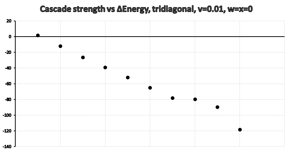
[5pt]            [5pt]

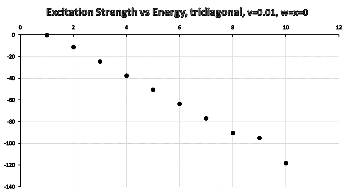
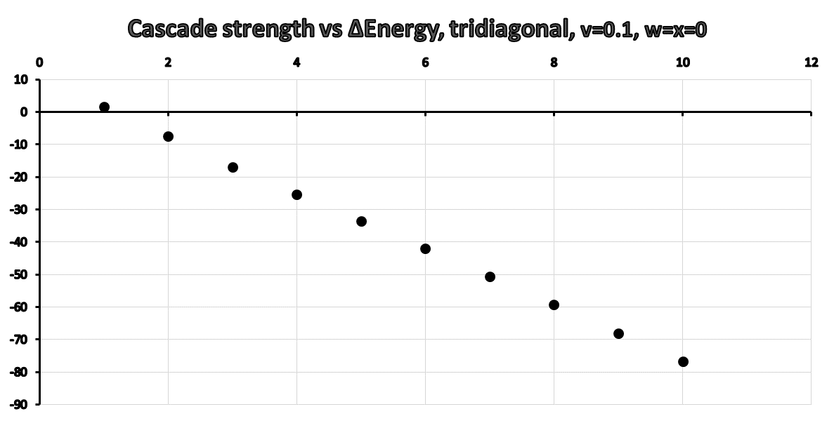
[5pt]            [5pt]

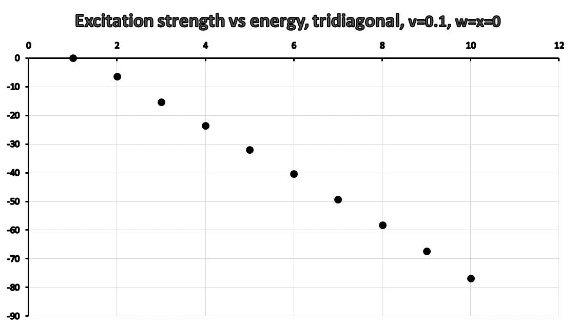
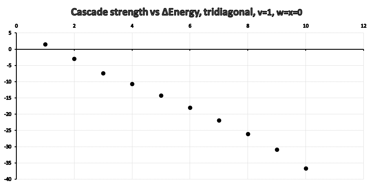
[5pt]            [5pt]

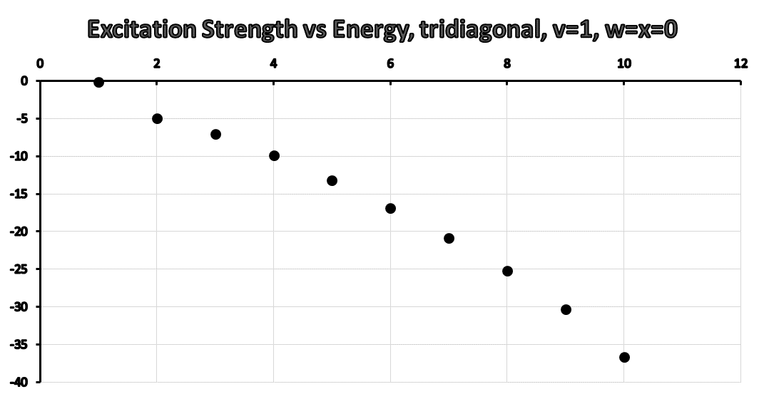
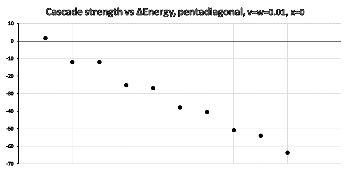
[5pt]            [5pt]

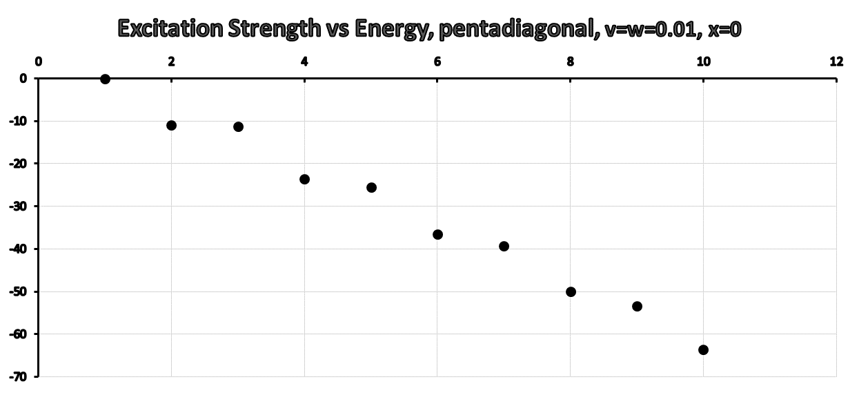
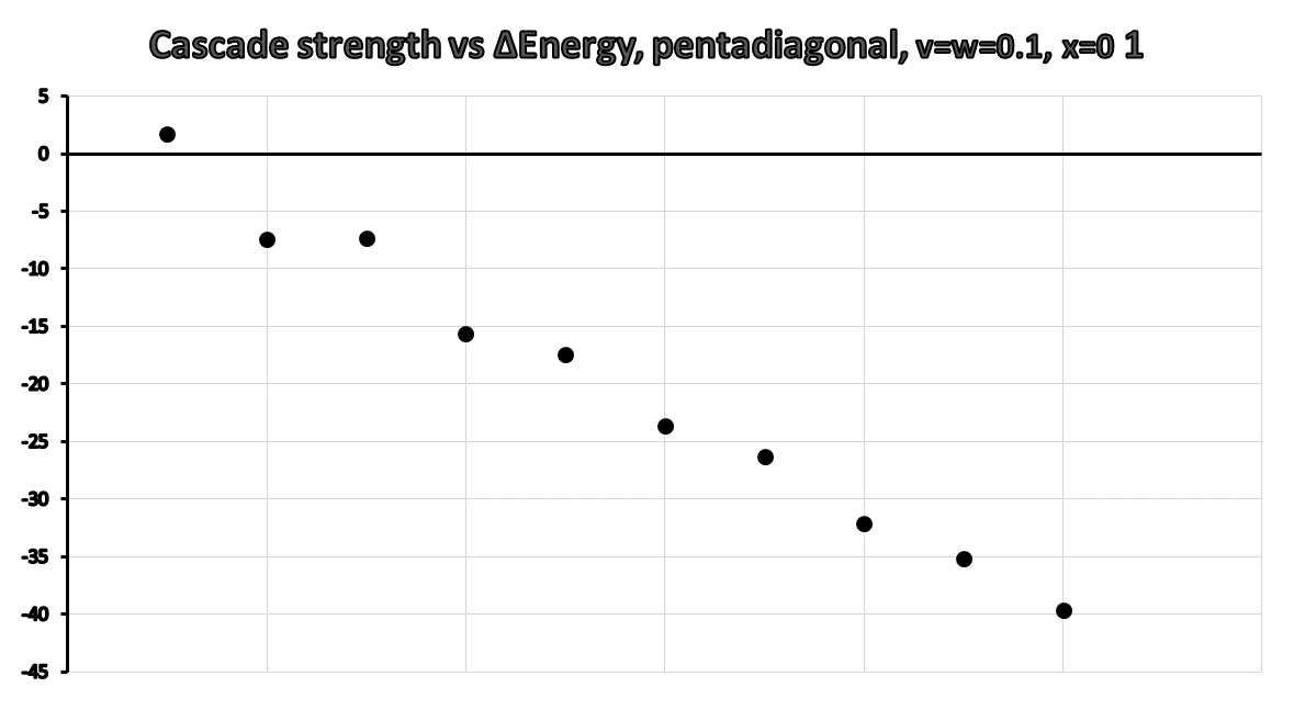
[5pt]            [5pt]

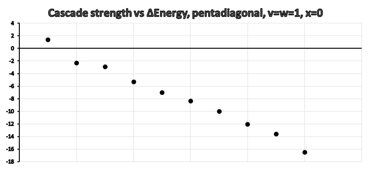
[5pt]            [5pt]

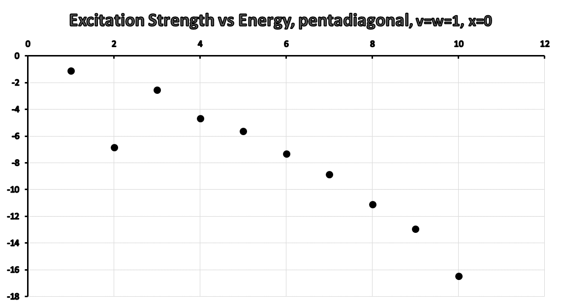
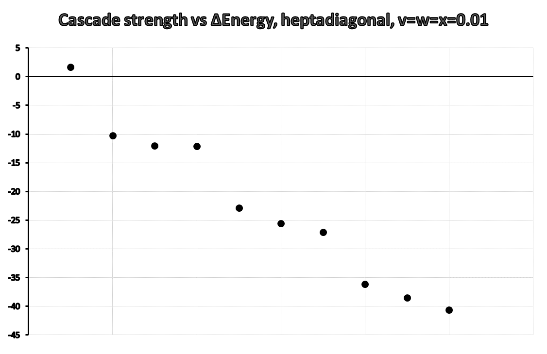
[5pt]            [5pt]

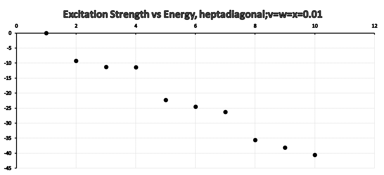
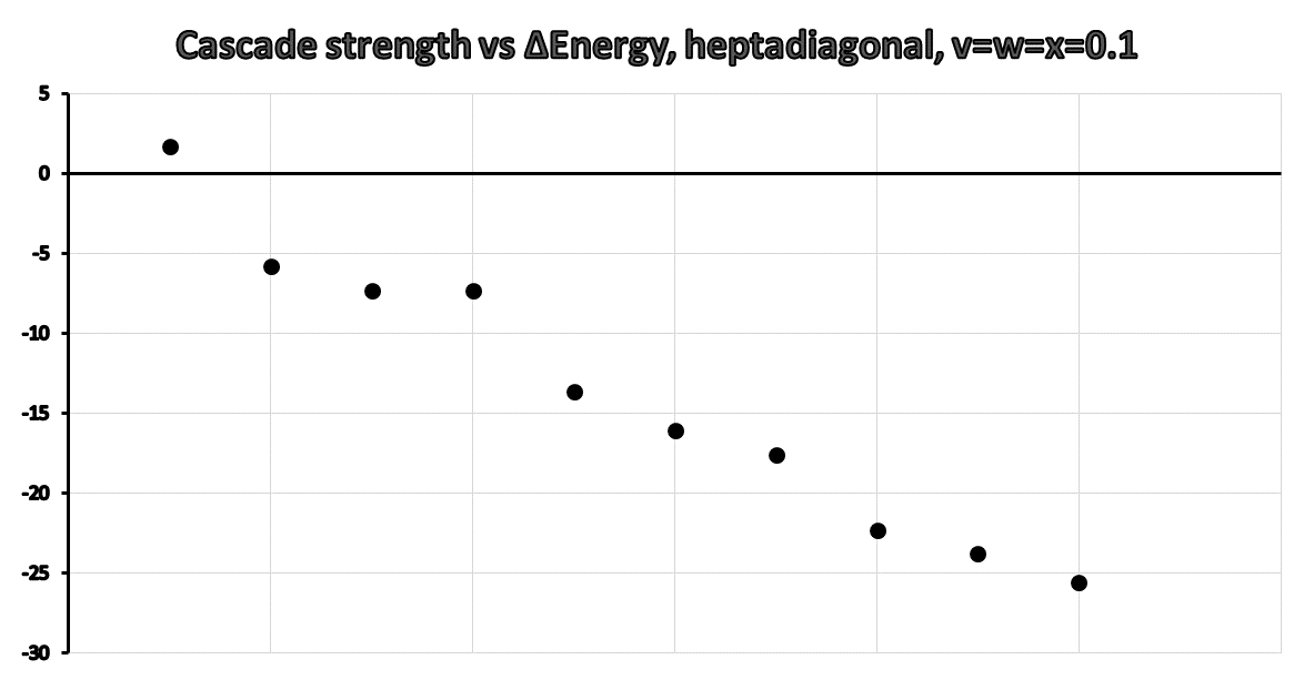
[5pt]            [5pt]

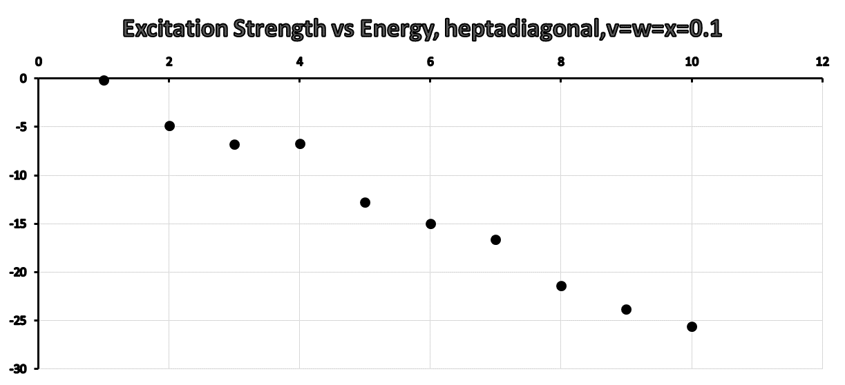
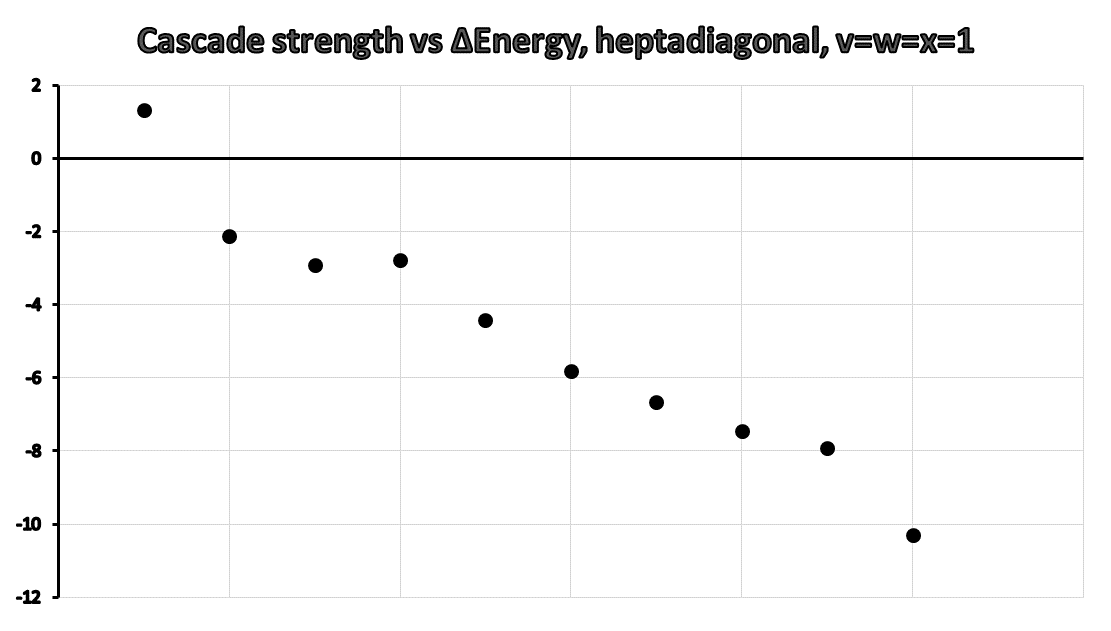
[5pt]            [5pt]

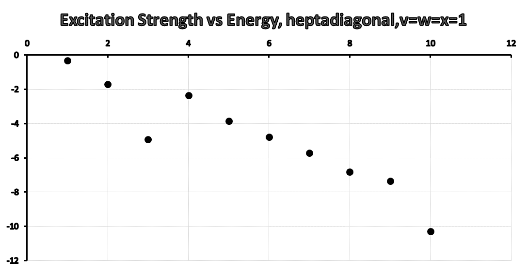
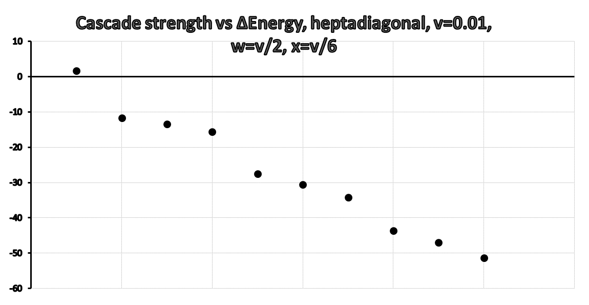
[5pt]            [5pt]

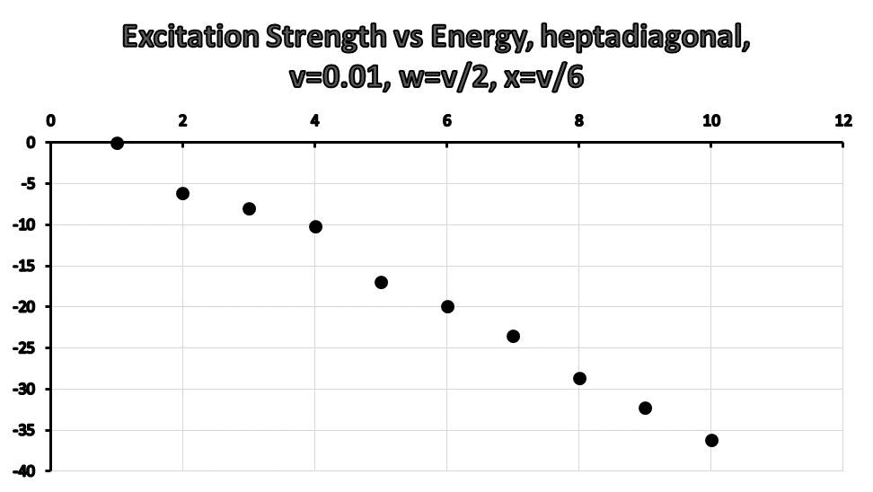
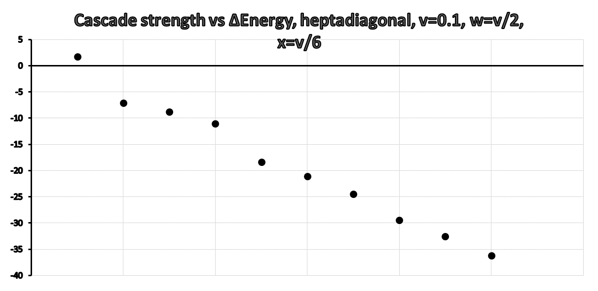
[5pt]            [5pt]

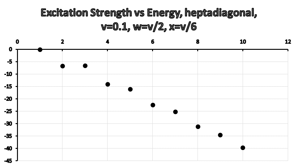
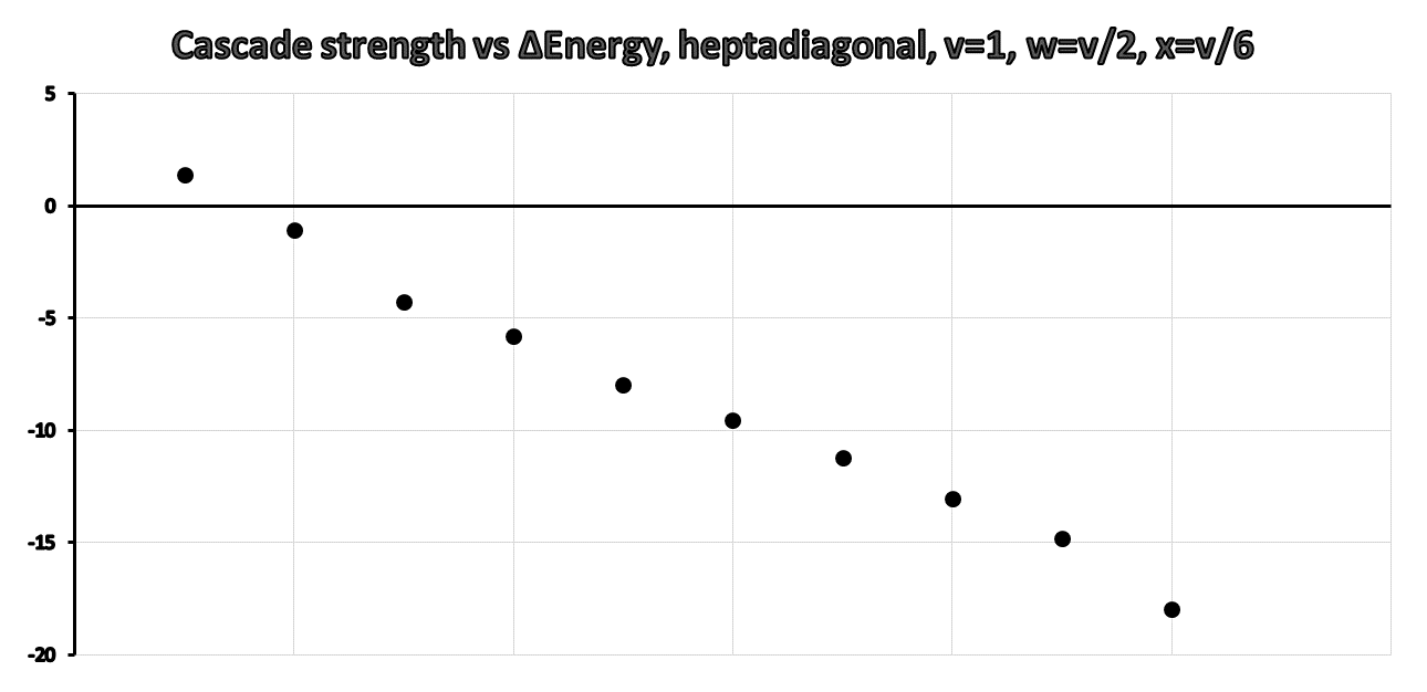
[5pt]            [5pt]

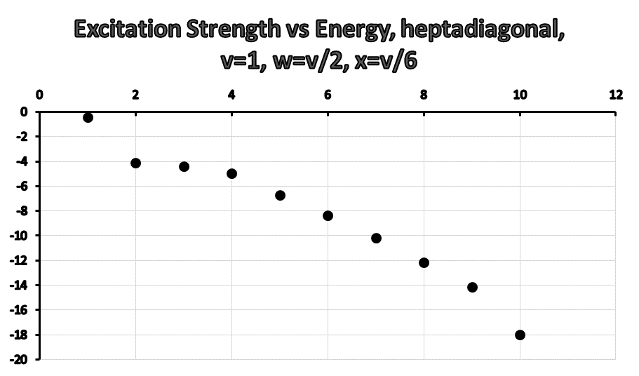
5 Discussion

We have put the cascade and excition figures side by side to make the point that , although not identical, they are remarkably similar. We emphasize that cascade is not the reverse of excitation. In the latter we always start with the lowest state and go to the n’th excited state. In cascade we have many other (reverse) transitions e.g. from the eighth excited state to the fifth one. We first consider the tridiagonal case. One gets the best linear behavior for v/E=0.1.Linearity on a log plot implies exponential behavior. For v/E=1 the curve is dominantly linear but there is a slight arch. Surprisingly for v=0.01, there is a kink at n=9. We will later see that this is not the case for asymptotically small v/E. In the pentadiagonal case for transition strength for v=1 there is a large dip at n=2- destructive interference. It is present but less pronounced in the cascade case; also present but less pronounced for smaller v/E. For the heptadiagonal transition case with v=w=x=1 we also get a pronounced dip but at n=3. In the cascade case there is linear behavior from n=4 onward but the curve flattens out for n= 4, 3, and 2 but here is then a significant rise for n=1. However when, again for the heptadiagonal case we set v=1, w=$\frac{1}{2!}$, x=$\frac{1}{3!}$ the cascade curve looks quite linear again. This is not a complete surprise because when we make w and x smaller, we go in the direction of the tridiagonal result. In Tables 2, 3 and 4 we show the excitation strengths for v=0.01, 0.1 and in tables 5, 6, and 7 the corresponding cascade averages. In contrast to the figures we here show side by side the tri,penta and hepta diagonal results for a given v.

Table 2: Excitation Spectrum for v=1

	tri	penta	hepta	hepta vwx
1	-0.17879	-1.09417	-0.3195	-0.41621
2	-4.93803	-6.83181	-1.71336	-4.11011
3	-7.07651	-2.52695	-4.92044	-4.37961
4	-9.88843	-4.66744	-2.33968	-4.94979
5	-13.1961	-5.62655	-3.85475	-6.69694
6	-16.8808	-7.32741	-4.78282	-8.36112
7	-20.8785	-8.8552	-5.72363	-10.1684
8	-25.2209	-11.1213	-6.80623	-12.1534
9	-30.338	-12.9337	-7.35953	-14.1213
10	-36.6644	-16.4684	-10.2962	-17.9763

Table 3: Excitation Spectrum for v=0.1

	tri	penta	hepta	hepta vwx
1	-0.00738	-0.14681	-0.12787	-0.14681
2	-6.41019	-6.7705	-4.84763	-6.7705
3	-15.2755	-6.55817	-6.75191	-6.55817
4	-23.5227	-14.13	-6.68711	-14.13
5	-31.8735	-16.099	-12.7848	-16.099
6	-40.4297	-22.4111	-14.9645	-22.4111
7	-49.2041	-25.2178	-16.6326	-25.2178
8	-58.1883	-31.1712	-21.4201	-31.1712
9	-67.3691	-34.5585	-23.8361	-34.5585
10	-76.7596	-39.6674	-25.5686	-39.6674

Table 4: Excitation Spectrum for v=0.01

	tri	penta	hepta	hepta vwx
1	-7.6E-05	-0.01423	-0.01404	-0.07396
2	-10.9735	-11.009	-9.24842	-6.13671
3	-24.486	-11.2124	-11.2329	-8.00813
4	-37.3515	-23.6196	-11.3943	-10.221
5	-50.3143	-25.5145	-22.2603	-16.9359
6	-63.4797	-36.5333	-24.4962	-19.9302
7	-76.8619	-39.3634	-26.2338	-23.4957
8	-90.4727	-49.9249	-35.549	-28.6644
9	-94.8711	-53.4074	-38.0957	-32.2198
10	-118.209	-63.6203	-40.5783	-36.1814

In Table 5-7 we show results for the cascade decays.

Table 5: Cascade Decays for v=1

	tri	penta	hepta	hepta vwx
1	1.475208	1.375723	1.33565	1.419713
2	-2.97858	-2.28142	-2.12546	-1.07107
3	-7.35646	-2.92052	-2.91908	-4.28074
4	-10.701	-5.31517	-2.782	-5.81003
5	-14.253	-6.98987	-4.42519	-7.94482
6	-17.9651	-8.33056	-5.80058	-9.54138
7	-21.9022	-9.99003	-6.65594	-11.2324
8	-26.0397	-12.055	-7.46434	-13.0221
9	-30.8862	-13.58	-7.90574	-14.7925
10	-36.6644	-16.4684	-10.2962	-17.9763

Table 6: Cascade Decays for v=0.1

	tri	penta	hepta	hepta vwx
1	1.700507	1.699669	1.698715	1.700062
2	-7.36563	-7.41067	-5.80332	-7.1114
3	-16.9479	-7.37501	-7.3255	-8.75926
4	-25.274	-15.6679	-7.37551	-11.0702
5	-33.555	-17.4211	-13.6674	-18.3371
6	-41.9662	-23.6271	-16.0857	-21.1241
7	-50.5406	-26.2587	-17.5985	-24.4477
8	-59.2485	-32.1169	-22.3293	-29.4771
9	-68.0405	-35.2084	-23.7897	-32.5574
10	-76.7596	-39.6674	-25.5686	-36.1814

Table 7: Cascade Decays for v=0.01

	tri	penta	hepta	hepta vwx
1	1.704704	1.704701	1.704698	1.704703
2	-11.9639	-11.969	-10.2798	-11.738
3	-26.1929	-12.0361	-12.0326	-13.491
4	-39.1037	-25.0972	-12.081	-15.6637
5	-51.9939	-26.7729	-22.833	-27.57
6	-65.0163	-37.8633	-25.5572	-30.5178
7	-78.1967	-40.4355	-27.0735	-34.2006
8	-79.6778	-50.8625	-36.0801	-43.6991
9	-89.5096	-53.9601	-38.4745	-47.0518
10	-118.209	-63.6203	-40.5783	-51.3127

6 Weak Coupling Limit for a Tridiagonal Matrix with T₂ Transition Operator

We can show that with T₂ tranistion operator <n T₂ (n+1)> = $\sqrt{n+1}$

in the weak coupling limit $u=\frac{v}{E}$ is very small

O(0 $\rightarrow$ n) has the structure $(\frac{v}{E})^{(n-1)}$ A_n where A_n does not depend on v/E.

ln (O²)= (n-1) ln($(\frac{v}{E})^{2}$) +ln (A${}_{n}^{2}$) in the weak coupling limit

Note that by making $\frac{v}{E}$ very small ln(($\frac{v}{E}$) ²) becomes very large and negative thus drowning out the term ln (A${}_{n}^{2}$). Thus we get ln($O^{2}$) approaches (n-1) ln($(\frac{v}{E})^{2}$). The fact that this ln($O^{2}$) is linear in (n-1) proves that we have exponential behavior for $O^{2}$. In a previous work [5?] we considered the weak coupling limit for the transition operator T₁. In that case O(1 $\rightarrow$ n) was of the $(\frac{v}{E})^{m}$ A(1 $\rightarrow$ n). However m was not the same as (n-1) so there was no exponential behavior for T₁. As shown in ref [5] the values of m from 1 to 9 are respectively 0, 3, 4, 5, 6, 5, 6, 7, 8. For n=10 the value of O is zero (ln($O^{2}$) = $-\infty$).

Table 8: T2 Transition Strength, $\frac{v}{E}=0.0001$

0$\rightarrow n$	ln (A${}_{n}^{2}$)	(n-1) ln ($(\frac{v}{E})^{2}$)	sum	Exact
1	0	0	0	0
2	-1.7627	-18.42	-20.1034	-20.18
3	-6.0653	-36.84	-42.9060	-42.91
4	-9.7206	-55.26	-64.9827	-64.92
5	-13.4731	-73.68	-87.1558	-87.16
6	-9.5394	-92.103	-101.6340	-101.63
7	-9.1366	-110.52	-119.6610	-119.36
8	-10.4230	–128.945	-139.368	-139.36
9	-12.6063	-147.37	-159.972	-159.97
10	-35.3138	-165.79	-201.102	-201.1

For the T₂ transition operator the expressions for A_n are given in Table 10 in terms of g_k=$\frac{1}{k!}$

Table 9: T1 Transition Strength, $\frac{v}{E}=0.0001$

n	m	ln(A${}_{n}^{2}$)	ln($\frac{v}{E}$)m	Sum	Exact
1	0	0	0	0	0
2	3	-0.8109	-55.2620	-56.07	-57.46
3	4	-4.1589	-73.6827	-77.84	-80.04
4	5	-5.9915	-92.1034	-98.09	-102.48
5	6	-8.3627	-110.5240	-118.89	-116.49
6	5	-9.5750	-92.1034	-101.67	-101.62
7	6	-9.9396	-110.5241	-120.46	-120.46
8	7	-11.6342	-128.944	-140.46	-140.58
9	8	-14.0985	-147.3654	-161.46	-161.46
10					$-\infty$

Table 10: Expressions for A_n for T₂ transition operator g_k=$\frac{1}{k!}$ .

An	expression in terms of gk
1	1
2	1-$\sqrt{2}$
3	g2-$\sqrt{2}$+g2*$\sqrt{3}$
4	g3-g2*$\sqrt{2}$+g2*$\sqrt{3}$-g3*$\sqrt{4}$
5	g4-g3*$\sqrt{2}$+g2*g2*$\sqrt{3}$-g3*$\sqrt{4}$+g4*$\sqrt{5}$
6	-g4*$\sqrt{2}$+g2*g3*($\sqrt{3}$-$\sqrt{4}$)+g4*$\sqrt{5}$-g5*$\sqrt{6}$
7	g2*g4*$\sqrt{3}$-g3*g3*$\sqrt{4}$+g4*g2*$\sqrt{5}$-g5*$\sqrt{6}$+g6*$\sqrt{7}$
8	g4*g3*($\sqrt{5}$-$\sqrt{4}$)-g2*g5*$\sqrt{6}$ +g6*$\sqrt{7}$-g7*$\sqrt{8}$
9	g4*g4*$\sqrt{5}$-g5*g3*$\sqrt{6}$+g6*g2*$\sqrt{7}$-g7*$\sqrt{8}$+g8*$\sqrt{9}$
10	g9-g8*$\sqrt{2}$+g2*g7*$\sqrt{3}$-g6*g3*$\sqrt{4}$+g4*g5*$\sqrt{5}$-g4*g5*$\sqrt{6}$+g6*g3*$\sqrt{7}$-g7*g2*$\sqrt{8}$+g8*$\sqrt{9}$-g9*$\sqrt{10}$

In the (n,$\gamma$) results the best example of a linear behavior on a log plot is given in Fig 1 of Brown and Larsen [7]. Of course the Hamiltonian they use is completely different from the simple one used here, but it suggests that the phenomenon of exponential behavior is more widespread than one might initially think. We have given support to this notion by proving that one gets exponential behavior in the weak coupling limit.

References

- [1] A.Kingan, M. Quinonez, X. Yu and L. Zamick , International Journal of Modern Physics E Vol. 28,1850090 (2018)
- [2] A.Kingan, M. Quinonez, X. Yu and L. Zamick , arXiv:nucl-th/1803.00645 (2018)
- [3] A. Kingan and L. Zamick, International Journal of Modern Physics E, Vol 26,(2018) 1850064
- [4] A.Kingan and L. Zamick ,International Journal of Modern Physics E Vol.27, NO 10 (2018) 1850087
- [5] L.Wolfe and L. Zamick, International Journal of Modern Physics E Vol. 28, No. 5 (2019) 1950037
- [6] R. Schwengner, S. Frauendorf and A. C. Larson, Phys. Rev. Lett. 111 (2013) 232504
- [7] B. Alex Brown and A.C. Larsen Phys. Rev. Lett. 113, 252502 (2014)
- [8] Siega, Phys. Rev. Lett. 119 (2017) 052502 Karampagia, B. A. Brown and V. Zelevinsky, Phys. Rev C 95 (2017) 024322
- [9] R. Schwengner, S. Frauendorf and B.A. Brown, Phys. Rev. Lett. 118 (2017) 092507
- [10] R. Schwengner, S. Frauendorf and A. C. Larson, Phys. Rev. Lett. 111 (2013) 232504 B. Alex Brown and A.C. Larsen Phys. Rev. Lett. 113, 252502 (2014)
- [11] Siega, Phys. Rev. Lett. 119 (2017) 052502 Karampagia, B. A. Brown and V. Zelevinsky, Phys. Rev C 95 (2017) 024322
- [12] R. Schwengner, S. Frauendorf and B.A. Brown, Phys. Rev. Lett. 118 (2017) 092507