Rational Motions with Generic Trajectories of Low Degree

Abstract

The trajectories of a rational motion given by a polynomial of degree $n$ in the dual quaternion model of rigid body displacements are generically of degree $2n$. In this article we study those exceptional motions whose trajectory degree is lower. An algebraic criterion for this drop of degree is existence of certain right factors, a geometric criterion involves one of two families of rulings on an invariant quadric. Our characterizations allow the systematic construction of rational motions with exceptional degree reduction and explain why the trajectory degrees of a rational motion and its inverse motion can be different.

MSC 2010: 70B10, 16S36, 14E05, 14H45, 51N15, 51N25

Keywords: rational motion, inverse motion, rational curve, dual quaternions, degree reduction, polynomial factorization, Darboux motion, Wunderlich motion

1 Introduction

Rational motions are of particular interest in modern kinematics and robotics. The rationality of the trajectories yields multiple algorithmic and numerical benefits, see e. g., [5, 11]. Rational motions are often represented by homogeneous transformation matrices of dimension four by four whose entries are rational functions. Our study is based on the dual quaternion model of $\operatorname{SE}(3)$ where rational motions appear as rational curves on the Study quadric $\mathcal{S}$ and are parameterized by certain polynomials with dual quaternion coefficients.

The degree of a rational motion is the maximal degree of a trajectory which, at the same time, is the degree of a generic trajectory. It coincides with the degree of the motion as rational curve in the matrix model but not with the degree as rational curve in the dual quaternion model. In fact, if the rational curve in the dual quaternion model is given by a polynomial of degree $n$, the motion degree is generically $2n$. However, exceptions to this relation of degrees do exist. The most famous example is probably the Darboux motion, see e. g., [1, Chapter 9, § 3] or [6]. It is represented by a polynomial $C$ of degree three in dual quaternions while its generic trajectories are of degree two.

Whenever the generic trajectory degree is less than $2n$, we speak of a degree reduction. It is well-known that a degree reduction is related to the existence of intersection points of the rational motion with a certain subspace of the Study quadric $\mathcal{S}$, the exceptional generator $\operatorname{E}$ (the projective space over the vector space of non-invertible dual quaternions), see e. g., [1, Chapter 11] for planar motions or [3] for certain line symmetric motions. The proofs of these papers easily generalize to arbitrary rational motions, c. f. our Proposition 5.

However, not all observed phenomena in this context can be explained by the number of intersection points. In particular, there are rational motions of degree $n$ that intersect $\operatorname{E}$ in $m$ points but, nonetheless, have trajectories of degree strictly less than $2n-m$. Again, an example is provided by the Darboux motion where we have $n=3$, $m=2$ but trajectories of degree $2<2n-m=4$.

A second issue has been pointed out by Jon M. Selig in private communication. It refers to the degrees of a rational motion and its inverse which is obtained by interchanging the moving and the fixed frame. It is an important and natural concept in mechanism science in situations where relative motions of links are studied. If a rational motion is given by a dual quaternion polynomial $C$, its inverse motion is given by the conjugate dual quaternion polynomial ${C}^{\ast}$ which apparently does not significantly differ from $C$ in its algebraic and geometric characteristics. In particular, the curves parameterized by $C$ and ${C}^{\ast}$ intersect the exceptional generator in the same number of points. However, there are rational motions where the trajectory degrees of $C$ and ${C}^{\ast}$ differ. An example is illustrated in Figure 1. The elliptic or Cardan motion [1, pp. 346–348] in the top row is characterized by having two non-parallel straight line trajectories. Its generic trajectories are ellipses, that is, rational curves of degree two. The inverse motion (Figure 1, bottom) is called cardioid motion in [1, pp. 348–349] but is also known as Oldham motion. Two rigidly connected lines move such that each line always passes through a fixed point. Its generic trajectories, limaçons of Pascal, are of degree four. Cardan and Oldham motion can be seen as special case of a Darboux motion and its inverse motion. In fact, also for a Darboux motion the trajectories are of degree two while the trajectories of the inverse motion are of degree four.

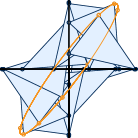
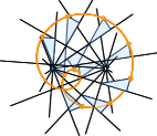
Figure 1: Cardan motion (top) and Oldham motion (bottom) are inverse but of different degrees.

There is a vague understanding in the kinematics community that an “exceptional” degree reduction can occur if intersection points of $C$ and $\operatorname{E}$ lie on a certain quadric $\mathcal{E}$ of full rank and signature zero contained in $\operatorname{E}$. However, all these geometric concepts ($\operatorname{E}$ and also $\mathcal{E}$) are invariant with respect to conjugation and thus cannot explain the difference in degree of the trajectories of $C$ and ${C}^{\ast}$.

This article will provide a comprehensive answer to the questions above. A first step in this direction was done in [10] where the authors provided a complete geometric characterization of all transformations of the seven-dimensional projective space $\mathbb{P}^{7}$ over the vector space of dual quaternions that are induced by coordinate changes in fixed and moving frame. These projective transformations not only fix the Study quadric $\mathcal{S}$, the exceptional generator $\operatorname{E}$, and the quadric $\mathcal{E}$ in $\operatorname{E}$ but also the two families of (complex) rulings on $\mathcal{E}$. Since conjugation interchanges these families, different trajectories of motion $C$ and inverse motion ${C}^{\ast}$ may be explained by the position of intersection points of $C$ with $\mathcal{E}$ with respect to one family of rulings. This turns out to be the case and is a new result for rational motions in $\operatorname{SE}(3)$. In case of the planar motion group $\operatorname{SE}(2)$, some statements on motions with algebraic trajectories and their degrees are provided in [1, Chapter 11, § 4]. They agree with the specialization of our results to planar kinematics.

We organize this paper as follows. In Section 2 we provide some basic information on quaternions and dual quaternions and their relation to kinematics. We introduce complex quaternions which are needed to properly study the quadric $\mathcal{E}$, and we explain fundamental geometric notions related to the dual quaternion parametrization of $\operatorname{SE}(3)$. Finally, we give precise definitions for concepts related to rational parametrizations, rational curves, and motion polynomials.

Our main results are proved in Section 3. We investigate in more detail the degree of trajectories and derive an algebraic criterion for exceptionally low trajectory degrees in Section 3.1. This algebraic criterion is then used for a geometric characterization in Section 3.2. We also relate our findings to some results known from literature and talk about the construction of motions with exceptionally low trajectory degree.

2 Preliminaries

In this section we collect some properties of quaternions, complex quaternions and dual quaternions and settle basic notation. We also introduce polynomials with quaternion coefficients, relate them to rational motions and study some of their fundamental properties.

2.1 Quaternions, Complex Quaternions and Dual Quaternions

The algebra of quaternions $\mathbb{H}$ is the real associative algebra generated by the base $(1,\mathbf{i},\mathbf{j},\mathbf{k})$. The non-commutative multiplication of these units is defined by

$$\mathbf{i}^{2}=\mathbf{j}^{2}=\mathbf{k}^{2}=\mathbf{i}\mathbf{j}\mathbf{k}=-1.$$

We sometimes refer to $\mathbb{H}$ as algebra of Hamiltonian quaternions in order to emphasize the distinction to the algebras of complex or dual quaternions.

The complex algebra generated by the same base and with the same rules for multiplication is denoted by $\mathbb{CH}$, elements of this algebra are called complex quaternions. A quaternion or complex quaternion $q$ is given by

$$q=q_{0}+q_{1}\mathbf{i}+q_{2}\mathbf{j}+q_{3}\mathbf{k}$$ (1)

where $q_{0}$, $q_{1}$, $q_{2}$, $q_{3}$ are real or complex coefficients, respectively. The imaginary unit of the complex numbers will be denoted by $\operatorname{i}$ and has to be distinguished from the quaternion unit $\mathbf{i}$. The (complex) quaternion conjugate is defined as ${q}^{\ast}=q_{0}-q_{1}\mathbf{i}-q_{2}\mathbf{j}-q_{3}\mathbf{k}$, the (complex) quaternion norm is $\left\|q\right\|=q{q}^{\ast}=q_{0}^{2}+q_{1}^{2}+q_{2}^{2}+q_{3}^{2}$. Note that this is not a norm in the classical sense. Whenever the norm of a (complex) quaternion $q$ is non-zero, the inverse of $q$ can be computed via ${q}^{\ast}/\left\|q\right\|$. Otherwise $q$ is a zero divisor. The only non-invertible Hamiltonian quaternion is zero whence $\mathbb{H}$ is a division ring.

The algebra of dual quaternions $\mathbb{DH}$ is obtained by extending the real coefficients in Equation (1) to dual numbers $\mathbb{D}=\mathbb{R}[\varepsilon]/\langle\varepsilon^{2}\rangle$. Any dual quaternion can be written as $p+\varepsilon d$ where $p\in\mathbb{H}$ is called the primal and $d\in\mathbb{H}$ the dual part. Multiplication follows the rules of quaternion multiplication with the additional rules $\varepsilon^{2}=0$, $\varepsilon\mathbf{i}=\mathbf{i}\varepsilon$, $\varepsilon\mathbf{j}=\mathbf{j}\varepsilon$, and $\varepsilon\mathbf{k}=\mathbf{k}\varepsilon$. The conjugation of a dual quaternion $p+\varepsilon d$ is defined by ${(p+\varepsilon d)}^{\ast}={p}^{\ast}+\varepsilon{d}^{\ast}$. The norm $\left\|p+\varepsilon d\right\|\coloneqq(p+\varepsilon d){(p+\varepsilon d)}^{\ast}=p{p}^{\ast}+\varepsilon(p{d}^{\ast}+d{p}^{\ast})$ is in general a dual number. It is real if and only if the Study condition

$$p{d}^{\ast}+d{p}^{\ast}=0$$ (2)

holds.

Quaternions, dual quaternions and complex quaternions also form a real or complex vector space. By $\mathbb{P}(\mathbb{H})$, $\mathbb{P}(\mathbb{DH})$, and $\mathbb{P}(\mathbb{CH})$ we denote the projective spaces over the respective vector space. Note that $\mathbb{P}(\mathbb{H})$ and $\mathbb{P}(\mathbb{DH})$ are real projective spaces and $\mathbb{P}(\mathbb{CH})$ is the complex extension of $\mathbb{P}(\mathbb{H})$. The elements of these projective spaces are classes of proportional non-zero vectors. The projective point represented by $q\neq 0$ is denoted by $[q]$. The symbol “$\vee$” indicates projective span. If the two points $[p]$, $[q]\in\mathbb{P}(\mathbb{CH})$ are different, their connecting line is $[p]\vee[q]$. If they are equal, we have $[p]=[q]=[p]\vee[q]$.

The Study condition (2) in the projective context is the vanishing condition of the quadratic form $p+\varepsilon d\mapsto p{d}^{\ast}+d{p}^{\ast}$. The associated bilinear form hence defines a quadric $\mathcal{S}$ in $\mathbb{P}(\mathbb{DH})$, the Study quadric, which is of great importance in spacial kinematics [12, Chapter 11].

In contrast to the quaternions $\mathbb{H}$, the complex quaternions $\mathbb{CH}$ have non-trivial zero-divisors. They are related to another important quadric. Zero divisors are precisely the zeros of the quadratic form $q\mapsto q{q}^{\ast}$ whose associated symmetric bilinear form defines a regular quadric $\mathcal{N}$ in $\mathbb{P}(\mathbb{CH})$ which we call the null quadric. It is foliated by two families of straight lines (rulings) which we call the left and the right rulings. More precisely, given $[p]\in\mathcal{N}$, the left ruling $L$ and the right ruling $R$ through $[p]$ are the point sets

$$L\coloneqq\{[q]\in\mathbb{P}(\mathbb{CH})\colon q{p}^{\ast}=0\},\quad R\coloneqq\{[q]\in\mathbb{P}(\mathbb{CH})\colon{p}^{\ast}q=0\},$$ (3)

respectively. This requires some justification which we give in the next proposition.

Proposition 1.

The sets $L$ and $R$ in (3) are two different straight lines through $[p]$ and contained in $\mathcal{N}$.

Proof.

Let $p\in\mathbb{CH}$ be a complex quaternion such that $[p]\in\mathcal{N}$, i. e., $p\neq 0$ and $\left\|p\right\|=0$, and consider the linear map

$$\varphi\colon\mathbb{CH}\to\mathbb{CH},\quad q\mapsto q{p}^{\ast}.$$

The projective space generated by the kernel of this map is precisely $L$. It obviously contains

$$p =\phantom{-}p_{0}+p_{1}\mathbf{i}+p_{2}\mathbf{j}+p_{3}\mathbf{k},$$ (4)

$$\mathbf{i}p =-p_{1}+p_{0}\mathbf{i}-p_{3}\mathbf{j}+p_{2}\mathbf{k},$$

$$\mathbf{j}p =-p_{2}+p_{3}\mathbf{i}+p_{0}\mathbf{j}-p_{1}\mathbf{k},$$

$$\mathbf{k}p =-p_{3}-p_{2}\mathbf{i}+p_{1}\mathbf{j}+p_{0}\mathbf{k}.$$

The vector space $V$ spanned by these four complex quaternions is a subspace of $\ker(\varphi)$. We will show that it is of (complex) dimension two. Assume at first that $\dim V\leq 1$. Then there exist $\alpha_{1}$, $\alpha_{2}$, $\alpha_{3}\in\mathbb{C}\backslash\{0\}$ such that $p=\alpha_{1}\mathbf{i}p=\alpha_{2}\mathbf{j}p=\alpha_{3}\mathbf{k}p$. Comparing coefficients yields the conditions

$$p_{0}=-\alpha_{i}p_{i},\quad p_{i}=\alpha_{i}p_{0}\quad\text{for $i\in\{1,2,3\}$}$$ (5)

whence $\alpha_{i}^{2}=-1$. Consequently we get $\left\|p\right\|=-2p_{0}^{2}$ and, because the norm of $p$ is assumed to be zero, it holds $p_{0}=0$. This together with Equation (5) implies that $p=0$ which is a contradiction. Thus, the kernel of $\varphi$ is at least of affine dimension two and $L$ is at least a projective line. Since the maximal subspaces on $\mathcal{N}$ are lines, it suffices to show that $L$ is contained in $\mathcal{N}$: Let $[q]\in L$ be arbitrary. We have $0=q{p}^{\ast}$. Left-multiplying both sides of this equation with ${q}^{\ast}$ yields $0=\left\|q\right\|{p}^{\ast}$. Since the norm of $q$ is a complex number and $p$ is not zero by assumption, it follows $\left\|q\right\|=0$, hence $[q]\in\mathcal{N}$.

In the same way it can be shown that $R$ is a ruling on $\mathcal{N}$. Finally, the two lines are different since the linear equations defining them are not equivalent. ∎

To conclude this subsection, we state a simple, yet important, corollary to Proposition 1 whose proof is left to the reader:

Corollary 2.

Let $[p]\in\mathcal{N}$ and $q\in\mathbb{CH}$.

1. If $qp\neq 0$ and $[qp]\neq[p]$, then $[p]$ and $[qp]$ span a left ruling of $\mathcal{N}$.

2. If $pq\neq 0$ and $[pq]\neq[p]$, then $[p]$ and $[pq]$ span a right ruling of $\mathcal{N}$.

2.2 Quaternion Polynomials and Rational Motions

For polynomials with coefficients in a ring, different notions of multiplication are conceivable. In this article, we use polynomials with coefficients from $\mathbb{H}$, $\mathbb{CH}$, or $\mathbb{DH}$ to describe rational motions. The polynomial indeterminate $t$ serves as a scalar motion parameter whence it is natural to assume that $t$ commutes with all coefficients. This defines a non-commutative multiplication of polynomials and we denote the thus obtained polynomial rings by $\mathbb{H}[t]$, $\mathbb{CH}[t]$, and $\mathbb{DH}[t]$, respectively. The conjugate ${P}^{\ast}$ of a polynomial $P$ is defined as the polynomial obtained by conjugating its coefficients. The norm polynomial is defined as $\left\|P\right\|\coloneqq P{P}^{\ast}$. It is an element of $\mathbb{R}[t]$, $\mathbb{C}[t]$ or $\mathbb{D}[t]$, respectively.

Polynomials over rings come with the notions of left/right evaluation, left/right zeros, and left/right factors. Given $P=\sum_{\ell=0}^{n}p_{\ell}t^{\ell}$ in $\mathbb{H}[t]$ (or $\mathbb{CH}[t]$, $\mathbb{DH}[t]$) we define the right evaluation of $P$ at $q\in\mathbb{H}$ (or $\mathbb{CH}$, $\mathbb{DH}$) to be $\sum_{\ell=0}^{n}p_{\ell}q^{\ell}$. The name “right evaluation” comes from the fact that the indeterminate is written to the right of the coefficients before being substituted for $q$. Quaternions where the right evaluation of a polynomial $P$ vanishes are called right zeros of $P$. The notions of “left evaluation” and “left zero” are similar but we will not need them in the following.

A polynomial $S$ is called right factor of $P$ if there exists a polynomial $F$ such that $P=FS$ and it is called a left factor if there exists a polynomial $G$ such that $P=SG$.

There is a well-known double cover of $\operatorname{SE}(3)$, the group of rigid body displacements, by the group of dual quaternions of unit norm. The dual quaternion $p+\varepsilon d$ with $\left\|p+\varepsilon d\right\|=1$ is sent to the map

$$x=x_{1}\mathbf{i}+x_{2}\mathbf{j}+x_{3}\mathbf{k}\in\mathbb{R}^{3}\mapsto px{p}^{\ast}+2p{d}^{\ast}$$ (6)

which is also the image of $-(p+\varepsilon d)$. In order to get rid of this ambiguity, we prefer a projective formulation of this homomorphism. We embed the vector space $\mathbb{R}^{4}$ into $\mathbb{H}$ via $(x_{0},x_{1},x_{2},x_{3})\hookrightarrow x_{0}+x_{1}\mathbf{i}+x_{2}\mathbf{j}+x_{3}\mathbf{k}$ and consider the real projective space $\mathbb{P}^{3}(\mathbb{R})$ over this vector space. Denote by $\mathbb{R}^{\times}$ the real multiplicative group. The factor group

$$\mathbb{DH}^{\times}\coloneqq\{p+\varepsilon d\in\mathbb{DH}\colon\left\|p+\varepsilon d\right\|\in\mathbb{R}^{\times}\}/\mathbb{R}^{\times}$$

consists of points on the Study quadric $\mathcal{S}\subset\mathbb{P}(\mathbb{DH})$ minus the exceptional generator $\operatorname{E}\subset\mathbb{P}(\mathbb{DH})$ whose points are characterized by having zero primal part $\operatorname{E}=\{[\varepsilon d]\in\mathbb{P}(\mathbb{DH})\colon d\in\mathbb{H}\}$. This yields an isomorphism from $\mathbb{DH}^{\times}$ to $\operatorname{SE}(3)$ which sends the point $[p+\varepsilon d]$ to the map

$$[x_{0}+x_{1}\mathbf{i}+x_{2}\mathbf{j}+x_{3}\mathbf{k}]\in\mathbb{P}^{3}\mapsto[p(x_{0}+x_{1}\mathbf{i}+x_{2}\mathbf{j}+x_{3}\mathbf{k}){p}^{\ast}+2x_{0}p{d}^{\ast}].$$ (7)

By projection on the primal part ($d=0$) we obtain an isomorphism between $\mathbb{P}(\mathbb{H})=(\mathbb{H}\setminus\{0\})/\mathbb{R}^{\times}$ and $\operatorname{SO}(3)$. By extension of scalars from $\mathbb{R}$ to $\mathbb{C}$ we define an action of points of $\mathbb{P}(\mathbb{CH})$ on points of complex projective three space $\mathbb{P}^{3}(\mathbb{C})$. It is precisely the zero-divisors that give singular maps of $\mathbb{P}^{3}(\mathbb{C})$.

Rational motions are obtained by replacing $p$ and $d$ in (7) with (Hamiltonian or complex) quaternion polynomials $P$ and $D$, respectively. Then the image of $[x_{0}+x]\in\mathbb{P}^{3}$ is no longer a single point but again a quaternion polynomial which we may regard as a parametric expression of a rational curve. These concepts are central for this article so that we take some care to capture all subtleties in their definitions.

Denote by $\mathbb{K}(t)$ the field of rational functions in the indeterminate $t$ over the field $\mathbb{K}$ with $\mathbb{K}=\mathbb{R}$ or $\mathbb{K}=\mathbb{C}$ and by $\mathbb{K}^{m+1}(t)$ the vector space of $(m+1)$-tuples over $\mathbb{K}(t)$. The projective space over this vector space is denoted by $\mathbb{P}^{m}(\mathbb{K}(t))$.

Definition 3.

A rational parametric expression $C$ is an element of $\mathbb{K}^{m+1}(t)$, a rational curve $[C]$ is an element of $\mathbb{P}^{m}(\mathbb{K}(t))$.

The degree $\deg C$ of a rational parametric expression $C$ is defined as the maximal degree of all coefficient functions. Given a rational curve $[C]\in\mathbb{P}^{m}(\mathbb{K}(t))$ there exists a rational parametric expression $\hat{C}$ such that $[C]=[\hat{C}]$ and the entries of $\hat{C}$ are polynomials. It is found by multiplying away the denominators of all coefficients of $C$. We will generally consider only polynomial parametric expressions. Among the many possible polynomial parametric expressions of $[C]$ the ones of minimal degree are distinguished. They are found by dividing by the greatest common divisor of all entries of $\hat{C}$ and are unique up to multiplication with a scalar. We call them reduced. The degree $\deg([C])$ of the rational curve $[C]$ is defined as degree of any reduced representation.

The value of a rational curve at a scalar $t_{0}\in\mathbb{K}$ is defined as the point $[C(t_{0})]\in\mathbb{P}^{m}(\mathbb{K})$ for any representing parametric expression where $C(t_{0})$ is well-defined an different from $0$. Note that for any $C$ there exist at most finitely many values $t_{0}\in\mathbb{K}$ that are not suitable for evaluation. Moreover, $C_{0}(t_{0})$ is always well-defined and different from zero for any reduced parametric expression $C_{0}$. Finally, we have of course $[C(t_{0})]=[\tilde{C}(t_{0})]$, whenever $[C]=[\tilde{C}]$ and these expressions are well-defined.

The Zariski closure of the point set

$$\{[C(t_{0})]\colon t_{0}\in\mathbb{K}\}$$

is an algebraic curve that, in general, contains one additional point. This point is obtained as limit of $[C(t_{0})]$ for $t_{0}\to\infty$. More precisely, we define

$$[C(\infty)]\coloneqq[\lim_{t_{0}\to\infty}t_{0}^{-n}C_{0}(t_{0})]$$

where $C_{0}$ is a reduced parametric expression and $n=\deg[C]=\deg C_{0}$. The point $[C(\infty)]$ can also be thought of as being represented by the vector of leading coefficients of $C_{0}$.

Neither the degree nor the point set obtained by evaluating at scalars or $\infty$ changes under fractional linear parameter transformation $t\mapsto(\alpha t+\beta)/(\gamma t+\delta)$ with scalars $\alpha$, $\beta$, $\gamma$ and $\delta$ that satisfy the regularity condition $\alpha\delta-\beta\gamma\neq 0$. These parameter transformations naturally include the value $t=\infty$ which is mapped to $\alpha/\gamma$ and is the pre-image of $-\delta/\gamma$ (with the conventions that $\alpha/\gamma=-\delta/\gamma=\infty$ if $\gamma=0$).

Definition 4.

The (Hamiltonian, complex or dual) quaternion polynomial $P+\varepsilon D$ is called a motion polynomial if the polynomial Study condition $P{D}^{\ast}+D{P}^{\ast}=0$ is satisfied and the norm polynomial $P{P}^{\ast}$ does not vanish.

Any motion polynomial is a rational parametric expression in the sense of Definition 3. The corresponding rational curve is called a rational motion. For Hamiltonian and complex quaternions we have $D=0$ and the Study condition in Definition 4 becomes void. Moreover, $P{P}^{\ast}\neq 0$ for all $P\in\mathbb{H}[t]\setminus\{0\}$ whence all Hamiltonian quaternion polynomials (with exception of $0$) are motion polynomials.

Evaluation of a rational motion over $\mathbb{H}$ or $\mathbb{DH}$ yields a rigid body displacement for all parameter values $t\in\mathbb{R}\cup\{\infty\}$. For any point $[x_{0}+x_{1}\mathbf{i}+x_{2}\mathbf{j}+x_{3}\mathbf{k}]=[x_{0}+x]\in\mathbb{P}^{3}$, the polynomial

$$P(x_{0}+x){P}^{\ast}+2x_{0}P{D}^{\ast}$$ (8)

is a rational parametric expression. It represents a rational curve, the trajectory of $[x_{0}+x]$ with respect to the rational motion $[P+\varepsilon D]$.

As a rational curve, any rational motion $[P+\varepsilon D]$ is equipped with the notion of a degree. But this degree is different from the usual meaning where the degree of a rational motion is defined as the maximal (and also generic) degree of any of its trajectories (c. f. [5, 11]). We adopt this latter convention. If we feel the need to distinguish between these two different concepts of degrees we speak of quaternion degree (the degree of $[P+\varepsilon D]$) and trajectory degree.

The evaluation of a motion polynomial may yield a zero divisor for finitely many parameter values $t_{0}\in\mathbb{K}\cup\{\infty\}$. It is convenient to assume that this does not happen at $t_{0}=\infty$, that is, the leading coefficient of $P+\varepsilon D$ is invertible. This is no loss of generality as we may apply a suitable fractional linear parameter transformation. Multiplying (from the left or from the right) with the inverse of the leading coefficient then yields a monic motion polynomial. This amounts to a mere change of coordinates in the moving or fixed coordinate frame of the rational motion under consideration. Once more, this is no loss of generality in our context. Hence, we will feel free to assume that a motion polynomial is monic whenever this seems appropriate.

3 Exceptionally Low Degree of Trajectories

A motion polynomial $P+\varepsilon D\in\mathbb{DH}[t]$ of degree $n$ describes a rational motion. We assume that $P+\varepsilon D$ is reduced whence also the rational motion is of quaternion degree $n$. A glance at Equation (8) confirms that its trajectories are generically of degree $2n$. But, as already mentioned in the introduction, it is possible that this degree drops. Our aim in this section is a characterization of reduced motion polynomials of degree $n$ that parameterize rational motions of trajectory degree strictly less than $2n$.

The trajectory of an arbitrary point $[x_{0}+x]\in\mathbb{P}^{3}$ with $x=x_{1}\mathbf{i}+x_{2}\mathbf{j}+x_{3}\mathbf{k}$ is given by (8). We may re-write this as

$$x_{0}\left\|P\right\|+Px{P}^{\ast}+2x_{0}P{D}^{\ast}$$ (9)

and we assume, without loss of generality, that $P+\varepsilon D$ is monic. Then the degree of the rational parametric expression (9) equals $2n$ and the degree of the corresponding rational motion is less than $2n$ precisely if the expression in Equation (9) has a real polynomial factor that is independent from $x_{0}$ and $x$. A sufficient condition for this is existence of a real polynomial factor of positive degree of the primal part $P$, i. e. $P=cQ$ with $c\in\mathbb{R}[t]$ and $Q\in\mathbb{H}[t]$. Necessity of this condition is well-known knowledge in the kinematics community but it is difficult to provide a precise reference. Given the importance for this article, we provide a proof:

Proposition 5.

The degree of the rational curve parameterized by (9) is less than $2n$ for any choice of $x_{0}$ and $x$ if and only if $P$ has a real polynomial factor of positive degree.

Proof.

We already argued for the sufficiency of this statement. In order to see necessity, assume that $\operatorname{mrpf}P=1$ (“maximal real polynomial factor”) and consider the trajectory of the special point $[x]$ (i. e. $x_{0}=0$ and $x$ is yet unspecified), given parametrically by $Px{P}^{\ast}$. Since it is a spherical curve, it is of even degree and so is its maximal real polynomial factor. Hence, we may assume that there exists a quadratic real factor of $Px{P}^{\ast}$. But then, by [7, Lemma 1], there exists a linear right factor $t-p$ of $P$ such that $t-{p}^{\ast}$ is a left factor of $x{P}^{\ast}$. Now the following hold:

• There are at most $n$ different linear right factors of $P$ [4],

• the linear polynomial $t-p$ is a right factor of $P$ if and only if $t-{p}^{\ast}$ is a left factor of ${P}^{\ast}$ (because of ${(AB)}^{\ast}={B}^{\ast}{A}^{\ast}$ for any quaternion polynomials $A$, $B\in\mathbb{H}[t]$), and

• the linear polynomial $t-{q}^{\ast}$ is a left factor of ${P}^{\ast}$ if and only if $t-x{q}^{\ast}x^{-1}$ is a left factor of $x{P}^{\ast}$.

To prove the last statement, let us at first assume that $t-{q}^{\ast}$ is a left factor of ${P}^{\ast}$, i. e. there exists $H\in\mathbb{H}[t]$ such that ${P}^{\ast}=(t-{q}^{\ast})H$. Then

$$x{P}^{\ast}=x(t-{q}^{\ast})H=(tx-x{q}^{\ast}x^{-1}x)H=(t-x{p}^{\ast}x^{-1})xH.$$

Conversely, let us assume that there exists $G\in\mathbb{H}[t]$ such that $x{P}^{\ast}=(t-x{q}^{\ast}x^{-1})G$. Then

$${P}^{\ast}=x^{-1}x{P}^{\ast}=x^{-1}(t-x{q}^{\ast}x^{-1})G=(tx^{-1}-{q}^{\ast}x^{-1})G=(t-{q}^{\ast})x^{-1}G.$$

We infer that the equation

$${p}^{\ast}=x{q}^{\ast}x^{-1}$$ (10)

must be fulfilled for two linear right factors $t-p$ and $t-q$ of $P$. However, there are only finitely many linear right factors and the solution set of (10) is of positive co-dimension. Hence, for any choice of $x$ outside the union of the solution sets of the finitely many equations of type (10) where $t-p$ and $t-q$ are right factors of $P$ ensures that the degree of $Px{P}^{\ast}$ equals $2n$. Hence, the assumption $\operatorname{mrpf}P=1$ gives a contradiction. ∎

We denote the unique monic real polynomial factor of maximal degree of $P$ by $c\coloneqq\operatorname{mrpf}P$. With this notation, the right hand side of (9) becomes

$$c(cx_{0}\left\|Q\right\|+cQx{Q}^{\ast}+2x_{0}Q{D}^{\ast}).$$

Obviously, this is a rational parametric expression of degree $2n-m$ where $m\coloneqq\deg c$. A further degree reduction occurs if and only if $c$ and $Q{D}^{\ast}$ have a common real polynomial factor of positive degree. This leads us to the following definition:

Definition 6.

Let $P+\varepsilon D\in\mathbb{DH}[t]$ be a reduced monic motion polynomial and set $c\coloneqq\operatorname{mrpf}P$. We say that a degree reduction by $m$ occurs if $c$ is of degree $m$. Denote by $Q$ the unique polynomial in $\mathbb{H}[t]$ such that $P=cQ$. We say that an exceptional degree reduction by $e$ occurs, if $c$ and $Q{D}^{\ast}$ have a real common factor of degree $e$.

To summarize, the maximal trajectory degree of a rational motion of degree $n$ with degree reduction $m$ equals $2n-m-e$ where $e$ is the degree of the real gcd of $c$ and $Q{D}^{\ast}$.

3.1 Algebraic Point of View

We continue with an alternative algebraic characterization for occurrence of an exceptional degree reduction that allows the systematic construction of rational motions with exceptionally low trajectory degree. In Section 3.2 it will be used to derive a geometric criterion.

Theorem 7.

Let $P+\varepsilon D$ be a reduced motion polynomial. Set $c\coloneqq\operatorname{mrpf}P$ and let $Q$ be such that $P=cQ$. Exceptional degree reduction occurs if and only if there exists a common right factor $H\in\mathbb{H}[t]$ of $Q$ and $D$ such that $\left\|H\right\|$ divides $c$. In this case, the degree reduces exceptionally by $\deg\left\|H\right\|$.

Proof.

By Definition 6, exceptional degree reduction occurs if $Q{D}^{\ast}$ shares a real polynomial factor of positive degree with $c$. By construction, $\gcd(c,Q)=1$. Moreover, a common real factor of $c$ and $D$ is also a real factor of $P+\varepsilon D$. But $P+\varepsilon D$ is reduced so that $\gcd(c,D)=1$ and, by [2, Proposition 2.1], a real polynomial factor $h$ of $c$ and $Q{D}^{\ast}$ exists if and only if $Q$ and $D$ have a common right factor $H$ such that $\left\|H\right\|=h$. It leads to the claimed exceptional degree reduction. ∎

Remark 8.

The degree of $\left\|H\right\|$ is even whence exceptional degree reduction occurs always by an even number.

So far, only few examples of rational motions with exceptional degree reduction appeared in literature. Among them are:

• The Cardan motion [1, Chapter 9, § 11] mentioned in Section 1 is represented by a reduced rational parametric expression of degree three but its trajectories are only of degree two.

• The same is true for the Darboux motion [1, Chapter 9, § 3]. In fact, a Darboux motion is the composition of a Cardan motion with a suitable oscillating translation.

• Rational motions with trajectories of degree three have been described by Wunderlich in [13]. Their reduced motion polynomial representation is of degree four.

Computing the quaternion degrees of these motions is an easy exercise, see e. g. [6] for the Darboux motion.

According to [13] the general form of a rational cubic motion is obtained as composition of a Darboux motion with a suitable translational motion. Our framework allows a simple re-interpretation of this result:

Example 9.

A Darboux motion can be written as $C\coloneqq\left\|Q\right\|Q+\varepsilon DQ$ with polynomials $Q$, $D\in\mathbb{H}$, $\deg Q=1$, $\deg D=2$, c. f. [6]. A linear motion polynomial $F\coloneqq f+\varepsilon G$ with $f\in\mathbb{R}[t]$ and $G\in\mathbb{H}[t]$ describes a translation. Left-multiplying $C$ with $F$ yields $W\coloneqq FC=f\left\|Q\right\|Q+\varepsilon(fD+\left\|Q\right\|G)Q$. The polynomial $W$ is of degree four so that one would expect trajectories of degree eight. But the degree of the maximal polynomial factor of its primal part equals $\deg f+\deg\left\|Q\right\|=1+2=3$ whence an ordinary degree reduction by three occurs. Moreover, the criterion of Theorem 7 ensures an exceptional degree reduction by $2\deg Q=\deg\left\|Q\right\|=2$. Thus, trajectories are indeed of degree $8-3-2=3$, as claimed by Wunderlich.

Theorem 7 allows the systematic construction of rational motions with exceptional degree reduction. Starting with a monic motion polynomial $R+\varepsilon E$, we pick an arbitrary polynomial $H\in\mathbb{H}[t]$. The rational motion $cQ+\varepsilon D$ with $c=H{H}^{\ast}$, $Q=RH$, and $D=EH$ then has an exceptional degree reduction by $2\deg H$.

An even lower degree can be obtained by choosing $H$ as a right factor of $R$, i. e. $R=R^{\prime}H$ and then considering the polynomial $cR+\varepsilon D$ or even $cR+\varepsilon FD$ where $F\in\mathbb{H}[t]$ is a polynomial only subject to the condition $\deg FD\leq\deg cR$. Note however, that $cR+\varepsilon FD$ is not generally a motion polynomial, i. e. it violates the Study condition. Thus, one has to appeal to the extension of the isomorphism (7) to a homomorphism between the group of invertible dual quaternions [8]. An alternative is, to restrict the construction to planar motions. Here $cR$ is a linear combination of $1$ and $\mathbf{k}$ and $D$ is a linear combination of $\mathbf{i}$ and $\mathbf{j}$. If $F$ is also chosen as linear combination of $1$ and $\mathbf{k}$ it is guaranteed that $cR+\varepsilon FD$ is a planar motion polynomial.

Here is a concrete example of the construction above:

Example 10.

The line with the parametric expression $t-\mathbf{k}+\varepsilon\mathbf{j}$ on the Study quadric represents a planar rotation around a fixed axis different from $\mathbf{k}$. Its primal part $P\coloneqq t-\mathbf{k}$ has the norm $c\coloneqq t^{2}+1$. Multiplying the primal part with $c$ and the dual part with $P$ from the right yields the polynomial $c(t-\mathbf{k})+\varepsilon(t\mathbf{i}+\mathbf{j})$. It parameterizes a planar motion of quaternion degree three with trajectories of degree two, hence a Cardan motion [5].

3.2 Geometrical Point of View

Now we complement the algebraic criterion of Theorem 7 for exceptional degree reduction by a geometric interpretation.

Theorem 11.

Let $P+\varepsilon D$ be a reduced motion polynomial. Set $c\coloneqq\operatorname{mrpf}P$ and let $Q$ be such that $P=cQ$. If there exists a quadratic real factor $(t-z)(t-\overline{z})$ with $z\in\mathbb{C}$ of $c$ such that $[Q(z)]$ and $[D(z)]$ lie on a left ruling of the null quadric $\mathcal{N}$ in $\mathbb{P}(\mathbb{CH})$, there is an exceptional degree reduction by two. This condition is also necessary.

Remark 12.

Note that the formulation of Theorem 11 holds for $[Q(z)]=[D(z)]$ as well. In this case, the two points lie on a left ruling but do not span it. Of course, the criterion of Theorem 11 also implies that $[Q(\overline{z})]$ and $[D(\overline{z})]$ lie on a left ruling.

Proof of Theorem 11.

We assume at first that exceptional degree reduction by two occurs. By Theorem 7, there exist polynomials $Q^{\prime}$, $D^{\prime}$, $H\in\mathbb{H}[t]$ such that $Q=Q^{\prime}H$, $D=D^{\prime}H$, $\deg H=1$ and $\left\|H\right\|$ divides $c$. Moreover, $H$ cannot be real because $Q$ has no real factors. Thus, there exists $z\in\mathbb{C}\setminus\mathbb{R}$ such that $\left\|H\right\|=(t-z)(t-\overline{z})$. But then

$$Q(z){D}^{\ast}(z)=(Q{D}^{\ast})(z)=(Q^{\prime}H{H}^{\ast}{D^{\prime}}^{\ast})(z)=(H{H}^{\ast})(z)(Q^{\prime}{D^{\prime}}^{\ast})(z)=0$$

because $(H{H}^{\ast})(z)=\left\|H\right\|(z)=0$. Note that $Q(z)$ and $D(z)$ cannot vanish (because $P+\varepsilon D$ is assumed to be reduced and $\operatorname{mrpf}Q=1$) so that $[Q(z)]$ and $[D(z)]$ are well defined points. By Proposition 1, $[Q(z)]\vee[D(z)]$ lies on a left ruling. (This includes the case $[Q(z)]=[D(z)]$.)

Now assume conversely that there exists $z\in\mathbb{C}$ such that $[Q(z)]\vee[D(z)]$ lies on a left ruling and $c^{\prime}\coloneqq(t-z)(t-\overline{z})\in\mathbb{R}[t]$ divides $c$. Proposition 1 then implies $Q(z){D}^{\ast}(z)=(Q{D}^{\ast})(z)=0$. The same holds true for the complex conjugate $\overline{z}$ whence there exists $F\in\mathbb{H}[t]$ such that $Q{D}^{\ast}=c^{\prime}F$. Thus, exceptional degree reduction in the sense of Definition 6 occurs. ∎

Remark 13.

From Definition 6 it is immediately clear that different quadratic factors $c_{\ell}\coloneqq(t-z_{\ell})(t-\overline{z_{\ell}})$ give rise to different left rulings and contribute each to an exceptional degree reduction by two.

It seems natural to interpret factors of multiplicity $\mu>1$ of $c$ that lead to an exceptional degree reduction in terms of left rulings and their “multiplicity”. This we define as intersection multiplicity of the ruled surface spanned by $Q$ and $D$ and the ruled surface of left rulings $\mathcal{L}$, both viewed as rational curves on the so called Plücker or Klein quadric [9, Section 2.1], which provides a point model for lines in three-dimensional projective space. This point model can be constructed by identifying lines with half-turns about these lines. Half-turns are represented by dual quaternions $x+\varepsilon y$ with zero scalar parts, i. e., $(x+\varepsilon y)+({x}^{\ast}+\varepsilon{y}^{\ast})=0$. Under this assumption, the Study condition $x{y}^{\ast}+y{x}^{\ast}=0$ reduces to the Plücker condition [9, Equation (2.3)] which is the defining equation of the Plücker quadric. The line spanned by points $[a]$, $[b]\in\mathbb{P}(\mathbb{CH})$ is represented by

$$a{b}^{\ast}-{a}^{\ast}b+\varepsilon({a}^{\ast}b-b{a}^{\ast}).$$ (11)

The ruled surface of left rulings $\mathcal{L}$ is given by all dual quaternions

$$x-\varepsilon x\quad\text{where}\quad x\in\mathbb{CH},\ x+{x}^{\ast}=x{x}^{\ast}=0.$$ (12)

It is a conic on the Plücker quadric. Equation (12) follows from (3) together with (11): If the points $[a]$ and $[b]$ span a left ruling $\ell$, $a{b}^{\ast}=0$ and $b{a}^{\ast}=0$ hold, whence $\ell$ is represented by $-{a}^{\ast}b+\varepsilon{a}^{\ast}b$.

Definition 14.

For a rational curve $[C]$ the $m$-th osculating space in $[C(t_{0})]$ is the projective subspace spanned by $[C(t_{0})]$, $[\frac{\mathrm{d}}{\mathrm{d}t}C(t_{0})]$, …, $[\frac{\mathrm{d}^{m}}{\mathrm{d}t^{m}}C(t_{0})]$. Two rational curves intersect with multiplicity $\mu$ in a point if their $m$-th osculating spaces at that point agree for $m=0,1,\ldots,\mu-1$.

Because $\mathcal{L}$ is a conic on the Plücker quadric, its $m$-th osculating space for $m\geq 2$ is the conic’s support plane. We denote it by $\gamma$. It is described by (12) but with the norm condition $x{x}^{\ast}=0$ removed.

Theorem 15.

Let $P+\varepsilon D$ be a reduced motion polynomial. Set $c\coloneqq\operatorname{mrpf}P$ and let $Q$ be such that $P=cQ$. If there exists a real factor $(t-z)^{\mu}(t-\overline{z})^{\mu}$ with $z\in\mathbb{C}$, $\mu\in\mathbb{N}$ of $c$ such that the ruled surface $[Q]\vee[D]$ intersects $\mathcal{L}$ in $[Q(z)]\vee[D(z)]$ with multiplicity $\mu$, there is an exceptional degree reduction by $2\mu$.

Proof.

By (11) the ruled surface $[Q]\vee[D]$ is parameterized by the polynomial

$$Q{D}^{\ast}-{Q}^{\ast}D+\varepsilon({Q}^{\ast}D-D{Q}^{\ast}).$$ (13)

It intersects $\mathcal{L}$ with multiplicity $\mu$ in $[Q(z)]\vee[D(z)]$, i. e., their $m$-th osculating spaces coincide for $m=0,1,\ldots,\mu-1$. For $\mu=1$ this means that $[Q(z)]\vee[D(z)]$ is a left ruling. For $\mu=2$ this means that in addition the first derivative point lies on the conic tangent in $[Q(z)]\vee[D(z)]$. Because ruled surfaces are curves on a common quadric (the Plücker quadric), this is equivalent to the seemingly weaker condition that the derivative point lies in the conic’s support plane $\gamma$. For $\mu\geq 3$ this means that also the higher order derivative points lie in $\gamma$. All in all, intersection with multiplicity $\mu$ happens if all derivative points up to order $\mu-1$ lie in $\gamma$.

The condition that the $m$-th derivative point at $t=z$ lies in the support plane of $\mathcal{L}$ (viewed as a conic on the Plücker quadric) is

$$\frac{\mathrm{d}^{m}}{\mathrm{d}t^{m}}(Q{D}^{\ast}-{Q}^{\ast}D)(z)+\frac{\mathrm{d}^{m}}{\mathrm{d}t^{m}}({Q}^{\ast}D-D{Q}^{\ast})(z)=0.$$

Using the Study condition $Q{D}^{\ast}+D{Q}^{\ast}=0$, it reduces to

$$\frac{\mathrm{d}^{m}}{\mathrm{d}t^{m}}(Q{D}^{\ast})(z)=0.$$

Hence, intersection with multiplicity $\mu$ implies that $(t-z)^{\mu}$ is a factor of $Q{D}^{\ast}$. The same is true for $(t-\overline{z})^{\mu}$ and, by Definition 6, exceptional degree reduction by $2\mu$ occurs. ∎

Remark 16.

From the proof of Theorem 15 it is easy to infer that an exceptional degree reduction by $2\mu$ caused by a real factor $(t-z)^{\mu}(t-\overline{z})^{\mu}$ of $c$ and $Q{D}^{\ast}$ implies intersection multiplicity $\mu$ of $\mathcal{L}$ and the ruled surface $[Q]\vee[D]$ at $[Q(z)]\vee[D(z)]$ (and also at $[Q(\overline{z})]\vee[D(\overline{z})]$). Similar to Remark 13 we can argue that common quadratic real factors of $c$ and $Q{D}^{\ast}$ and their multiplicities are in one-to-one correspondence with left rulings on $[Q]\vee[D]$ and their intersection multiplicities with $\mathcal{L}$.

The geometric characterization of exceptional degree reduction is capable of explaining the observation that motion and inverse motion need not have trajectories of the same degree. The inverse of a rational motion $[P+\varepsilon D]$ is $[{P}^{\ast}+\varepsilon{D}^{\ast}]$. This operation does not affect the degree of the motion as rational curve on the Study quadric, but it interchanges the two families of rulings on $\mathcal{N}$. Thus, it is possible that exceptional degree reduction occurs for a rational motion while it does not for its inverse motion.

Example 17.

We consider the Darboux motion $C=\left\|Q\right\|Q+\varepsilon DQ$ of Example 9 and denote the conjugate complex roots of the maximal real polynomial factor $\left\|Q\right\|$ of the primal part by $z$ and $\overline{z}$. Evaluating reduced primal part and dual part at $z$ yields points $[Q(z)]$ and $[DQ(z)]$. We have $\left\|Q\right\|(z)=0$ and hence also

$$\left\|DQ(z)\right\|=\left\|D(z)\right\|\left\|Q(z)\right\|=0.$$

This means that the points $[Q(z)]$ and $[DQ(z)]$ lie on the null quadric $\mathcal{N}$ and, by Corollary 2, also lie on a left ruling. Since dual quaternion conjugation interchanges the two families of rulings on $\mathcal{N}$, the corresponding points of the inverse motion lie on a right ruling. Exceptional degree reduction for the inverse motion occurs if and only if they also lie on a left ruling, which is only possible if they coincide, i. e. $[Q(z)]=[DQ(z)]$. Darboux motions with this property are known as vertical Darboux motions.

4 Conclusion

We gave precise algebraic and geometric criteria on rational motions with an exceptional degree reduction, thus answering a question that has been open for a while in the kinematics community. Our criteria (Theorem 7 and Theorem 11) are not invariant with respect to conjugation. This explains the phenomenon that a motion and its inverse motion can be of different trajectory degrees.

The geometric criterion for exceptional degree reduction can also be formulated for algebraic motions (algebraic curves on the Study quadric). It is obvious to conjecture that it characterizes exceptional degree reduction also in the algebraic case. If this is the case, it would also explain the possibility of different degrees of an algebraic motion and its inverse. This is a topic of future research.

References

- [1] O. Bottema and B. Roth. Theoretical Kinematics. Dover Publications, 1990.
- [2] Charles Ching-An Cheng and Takis Sakkalis. On new types of rational rotation-minimizing frame space curves. J. Symb. Comput., 74:400–407, 2016.
- [3] Marco Hamann. Line-symmetric motions with respect to reguli. Mech. Machine Theory, 46(7):960–974, 2011.
- [4] Gábor Hegedüs, Josef Schicho, and Hans-Peter Schröcker. Factorization of rational curves in the Study quadric and revolute linkages. Mech. Mach. Theory, 69(1):142–152, 2013.
- [5] Bert Jüttler. Über zwangläufige rationale Bewegungsvorgänge. Österreich. Akad. Wiss. Math.-Natur. Kl. S.-B. II, 202(1–10):117–232, 1993.
- [6] Zijia Li, Josef Schicho, and Hans-Peter Schröcker. 7R Darboux linkages by factorization of motion polynomials. In Shuo-Hung Chang, editor, Proceedings of the 14th IFToMM World Congress, 2015.
- [7] Zijia Li, Josef Schicho, and Hans-Peter Schröcker. The rational motion of minimal dual quaternion degree with prescribed trajectory. Comput. Aided Geom. Design, 41:1–9, 2016.
- [8] Martin Pfurner, Hans-Peter Schröcker, and Manfred Husty. Path planning in kinematic image space without the Study condition. In Jadran Lenarčič and Jean-Pierre Merlet, editors, Proceedings of Advances in Robot Kinematics, 2016.
- [9] Helmut Pottmann and Johannes Wallner. Computational Line Geometry. Mathematics and Visualization. Springer, 2010. 2nd printing.
- [10] Tudor-Dan Rad, Daniel F. Scharler, and Hans-Peter Schröcker. The kinematic image of RR, PR, and RP dyads. Robotica, 36(10):1477–1492, 2018.
- [11] Otto Röschel. Rational motion design – a survey. Comput. Aided Design, 30(3):169–178, 1998.
- [12] Jon M. Selig. Geometric Fundamentals of Robotics. Monographs in Computer Science. Springer, 2 edition, 2005.
- [13] Walter Wunderlich. Kubische Zwangläufe. Österreich. Akad. Wiss. Math.-Natur. Kl. S.-B. II, 193:45–68, 1984.