Piecewise Robust Barrier Tubes for
Nonlinear Hybrid Systems with Uncertainty

Abstract

Piecewise Barrier Tubes (PBT) is a new technique for flowpipe overapproximation for nonlinear systems with polynomial dynamics, which leverages a combination of barrier certificates. PBT has advantages over traditional time-step based methods in dealing with those nonlinear dynamical systems in which there is a large difference in speed between trajectories, producing an overapproximation that is time independent. However, the existing approach for PBT is not efficient due to the application of interval methods for enclosure-box computation, and it can only deal with continuous dynamical systems without uncertainty. In this paper, we extend the approach with the ability to handle both continuous and hybrid dynamical systems with uncertainty that can reside in parameters and/or noise. We also improve the efficiency of the method significantly, by avoiding the use of interval-based methods for the enclosure-box computation without loosing soundness. We have developed a C++ prototype implementing the proposed approach and we evaluate it on several benchmarks. The experiments show that our approach is more efficient and precise than other methods in the literature.

1 Introduction

Hybrid systems (HS) [21] are a suitable mathematical framework to model dynamical systems with both discrete and continuous dynamics. This formalism has been successfully adopted to design cyber-physical systems (CPS) whose behavior is characterized by an embedded software monitoring and/or controlling a physical substratum. Formal verification of HS has indeed a practical impact in engineering by assuring important safety-critical requirements at design-time.

Despite the great effort to advance the state-of-the-art, reachability analysis of HS remains one of the most challenging verification tasks. Although the problem of reachability analysis is in general undecidable [21] for HS, in the last decade several efficient and scalable semidecidable approaches have been proposed to analyse HS with linear dynamics [14, 15, 34, 39, 19].

HS with nonlinear ordinary differential equations (ODEs) remains still very challenging to solve because these ODEs do not have a closed form solution in general. One common strategy to tackle this problem is to compute an over-approximation (also called flowpipe) that contains all the possible trajectories originating from an initial set of states within a bounded-time horizon [6, 1, 11, 9, 10]. If the overapproximation does not intersect with the unsafe set of states, then the system is safe. However, if the overapproximation is too coarse, it may intersect the unsafe set of states only due to the approximation errors and then the verdict about safety may be inconclusive. Thus, one of the main problem to address is how to efficiently compute tight over-approximations of the reachable set of states for nonlinear continuous and hybrid systems.

To overcome this problem, in a recent paper [22], we have introduced the notion of Piecewise Barrier Tubes (PBT), a new flowpipe overapproximation for nonlinear systems with polynomial dynamics. The main idea of this approach is that for each segment of a flowpipe, it constructs a coarse box that is big enough to contain the segment and then it computes in the box a set of barrier functions [32, 24] which work together to form a tube surrounding the flowpipe.

PBT has advantages over traditional time-step based methods in dealing with those nonlinear dynamical systems in which there is a large difference in speed between trajectories, producing a tight over-approximation that is time independent. However, the approach in [22] cannot handle uncertainty and hybrid systems. In addition, the use of interval method for enclosure-box computation reduces its efficiency.

In this paper, we extend the approach with the ability to handle both continuous and hybrid dynamical systems with uncertainty which can reside in parameters and/or noise. We improve the efficiency of the method significantly, by avoiding the use of interval method for enclosure-box computation without loosing soundness. We have developed a C++ prototype implementing the proposed approach and we evaluate it on several benchmarks. The experiments show that our approach is more efficient and precise than other methods proposed in the literature.

The other existing techniques used to compute a bounded flowpipe are mainly based on interval method [30] or Taylor model [4]. Interval method is quite efficient even for high dimensional systems [30], but it suffers from the wrapping effect that arises due to an uncontrollable growth of the interval enclosure that accumulates overapproximation errors. The use of Taylor model is more precise because it uses a vector of polynomials plus a vector of small intervals to symbolically represent the flowpipe. However, checking the intersection with the unsafe region requires generally the use of interval method that brings back the wrapping effect. In particular, the wrapping effect can explode easily when the flowpipe segment over a time interval is stretched drastically due to a large difference in speed between individual trajectories.

Only recently, tools such as CLRT [9, 10], Flow* [6], MathSAT SMT solver [8, 7], HySAT/iSAT [12], dReach [25], C2E2 [11] and CORA [1], have made some progresses in verifying nonlinear continuous and hybrid models. Some of these tools  [7, 25, 12] are based on decision procedures that overcome the theoretical limits in nonlinear theories over the reals. The main idea is to encode the reachability problem for nonlinear systems as first-order logic formulas over the real numbers. A satisfiability modulo theories (SMT) solver implementing such procedures can return either a verdict of unsatisfiability when the unsafe region is not reached or an inconclusive verdict [25, 12] such as $\delta$-sat if the problem is satisfiable given a certain precision $\delta$ (the same problem may result unsatisfiable by increasing the precision). However, in the case of unsatisfiability these tools generally do not provide a reachable set representation that explains the verdict. Other techniques for reachability analysis of nonlinear systems include invariant generation [29, 40, 23, 36, 37], abstraction and hybridization [35, 26, 2, 31, 16, 5].

The paper is organized as follows. Section 2 presents the necessary preliminaries. Section 3 shows how to compute robust barrier certificates using linear programming, while in Section 4 we present our approach to address the reachability analysis problem of nonlinear continuous and hybrid systems with uncertainty. Section 5 provides our experimental results and we conclude in Section 6.

2 Preliminaries

In this section, we recall some concepts used throughout the paper. We first clarify some notation conventions. If not specified otherwise, we use boldface lower case letters to denote vectors, we use $\mathbb{R}$ for the real numbers field and $\mathds{N}$ for the set of natural numbers, and we consider multivariate polynomials in $\mathbb{R}[\vec{x}]$, where the components of $\vec{x}$ act as indeterminates. In addition, for all the polynomials $B(\vec{c},\vec{x})$, we denote by $\vec{c}$ the vector composed of all the $c_{i}$ and denote by $\vec{x}$ the vector composed of all the remaining variables $x_{i}$ that occur in the polynomial. We use $\mathbb{R}_{\geq 0}$ and $\mathbb{R}_{>0}$ to denote the domain of nonnegative real number and positive real number respectively. With an abuse of notation, we sometimes use $B(\vec{x})=0$ for the semialgebraic set it defines. $\partial S$ denotes the boundary of compact set $S$.

Next, we present the notation of the Lie derivative, which is widely used in the discipline of differential geometry. Let $\vec{f}:\mathbb{R}^{n}\to\mathbb{R}^{n}$ be a continuous vector field such that $\dot{x}_{i}=f_{i}(\vec{x})$ where $\dot{x}_{i}$ is the time derivative of $x_{i}(t)$.

Definition 1 (Lie derivative)

For a given polynomial $p\in\mathbb{R}[\vec{x}]$ over $\vec{x}=(x_{1},\dots,x_{n})$ and a continuous system $\dot{\vec{x}}=\vec{f}$, where $\vec{f}=(f_{1},\dots,f_{n})$, the Lie derivative of $p\in\mathbb{R}[\vec{x}]$ along $\vec{f}$ is defined as $\mathcal{L}_{\vec{f}}p=\sum_{i=1}^{n}\frac{\partial{p}}{\partial{x_{i}}}\cdot f_{i}$.

Essentially, the Lie derivative of $p$ is the time derivative of $p$, i.e., reflects the change of $p$ over time.

In this paper, we focus on semialgebraic systems with uncertainty, which is described by the following ODE.

$$\dot{\vec{x}}=\vec{f}(\vec{x}(t),\vec{u}(t))$$ (1)

where $\vec{f}$ is a vector of polynomial functions, $\vec{x}(t)$ is a solution of the system, $\vec{u}(t)$ is the vector of uncertain parameters and/or perturbation and $\vec{u}(t)$ is Lipschitz continuous. Note that we do not make a distinction between uncertain parameters and perturbation since we deal with them uniformly. Formally, semialgebraic system with uncertainty is defined as follows.

Definition 2 (Semialgebraic system with uncertainty)

A semialgebraic system with uncertainty is a $5$-tuple $\mathcal{M}\stackrel{{\scriptstyle\mbox{def}}}{{=}}\langle X,\vec{f},\mathit{X_{0}},\mathcal{I},\mathcal{U}\rangle$, where

1. $X\subseteq\mathbb{R}^{n}$ is the state space of the system $\mathcal{M}$,

2. $\vec{f}\in\mathbb{R}[\vec{x},\vec{u}]^{n}$ is locally Lipschitz continuous vector function defining the vector flow as in ODE (1),

3. $\mathit{X_{0}}\subseteq X$ is the initial set, which is semialgebraic [41],

4. $\mathcal{I}$ is the invariant or domain of the system,

5. $\mathcal{U}$ is a domain for the uncertain parameters and perturbation, i.e., $\vec{u}(t)\in\mathcal{U}$

The local Lipschitz continuity guarantees the existence and uniqueness of the differential equation $\dot{\vec{x}}=\vec{f}$ locally. A trajectory of a semialgebraic system with uncertainty is defined as follows.

Definition 3 (Trajectory)

Given a semialgebraic system with uncertainty $\mathcal{M}$, a trajectory originating from a point $\vec{x}_{0}\in\mathit{X_{0}}$ to time $T>0$ is a continuous and differentiable function $\vec{\zeta}(\vec{x}_{0},t):[0,T)\to\mathbb{R}^{n}$ such that 1) $\vec{\zeta}(x_{0},0)=\vec{x}_{0}$ 2) $\exists\vec{u}(\cdot):\forall\tau\in[0,T)$: $\frac{d\vec{\zeta}}{dt}\big{|}_{t=\tau}=\vec{f}(\vec{\zeta}(\vec{x}_{0},\tau),\vec{u}(\tau))$, where $\vec{u}(\cdot):[0,T)\rightarrow\mathcal{U}$ $T$ is assumed to be within the maximal interval of existence of the solution from $\vec{x}_{0}$.

For ease of readability, we also use $\zeta(t)$ for $\zeta(\vec{x}_{0},t)$ if it is clear from the context.

Definition 4 (Safety)

Given an unsafe set $\mathit{X_{us}}\subseteq X$, a semialgebraic system with uncertainty $\mathcal{M}$ is said to be safe if no trajectory $\vec{\zeta}(\vec{x}_{0},t)$ of $\mathcal{M}$ satisfies that $\exists\tau\in\mathbb{R}_{\geq 0}:\vec{\zeta}(\vec{x}_{0},\tau)\in\mathit{X_{us}}$, where $\vec{x}_{0}\in\mathit{X_{0}}$.

3 Robust Barrier Certificate by Linear Programming

A barrier certificate for a continuous dynamics system is a real-valued function $B(\vec{x})$ such that 1) the initial set and the unsafe set are located on different sides of the hyper-surface $\mathcal{H}=\{\vec{x}\in\mathbb{R}^{n}\mid B(\vec{x})=0\}$ respectively, and 2) no trajectory originating from the same side of $\mathcal{H}$ as the initial set can cross through $\mathcal{H}$ to reach the other side Therefore, the existence of such a function $B(\vec{x})$ can guarantee the safety of the system. The above condition can be formalized using an infinite sequence of higher order Lie derivatives [42]. Unfortunately, this formalization cannot be applied directly to barrier certificate computation. Therefore, a couple of sufficient conditions for the above condition have been proposed [24, 28, 17]. Most recently, based on the sufficient condition in [32], a new approach was proposed to overapproximate the flowpipe of nonlinear continuous dynamical systems using combination of barrier certificates [22]. However, the approach is limited to continuous dynamical systems without uncertainty. To tackle this problem, we extend the approach to deal with continuous and hybrid systems with uncertainty. Similarly, we adopt the same barrier certificate condition as [22], but we introduce the uncertainty in the barrier certificate condition. Note that in order to distinguish it from barrier certificate for dynamical system without uncertainty, we call a barrier certificate satisfying the following condition robust barrier certificate.

Theorem 3.1

Given an uncertain semialgebraic system $\mathcal{M}=\langle X,\vec{f},\mathit{X_{0}},\mathcal{I},\mathcal{U}\rangle$, let $\mathit{X_{us}}$ be the unsafe set, the system is guaranteed to be safe if there exists a real-valued function $B(\vec{x})$ such that

$$\forall\vec{x}\in\mathit{X_{0}}:B(\vec{x})>0$$ (2)

$$\forall(\vec{x},\vec{u})\in\mathcal{I}\times\mathcal{U}:\mathcal{L}_{\vec{f}}B>0$$ (3)

$$\forall\vec{x}\in\mathit{X_{us}}:B(\vec{x})<0$$ (4)

The most common approach to barrier certificate computation is by SOS programming [32, 24]. The idea of this kind of approach is to first relax the original constraints like (2)–(4) into a set of positive semidefinite (PSD) polynomials by applying Putinar representation [33], which is further relaxed by requiring every PSD polynomial has a sum-of-squares decomposition, which can be solved by SOS programming in polynomial time. However, constructing automatically a set of consistent templates for the barrier certificate as well as the auxiliary polynomials is not trivial. In addition, SOS programming method can yield fake solution sometimes due to numerical error.

An alternative to SOS programming based approaches is to use linear programming based approaches. This class of approaches relies on an LP-relaxation to the original constraint. In [38, 3], to compute Lyapunov function, an LP-relaxation was obtained by applying Handelman representation to the original constraint. Recently, this kind of LP-relaxation was adopted in [22] to compute piecewise barrier tubes. In [43], an extended version of Handelman representation, called Krivine representation [27], was employed for barrier certificate computation. Compared to Handelman representation, which can only deal with convex polytopes, Krivine representation can deal with more general compact semialgebraic sets. However, Krivine representation requires normalizing the polynomials involved, which is expensive.

In this paper, we adopt the same representation as in [22], i.e., Handelman representation as our LP-relaxation scheme for Theorem 3.1. We assume that the initial set $\mathit{X_{0}}$, the unsafe set $\mathit{X_{us}}$, the invariant $\mathcal{I}$, the parameter and/or perturbance space are all convex and compact polyhedra, i.e., $\mathit{X_{0}}=\{\vec{x}\in\mathbb{R}^{n}\mid p_{1}(\vec{x})\geq 0,\cdots,p_{m_{1}}(\vec{x})\geq 0\}$, $\mathcal{I}=\{\vec{x}\in\mathbb{R}^{n}\mid q_{1}(\vec{x})\geq 0,\cdots,q_{m_{2}}(\vec{x})\geq 0\}$, $\mathcal{U}=\{\vec{u}\in\mathbb{R}^{l}\mid w_{1}(\vec{u})\geq 0,\cdots,w_{m_{3}}(\vec{u})\geq 0\}$ and $\mathit{X_{us}}=\{\vec{x}\in\mathbb{R}^{n}\mid r_{1}(\vec{x})\geq 0,\cdots,r_{m_{4}}(\vec{x})\geq 0\}$ where $p_{i}(\vec{x})$, $q_{i}(\vec{x})$, $r_{k}(\vec{x})$ and $w_{i}(\vec{u})$, are all linear polynomials. Then, Theorem 3.1 can be relaxed as follows.

Theorem 3.2

Given a semialgebraic system with uncertainty $\mathcal{M}=\langle X,\vec{f},\mathit{X_{0}},\mathcal{I},\mathcal{U}\rangle$, let $\mathit{X_{0}}$, $\mathit{X_{us}}$, $\mathcal{I}$ and $\mathcal{U}$ be defined as above, the system is guaranteed to be safe if there exists a real-valued polynomial function $B(\vec{x})$ such that

$$B(\vec{x}) \equiv\sum_{|\vec{\alpha}|\leq M_{1}}\lambda_{\vec{\alpha}}\prod_{i=1}^{m_{1}}p_{i}^{\alpha_{i}}+\epsilon_{1}$$ (5)

$$\mathcal{L}_{\vec{f}}B \equiv\sum_{|\vec{\beta}|\leq M_{2}}\lambda_{\vec{\beta}}\prod_{i=1}^{m_{2}}q_{i}^{\beta_{i}}\prod_{j=1}^{m_{3}}w_{j}^{\beta_{m_{2}+j}}+\epsilon_{2}$$ (6)

$$-B(\vec{x}) \equiv\sum_{|\vec{\gamma}|\leq M_{3}}\lambda_{\vec{\gamma}}\prod_{i=1}^{m_{4}}r_{i}^{\gamma_{i}}+\epsilon_{3}$$ (7)

where $\vec{\alpha}=(\alpha_{k}),\vec{\beta}=(\beta_{k}),\vec{\gamma}=(\gamma_{k})$, $\lambda_{\vec{\alpha}},\lambda_{\vec{\beta}},\lambda_{\vec{\gamma}}\in\mathbb{R}_{\geq 0}$, $\epsilon_{i}\in\mathbb{R}_{>0}$ and $M_{i}\in\mathds{N},i=1,\cdots,3$.

Remark 1

Theorem 3.2 implies that the system $\mathcal{M}$ can be proved to be safe as long as we can find a real-valued polynomial function $B(\vec{x})$ such that $B(x)$, $-B(\vec{x})$ and $\mathcal{L}_{\vec{f}}B$ can be written as a nonnegative combination of the products of the powers of the polynomials defining $\mathit{X_{0}}$, $\mathit{X_{us}}$ and $\mathcal{I}\times\mathcal{U}$ respectively. This theorem provides us with a solution to solve barrier certificate by linear programming. Given a polynomial template $B(\vec{c},\vec{x})$ for $B(\vec{x})$, where $\vec{c}$ is the coefficients of the monomials to be decided in $B(\vec{c},\vec{x})$, we substitute $B(\vec{c},\vec{x})$ for $B(\vec{x})$ occurring in the conditions (5)–(7) to obtain three polynomial identities in $\mathbb{R}[\vec{x}]$ with linear polynomials in $\mathbb{R}[\vec{c},\vec{\lambda}]$ as their coefficients, where $\vec{\lambda}$ is a vector composed of all the $\lambda_{\vec{\alpha}},\lambda_{\vec{\beta}},\lambda_{\vec{\gamma}}$ occurring in (5)–(7). Since (5)–(7) are identities, then all the coefficients of the corresponding monomials on both sides of the identities must be identical. By collecting the corresponding coefficients of the monomials on both sides of the identities and let them equal respectively, we obtain a system $S$ of linear equations and inequalities on $\vec{c},\vec{\lambda}$. Now, finding a robust barrier certificate is converted to finding a feasible solution for $S$, which can be solved by linear programming efficiently. Since the degree of $B(\vec{c},\vec{x})$ is key to the expressive power of $B(\vec{c},\vec{x})$, in our implementation, we attempt to solve a barrier certificate from a group of templates with different degrees.

Due to the page limit, we do not elaborate on our algorithm for barrier certificate computation, but we demonstrate how it works in the following example.

Example 1

Given a 2D system defined by $\dot{x}=2x+3y+u_{1},\dot{y}=-4x+2y+u_{2}$, let $\mathit{X_{0}}=\{(x,y)\in\mathbb{R}^{2}\mid p_{1}=x+100\geq 0,p_{2}=-90-x\geq 0,p_{3}=y+45\geq 0,p_{4}=-40-y\geq 0\}$, $\mathcal{I}=\{(x,y)\in\mathbb{R}^{2}\mid q_{1}=x+110\geq 0,q_{2}=-80-x\geq 0,q_{3}=y+45\geq 0,q_{4}=-20-y\geq 0\}$, $\mathcal{U}=\{(u_{1},u_{2})\in\mathbb{R}^{2}\mid w_{1}=u_{1}+50.0\geq 0,w_{2}=50.0-u_{1}\geq 0,w_{3}=u_{2}+50.0\geq 0,w_{4}=50.0-u_{2}\geq 0\}$ and $\mathit{X_{us}}=\{(x,y)\in\mathbb{R}^{2}\mid r_{1}=x+98\geq 0,r_{2}=-90-x\geq 0,r_{3}=y+24\geq 0,r_{4}=-20-y\geq 0\}$. Assume $B(\vec{c},\vec{x})=c_{0}+c_{1}x+c_{2}y$, $M_{i}=\epsilon_{i}=1$ for $i=1,\cdots,3$, then we obtain the following polynomial identities according to Theorem 3.2

$$c_{1}+c_{2}x+c_{3}y-\sum_{i=1}^{4}\lambda_{1i}p_{i}-\epsilon_{1}\equiv 0$$

$$c_{2}(2x+3y+u_{1})+c_{3}(-4x+2y+u_{2})-\sum_{j=1}^{4}\lambda_{2j}q_{j}-\sum_{j=1}^{4}\lambda_{3j}w_{j}-\epsilon_{2}\equiv 0$$

$$-(c_{1}+c_{2}x+c_{3}y)-\sum_{k=1}^{4}\lambda_{4k}r_{k}-\epsilon_{3}\equiv 0$$

where $\lambda_{ij}\geq 0$ for $i,j=1,\cdots,4$. If we collect the coefficients of $x,y,u_{1},u_{2}$ in the above polynomials and let them be $0$, we obtain a system $S$ of linear polynomial equations and inequalities over $c_{i},\lambda_{ij}$. By solving $S$ using linear programming, we obtain a feasible solution with $c_{1}=-1263.5,c_{2}=-11.5,c_{3}=-5.85$.

4 Piecewise Robust Barrier Tubes

The idea of piecewise robust barrier tubes (PRBTs) is to use robust barrier tubes (RBTs) to piecewise overapproximate the flowpipe segments of nonlinear hybrid systems with uncertainty, where each RBT is essentially a cluster of robust barrier certificates which are situated around the flowpipe to form a tight tube enclosing the flowpipe. The basic idea of PRBT computation is shown in Algorithm 1.

input : $\vec{f}$: dynamics of the system; $\mathit{X_{0}}$: Initial set; $\mathcal{U}$: set of uncertainty; N: number of robust barrier tubes (RBT) in PRBT; $(\theta_{min},d_{min})$: parameters for simulation

output : PRBT: piecewise robust barrier tube

1 $\textnormal{{PRBT}}\leftarrow$ empty queue;

2 while $\textnormal{{Length}}(\textnormal{{PRBT}})<\textnormal{{N}}$ do

3       $[\textnormal{{Found}},\theta,d]\leftarrow[false,\theta_{0},d_{0}]$ ;

4       while $\theta>\theta_{min}$ do

5             $\textnormal{{E}}\leftarrow$ construct a coarse enclsoure-box for $\mathit{X_{0}}$ by $(\theta,d)$-simulation;

6             $[\textnormal{{Found}},\textnormal{{RBT}},\mathit{X_{0}}^{\prime}]\leftarrow$compute RBT inside $E$ and obtain a set $\mathit{X_{0}}^{\prime}\supseteq(\textnormal{{RBT}}\cap\partial\textnormal{{E}})$ ;

7             if not Found then

8                   $(\theta,d)\leftarrow 1/2*(\theta,d)$; // to shrink E

9                   continue;

10            else

11                   $\textnormal{{PRBT}}\leftarrow\textnormal{{Push}}(\textnormal{{PRBT}},\textnormal{{RBT}})$; // add RBT to the queue of PRBT

12                   $\mathit{X_{0}}\leftarrow\mathit{X_{0}}^{\prime}$ ; // update $\mathit{X_{0}}$ for computing next RBT

13                   break;

14            

15      if not Found then break ;

16      

17return PRBT ;

Algorithm 1 PRBT computation

4.1 Construction of the Enclosure-box

A key step in PRBT computation is the construction of enclosure-box for a given compact initial set. Note that here an enclosure-box is a hyperrectangle that entirely contains a flowpipe segment. In principle, the smaller the enclosure-box, the easier it is to compute a barrier tube. However, to make full use of the power of nonlinear overapproximation, it is desirable to have as big enclosure-box as possible so that fewer barrier tubes are needed to cover a flowpipe.

In [22], interval method was adopted to build an enclosure-box. However, the main problem with interval method is that the enclosure-box thus computed is usually very small which will result in a big number of barrier tubes for a fixed length of flowpipe. On the one hand, this will lead to an increasing burden on barrier tube computation. On the other hand, the capability of barrier tube in overapproximating complex flowpipe can not be fully released. For these reasons, we choose to use a purely simulation-based approach without losing soundness.

A key concept involved in our simulation-based enclosure-box construction is twisting of trajectory, which is a measure of maximal bending of trajectories in a box. For the convenience of presentation, we present the formal definition of twisting of trajectory as follows.

Definition 5 (Twisting of trajectory)

Let $\mathcal{M}$ be a continuous system and $\zeta(t)$ be a trajectory of $\mathcal{M}$. Then, $\zeta(t)$ is said to have a twisting of $\theta$ on the time interval $I=[T_{1},T_{2}]$, written as $\xi_{I}(\zeta)$, if it satisfies that $\xi_{I}(\zeta)=\theta$, where $\xi_{I}(\zeta)\stackrel{{\scriptstyle\text{def}}}{{=}}\sup_{t_{1},t_{2}\in I}\arccos\bigg{(}\frac{\langle\dot{\zeta}(t_{1}),\dot{\zeta}(t_{2})\rangle}{\|\dot{\zeta}(t_{1})\|\|\dot{\zeta}(t_{2})\|}\bigg{)}$.

Then, we have Algorithm 2 to compute enclosure-box.

input : $\vec{f}(\vec{x},\vec{u})$: system dynamics; $\mathit{X_{0}}$: initial set; $\mathcal{U}$: uncertain parameters; $\theta$: twisting of simulation; $\theta_{min}$: minimal theta for simulation; $d$: maximum distance of simulation;

output : E: an enclosure-box containing $\mathit{X_{0}}$; P: plane where flowpipe exits ;

G: range of intersection of $Flow_{f}(\mathit{X_{0}})$ with plane $P$ by simulation

1 $\vec{u}_{c}\leftarrow$ center point of $\mathcal{U}$;

2 $\vec{f}_{c}(\vec{x})\leftarrow$ the center dynamic $\vec{f}(\vec{x},\vec{u}_{c})$;

3 $S_{0}\leftarrow$ sample a set of points from $\mathit{X_{0}}$;

4 select a point $\vec{x}_{0}\in S_{0}$;

5 $\textnormal{{succ}}\leftarrow false$;

6 while $\theta\geq\theta_{min}$  do

7       $\vec{x}_{e}\leftarrow$ end point of $(\theta,d)$-simulation of $\vec{f}_{c}(\vec{x})$ for $\vec{x}_{0}$ ;

8       foreach $\vec{x}_{e}^{i}$: plane in the $i$’th dimension of $\vec{x}_{e}$ do

9             do simulation for all the points in $S_{0}$, update G and E ;

10             if all the simulations hit $\vec{x}_{e}^{i}$ then

11                   $\textnormal{{P}}\leftarrow\vec{x}_{e}^{i}$;

12                   $\textnormal{{succ}}\leftarrow true$;

13                  

14            

15      

16      if succ then

17             bloat E s.t $Flow_{\vec{f}}(\mathit{X_{0}})$ exits from E only through the facet in P ;

18             return $[\textnormal{{E}},\textnormal{{P}},\textnormal{{G}}]$;

19            

20      else

21             $[\theta,d]\leftarrow 1/2*[\theta,d]$;

22            

23      

24

Algorithm 2 Construct enclosure-box

Remark 2

In this paper, we assume that both $\mathit{X_{0}}$ and $\mathcal{U}$ are defined by hyperrectangles. The basic idea of enclosure-box construction is that, given a continuous dynamical system with uncertainty, we first remove the uncertainty by taking the center point $\vec{u}_{c}$ of $\mathcal{U}$ for the dynamics (line 2–2). Then, we sample a set $S_{0}$ of points from $\mathit{X_{0}}$ for simulation (line 2). Prior to doing simulation for $S_{0}$, we first select a point $\vec{x}_{0}$ (usually the center point of $\mathit{X_{0}}$) to do $(\theta,d)$-simulation to obtain the end point $\vec{x}_{e}$ of the simulation (line 2). A $(\theta,d)$-simulation is a simulation that stops either when the twisting of the simulation reaches $\theta$ or when the Euclidean distance between $\vec{x}_{0}$ and $\vec{x}_{e}$ reaches $d$. The motivation to get the end point $\vec{x}_{e}$ is that, there are $n$ planes of the form $x_{i}=\vec{x}_{e}^{i}$ (the i’th element of $\vec{x}_{e}$) intersecting at $\vec{x}_{e}$, so we want to check if one of the $n$ planes, say $P$, was hit by all the simulations that start from $S_{0}$, and if yes, it is very likely that $P$ cut through the entire flowpipe. Then, we take $P$ as one of the facets of the desired enclosure-box $\mathtt{E}$. In addition, during the simulations, we simultaneously keep updating 1) the boundary where the simulations can reach and use that range as our candidate enclosure-box $\mathtt{E}$ 2) the boundary range $\mathtt{G}$ where the simulations intersect with the plane $P:x_{i}=\vec{x}_{e}^{i}$ If we end up finding such a plane $P$, we will push the other facets of $\mathtt{E}$ outwards to make the flowpipe exit only from this specific facet of $\mathtt{E}$. Of course, this objective cannot be guaranteed only by simulation and pushing, we need to further check if the flowpipe does not intersect the other facets of $\mathtt{E}$, which can be done according to Theorem 4.1.

Theorem 4.1

Given an uncertain semialgebraic system $\mathcal{M}$ = $\langle X,\vec{f},\mathit{X_{0}},\mathcal{I},\mathcal{U}\rangle$, assume $E\subset\mathcal{I}$ is an enclosure-box of $\mathit{X_{0}}$ and $F_{i}$ is a facet of $E$. The flowpipe of $\mathcal{M}$ from $\mathit{X_{0}}$ does not intersect $F_{i}$, i.e, $(Flow_{f}(\mathit{X_{0}})\cap F_{i})\cap E=\emptyset$ if there exists a barrier certificate $B_{i}(\vec{x})$ for $F_{i}$ inside $E$.

Remark 3

Theorem 4.1 can be easily proved by the definition of barrier certificate, which is ignored here. In order to make sure that the flowpipe evades a facet $F_{i}$ of $\mathtt{E}$, according to Theorem 3.1, we only need to find a barrier certificate for $F_{i}$. In the case of no barrier certificate being found, further bloating to the facet of $E$ will be performed. If bloating facet still end up with failure, we keep shrinking $E$ by setting $(\theta,d)$ to $(\theta/2,d/2)$ until barrier certificates are found for all the facet of $E$ or $\theta$ gets less than some threshold $\theta_{min}$.

4.2 Computation of Robust Barrier Tube

An ideal application scenario of barrier certificate is when we can prove the safety property using a single barrier certificate. Unfortunately, this is usually not true because the flowpipe can be very complicated so that no polynomial function of a specified degree satisfies the constraint. In the previous subsection, we introduce how to obtain for an initial set $\mathit{X_{0}}$ an enclosure-box $E$ in which the system dynamics is simple enough so that a robust barrier certificate $B(\vec{x})$ can be easily computed. Therefore, we can compute a set of robust barrier certificates, which we call Robust Barrier Tube (RBT), to create a tight overapproximation for the flowpipe provided that there is a set of auxiliary sets serving as unsafe sets. Formally, we define RBT as follows.

Definition 6 (Robust Barrier Tube (RBT))

Given a semialgebraic system $\mathcal{M}$ = $\langle X,\vec{f},\mathit{X_{0}},\mathcal{I},\mathcal{U}\rangle$, let $E$ be an enclosure-box of $\mathit{X_{0}}$ and $X_{AS}=\{X_{AS}^{i}:X_{AS}^{i}\subseteq E\}$ be a set of auxiliary sets (AS), an RBT is a set of real-valued functions $\Phi=\{B_{i}(\vec{x}),i=1,\cdots,m\}$ such that for all $B_{i}(\vec{x})\in\Phi$: i) $\forall\vec{x}\in\mathit{X_{0}}:B_{i}(\vec{x})>0$ ii) $\forall(\vec{x},\vec{u})\in E\times\mathcal{U}:\mathcal{L}_{\vec{f}}B_{i}>0$ iii) $\forall\vec{x}\in X_{AS}^{i}:B_{i}(\vec{x})<0$

The precision of RBT depends closely on the set $X_{AS}$ of ASs. Therefore, to derive a good barrier tube, we need to first construct a set of high quality ASs. The factors that could affect the quality of the set $X_{AS}$ of ASs include 1) the number of ASs 2) the position, size and shape of AS Roughly speaking, the more ASs we have, if positioned properly, the more precise the RBT would be. Regarding the position, size and shape of AS, a desirable AS should 1) be as close to the flowpipe as possible 2) spread widely around the flowpipe 3) be shaped like a shell for the flowpipe Intuitively, a high quality set of ASs could be shaped like a ring around a human finger so that the barrier tube is tightly confined in the narrow space between the ring and the finger. With the key factors aforementioned in mind, we developed Algorithm 3 for RBT computation.

input : $\vec{f}$: system dynamics; $\mathit{X_{0}}$: Initial set; E: enclosure-box of $\mathit{X_{0}}$; $\mathcal{U}$: set of uncertainty; P: plane where flowpipe exits from enclosure-box E; G: box approx. of ($\textnormal{{P}}\cap Flow_{\vec{f}}(\mathit{X_{0}})$) by simulation; $\epsilon$: difference between AS’s (auxiliary set)

output : RBT: barrier tube; $X_{0}^{\prime}$: box over-approx. of ($\textnormal{{RBT}}\cap E$)

1

2foreach $G_{ij}$: a facet of G  do

3       AS $\longleftarrow\textnormal{{CreateAS}}(\textnormal{{G}},\textnormal{{P}},G_{ij})$;

4       while true  do

5             $[found,B_{ij}]\longleftarrow\textnormal{{ComputeRBC}}(\vec{f},\mathit{X_{0}},\textnormal{{E}},\textnormal{{AS}},\mathcal{U})$;

6            

7            if $found$ then  AS’ $\longleftarrow$ Expand (AS) ;

8             else  AS’ $\longleftarrow$ Contract (AS) ;

9            

10            if $\textnormal{{Diff}}(\textnormal{{AS}}^{\prime},\textnormal{{AS}})\leq\epsilon$ then

11                  break;

12            

13            AS $\longleftarrow$ AS’;

14            

15      

16      if $found$ then

17             $\textnormal{{RBT}}\longleftarrow\textnormal{{Push}}(\textnormal{{RBT}},B_{ij})$;

18             break;

19      else

20            return FAIL

21      

22return SUCCEED;

Algorithm 3 Compute robust barrier tube

Remark 4

In principle, the more barrier certificates we use, the better overapproximation we may achieve. However, using more barrier certificates also means more computation time. Therefore, we have to make a trade-off between precision and efficiency. In Algorithm 3, we choose to use RBT consisting of $2(n-1)$ barrier certificates for $n$ dimensional dynamical systems, which means we need to construct $2(n-1)$ ASs. We use the same scheme as in [22] to construct ASs. Recall that we get a coarse region $\mathtt{G}$ where the flowpipe intersects with one of the facets of $\mathtt{E}$ during the construction of the enclosure-box $\mathtt{E}$. Since $\mathtt{G}$ is an $n-1$ dimensional box, the RBT must contain $\mathtt{G}$. Therefore, we choose to construct $2(n-1)$ ASs which are able to form a tight hollow hyper-rectangle around $\mathtt{G}$. The idea is that for each facet $\mathtt{G}_{ij}$ of $\mathtt{G}$, we construct an $n-1$ dimensional hyper-rectangle between $\mathtt{G}_{ij}$ and $E_{ij}$ as an $\mathtt{AS}$ (line 3), where $E_{ij}$ is the $n-1$ dimensional face of $\mathtt{E}$ that corresponds to $\mathtt{G}$. Then, we use Algorithm 3 to compute an RBT(line 3). In the while loop 3, we try to find the best barrier certificate by adjusting the width of $\mathtt{AS}$ (line 3 and 3) iteratively until the difference in width between two consecutive $\mathtt{AS}$s is less than the specified threshold $\epsilon$. To be intuitive, we provide Figure 1 to demonstrate the process.

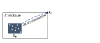
(a)

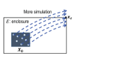
(b)

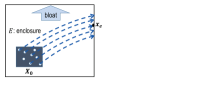
(c)

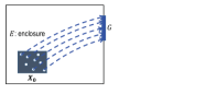
(d)

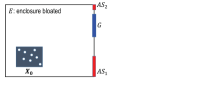
(e)

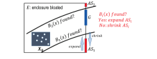
(f)

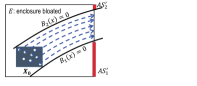
(g)

Figure 1: (a)$\rightarrow$(g): demonstration of RBT computation

4.3 PRBT for Continuous Dynamics

The idea of computing PRBT is straightforward. Given an initial set $\mathit{X_{0}}$, we first construct a coarse enclosure-box $\mathtt{E}$ containing $\mathit{X_{0}}$ and then we further compute an RBT inside $\mathtt{E}$ to get a much more precise overapproximation for the flowpipe. Meanwhile, we obtain a hyper-rectangle $R$ formed by ASs with a hollow $\mathit{X_{0}}^{\prime}$ in the middle. Since the intersection of the RBT and the facet of $\mathtt{E}$ is contained entirely in the hollow $\mathit{X_{0}}^{\prime}$ of $R$, we use $\mathit{X_{0}}^{\prime}$ as a new initial set and repeat the entire process to compute a PRBT step by step. Since our approach is time independent, the length of a PRBT cannot be measured by the length of time horizon. Hence, in our implementation, we try to compute a specified number of RBTs.

4.4 PRBT for Hybrid Dynamics

To extend our approach with the ability to deal with hybrid systems, we need to handle two problems i) compute the intersection of RBT and guard set ii) compute the image of the intersection after discrete jump In general, these two issues can be very hard depending on what kind of guard sets and transitions are defined for the hybrid systems.

In this paper, we make some assumptions on the hybrid systems under consideration. Let a discrete transition $\tau$ be defined as follows.

$$\tau_{ll^{\prime}}=\langle\mathtt{Guard}_{ll^{\prime}},\mathtt{Trans}_{ll^{\prime}}\rangle$$ (8)

where $l$ and $l^{\prime}$ are the locations of the dynamics before and after a discrete transition respectively, $\mathtt{Guard}_{ll^{\prime}}=\{\vec{x}\in\mathbb{R}^{n}\mid x_{i}\sim b_{i},\sim\in\{\leq,\geq\}\}$ and $\mathtt{Trans}_{ll^{\prime}}:\vec{x}^{\prime}=A\vec{x}$, where $A$ is an $n$-dimensional matrix. Based on this assumption, the problem of computing the intersection of RBT and guard set is reduced to computing the intersection of RBT with a plane of $x_{i}=b_{i}$, which can be handled using a similar strategy to computing the intersection of RBT with the facet of enclosure-box. Hence, we have Algorithm 4 to deal with discrete transition of a hybrid system.

input : $X_{0}^{l}$: intermediate initial set at location $l$; $\textnormal{{Guard}}_{ll^{\prime}}$: guard set of transition $\tau_{ll^{\prime}}$; $\textnormal{{Trans}}_{ll^{\prime}}$: image mapping of transition $\tau_{ll^{\prime}}$

output : $X_{0}^{l^{\prime}}$: image of transition $\tau_{ll^{\prime}}$

1 $\textnormal{{InitQ}}\leftarrow\textnormal{{Push}}(\textnormal{{InitQ}},X_{0}^{l})$;

2 while InitQ not empty  do

3       $X_{0}^{l}\leftarrow\textnormal{{Pop}}(\textnormal{{InitQ}})$;

4       $\textnormal{{E}}\leftarrow$ construct enclosure-box for $X_{0}^{l}$ ;

5       if $\textnormal{{E}}\cap\textnormal{{Guard}}_{ll^{\prime}}==\emptyset$ then

6            continue;

7      $\textnormal{{E}}\leftarrow\textnormal{{E}}\cap\overline{\textnormal{{Guard}}}_{ll^{\prime}}$;

8       $X_{\Phi\cap\textnormal{{E}}}\leftarrow$ do simulation and barrier certificate computation to find an overapproximation for the region where the flowpipe $\Phi$ intersects with the guard plane $x_{i}=b_{i}$;

9       $Q_{\Phi\cap\textnormal{{E}}}\leftarrow\textnormal{{Push}}(Q_{\Phi\cap\textnormal{{E}}},X_{\Phi\cap\textnormal{{E}}})$;

10       foreach $\textnormal{{E}}_{ij}$: facet of E except guard plane do

11             $X_{0}^{ij}\leftarrow$ do simulation and barrier certificate computation to an overapproximation for the region where the barrier tube intersects with $E_{ij}$; $\textnormal{{InitQ}}\leftarrow\textnormal{{Push}}(\textnormal{{InitQ}},X_{0}^{ij})$ ;

12            

13      

14

15$X_{\Phi\cap\textnormal{{E}}}\leftarrow$ box overapprox. $Q_{\Phi\cap E}$;

16 $X_{0}^{l^{\prime}}\leftarrow\textnormal{{Trans}}_{ll^{\prime}}X_{\Phi\cap\textnormal{{E}}}$ ;

17

Algorithm 4 handle discrete transition of hybrid system

Remark 5

The strategy to deal with discrete transitions of hybrid systems is that every time we obtain an enclosure-box $\mathtt{E}$, we first detect whether $\mathtt{E}$ intersects with some guard set $\mathtt{Guard_{ll^{\prime}}}$. If no, we proceed with the normal process of PRBT computation. Otherwise, we switch to the procedure of Algorithm 4 in which the input $X_{0}^{l}$ is the last state set whose enclosure-box intersects with $\mathtt{Guard_{ll^{\prime}}}$. Since the flowpipe may not cross through the guard plane entirely, we use the while loop in line 4 to compute an overapproximation for the intersection. The basic idea of the while loop is that, given a state set $X_{0}^{l}$, we first construct an enclosure-box $\mathtt{E}$ by simulation(line 4), if $\mathtt{E}$ intersects with $\mathtt{Guard_{ll^{\prime}}}$, we shrink $\mathtt{E}$ by cutting off the part of $\mathtt{E}$ that lies in the guard set (line 4). As a result of this operation, the flowpipe could exit from $\mathtt{E}$ not only through the guard plane but also through other facets of $\mathtt{E}$. For each of those facets, we compute an overapproximation for its intersection with the flowpipe using simulation and barrier certificate computation(line 4 and 4). In addition, since those intersections $X_{0}^{ij}$ that do not lie in the guard plane could still reach the guard plane later, we therefore push them into a queue for further exploration.

5 Implementation and Experiments

We have developed PRBT, a software prototype written in C++ that implements the concepts and the algorithms presented in this paper. PRBT computes piecewise robust barrier tubes for nonlinear continuous and hybrid systems with polynomial dynamics. We compare our approach in efficiency and precision with the state-of-the-art tools Flow* and CORA using several benchmarks of nonlinear continuous and hybrid systems. Note that since C2E2 does not support uncertainty, so we cannot compare with it. The experiments were carried out on a desktop computer with a $3.6$GHz Intel 8 Core i7-7700 CPU and $32$ GB memory.

5.1 Nonlinear Continuous Systems

We consider six nonlinear benchmark systems with polynomial dynamics for which their models and settings are provided in Table 1.

Table 1: Continuous dynamical model definitions

Model	Dynamics	Uncertainty	$\mathit{X_{0}}$
Controller 2D	$\dot{x}=d_{1}xy+y^{3}+2$	$d_{1}\in[0.95,1.05]$	$x\in[29.9,30.1]$
	$\dot{y}=d_{2}x^{2}+2x-3y\qquad$	$d_{2}\in[0.95,1.05]$	$y\in[-38,-36]$
Van der Pol	$\dot{x}=y+d_{1}$	$d_{1}\in[-0.01,0.01]$	$x\in[1,1.5]$
Oscillator	$\dot{y}=y-x-x^{2}y+d_{2}$	$d_{2}\in[-0.01,0.01]$	$y\in[2.40,2.45]$
Lotka-Volterra	$\dot{x}=x(1.5-y)+d_{1}$	$d_{1}\in[-0.01,0.01]$	$x\in[4.6,5.5]$
	$\dot{y}=-y(3-x)-d_{2}$	$d_{2}\in[-0.01,0.01]$	$y\in[1.6,1.7]$
Buckling	$\dot{x}=y+d_{1}$	$d_{1}\in[-0.01,0.01]$	$x\in[-0.5,-0.4]$
Column	$\dot{y}=2x-x^{3}-0.2y+0.1+d_{2}$	$d_{1}\in[-0.01,0.01]$	$y\in[-0.5,-0.4]$
Jet Engine	$\dot{x}=-y-1.5x^{2}-0.5x^{3}-0.5$	$d_{1}\in[-0.005,0.005]$	$x\in[1.19,1.21]$
	$\qquad+d_{1}$	$d_{2}\in[-0.005,0.005]$	$y\in[0.8,1.0]$
	$\dot{y}=3x-y+d_{2}$
	$\dot{x}=10(y-x)+d_{1}$	$d_{1}\in[-0.001,0.001]$	$x\in[1.79,1.81]$
Controller 3D	$\dot{y}=x^{3}+d_{2}$	$d_{2}\in[-0.001,0.001]$	$y\in[1.0,1.1]$
	$\dot{z}=xy-2.667z$		$z\in[0.5,0.6]$

The experimental results are reported in Table 2. Since our approach is time independent, which is different from Flow* and CORA, to make the comparison fair enough, we choose to compute a slightly longer flowpipe than the other two tools. Note that there are two columns for time for Flow*. The reason why we have an extra time column for Flow* is that it can be very fast and precise to compute the Taylor model for a given system. However, Taylor models cannot be in general applied directly to solve the safety verification problem. Checking their intersection with the unsafe set requires their transformation into simpler geometric form (e.g. box), which has an exponential complexity in the number of the dimensions and it needs to be considered in the overall running time.

Table 2: Experimental results for benchmark systems. #var: number of variables; T: computing time for flowpipe; TT: computing time including box transformation; N: number of flowpipe segments; D: candidate degrees for template polynomial (for PRBT only); TH: time horizon for flowpipe (for Flow* and CORA only). F/E: failed to terminate under 30min or exception happened.

		PRBT				Flow*			CORA
Model	#var	T	N	D	TH	T	TT	N	T	N
Controller 2D	2	35.73	12	3	0.012	48.8	417.64	240	F	1200
Van der Pol	2	221.62	17	4	6.74	23.88	1111.05	135	E	–
Lotka-Volterra	2	30.10	9	4	3.20	6.06	405.32	320	40.30	160
Buckling Column	2	74.02	35	3	14.00	F	–	–	734.81	1400
Jet Engine	2	240.98	18	4	9.50	F	–	–	1.69	190
Controller 3D	3	774.58	20	3	0.55	F	–	–	F	–

Remark 6

Table 2 shows us how brutal the reality of reachability analysis of nonlinear systems is and this gets even worse in the presence of uncertainty and large initial set. As can be seen in Table 2, both Flow* and CORA failed to give a solution for half of the benchmarks either due to timeout or due to exception. This phenomenon may be alleviated if smaller initial sets are provided or uncertainty is removed. In terms of computing time $T$, PRBT does not always outperform the other two tools. Actually, Flow* or CORA can be much faster in some cases. However, when the box transformation time for Taylor model was taken into account, the total computing time $TT$ of Flow* increased significantly. One point to note here is that, PRBT, in general, produces a much smaller number $N$ of flowpipe segments than the other two, which means that the time used to check the intersection of flowpipe with the unsafe set can be reduced considerably. In addition, as shown in Figure 2–4, PRBT is more precise than the other two on average.

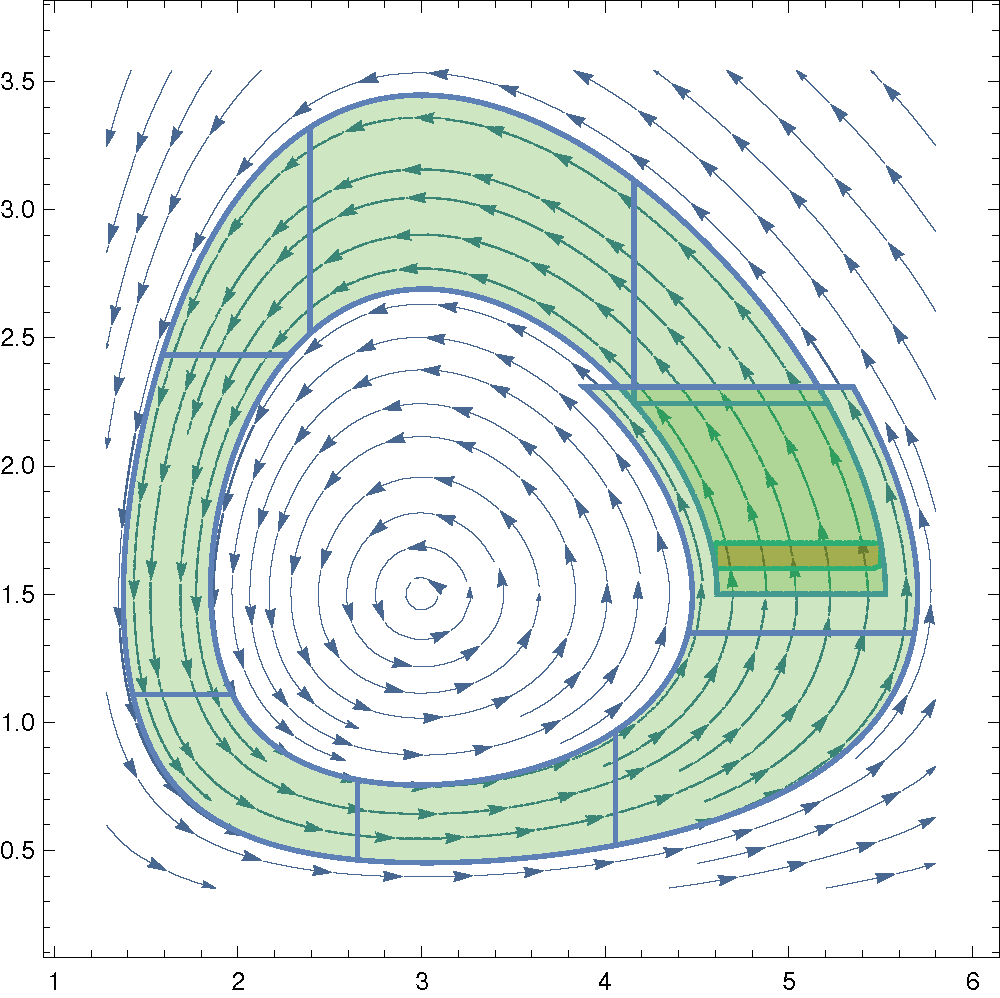
(a) PRBT

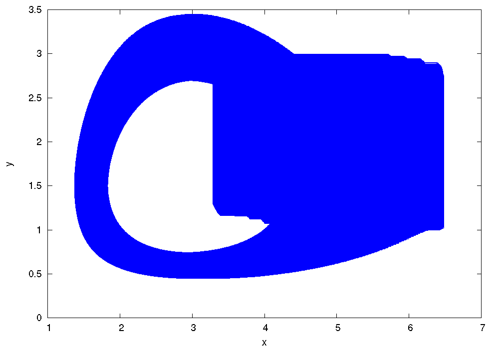
(b) Flow*

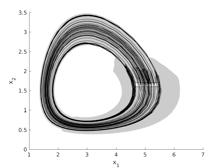
(c) CORA

(d) PRBT

Figure 2: Lotka-Volterra: (a), (b), (c); controller 3D: (d)

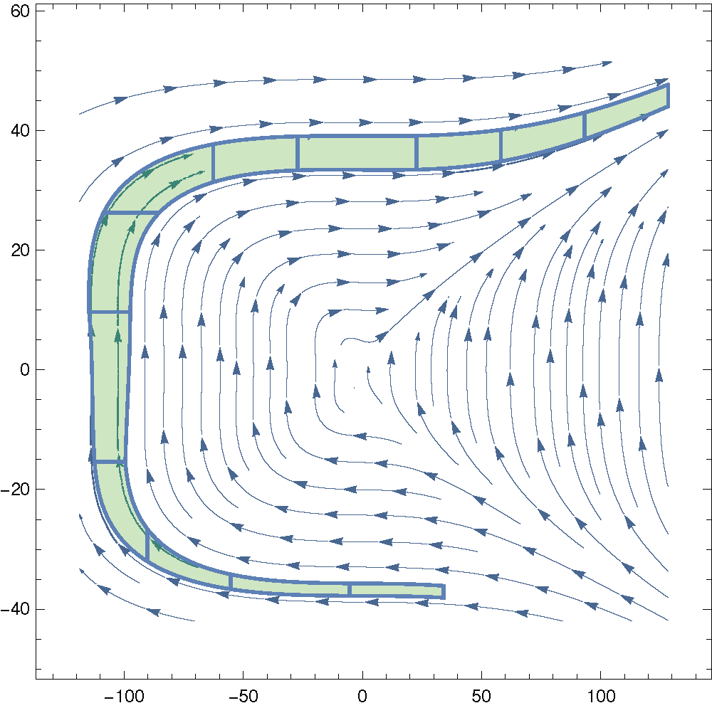
(a) PRBT

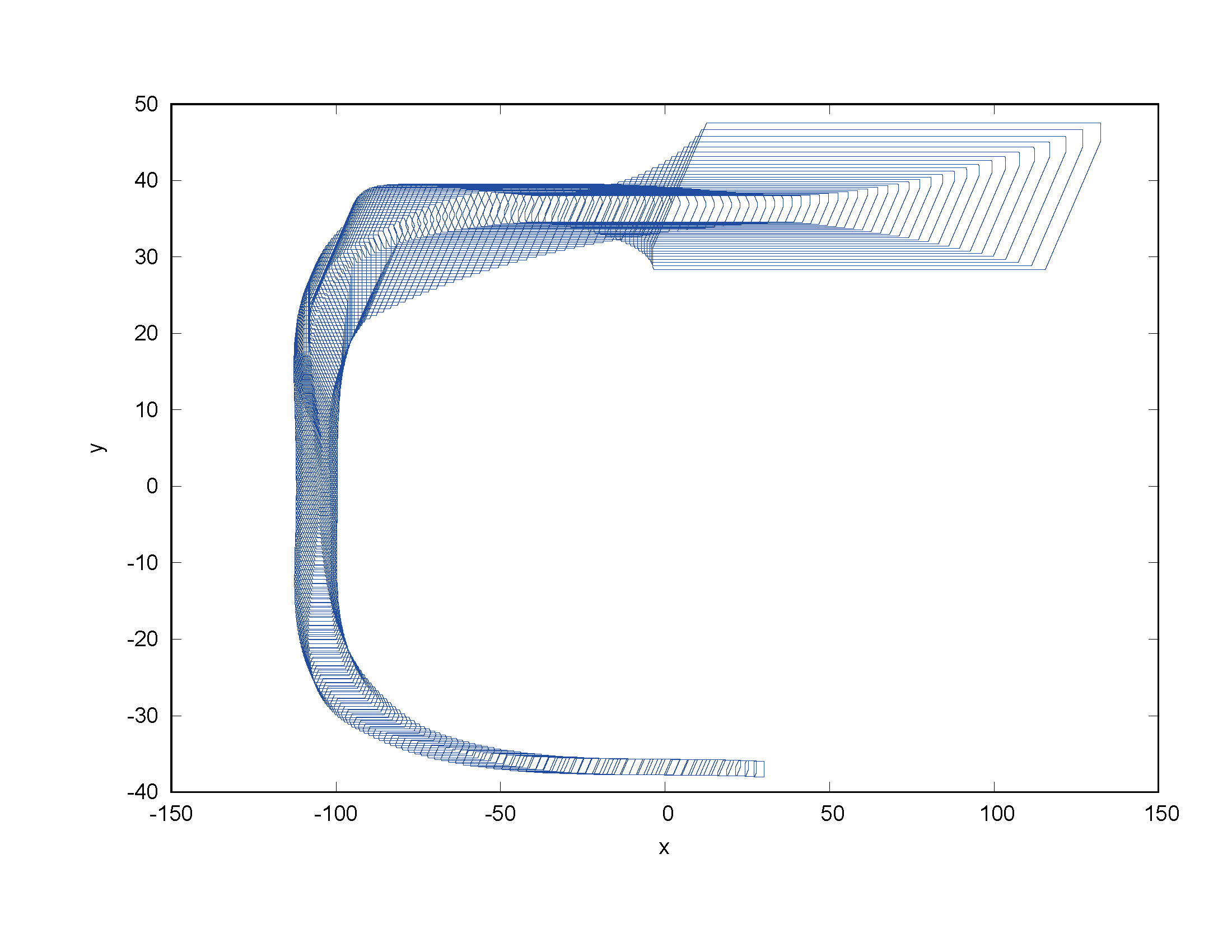
(b) Flow*

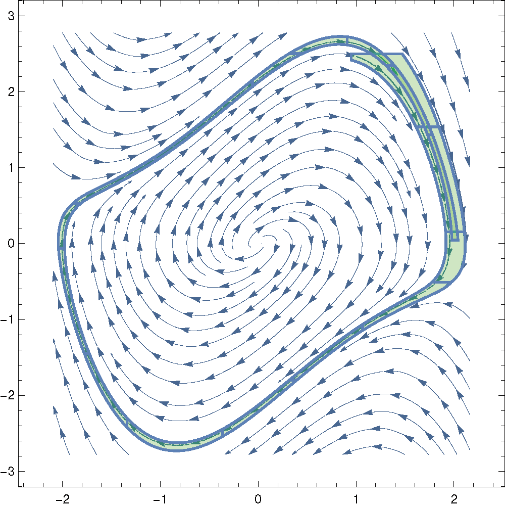
(c) PRBT

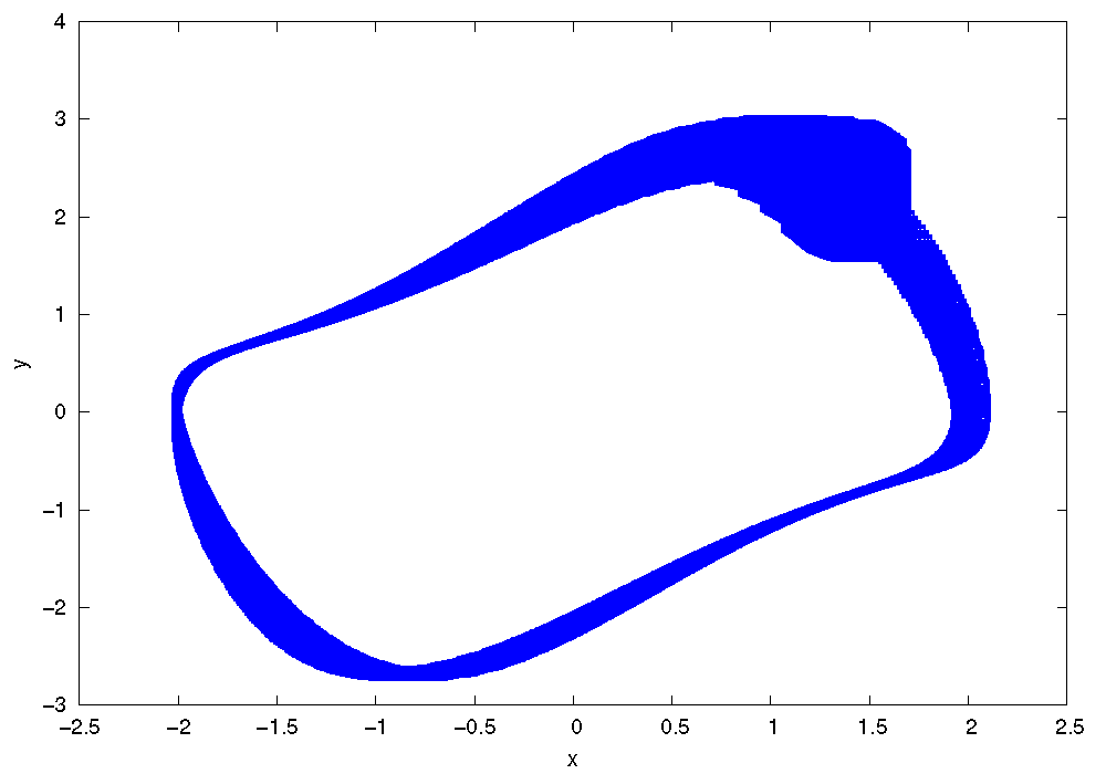
(d) Flow*

Figure 3: Controller 2d: (a), (b); Van der Pol Oscillator: (c), (d)

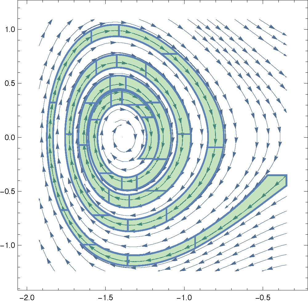
(a) PRBT

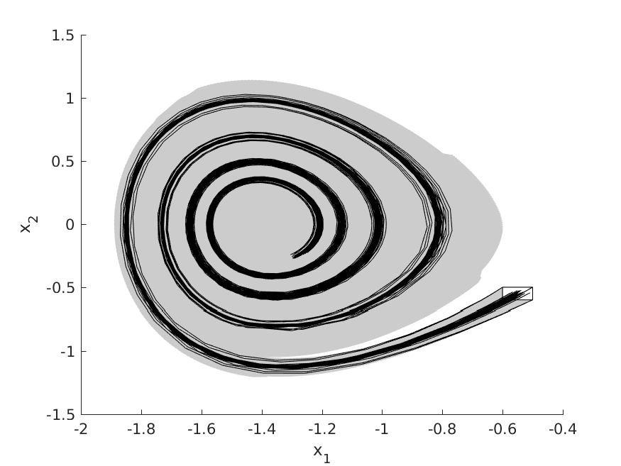
(b) CORA

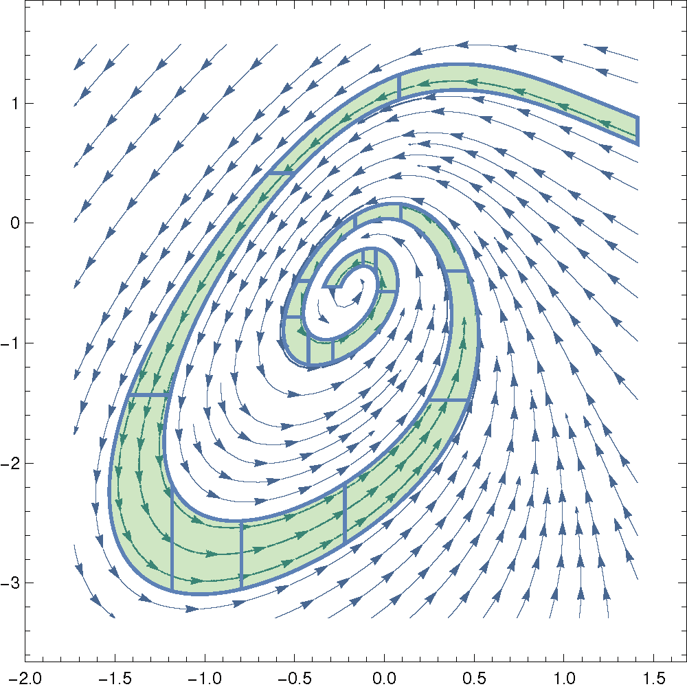
(c) PRBT

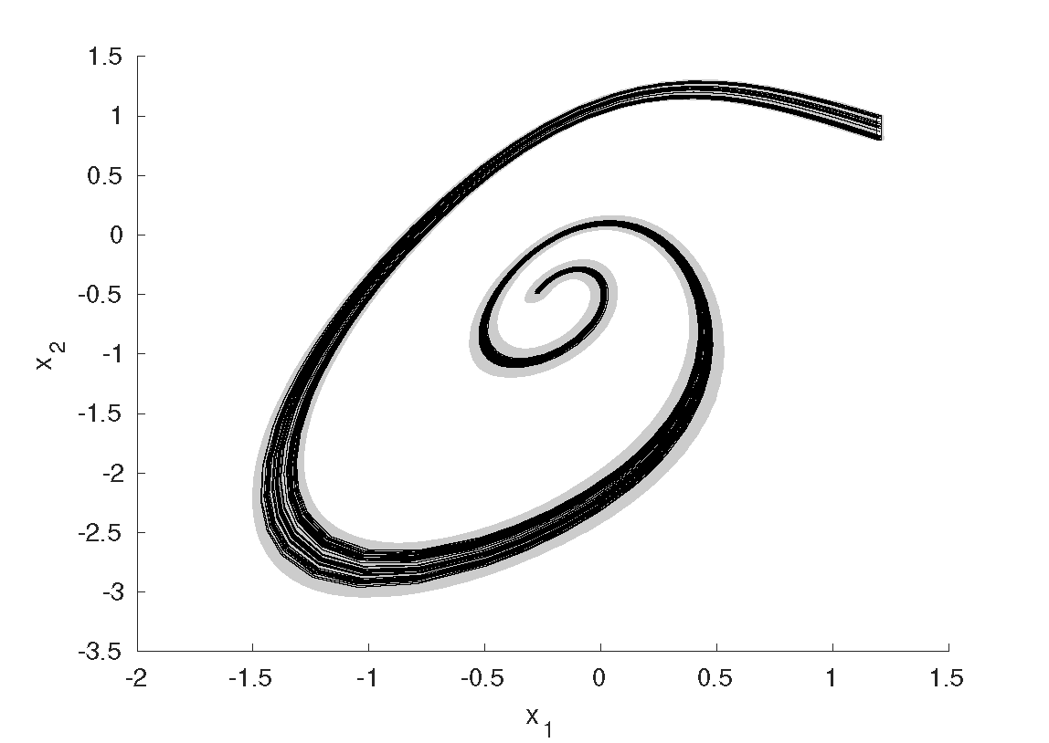
(d) CORA

Figure 4: Buckling Column: (a), (b); Jet Engine: (c), (d)

5.2 Nonlinear Hybrid System

We use the tunnel diode oscillator (TDO) circuit (with different setting) introduced in [20] to illustrate the application of our approach to hybrid system. The two state space variables are the voltage $x_{1}=V_{C}$ across capacitor and the current $x_{2}=I_{L}$ through the inductor. The system dynamics is described as follows,

$$\dot{x}_{1}=\frac{1}{C}(-h(x_{1})+x_{2})\qquad\dot{x}_{2}=\frac{1}{L}(-x_{1}-\frac{x_{2}}{G}+V_{in})$$

where $h(x_{1})$ describes the tunnel diode characteristic and $V_{in}=0.3V$, $G=5m\ {ohm}^{-1}$, $L=0.5\mu H$ and $C=2pF$.

For this model, we want to define an initial state region $\mathit{X_{0}}$ which can guarantee the oscillating behaviour for the system. Due to the highly nonlinear behaviour of the system, a common strategy to deal with this model is to use a hybridized model to approximate the dynamics system and then apply formal verification to the hybrid model[13, 18]. In our experiment, we use three cubic equations to approximate the curve of $h(x_{1})$.

$$h(x_{1})=\left\{\begin{array}[]{lc}0.000847012+35.2297x_{1}-395.261x_{1}^{2}+1372.29x_{1}^{3},\ 0\leq x_{1}\leq 0.0691\\ 1.242-0.033x_{1}-47.4311x_{1}^{2}+116.48x_{1}^{3},\ 0.0691\leq x_{1}\leq 0.3\\ -16.544+139.64x_{1}-389.245x_{1}^{2}+359.948x_{1}^{3},\ 0.3\leq x_{1}\leq 0.50\\ \end{array}\right.$$

From the piecewise function $h(x_{1})$, we can derive a $3$-mode hybrid system which is shown in Figure 5. The system switches between the locations as the value of $x_{1}$ changes.

Figure 5: Hybridized model of TDO

Let the initial set be $\mathit{X_{0}}=\{(x_{1},x_{2})\in\mathbb{R}^{2}\mid 0.40\leq x_{1}\leq 0.48,0.38\leq x_{2}\leq 0.39\}$ on location $l_{3}$, we compute an overapproximation for the flowpipe using PRBT, Flow* and CORA respectively. As illustrated in Figure 6, both PRBT and CORA found an invariant with roughly the same precision, which indicates the model oscillates for the initial set, while Flow* ran into an error.

(a) PRBT

(b) Flow*

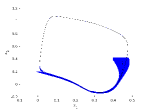
(c) CORA

Figure 6: Flowpipe of hybridized TDO

6 Conclusion

We propose a novel method to compute efficiently a tight overapproximation (flowpipe) of the reachable set for nonlinear continuous and hybrid systems with uncertainty. Our approach avoid the use of interval method for enclosure-box computation, which can produce bigger enclosure-boxes and fewer flowpipe segments. Experiments on several benchmark systems show that our method is more efficient and precise than other popular approaches proposed in literature.

References

- [1] Matthias Althoff and Dmitry Grebenyuk. Implementation of interval arithmetic in CORA 2016. In Proc. of ARCH, volume 43 of EPiC Series in Computing, pages 91–105. EasyChair, 2017.
- [2] Eugene Asarin, Thao Dang, and Antoine Girard. Hybridization methods for the analysis of nonlinear systems. Acta Informatica, 43(7):451–476, 2007.
- [3] Mohamed Amin Ben Sassi, Sriram Sankaranarayanan, Xin Chen, and Erika Ábrahám. Linear relaxations of polynomial positivity for polynomial lyapunov function synthesis. IMA Journal of Mathematical Control and Information, 33(3):723–756, 2015.
- [4] Martin Berz and Kyoko Makino. Verified integration of odes and flows using differential algebraic methods on high-order taylor models. Reliable Computing, 4(4):361–369, 1998.
- [5] Sergiy Bogomolov, Christian Schilling, Ezio Bartocci, Grégory Batt, Hui Kong, and Radu Grosu. Abstraction-based parameter synthesis for multiaffine systems. In Proc. of HVC: the 11th International Haifa Verification Conference on Hardware and Software: Verification and Testing, volume 9434 of LNCS, pages 19–35, 2015.
- [6] Xin Chen, Erika Ábrahám, and Sriram Sankaranarayanan. Flow*: An analyzer for non-linear hybrid systems. In Proc. of CAV 2013: the 25th International Conference on Computer Aided Verification, volume 8044 of LCNS, pages 258–263. Springer, 2013.
- [7] Alessandro Cimatti, Alberto Griggio, Ahmed Irfan, Marco Roveri, and Roberto Sebastiani. Experimenting on solving nonlinear integer arithmetic with incremental linearization. In Proc. of SAT 2018: the 21st International Conference on Theory and Applications of Satisfiability Testing, volume 10929 of LNCS, pages 383–398. Springer, 2018.
- [8] Alessandro Cimatti, Alberto Griggio, Ahmed Irfan, Marco Roveri, and Roberto Sebastiani. Incremental linearization for satisfiability and verification modulo nonlinear arithmetic and transcendental functions. ACM Trans. Comput. Log., 19(3):19:1–19:52, 2018.
- [9] Jacek Cyranka, Md. Ariful Islam, Greg Byrne, Paul L. Jones, Scott A. Smolka, and Radu Grosu. Lagrangian reachabililty. In Proc. of CAV 2017: the 29th International Conference on Computer Aided Verification, volume 10426 of LNCS, pages 379–400. Springer, 2017.
- [10] Jacek Cyranka, Md. Ariful Islam, Scott A. Smolka, Sicun Gao, and Radu Grosu. Tight continuous-time reachtubes for lagrangian reachability. In Proc. of CDC 2018: 57th IEEE Conference on Decision and Control, page to appear. IEEE, 2018.
- [11] Parasara Sridhar Duggirala, Sayan Mitra, Mahesh Viswanathan, and Matthew Potok. C2E2: A verification tool for stateflow models. In Proc. of TACAS 2015: the 21st International Conference on Tools and Algorithms for the Construction and Analysis of Systems, volume 9035 of LNCS, pages 68–82. Springer, 2015.
- [12] Martin Fränzle, Christian Herde, Tino Teige, Stefan Ratschan, and Tobias Schubert. Efficient solving of large non-linear arithmetic constraint systems with complex boolean structure. JSAT, 1(3-4):209–236, 2007.
- [13] G Frehse, BH Krogh, and RA Rutenbar. Verification of hybrid systems using iterative refinement. Proc. SRC TECHCON 2005, Portland, USA, Oct. 24-26, 2005.
- [14] Goran Frehse, Colas Le Guernic, Alexandre Donzé, Scott Cotton, Rajarshi Ray, Olivier Lebeltel, Rodolfo Ripado, Antoine Girard, Thao Dang, and Oded Maler. SpaceEx: Scalable verification of hybrid systems. In Proc. of CAV 2011: the 23rd International Conference on Computer Aided Verification, volume 6806 of LNCS, pages 379–395. Springer, Springer, 2011.
- [15] Antoine Girard and Colas Le Guernic. Efficient reachability analysis for linear systems using support functions. Proc. of IFAC World Congress, 41(2):8966–8971, 2008.
- [16] Radu Grosu, Grégory Batt, Flavio H. Fenton, James Glimm, Colas Le Guernic, Scott A. Smolka, and Ezio Bartocci. From cardiac cells to genetic regulatory networks. In Proc. of CAV 2011: the 23rd International Conference Computer Aided Verification, volume 6806 of LNCS, pages 396–411. Springer, 2011.
- [17] S. Gulwani and A. Tiwari. Constraint-based approach for analysis of hybrid systems. In Proc. of CAV 2008: the 20th International Conference on Computer Aided Verification, volume 5123 of LNCS, pages 190–203. Springer, 2008.
- [18] Smriti Gupta, Bruce H Krogh, and Rob A Rutenbar. Towards formal verification of analog and mixed-signal designs. TECHCON, 2003.
- [19] Amit Gurung, Rajarshi Ray, Ezio Bartocci, Sergiy Bogomolov, and Radu Grosu. Parallel reachability analysis of hybrid systems in xspeed. International Journal on Software Tools for Technology Transfer, to appear:1–23, 2018.
- [20] Walter Hartong, Lars Hedrich, and Erich Barke. Model checking algorithms for analog verification. In Proceedings of the 39th annual Design Automation Conference, pages 542–547. ACM, 2002.
- [21] T.A. Henzinger. The theory of hybrid automata. In Proc. IEEE Symp. Logic in Computer Science, pages 278–292, 1996.
- [22] Hui Kong, Ezio Bartocci, and Thomas A. Henzinger. Reachable set over-approximation for nonlinear systems using piecewise barrier tubes. In Proc. of CAV 2018: the 30th International Conference on Computer Aided Verification, volume 10981 of LNCS, pages 449–467. Springer, 2018.
- [23] Hui Kong, Sergiy Bogomolov, Christian Schilling, Yu Jiang, and Thomas A. Henzinger. Safety verification of nonlinear hybrid systems based on invariant clusters. In Proc. of HSCC 2017: the 20th International Conference on Hybrid Systems: Computation and Control, pages 163–172. ACM, 2017.
- [24] Hui Kong, Fei He, Xiaoyu Song, William NN Hung, and Ming Gu. Exponential-condition-based barrier certificate generation for safety verification of hybrid systems. In Proc. of CAV 2013: the 25th International Conference on Computer Aided Verification, volume 8044 of LNCS, pages 242–257. Springer, 2013.
- [25] Soonho Kong, Sicun Gao, Wei Chen, and Edmund M. Clarke. dReach: -reachability analysis for hybrid systems. In Proc. of TACAS’15: the 21st International Conference on Tools and Algorithms for the Construction and Analysis of Systems, volume 9035 of LNCS, pages 200–205. Springer, 2015.
- [26] Tomas Krilavicius. Hybrid Techniques for Hybrid Systems. PhD thesis, University of Twente, Enschede, Netherlands, 2006.
- [27] Jean B Lasserre. Polynomial programming: Lp-relaxations also converge. SIAM Journal on Optimization, 15(2):383–393, 2005.
- [28] J. Liu, N. Zhan, and H. Zhao. Computing semi-algebraic invariants for polynomial dynamical systems. In Proc. of EMSOFT 2011: the 11th International Conference on Embedded Software, pages 97–106. ACM, 2011.
- [29] Nadir Matringe, Arnaldo Vieira Moura, and Rachid Rebiha. Generating invariants for non-linear hybrid systems by linear algebraic methods. In Proc. of SAS 2010: the 17th International Symposium on Static Analysis, volume 6337 of LNCS, pages 373–389. Springer, 2010.
- [30] Nedialko S Nedialkov. Interval tools for ODEs and DAEs. In Proc. of SCAN 2006: the 12th GAMM - IMACS International Symposium on Scientific Computing, Computer Arithmetic and Validated Numerics, pages 4–4. IEEE, 2006.
- [31] Pavithra Prabhakar and Miriam García Soto. Hybridization for stability analysis of switched linear systems. In Proc. of HSCC 2016: of the 19th Intern. Conference on Hybrid Systems: Computation and Control, pages 71–80. ACM, 2016.
- [32] S. Prajna and A. Jadbabaie. Safety verification of hybrid systems using barrier certificates. Proc. of HSCC 2004: the 7th International Workshop on Hybrid Systems: Computation and Control, 2993:271–274, 2004.
- [33] Mihai Putinar. Positive polynomials on compact semi-algebraic sets. Indiana University Mathematics Journal, 42(3):969–984, 1993.
- [34] Rajarshi Ray, Amit Gurung, Binayak Das, Ezio Bartocci, Sergiy Bogomolov, and Radu Grosu. Xspeed: Accelerating reachability analysis on multi-core processors. In Proc. of HVC 2015: the 11th International Haifa Verification Conference on Hardware and Software: Verification and Testing, volume 9434 of LNCS, pages 3–18. Springer, 2015.
- [35] Nima Roohi, Pavithra Prabhakar, and Mahesh Viswanathan. Hybridization based CEGAR for hybrid automata with affine dynamics. In Proc. of TACAS 2016: the 22nd International Conference on Tools and Algorithms for the Construction and Analysis of Systems, volume 9636 of LNCS, pages 752–769. Springer, 2016.
- [36] S. Sankaranarayanan. Automatic invariant generation for hybrid systems using ideal fixed points. In Proc. of HSCC 2010: the 13th ACM International Conference on Hybrid Systems: Computation and Control, pages 221–230. ACM, 2010.
- [37] S. Sankaranarayanan, H. Sipma, and Z. Manna. Constructing invariants for hybrid systems. In Proc. of HSCC 2004: the 7th Intern. Workshop on Hybrid Systems: Computation and Control, volume 2993 of LNCS, pages 539–554. Springer, 2004.
- [38] Sriram Sankaranarayanan, Xin Chen, et al. Lyapunov function synthesis using handelman representations. IFAC Proceedings Volumes, 46(23):576–581, 2013.
- [39] Stefan Schupp, Erika Ábrahám, Ibtissem Ben Makhlouf, and Stefan Kowalewski. Hypro: A C++ library of state set representations for hybrid systems reachability analysis. In Proc. of NFM 2017: the 9th International Symposium on NASA Formal Methods, volume 10227 of LNCS, pages 288–294, 2017.
- [40] Andrew Sogokon, Khalil Ghorbal, Paul B Jackson, and André Platzer. A method for invariant generation for polynomial continuous systems. In Proc. of VMCAI 2016: the 17th International Conference on Verification, Model Checking, and Abstract Interpretation, volume 9583 of LNCS, pages 268–288. Springer, 2016.
- [41] Gilbert Stengle. A Nullstellensatz and a Positivstellensatz in semialgebraic geometry. Mathematische Annalen, 207(2):87–97, 1974.
- [42] A. Taly and A. Tiwari. Deductive verification of continuous dynamical systems. In FSTTCS, volume 4, pages 383–394, 2009.
- [43] Zhengfeng Yang, Chao Huang, Xin Chen, Wang Lin, and Zhiming Liu. A linear programming relaxation based approach for generating barrier certificates of hybrid systems. In International Symposium on Formal Methods, pages 721–738. Springer, 2016.