Dynamical band gap tuning in Weyl semi-metals by intense elliptically polarized normal illumination and its application to $8-Pmmn$ borophene.

Abstract

The Dynamical-gap formation in Weyl semimetals modulated by intense elliptically polarized light is addressed through the solution of the time-dependent Schrödinger equation for the Weyl Hamiltonian via the Floquet theorem. The time-dependent wave functions and the quasi-energy spectrum of the two-dimensional Weyl Hamiltonian under normal incidence of elliptically polarized electromagnetic waves are obtained using a non-perturbative approach. In it, the Weyl equation is reduced to an ordinary second-order differential Mathieu equation. It is shown that the stability conditions of the Mathieu functions are directly inherited by the wave function resulting in a quasiparticle spectrum consisting of bands and gaps determined by dynamical diffraction and resonance conditions between the electron and the electromagnetic wave. Estimations of the electromagnetic field intensity and frequency, as well as the magnitude of the generated gap are obtained for the $8-Pmmn$ phase of borophene. We provide with a simple method that enables to predict the formation of dynamical-gaps of unstable wave functions and their magnitudes. This method can readily be adapted to other Weyl semimetals.

Keywords

Weyl semi-metals; dynamical gap; Mathieu equation

I Introduction

Recently, the so-called Dirac and Weyl materials have received considerable attention due to their possible implementation into next-generation electronic devices Novoselov et al. (2012); Peng et al. (2016); Ferrari et al. (2015); Naumis et al. (2017). The main physical properties of these materials were observed for the first time in graphene, an allotrope of carbon consisting of a monolayer of atoms in a honeycomb lattice with an electron linear dispersion near the Dirac points. As a result of this characteristics, the charge carriers in graphene behave like massless Dirac fermions Geim (2009); Neto et al. (2009); Oliva-Leyva and Naumis (2014); Naumis and Roman-Taboada (2014); Oliva-Leyva and Naumis (2015a, b, c); Naumis et al. (2017); Carrillo-Bastos and Naumis (2018). Thereafter, a wide variety of two-dimensional materials with similar properties has been discovered Wehling et al. (2014). Examples of these are: silicene Jose and Datta (2013); Liu et al. (2013), germanene Behera and Mukhopadhyay (2011); Zhang et al. (2016a), stanene Zhu et al. (2015); Chen et al. (2016) and artificial graphene Soltan-Panahi et al. (2011); Gomes et al. (2012). Borophen, a two dimensional allotrope of boron, also falls in this category. The chemical similarity between boron and carbon atoms has triggered the search for stable two-dimensional boron structures and synthesis techniques to produce themZhang et al. (2017). Since their theoretical prediction Boustani (1997), many different allotropes of borophene have been experimentally confirmed Mannix et al. (2015). Among its many different phases, the orthorhombic $8-Pmmn$ is one of the most energetically stable structures Peng et al. (2016), having a ground state energy lower than its analogs Verma et al. (2017). Borophene, in contrast with graphene, shows a highly anisotropic crystalline structure, which causes high optical anisotropy and transparency Peng et al. (2016); Verma et al. (2017); Champo and Naumis (2019). It is thus a strong candidate for flexible electronics, display technologies and in the design of smart windows where minimal photon absorption and reflection are required Zhang et al. (2016b); Peng et al. (2016); Zhang et al. (2017).

Despite the many useful and fascinating properties of graphene, borophene and Weyl materials in general, their lack of an electronic band gap has stimulated the search for either other two-dimensional materials with semiconducting properties or techniques to induce them artificially. Among other proposals to circumvent this problem, one of the most promising ideas is generating a light induced dynamical-gap. As the electromagnetic field is a periodical function of time, this technique has been termed Floquet gap engineering. High intensity electromagnetic waves interacting with graphene have been studied using perturbative approaches López-Rodríguez and Naumis (2010); Higuchi et al. (2017). However, it has been shown that light induces a renormalization of the electronic spectrum of Dirac materials not captured by simple perturbation techniques López-Rodríguez and Naumis (2008, 2010); Kibis (2010); Kristinsson et al. (2016a); Oliva-Leyva and Naumis (2016); Kristinsson et al. (2016b); Kibis et al. (2017). In this regard, borophene brigns interesting possibilities to study the light-matter interaction in Weyl semimetals due to its asymmetric spectrum. As graphene, borophene has a honeycomb lattice with two nonequivalent sublattices. However, its peculiar structure give rise to a tilted anisotropic cone in the vicinity of the Dirac points Islam and Jayannavar (2017); Verma et al. (2017); Champo and Naumis (2019), as opposed to graphene whose spectrum is completely isotropic in $K$ space.

Recently, the formation of energy gaps in borophene subject high-intensity linearly polarized light was studied beyond the perturbative approximation Champo and Naumis (2019). It was found that borophene, when interacting with light, acquires a complex band structure from the stability conditions of the solutions of the Mathieu differential equation. Among other effects, the interaction with light produces a gap in the vicinity of borophene’s Dirac point. The effects of an intense circularly polarized electromagnetic field have, nevertheless, not been discussed for borophene yet.

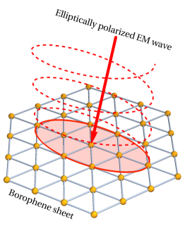
Figure 1: Borophene sheet under an elliptically polarized electromagnetic wave.

In this paper, we address the general problem of a particle that obeys the Weyl Hamiltonian subject to an intense elliptically polarized electromagnetic field. As it is schematized in Fig. 1, our solutions can be applied to the particular case of electrons in borophene under a strong elliptically polarized field. We report the wave functions, the quasi-energy spectrum, and the magnitude of the dynamic gap opening. The case of linearly polarized light, addressed by us previously Champo and Naumis (2019), is proven to be fundamentally different from the elliptically polarized one studied in this work. Our analysis mainly focuses on the stability and instability of the time-dependent wave functions. The results presented here display an interesting interplay between the tilted anisotropy and the relative orientation of the light-polarization ellipse. Moreover, we show that the gaps may be tuned by changing the orientation of the elliptical polarization profile of light.

The paper is organized as follows. In Sec. II we introduce the low-energy effective two-dimensional Weyl Hamiltonian under an arbitrary electromagnetic field. Subsequently, in Sec. III, we determine the time-dependent wavefunction of electrons in borophene subject to an elliptically polarized electromagnetic field. In this same section we analyze the stability of the solutions inherited from Mathieu functions in the strong electromagnetic field or long wavelength regimes. We workout the time-dependent wave functions and the solutions’ stability chart. To get an insight into the gap structure, in Sec. III.2, the stability and instability regions are projected onto the tilted Dirac cones of the free Weyl electrons. In Sec. III.2, we extract the quasi-energy spectrum from the time-dependent wave function and prove that it consistently shows a similar gap structure to that of the projected chart. Finally, we summarize and conclude in Sec. IV.

II Weyl electrons subject to electromagnetic fields

II.1 The Weyl Hamiltonian

The single-particle low-energy effective Weyl Hamiltonian is given by Zabolotskiy and Lozovik (2016); Islam and Jayannavar (2017); Verma et al. (2017); Champo and Naumis (2019),

$$\hat{H}=\mu\left(v_{t}\hat{P}_{y}\hat{\sigma}_{0}+v_{x}\hat{P}_{x}\hat{\sigma}_{x}+v_{y}\hat{P}_{y}\hat{\sigma}_{y}\right),$$ (1)

where $\hat{P}_{x}$ and $\hat{P}_{y}$ are the momentum operators, $\hat{\sigma}_{i}$ are the Pauli matrices, and $\hat{\sigma}_{0}$ is the $2\times 2$ identity matrix. For $8-Pmmn$ borophene, the three velocities in the Weyl Hamiltonian (1) are $v_{x}=0.86v_{F}$, $v_{y}=0.69v_{F}$ and $v_{t}=0.32v_{F}$ in units of the Fermi velocity $v_{F}=10^{6}\,m/s$ Zabolotskiy and Lozovik (2016). The two Dirac points $\mathbf{k}=\pm\mathbf{k}_{D}$ are given by the valley index $\mu=\pm 1$. The first term in Eq. (1) gives rise to the tilting of the Dirac cones and the last ones correspond to the kinetic energy.

The previous Hamiltonian results in the energy dispersion relation Islam and Jayannavar (2017)

$$E_{\eta,k}^{\mu}=\mu\hbar v_{t}k_{y}+\eta\epsilon,$$ (2)

where

$$\epsilon=\hbar\sqrt{v_{x}^{2}k_{x}^{2}+v_{y}^{2}k_{y}^{2}}.$$ (3)

The corresponding free Weyl electron wave function is,

$$\psi_{\eta,\,\bf{k}}^{\mu}(\mathbf{r})=\mu\frac{\exp(i\bf{k\cdot r})}{\sqrt{2}}\left[\begin{array}[]{lcc}1\\ \eta\exp(i\Theta)\end{array}\right],$$ (4)

where $\eta=\pm 1$ is the band index, $\Theta=\tan^{-1}(v_{y}k_{y}/v_{x}k_{x})$ and the two-dimensional momentum vector is given by $\mathbf{k}=(k_{x},k_{y})$.

II.2 The Weyl Hamiltonian in the presence of an electromagnetic wave

Now we consider a charge carrier described by the Weyl Hamiltonian subject to an electromagnetic wave that propagates along a direction perpendicular to the surface of the crystal. From Eq. (1) and using the minimal coupling we obtain,

$$\hat{H}=\left(\begin{array}[]{lcc}v_{t}\hat{\Pi}_{y}&v_{x}\hat{\Pi}_{x}-iv_{y}\hat{\Pi}_{y}\\ v_{x}\hat{\Pi}_{x}+iv_{y}\hat{\Pi}_{y}&v_{t}\hat{\Pi}_{y}\end{array}\right),$$ (5)

where $\hat{\boldsymbol{\Pi}}=\hat{\boldsymbol{P}}-e{\boldsymbol{A}}$, with $\boldsymbol{A}=(A_{x},A_{y})$ being the vector potential of the incident electromagnetic wave. Calculations are considerably simplified by choosing a gauge in which the vector potential is only a function of time. The Schrödinger equation for charge carriers in a Weyl semimetal is thus given by

$$\hat{H}(\mathbf{r},t){\boldsymbol{\Psi}}(\boldsymbol{r},t)=i\hbar\frac{\partial}{\partial t}{\boldsymbol{\Psi}}(\boldsymbol{r},t),$$ (6)

where, in the two dimensional spinor $\boldsymbol{\Psi}(\mathbf{r},t)=\left(\Psi_{A}(\mathbf{r},t),\Psi_{B}(\mathbf{r},t)\right)^{\top}$, $A$ and $B$ label the two sublattices.

To deduce the explicit form of the wave function ${\bf{\Psi}}(\mathbf{r},t)$ from Eq. (6) we make the following ansatz

$$\mathbf{\Psi}(\mathbf{r},t)=\exp{\left(i\mathbf{k}\cdot\mathbf{r}\right)}\mathbf{\Phi}(t),$$ (7)

where $\mathbf{\Phi}(t)=\left(\Phi_{A}(t),\Phi_{B}(t)\right)^{\top}$. Substituting (7) reduces Eq. (6) into

$$\mathbbm{H}(t)\mathbf{\Phi}(t)=i\hbar\frac{d}{dt}\mathbf{\Phi}(t),$$ (8)

where the matrix $\mathbbm{H}(t)$ is defined in Appendix A.

The diagonal terms of $\mathbbm{H}(t)$ can be lifted by explicitly adding a time-dependent phase to the wave function

$$\mathbf{\Phi}(t)=\exp{\left[-\frac{i}{\hbar}\int^{t}ds\alpha_{\mathbf{k}}(s)\right]}{\bm{\chi}}(t),$$ (9)

with $\alpha_{\mathbf{k}}(t)=\hbar v_{t}k_{y}-ev_{t}A_{y}(t)$ and $\bm{\chi}(t)=(\chi_{A}(t),\chi_{B}(t))^{\top}$. Following the procedure shown in the Appendix A, Eq. (8) can be recast in the form of a second-order ordinary differential equation as

$$\frac{d^{2}}{dt^{2}}\bm{\chi}(t)+\mathbbm{F}(t)\bm{\chi}(t)=0,$$ (10)

where the function $\mathbbm{F}(t)$ is defined by

$$\mathbbm{F}(t)=-\frac{i}{\hbar}\hat{\bm{\sigma}}\cdot\frac{d\bm{S}}{dt}+\frac{1}{\hbar^{2}}\left[\widetilde{\mathbbm{H}}(t)\right]^{2},$$ (11)

with $[\widetilde{\mathbbm{H}}(t)]^{2}=|\boldsymbol{\kappa}_{\boldsymbol{v}}-\boldsymbol{S}|^{2}$, $\boldsymbol{\kappa}_{\boldsymbol{v}}=\hbar(v_{x}k_{x},v_{y}k_{y})$ and $\boldsymbol{S}=e(v_{x}A_{x},v_{y}A_{y})$. In the last expression, the vector $\boldsymbol{\kappa}_{\boldsymbol{v}}$ is the directional energy flux of the electrons, and the components of $\boldsymbol{S}$ represent the work done by the electromagnetic wave along the $x$ and $y$ directions.

III Elliptically polarized waves

Let us now study the case of an elliptically polarized electromagnetic wave characterized by the vector potential

$${\bf{A}}=\frac{1}{\Omega}\left(E_{x}\cos(\Omega t),E_{y}\sin(\Omega t)\right),$$ (12)

where $E_{x}$ and $E_{y}$ are constants and $\Omega$ is the frequency of the electromagnetic wave. The vector potential (12) corresponds to the electric field $\bm{E}=-\partial\boldsymbol{A}/\partial t=(E_{x}\sin(\Omega t),-E_{y}\cos(\Omega t))$.

Rewriting Eq. (10) in terms of the phase

$$\phi=\Omega t,$$ (13)

yields the Hill equation Magnus and Winkler (2013)

$$\bm{\chi}^{\prime\prime}(\phi)+\mathbbm{F}(\phi)\bm{\chi}(\phi)=0,$$ (14)

where $\mathbbm{F}(\phi)$ is

$$\mathbbm{F}(\phi)=i\left(\frac{\zeta_{x}}{\hbar\Omega}\hat{\sigma}_{x}\sin\phi-\frac{\zeta_{y}}{\hbar\Omega}\hat{\sigma}_{y}\cos\phi\right)\\ +\left(\frac{1}{\hbar\Omega}\right)^{2}\left[\epsilon^{2}-2\bm{\kappa}_{\bm{v}}\cdot\bm{S}+\frac{1}{2}\left(\zeta^{2}_{x}+\zeta^{2}_{y}\right)\right.\\ \left.+\frac{1}{2}\left(\zeta^{2}_{x}-\zeta^{2}_{y}\right)\cos(2\phi)\right],$$ (15)

and

$$\bm{S} = (\zeta_{x}\cos\phi,\zeta_{x}\sin\phi),$$ (16)

$$\zeta_{x} = eE_{x}v_{x}/\Omega,$$ (17)

$$\zeta_{y} = eE_{y}v_{y}/\Omega.$$ (18)

The unitless parameter $\epsilon/\hbar\Omega$ is the ratio of the electron energy to the photon energy. Similarly, the parameter $\zeta_{x}/\hbar\Omega$ ($\zeta_{y}/\hbar\Omega$) is the ratio of the work done by the electromagnetic wave along the $x$ ($y$) direction to the photon energy.

The determination of the stability regions of the differential Eq. (14) is quite challenging mainly due to the imaginary part in the first term of the right-hand side of Eq. (15). While the real part gives rise to the Whittaker-Hill equationUrwin and Arscott (1970), the imaginary term yields a Mathieu-like equation with complex characteristic values, rarely discussed in literature Ziener et al. (2012). Fortunately, in the intense electric field or long wavelength regimes the imaginary part is negligible. Other limits are treatable by perturbation theory López-Rodríguez and Naumis (2010); Higuchi et al. (2017).

Here we focus on the intense electric field regime. We thus assume that $\zeta_{i}/\hbar\Omega\gg 1$ with $i=x,\,y$, which is equivalent to $ecE_{x}/\hbar\Omega^{2}\gg 349$ and $ecE_{y}/\hbar\Omega^{2}\gg 435$. This corresponds to electric fields $E_{x}\gg 1.91\,V/m$ and $E_{y}\gg 2.39\,V/m$. Thereby, we can neglect the linear terms of $\zeta_{i}/\hbar\Omega$ in Eq. (14) that yield the imaginary terms. The obtained expression, best-known for describing the dynamics of the parametric pendulumAldrovandi and Ferreira (1980); Baker and Blackburn (2005), is the Mathieu differential equation

$$\bm{\chi}^{\prime\prime}(\phi)+[a-2q\cos(2\phi)]\bm{\chi}(\phi)=0.$$ (19)

The purely real parameters $q$ and $a$ are given by

$$q = \frac{\zeta^{2}_{y}-\zeta^{2}_{x}}{\left(2\hbar\Omega\right)^{2}}=\left(\frac{e}{2\hbar\Omega^{2}}\right)^{2}\left(v^{2}_{y}E^{2}_{y}-v^{2}_{x}E^{2}_{x}\right),$$ (20)

$$a = \frac{\epsilon^{2}+\zeta^{2}_{y}}{\left(\hbar\Omega\right)^{2}}-2q=\frac{2\epsilon^{2}+\zeta^{2}_{x}+\zeta^{2}_{y}}{2\left(\hbar\Omega\right)^{2}}$$ (21)

$$\,\,\,\,\,=\frac{\epsilon^{2}}{\left(\hbar\Omega\right)^{2}}+\left(\frac{e}{\hbar\Omega^{2}}\right)^{2}\left(v^{2}_{x}E^{2}_{x}+v^{2}_{y}E^{2}_{y}\right).$$

The characteristic value of the Mehtieu equation

$$\sqrt{a}=\frac{\Omega_{0}}{\Omega},$$ (22)

with $\Omega_{0}=\sqrt{2\epsilon^{2}+\zeta^{2}_{x}+\zeta^{2}_{y}}/\sqrt{2}\hbar$ is the ratio between the fundamental frequency $\Omega_{0}$ and the frequency of the electromagnetic wave $\Omega$. The characteristic value $a$ parametrizes the family of ellipses in the $k_{x}-k_{y}$ plane that are characterized by the eccentricity $[1-(v_{y}^{2}/v_{x}^{2})]^{1/2}$. Stated differently, each value of the parameter $a$ corresponds to a particular elliptical section of the Dirac cone. However, not all the ordered pairs in the $q-a$ plane produce stable solutions of the Mathieu equation. Consequently, in the presence of an intense electromagnetic radiation not all the elliptical sections of the Dirac cones correspond to stable solutions. In fact, the interaction with light induces elliptical sections of the Dirac cone that alternate between forbidden (unstable) and allowed (stable) solutions. As can be seen in Fig. 2, the stability chart in the $q-a$ plane consists of tongue-like stable regions (light blue) that neighbor with unstable regions (white). The Mathieu equation might have either even or odd stable solutions. Even stable solutions of (19) have the form

$$\boldsymbol{\chi}(\phi)=\mathcal{C}(a,q,\phi)=\exp[-ir(a,q)\phi]\boldsymbol{f}_{C}(\phi),$$ (23)

where $\mathcal{C}(a,q,\phi)$ is the even Mathieu function, $\boldsymbol{f}_{C}(\phi)$ is an even function with period $\pi$ and $a=a_{r}(q)$ is the Mathieu even characteristic value. Conversely, odd stable solutions have the form

$$\boldsymbol{\chi}(\phi)=\mathcal{S}(a,q,\phi)=\exp[-ir(b,q)\phi]\boldsymbol{f}_{S}(\phi),$$ (24)

where $\mathcal{S}(a,q,\phi)$ is the odd Mathieu function, $\boldsymbol{f}_{S}(\phi)$ is an odd function with period $\pi$ and $b=b_{r}(q)$ is the Mathieu odd characteristic value. When $r$ is a non-integer rational number, inside the stable regions, the even and odd characteristic values are identical, namely $a_{r}(q)=b_{r}(q)$. The rational function $r(a,q)$ depends on the Mathieu characteristic value $a$ and the parameter $q$. On the boundaries between the stable and unstable regions (solid and dashed blue lines Fig. 2) $r$ takes an integer value and inside the stable regions $r$ is a non-integer rational number. Thus, inside the stability regions the even and odd Mathieu functions have the same characteristic value. For the particular situation in which $q=0$, (19) reduces to the differential equation of an harmonic oscillator whose solutions are $\cos(\sqrt{a}\phi)$ and $\sin(\sqrt{a}\phi)$ McLachlan (1951). Evidently, in this case $r=\sqrt{a}$. Moreover, in the special case where $r=\sqrt{a}\in\mathbbm{Z}$, resonant states are generated for which

$$\frac{\Omega_{0}}{\Omega}=1,\,2,\,3,...,$$ (25)

and therefore when $q\to 0$ two contiguous stability zones are connected.

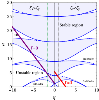
Figure 2: Mathieu equation stability chart of in the $q-a$ plane. The stability (light blue) and instability (white) domains are divided by the characteristic curves $a_{r}(q)$ (solid blue lines) and $b_{r}(q)$ (dashed blue lines) where $r\in\mathbbm{Z}$. The Mathieu characteristic values $a_{r}(q)$ and $b_{r}(q)$ have even parity with respect to $q$ and therefore the spectrum is symmetric for $\zeta_{x}>\zeta_{y}$ and $\zeta_{x}<\zeta_{y}$. The solid purple ($\zeta_{x}>\zeta_{y}$) and red ($\zeta_{x}<\zeta_{y}$) lines correspond to the extra constraint due to Eq. (21). The vertical dotted green line corresponds to $q=-1.77$ and the dotted gray line to $q=0.87$.

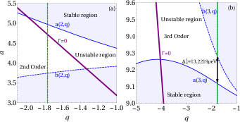
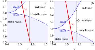
Figure 3: Zoom of the stability chart near $\Gamma=0$ ($\epsilon=0$ and $E^{+}_{\pm 1,k}-\hbar v_{t}k_{y}=0$) in the long wavelength regime. (a) Crossing of the vertical line $q=-1.77$ (green dotted line) and condition (27) (purple solid line). The crossing falls inside an unstable state region. (b) Third-order energy gap $\Delta^{L}_{3}$ in the $q<0$ region ($\zeta_{x}>\zeta_{y}$) for fixed fields $E_{x}=5.5$ V/m and $E_{y}=2.6$ V/m. (c) Crossing of the vertical line $q=0.87$ (gray dotted line) and condition (27) (red solid line). The crossing falls inside a stable state region. (d) Second-order energy gap $\Delta^{R}_{2}$ in the $q>0$ region ($\zeta_{x}<\zeta_{y}$) for fixed fields $E_{x}=2.6$ V/m and $E_{y}=5.5$ V/m. In all the panels the microwave frequency is $\Omega=50$ GHz.

III.1 Wave function and stability spectrum

The general solution of Eq. (19) is the superposition of the even and odd Mathieu functions $\mathcal{C}(a,q,\phi)$ and $\mathcal{S}(a,q,\phi)$. The wave function is then given by

$$\boldsymbol{\Psi}(\bm{r},t)=\mathcal{N}\exp\left[i\left(\boldsymbol{k}\cdot\boldsymbol{r}-v_{t}k_{y}t-\frac{v_{t}\zeta_{y}}{v_{y}\hbar\Omega}\cos(\Omega t)\right)\right]\\ \times\left[\,\mathcal{C}(a,q,\Omega t)\pm i\eta\mathcal{S}(a,q,\Omega t)\,\right]\left(\begin{array}[]{lcc}1\\ \eta\exp(i\Theta)\end{array}\right),$$ (26)

where $\mathcal{N}$ is a normalization constant, $\Theta=\tan^{-1}\left(v_{y}k_{y}/v_{x}k_{x}\right)$, and $\eta=\pm 1$ denotes the conduction and valence bands, respectively. The wave function (26) reduces to the free-particle wave function (4) when the electric field vanishes.

Since the time-dependent wave function is expressed in terms of the Mathieu functions, its stability is governed by the stability chart in 2 that we discussed previously. Indeed, the structure of the dynamical gaps of Weyl electrons, generated in the presence of an intense electromagnetic radiation, is inherited from the properties of the characteristic values of the Mathieu functions.

The chart can be divided into two key regions according to the shape of the electromagnetic wave: $q<0$ ($\zeta_{x}>\zeta_{y}$) and $q>0$ ($\zeta_{y}>\zeta_{x}$) and $q=0$ ($\zeta_{x}=\zeta_{x}$). If $\zeta_{x}>\zeta_{y}$ ($E_{x}v_{x}>E_{y}v_{y}$) the work done by the electromagnetic wave on the electrons is higher along the $x$ axis. Conversely, if $\zeta_{x}<\zeta_{y}$ ($E_{x}v_{x}<E_{y}v_{y}$) the work is higher along $y$. Finally, if $\zeta_{x}=\zeta_{y}$ ($E_{x}v_{x}=E_{y}v_{y}$) the electromagnetic wave contributes with equal amounts of work in each direction. Nevertheless, the electron state can not access any point $(q,a)$ in the stability chart shown in Fig. 2; Eq. (21) imposes an extra constraint. Defining $\Gamma=\epsilon/\hbar\Omega=\sqrt{v_{x}^{2}k_{x}^{2}+v_{y}^{2}k_{y}^{2}}/\Omega$, Eq. (21) takes the form of a straight line $a=\Gamma^{2}+(\zeta_{y}/\hbar\Omega)^{2}-2q$ in the $q-a$ plane. Hence, for any state to be accessible to the electron, the ordered pair $(q,a)$ must satisfy the inequality

$$a\geq\left(\frac{\zeta_{y}}{\hbar\Omega}\right)^{2}-2q.$$ (27)

In Fig. 2 the solid purple and solid red lines illustrate the limiting case

$$a=(\zeta_{y}/\hbar\Omega)^{2}-2q,$$ (28)

for $\zeta_{x}>\zeta_{y}$ and $\zeta_{y}>\zeta_{x}$ respectively. Naturally, any of these points should also fall on the stable regions allowed by the Mathieu equation in order to produce a stable solution of the wave function.

For fixed $E_{x}$, $E_{y}$ and $\Omega$, $q$ is constant, and therefore the allowed states should be located on the vertical line $q=\mathrm{const}$ (see for example the green dotted line or the gray dotted line in Figs. 2 and 3). Along this lines, the ranges of stable and unstable states alternate producing the appearance of bands separated by dynamical energy gaps. The opening of these gaps is due to the space-time diffraction of electrons in phase with the electromagnetic field, and effect akin to the magnetoacoustic diffraction of electrons in phase with acoustic waves Landau (1946); Davydov (1980); Champo and Naumis (2019).

To further comprehend the connection between the Mathieu stability chart and the consequent wave function gap structure, it is illustrating to project the stable and unstable regions of Fig. 2 on the surface of the tilted Dirac cones that arise from the free particle Weyl equation. To this end, we explicitly express the normalized energy dispersion $\widetilde{E}=(1/\hbar\Omega)E^{+}_{\pm 1,k}$ from Eq. (2) in terms of the normalized wave vector components $(\widetilde{k}_{x},\widetilde{k}_{y})$ and the parameter $a$ in the Eq. (21) obtaining

$$\left(\frac{v_{x}}{v_{F}}\right)^{2}\widetilde{k}^{2}_{x}+\left(\frac{v_{y}}{v_{F}}\right)^{2}\widetilde{k}^{2}_{y}=a+2q-\left(\frac{\zeta_{y}}{\hbar\Omega}\right)^{2},$$ (29)

where $\widetilde{k}_{x}=(v_{F}/\hbar\Omega)k_{x}$ and $\widetilde{k}_{y}=(v_{F}/\hbar\Omega)k_{y}$. Elliptical rings of allowed and forbidden states form in the $(\widetilde{k}_{x},\widetilde{k}_{y})$ plane or on the surface of the Dirac cone for fixed values of $E_{x}$ and $E_{y}$ (or fixed values of $q$ and $\zeta_{y}/\hbar\Omega$). The dressed Dirac cones, the Dirac cones over whose surfaces the allowed and forbidden states have been projected, are shown in Fig. 4. The light blue portion of the surface represents the allowed states and the white rings are the forbidden ones. The first correspond to the stable regions and the latter to the unstable regions of Fig. 2.

In Figs. 3 (a) and (b) we plot the vertical line $q=-1.77$ (green dotted line) and the line (28) (solid purple line) superimposed to a zoom of the stability chart for typical electromagnetic field values $E_{x}=5.5$ V/m, $E_{y}=2.6$ V/m and $\Omega=50$ GHz. The crossing between these two lines, seen in Fig. 3 (a), is the starting point for the search of stable solutions. However, in the immediate region above the crossing we observe a gap of unstable solutions, that projected on to the Dirac cone produces the appearance of forbidden states at the tip, forming a gap. At higher energies, we observe the rings corresponding to the third order gap as can be appreciated in Figs. 2 and 3 (b). This gap yields and energy range $\Delta^{L}_{3}=13.22\,\mu$eV (see Appendix B) of forbidden states. It should be noted that the origins of the first gap at the Dirac point and the following ring-like forbidden regions are essentially the same. Both of them are generated in points that comply with the inequality (27), and as a result of inherent instabilities of the Mathieu solutions.

When the parameters are chosen to fall on the opposite side of the stability chart ($\zeta_{x}<\zeta_{y}$) the arrangement of the gaps is quite different. In Fig. 3 (c) we observe the crossing of the vertical line $q=0.87$ and the limiting line (28) for electromagnetic field values $E_{x}=2.6$ V/m, $E_{y}=5.5$ V/m and $\Omega=50$ GHz. In contrast to the previous case, above the crossing we find ourselves well inside a stability region. Hence, the tip of the Dirac cone is dressed entirely with allowed states and the forbidden rings appear well above it as can be seen in Fig. 4. At high energies the line $q=0.87$ crosses the second order gap as can be seen in Fig. 3 (d). A ring of unstable states with an energy gap of $\Delta^{R}_{2}=19.45\,\mu$eV is projected on to the Dirac cone until the line reaches the next stability zone [see Fig. 4 (b)].

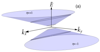
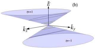
Figure 4: Dirac cones-energy dispersion $\widetilde{E}$ ($\widetilde{k}_{x},\,\widetilde{k}_{y}$) ($E^{+}_{\pm 1}/\hbar\Omega$), for the conduction $\eta=+1$ and valence $\eta=-1$ bands. (a) A gap opens up a the tip of the Dirac cone for $\zeta_{x}>\zeta_{y}$ ($E_{x}=5.5$ V/m and $E_{y}=2.6$ V/m). (b) When $\zeta_{x}<\zeta_{y}$ ($E_{x}=2.6$ V/m and $E_{y}=5.5$ V/m) gaps only open up far from Dirac point. The white regions correspond to forbidden energies and the blue ones to the allowed energies.

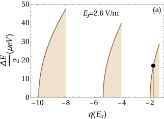
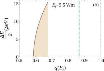
Figure 5: Energy gap ($\Delta E(q)/2$) regions near the Dirac points. The brown solid lines represent $\Delta E/2$ as a function of $q$ in the domains where $\Delta E(q)>0$ for (a) $E_{y}=2.6$ V/m and $\zeta_{x}>\zeta_{y}$, and (b) $E_{y}=5.5$ V/m and $\zeta_{x}<\zeta_{y}$. The vertical dotted gray line and the dot in $q=-1.77$ (a) correspond to $E_{x}=5.5$ V/m, $\Delta E/2=17\,\mu$eV. Likewise, the vertical dotted green line corresponds to $q=0.87$ (b).

To systematize the search of gaps in the $K$ point of the Dirac cone we define the indicator

$$\Delta E(q)/2=\hbar\Omega\sqrt{c_{r}(q)-\left[\left(\frac{\zeta_{y}}{\hbar\Omega}\right)^{2}-2q\right]},$$ (30)

where $r\in\mathbbm{Z}$ and $c_{r}(q)$ is either $a_{r}(q)$ or $b_{r}(q)$, depending on which one is at the bottom of the allowed band. This indicator corresponds to the energy difference between the lower allowed band edge and the limiting case of the inequality (27) given by (28). The integer $r$ is chosen so that the purple line in Fig. 2 is situated directly below the top band edge associated with the stable region. Therefore, if for a given value of $q$ the purple line falls on a forbidden region of states then $\Delta E(q)>0$. If, on the other hand, the purple line falls on an allowed band $\Delta E(q)$ is a pure imaginary number. The domain where $\Delta E(q)$ is a pure real number corresponds, thus, to a gap of forbidden states. Hence, the function $E(q)$ provides with a clear-cut criterion to detect the formation of gaps in the surroundings of the Dirac point: $\Delta E(q)\in\mathbbm{R}$.

In Fig. 5 we analyze the gap formation through the behaviour of $\Delta E(q)$ in the case $\zeta_{x}>\zeta_{y}$ for fixed $E_{y}=2.6$V/m. The domains of $q$ where $\Delta E(q)>0$ are shown as solid brown lines in Fig. 5 (a). The point given by $E_{x}=5.5$ V/m, $q=-1.77$, examined previously in Fig. 4 (a), is shown in Fig. 5 (a). We notice that this value of $q$ falls inside one of the domains where $\Delta E(q)>0$, therefore indicating the presence of a gap opening at the tip of the cone. Moreover, another useful property of $\Delta E(q)$ is that it gives the energy of the gap. In this example $\Delta E(-1.77)/2=17\mu$eV which corresponds to the gap shown in Fig. 4(a). In contrast, for $E_{x}=2.6$ V/m, $E_{y}=5.5$ ($\zeta_{x}<\zeta_{y}$) and $q=0.89$, Fig. 5 (b) shows that there is no gap formation as expected from Fig. 4.

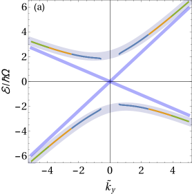
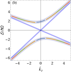
Figure 6: Cut of the quasi-energy spectrum with the section plane $k_{x}=0$ as a function of the pseudo-momentum $\widetilde{k}_{y}$ for (a) $E_{x}=5.5$ V/m, $E_{y}=2.6$ V/m, $q=-1.77$ ($\zeta_{x}>\zeta_{y}$), and (b) $E_{x}=2.6$ V/m, $E_{y}=5.5$ V/m, $q=0.87$ ($\zeta_{x}<\zeta_{y}$). The bands of allowed states are distinguished with different colors: blue for $r=1$, orange for $r=2$, green for $r=3$ and red for $r=4$. The light blue solid lines are sections of the Dirac cone. The section of the quasi-energy spectrum in the approximation where $r=\sqrt{a}$ is shown for reference as a solid gray line.

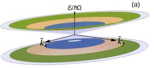
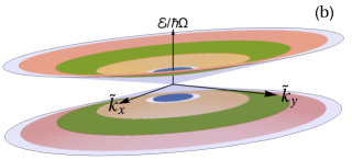
Figure 7: Quasi-energy spectrum as a function of the pseudo-momentum components $\widetilde{k}_{x}$ and $\widetilde{k}_{y}$ for (a) $E_{x}=5.5$ V/m, $E_{y}=2.6$ V/m, $q=-1.77$ ($\zeta_{x}>\zeta_{y}$), and (b) $E_{x}=2.6$ V/m, $E_{y}=5.5$ V/m, $q=0.87$ ($\zeta_{x}<\zeta_{y}$). The bands of allowed states are distinguished with different colors: blue for $r=1$, orange for $r=2$, green for $r=3$ and red for $r=4$.

These results clearly show that if $E_{x}>E_{y}$, the function $\Delta E(q)/2$ presents more domains that yield forbidden gaps close to the Dirac points than $E_{y}>E_{x}$. This strongly suggests that the shape and position of the gaps is strongly influenced by the relative orientation of the minor and major axes of the elliptical profiles of the radiation and the free-Weyl particle Dirac cone. If the major and minor axes of the ellipses arising from the Dirac cone are perpendicular to the major and minor axes of the ellipses of the electromagnetic profile, a gap at the Dirac point is more likely to form. Otherwise, if the ellipses are oriented in the same direction, gaps are more improbable. It is important to emphasize that this does not imply that the two ellipses necessarily have to have the the same proportions. Nevertheless, the only way to correctly predict the formation of a gap in the Dirac point is to determine if the value of $q$ falls inside one of the domains were $\Delta E>0$, as we discussed above.

III.2 Quasi-energy spectrum

The Hamiltonian in Schrödinger equation (6) is a periodic function of time, therefore the Floquet theorem must hold and, consequently, the wave function must be of the form

$$\boldsymbol{\Psi}(\boldsymbol{r},t)=\mathcal{N}\exp\left(-i\frac{\mathcal{E}t}{\hbar}\right)\boldsymbol{f}(\Omega t).$$ (31)

The phase $\mathcal{E}$ is usually termed the quasi-energy and $\boldsymbol{f}(\Omega t)=\boldsymbol{f}(\Omega t+2\pi)$ is a periodic function of time with the same period $T=2\pi/\Omega$ as the Hamiltonian. Using Eqs. (23) and (24) we can rearrange the Mathieu functions as

$$\mathcal{C}(a,q,\Omega t)-i\eta\mathcal{S}(a,q,\Omega t)=\exp[-i\eta r(a,q)\Omega t]f(\Omega t),$$ (32)

where $r(a,q)$ is purely rational and therefore $a_{r}=b_{r}$ as we discussed before. Substituting Eq. (32) into (26) and comparing with (31) we find the explicit expression for the quasi-energy

$$\frac{\mathcal{E}}{\hbar\Omega}=\frac{v_{t}k_{y}}{\Omega}+\eta r(a,q).$$ (33)

To better visualize the shape of the spectrum we may use $r\approx\sqrt{a}$ for $r\gg 1$ to approximate the quasi-energy. Using the definition of $a$ (21) and taking the limit for large quasi-momenta we get

$$\lim_{k_{x},k_{y}\rightarrow\infty}\mathcal{E}=\hbar v_{t}k_{y}+\hbar\sqrt{v_{x}^{2}k_{x}^{2}+v_{y}^{2}k_{y}^{2}}.$$ (34)

Hence, the quasi-energy spectrum asymptotically approaches the Dirac cone for large quasi-momentum values. This feature is clearly seen in Fig. 6. The light blue straight lines are the section of the Dirac cone cut by the $k_{x}=0$ plane and the solid gray lines are the quasi-energy spectrum in the approximation $r=\sqrt{a}$. The blue, orange, green and red lines correspond to the different bands arising from the exact expression of the quasi-energy (33). We readily confirm that both, the exact and the approximated quasi-energy spectrum lines, asymptotically come close to the Dirac cone. This is also seen in Fig. 7, where the full quasi-energy surface is shown and the Dirac cone is depicted as a light blue semi-transparent surface. The most striking characteristic of these plots is the formation of gaps. In Fig. 6 (a) a gap appears close to the Dirac point for $E_{x}=5.5$ V/m, $E_{y}=2.6$ V/m and $q=-1.77$. It is located inside the same region as the forbidden states in the dressed Dirac cone shown in Fig. 4 (a). In the full spectrum of Fig. 7 (a) this gap translates into a disc-shaped vacuum of states in the tip of the quasi-energy spectrum. Instead, for $E_{x}=2.6$ V/m, $E_{y}=5.5$ V/m and $q=0.87$ there is no gap formation close to the Dirac point, though, a ring-shaped gap appears around the tip of the quasi-energy spectrum as it is shown in Figs. 6 (b) and 7 (b). These results are consistent with the ones found for the dressed Dirac cones. Newly, the relative orientation of the minor and major axes of the radiation and the Dirac cone determine the location and structure of the gaps.

IV Conclusions

We have systematically investigated the wave function stability of charge carries in a Weyl Hamiltonian under an intense elliptically polarized electromagnetic radiation. To this end, we have worked out the time-dependent wave function from the Schrödinger equation in the limit of strong electric field (or long wavelength). We have proven that the stability properties of the wave functions are inherited from the Mathieu functions, in terms of which they are expressed. The analysis of the stability chart of the Mathieu functions projected onto the Dirac cones shows the formation of gaps of unstable states for certain domain regions of the quasi-momentum space. We have shown that the structure of the gaps strongly depends on the alignment between the minor and major axes of the elliptical profiles of the radiation and the Dirac cone of the free-Weyl particle spectrum. In summary, the formation of a gap at the Dirac point is more likely if the radiation and Dirac cone axes do not match, or are perpendicular. Otherwise, if the axes are aligned, ring-shaped gaps form for higher energies. The quasi-energy spectrum extracted from the phase of the wave function consistently reproduces the position and shapes of these gaps. Magnitude estimations of the electromagnetic fields and gap values were presented for the $8-Pmmn$ borophene phase.

V Acknowledgements

This work was supported by DCB UAM-A grant numbers 2232214 and 2232215, and UNAM DGAPA PAPIIT IN102717. V.G.I.S and J.C.S.S. acknowledge the total support from DGAPA-UNAM fellowship.

Appendix A

In this Appendix, we derive Eqs. (6) and (10) from the ansatz (7) and (9). We start from the Dirac equation (6) and applying the solution (7), we obtain Eq. (8), where

$$\mathbbm{H}(t)=\begin{pmatrix}\alpha_{\mathbf{k}}&\beta^{*}_{\mathbf{k}}\\ \beta_{\mathbf{k}}&\alpha_{\mathbf{k}}\end{pmatrix},$$ (35)

whose matrix elements are given by

$$\alpha_{\mathbf{k}}=\hbar v_{t}k_{y}-v_{t}eA_{y},$$ (36)

$$\beta_{\mathbf{k}}=\hbar(v_{x}k_{x}+iv_{y}k_{y})-e[v_{x}A_{x}+iv_{y}A_{y}].$$ (37)

In the previous equatins, the vector components $A_{x}$ and $A_{y}$ only depend on the time variable.

Now, we substitute Eq. (9) in Eq. (8), to get

$$\mathbbm{\widetilde{H}}(t)\bm{\chi}(t)=i\hbar\frac{d}{dt}\bm{\chi}(t),$$ (38)

where

$$\mathbbm{\widetilde{H}}(t)=\begin{pmatrix}0&\beta^{*}_{\mathbf{k}}\\ \beta_{\mathbf{k}}&0\end{pmatrix}.$$ (39)

From Eq. (38) we obtain

$$\frac{d^{2}}{dt^{2}}\bm{\chi}(t)+\frac{i}{\hbar}\left[\frac{d}{dt}\mathbbm{\widetilde{H}}(t)\right]\bm{\chi}(t)+\frac{1}{\hbar^{2}}\left[\mathbbm{\widetilde{H}}(t)\right]^{2}\bm{\chi}(t)=0,$$ (40)

where

$$\frac{d}{dt}\mathbbm{\widetilde{H}}(t)=-\hat{\bm{\sigma}}\cdot\frac{d\bm{S}}{dt}.$$ (41)

In the equations above we used the vectors $\hat{\bm{\sigma}}=(\hat{\sigma}_{x},\hat{\sigma}_{y})$ and $\bm{S}=e(v_{x}A_{x},v_{y}A_{y})$. Therefore, Eq. (40) can be reduced into

$$\frac{d^{2}}{dt^{2}}\bm{\chi}(t)+\mathbbm{F}(t)\bm{\chi}(t)=0,$$ (42)

with

$$\mathbbm{F}(t)=-\frac{i}{\hbar}\hat{\bm{\sigma}}\cdot\frac{d\bm{S}}{dt}+\frac{1}{\hbar^{2}}\left[\mathbbm{\widetilde{H}}(t)\right]^{2},$$ (43)

and

$$\left[\widetilde{\mathbbm{H}}(t)\right]^{2}=\left|\bm{\kappa}_{\bm{v}}-\bm{S}\right|^{2},$$ (44)

where $\boldsymbol{\kappa}_{\boldsymbol{v}}=\hbar(v_{x}k_{x},v_{y}k_{y})$.

Appendix B

To estimate the gap size, first, we calculate the value of the parameter $q$ from the Eq. (20), and subsequently use the expression López-Rodríguez and Naumis (2010); Champo and Naumis (2019)

$$\Delta_{r}=\hbar\Omega\sqrt{|b_{r}(q)-a_{r}(q)|},$$ (45)

where $a_{r}(q)$ and $b_{r}(q)$ for $r\in\mathbbm{Z}$ are the boundaries of a forbidden region as it is shown in Fig. 2.

For a microwave with frequency $\Omega=50$ GHz, we estimate the gap in the following cases: a) For $E_{x}=5.5$ V/m and $E_{y}=2.6$ V/m ( $\zeta_{x}>\zeta_{y}$), we find $q=-1.77$ and $\Delta^{L}_{3}=13.22\,\mu$ eV. b) For $E_{x}=2.6$ V/m and $E_{y}=5.5$ V/m ($\zeta_{x}<\zeta_{y}$), we find $q=0.87$ and $\Delta^{R}_{2}=19.45\,\mu$ eV.

References

- Novoselov et al. (2012) K. S. Novoselov, V. Fal, L. Colombo, P. Gellert, M. Schwab, K. Kim, et al., nature 490, 192 (2012).
- Peng et al. (2016) B. Peng, H. Zhang, H. Shao, Y. Xu, R. Zhang, and H. Zhu, Journal of Materials Chemistry C 4, 3592 (2016).
- Ferrari et al. (2015) A. C. Ferrari, F. Bonaccorso, V. Fal’Ko, K. S. Novoselov, S. Roche, P. Bøggild, S. Borini, F. H. Koppens, V. Palermo, N. Pugno, et al., Nanoscale 7, 4598 (2015).
- Naumis et al. (2017) G. G. Naumis, S. Barraza-Lopez, M. Oliva-Leyva, and H. Terrones, Reports on Progress in Physics 80, 096501 (2017).
- Geim (2009) A. K. Geim, science 324, 1530 (2009).
- Neto et al. (2009) A. C. Neto, F. Guinea, N. M. Peres, K. S. Novoselov, and A. K. Geim, Reviews of modern physics 81, 109 (2009).
- Oliva-Leyva and Naumis (2014) M. Oliva-Leyva and G. G. Naumis, Journal of Physics: Condensed Matter 26, 125302 (2014).
- Naumis and Roman-Taboada (2014) G. G. Naumis and P. Roman-Taboada, Physical Review B 89, 241404 (2014).
- Oliva-Leyva and Naumis (2015a) M. Oliva-Leyva and G. G. Naumis, Physics Letters A 379, 2645 (2015a).
- Oliva-Leyva and Naumis (2015b) M. Oliva-Leyva and G. G. Naumis, 2D Materials 2, 025001 (2015b).
- Oliva-Leyva and Naumis (2015c) M. Oliva-Leyva and G. G. Naumis, Journal of Physics: Condensed Matter 28, 025301 (2015c).
- Carrillo-Bastos and Naumis (2018) R. Carrillo-Bastos and G. G. Naumis, physica status solidi (RRL)–Rapid Research Letters 12, 1800072 (2018).
- Wehling et al. (2014) T. Wehling, A. M. Black-Schaffer, and A. V. Balatsky, Advances in Physics 63, 1 (2014).
- Jose and Datta (2013) D. Jose and A. Datta, Accounts of chemical research 47, 593 (2013).
- Liu et al. (2013) H. Liu, J. Gao, and J. Zhao, The Journal of Physical Chemistry C 117, 10353 (2013).
- Behera and Mukhopadhyay (2011) H. Behera and G. Mukhopadhyay, in AIP Conference Proceedings, Vol. 1349 (AIP, 2011) pp. 823–824.
- Zhang et al. (2016a) L. Zhang, P. Bampoulis, A. Rudenko, Q. v. Yao, A. Van Houselt, B. Poelsema, M. Katsnelson, and H. Zandvliet, Physical review letters 116, 256804 (2016a).
- Zhu et al. (2015) F.-f. Zhu, W.-j. Chen, Y. Xu, C.-l. Gao, D.-d. Guan, C.-h. Liu, D. Qian, S.-C. Zhang, and J.-f. Jia, Nature materials 14, 1020 (2015).
- Chen et al. (2016) X. Chen, R. Meng, J. Jiang, Q. Liang, Q. Yang, C. Tan, X. Sun, S. Zhang, and T. Ren, Physical Chemistry Chemical Physics 18, 16302 (2016).
- Soltan-Panahi et al. (2011) P. Soltan-Panahi, J. Struck, P. Hauke, A. Bick, W. Plenkers, G. Meineke, C. Becker, P. Windpassinger, M. Lewenstein, and K. Sengstock, Nature Physics 7, 434 (2011).
- Gomes et al. (2012) K. K. Gomes, W. Mar, W. Ko, F. Guinea, and H. C. Manoharan, Nature 483, 306 (2012).
- Zhang et al. (2017) Z. Zhang, E. S. Penev, and B. I. Yakobson, Chemical Society Reviews 46, 6746 (2017).
- Boustani (1997) I. Boustani, Surface Science 370, 355 (1997).
- Mannix et al. (2015) A. J. Mannix, X.-F. Zhou, B. Kiraly, J. D. Wood, D. Alducin, B. D. Myers, X. Liu, B. L. Fisher, U. Santiago, J. R. Guest, M. J. Yacaman, A. Ponce, A. R. Oganov, M. C. Hersam, and N. P. Guisinger, Science 350, 1513 (2015), https://science.sciencemag.org/content/350/6267/1513.full.pdf .
- Verma et al. (2017) S. Verma, A. Mawrie, and T. K. Ghosh, Physical Review B 96, 155418 (2017).
- Champo and Naumis (2019) A. E. Champo and G. G. Naumis, Physical Review B 99, 1 (2019).
- Zhang et al. (2016b) L. Zhang, Y. Zhou, L. Guo, W. Zhao, A. Barnes, H.-T. Zhang, C. Eaton, Y. Zheng, M. Brahlek, H. F. Haneef, et al., Nature materials 15, 204 (2016b).
- López-Rodríguez and Naumis (2010) F. López-Rodríguez and G. Naumis, Philosophical Magazine 90, 2977 (2010).
- Higuchi et al. (2017) T. Higuchi, C. Heide, K. Ullmann, H. B. Weber, and P. Hommelhoff, Nature 550, 224 (2017).
- López-Rodríguez and Naumis (2008) F. López-Rodríguez and G. Naumis, Physical Review B 78, 201406 (2008).
- Kibis (2010) O. Kibis, Physical Review B 81, 165433 (2010).
- Kristinsson et al. (2016a) K. Kristinsson, O. V. Kibis, S. Morina, and I. A. Shelykh, Scientific reports 6, 20082 (2016a).
- Oliva-Leyva and Naumis (2016) M. Oliva-Leyva and G. G. Naumis, Physical Review B 93, 035439 (2016).
- Kristinsson et al. (2016b) K. Kristinsson, O. V. Kibis, S. Morina, and I. A. Shelykh, Scientific Reports 6, 20082 EP (2016b).
- Kibis et al. (2017) O. Kibis, K. Dini, I. Iorsh, and I. Shelykh, Physical Review B 95, 125401 (2017).
- Islam and Jayannavar (2017) S. K. Islam and A. M. Jayannavar, Physical Review B 96, 1 (2017).
- Zabolotskiy and Lozovik (2016) A. D. Zabolotskiy and Y. E. Lozovik, Physical Review B 94, 1 (2016).
- Magnus and Winkler (2013) W. Magnus and S. Winkler, Hill’s equation (Courier Corporation, 2013).
- Urwin and Arscott (1970) K. M. Urwin and F. Arscott, Proceedings of the Royal Society of Edinburgh Section A: Mathematics 69, 28 (1970).
- Ziener et al. (2012) C. Ziener, M. Rückl, T. Kampf, W. Bauer, and H. Schlemmer, Journal of Computational and Applied Mathematics 236, 4513 (2012).
- Aldrovandi and Ferreira (1980) R. Aldrovandi and P. L. Ferreira, American Journal of Physics 48, 660 (1980).
- Baker and Blackburn (2005) G. L. Baker and J. A. Blackburn, The pendulum: a case study in physics (Oxford University Press, 2005).
- McLachlan (1951) N. W. McLachlan, (1951).
- Landau (1946) L. D. Landau, Zh. Eksp. Teor. Fiz. 10, 25 (1946).
- Davydov (1980) A. S. Davydov, Théorie du solide (Editions Mir, 1980).