Dynamic winding number for exploring band topology

Abstract

Topological invariants play a key role in the characterization of topological states. Due to the existence of exceptional points, it is a great challenge to detect topological invariants in non-Hermitian systems. We put forward a dynamic winding number, the winding of realistic observables in long-time average, for exploring band topology in both Hermitian and non-Hermitian two-band models via a unified approach. We build a concrete relation between dynamic winding numbers and conventional topological invariants. In one-dimension, the dynamical winding number directly gives the conventional winding number. In two-dimension, the Chern number relates to the weighted sum of dynamic winding numbers of all phase singularity points. This work opens a new avenue to measure topological invariants not requesting any prior knowledge of system topology via time-averaged spin textures.

Introduction. Topological invariant, a global quantity defined with static Bloch functions, has been widely used for classifying and characterizing topological states of matters, including insulators, superconductors, semimetals and waveguides etc Qi and Zhang (2011); Bernevig and Hughes (2013); Ando (2013); Chiu et al. (2016); Lv et al. (2017); Ozawa et al. (2019). Nontrivial topological invariants attribute to novel topological effects, such as winding number for quantized geometric phase Cao et al. (2018); Yin et al. (2018), and Chern number for integer Hall effect Thouless et al. (1982); Hatsugai (1993) and Thouless pumping Thouless (1983); Ke et al. (2016); Lohse et al. (2018). Measuring topological invariants provide undoubted evidence of topological states, beneficial for precision measurement Klitzing et al. (1980); Cooper and Rey (2015), error-resistant spintronics Nayak et al. (2008); Pesin and MacDonald (2012) and quantum computing Haldane (2017); Lian et al. (2018).

Most existed methods to measure topological invariants are based on adiabatic band sweeping Atala et al. (2013); Jotzu et al. (2014); Aidelsburger et al. (2015); Fläschner et al. (2016); Hu et al. (2019). However, these methods do not work well for imperfect initial states and small energy gaps and become invalid for non-Hermitian systems. In recent, topological invariants have been measured via linking numbers and band-inversion surfaces in quench dynamics Wang et al. (2017); Qiu et al. (2018); Sun et al. (2018, 2018); Zhang et al. (2018); Tarnowski et al. (2019); Zhang et al. (2019). However, these quench schemes request prior knowledge of topology before and after quench.

As non-Hermitian systems may exhibit complex spectra and exceptional points (EPs) Heiss (2012); Hu et al. (2017); Hassan et al. (2017), their topological states have stimulated extensive interests Esaki et al. (2011); Liang and Huang (2013); Malzard et al. (2015); Lee (2016); Leykam et al. (2017); Rakovszky et al. (2017); Lieu (2018); Alvarez et al. (2018); Yoshida et al. (2018); Zhou and Gong (2018); Chen and Zhai (2018); Yoshida et al. (2019a); S. Borgnia et al. (2019); Yoshida et al. (2019b).Conventional topological invariants such as winding number and Chern number have been generalized to non-Hermitian systems Lee (2016); Yin et al. (2018); Shen et al. (2018), and new topological invariants such as vorticity have been introduced Ghatak and Das (2019). Due to the EPs, the winding number in non-Hermitian systems may take half-integers Lee (2016); Yin et al. (2018); Jiang et al. (2018); Jin and Song (2019). Besides, non-Bloch definition of Chern number strictly gives the numbers of chiral edge modes Yao and Wang (2018); Yao et al. (2018); Ghatak et al. (2019). How to measure these topological invariants is more challenging than that in Hermitian systems. For an example, the Hall conductivity is no longer quantized despite being classified as a Chern insulator based on non-Hermitian topological band theory Philip et al. (2018); Chen and Zhai (2018). In one-dimension, the winding number in a non-Hermitian system has been determined via the mean displacement in long-time quantum walk Rudner and Levitov (2009); Zeuner et al. (2015), but it does not works for measuring Chern numbers and half-integer winding numbers. One may ask, is there a unified dynamic approach for measuring topological invariants in both Hermitian and non-Hermitian systems?

In this Letter, we study a generic two-band model which supports nontrivial topological invariants in both Hermitian and non-Hermitian regions. We define a dynamic winding number (DWN) for the time-averaged spin textures, which is robust against various initial states. In one-dimension, we prove that the DWNs directly gives the conventional winding numbers in both chiral- and non-chiral-symmetric systems. In two-dimension, the Chern number relates to the weighted sum of DWNs around all singularity points (SPs), where the weight is $+1$ for the north pole and $-1$ for the south pole. When the system change from Hermitian to non-Hermitian, each singularity point will split into two EPs (which are also SPs), the Chern number can still be extracted via the DWNs of all EPs. Without requesting any prior knowledge of their topology, our approach provides a general guidance for measuring topological invariants in both Hermitian and non-Hermitian systems.

Dynamic winding number. We consider a general two-band model in $d-$dimension. The Hamiltonian in momentum space is composed of three Pauli matrices,

$$H(\bm{k})=h_{x}(\bm{k})\sigma_{x}+h_{y}(\bm{k})\sigma_{y}+h_{z}(\bm{k})\sigma_{z}.$$ (1)

Here, $\bm{k}$ is the quasi-momentum, $h_{x(y,z)}$ are periodic functions of $\bm{k}$. The Hamiltonian could be Hermitian $H^{\dagger}=H$ or non-Hermitian $H^{\dagger}\neq H$. Then, the right and left eigenvectors are respectively given by $H(\bm{k})|\varphi_{\mu}\rangle=\varepsilon_{{\mu}}|\varphi_{\mu}\rangle$ $(H^{\dagger}(\bm{k})|\chi_{\mu}\rangle=\varepsilon^{*}_{{\mu}}|\chi_{\mu}\rangle)$, where $\mu=\pm$, and $\varepsilon_{{\pm}}=\pm(h_{x}^{2}+h_{y}^{2}+h_{z}^{2})^{1/2}$ are the eigenvalues. For Hermitian systems, $|\varphi_{\mu}\rangle=|\chi_{\mu}\rangle$ and $\varepsilon_{\mu}=\varepsilon_{\mu}^{*}$. For non-Hermitian systems, neither the eigenstates $|\varphi_{\mu}\rangle$ nor $\langle\chi_{\mu}|$ are orthogonal. We adopt biorthogonal vectors which fulfil $\langle\chi_{\nu}|\varphi_{\mu}\rangle=\delta_{\nu,\mu}$ and $\sum_{{\mu}}|\varphi_{\mu}\rangle\langle\chi_{\mu}|=1$ by normalizing $|\varphi_{\mu}\rangle=|\varphi_{\mu}\rangle/N_{\mu}$ and $\langle\chi_{\mu}|=\langle\chi_{\mu}|/N_{\mu}$ with $N_{\mu}=\sqrt{{\langle\chi_{\mu}|\varphi_{\mu}\rangle}}$.

For an arbitrary initial state $|\psi_{\bm{k}}(0)\rangle=\sum_{\mu}c_{{\mu}}|\varphi_{\mu}\rangle$ and its associated state $\langle\tilde{\psi}_{\bm{k}}(0)|=\sum_{\mu}c_{{\mu}}^{*}\langle\chi_{\mu}|$, the time-evolution of $|\psi_{\bm{k}}(t)\rangle$ and $\langle\tilde{\psi}_{\bm{k}}(t)|$ respectively satisfy $|\psi_{\bm{k}}(t)\rangle=\sum_{\mu}c_{\mu}e^{-i\varepsilon_{{\mu}}t}|\varphi_{\mu}\rangle$ and $\langle\tilde{\psi}_{\bm{k}}(t)|=\sum_{\mu}c_{{\mu}}^{*}e^{i\varepsilon_{\mu}^{*}t}\langle\chi_{\mu}|$. According to the biorthogonal quantum mechanics Brody (2013), the spin textures are given by the expectation values of Pauli matrices, $\langle\sigma_{j}(\bm{k},t)\rangle={\langle\tilde{\psi}_{\bm{k}}(t)|\sigma_{j}|\psi_{\bm{k}}(t)\rangle}/{\langle\tilde{\psi}_{\bm{k}}(t)|\psi_{\bm{k}}(t)\rangle}$, where $j\in{x,y,z}$. We are interesting in its long-time average, $\overline{\sigma_{j}}(\bm{k})=\lim_{T\rightarrow\infty}\frac{1}{T}\int_{0}^{T}\langle\sigma_{j}(\bm{k},t)\rangle dt$. As the quasimomentum continuously varies, $(\overline{\sigma_{i}},\overline{\sigma_{j}})$ will form a trajectory in the polarization plane. The DWN of the spin vector $(\overline{\sigma_{i}},\overline{\sigma_{j}})$ is defined as

$$w_{d}=\frac{1}{2\pi}\oint_{S}\partial_{\bm{k}}\eta_{ji}(\bm{k})d\bm{k},$$ (2)

where $S$ is a close loop in parameter space $\bm{k}$, and dynamical azimuthal angle $\eta_{ji}(\bm{k})=\arctan[{\overline{\sigma_{j}}(\bm{k})}/{\overline{\sigma_{i}}(\bm{k})}]$. It is easy to prove that the DWN is convergent to the equilibrium azimuthal angle,

$$\eta_{ji}=\phi_{ji}\equiv\arctan\left[h_{j}(\bm{k})/h_{i}(\bm{k})\right],$$ (3)

if $|c_{+}|^{2}\neq|c_{-}|^{2}$ for Hermitian systems and $|c_{+}|^{2}\neq 0\bigcap|c_{-}|^{2}\neq 0$ for non-Hermitian systems Sup . For Hermitian systems, the DWN can be directly probed by the long-time average of spin textures. For non-Hermitian systems, $\eta_{ji}$ is a complex angle which cannot be directly observed. This problem can be fixed by decomposing the azimuthal angle into real and imaginary parts. We find that only the real part of $\eta_{ji}$ contributes to the DWN and it satisfies,

$$\Re(\eta_{ji})=\frac{1}{2}(\phi_{ji}^{RR}+\phi_{ji}^{LL})+n\frac{\pi}{2},$$ (4)

where $\phi_{ji}^{RR}=\arctan\big{(}{\overline{\langle\psi_{\bm{k}}|\sigma_{j}|\psi_{\bm{k}}\rangle}}/{\overline{\langle\psi_{\bm{k}}|\sigma_{i}|\psi_{\bm{k}}\rangle}}\big{)}$ and $\phi_{ji}^{LL}=\arctan\big{(}{\overline{\langle\tilde{\psi}_{\bm{k}}|\sigma_{j}|\tilde{\psi}_{\bm{k}}\rangle}}/{\overline{\langle\tilde{\psi}_{\bm{k}}|\sigma_{i}|\tilde{\psi}_{\bm{k}}\rangle}}\big{)}$ are both real Sup , $\Re(\eta_{ji})$ represents the real part of $\eta_{ji}$. Thus we have $w_{d}=\frac{1}{2}(w_{d}^{RR}+w_{d}^{LL})$, where $w_{d}^{\tau}=\frac{1}{2\pi}\oint_{S}\partial_{\bm{k}}\phi_{jl}^{\tau}d\bm{k}$, $\tau\in RR,LL$. This means that the DWN can also be observed by the time-evolution of left-left and right-right spin textures whose dynamics are respectively governed by $\hat{H}$ and $\hat{H}^{\dagger}$. In the following, we show how to utilize the DWN to uncover the topology in both Hermitian and non-Hermitian systems.

Connection between conventional winding number and dynamic winding number. In one-dimension, if $h_{z}=0$, the Hamiltonian (1) has chiral symmetry $\Gamma H(k)\Gamma=-H(k)$ with $\Gamma=i\sigma_{x}\sigma_{y}$ and $\bm{k}\rightarrow k$. The conventional winding number $w_{\pm}$ for the Hamiltonian (1) reads as,

$$w_{\pm}=\frac{1}{2\pi}\oint_{S}dk\frac{h_{x}\partial_{k}h_{y}-h_{y}\partial_{k}h_{x}}{(\varepsilon_{{\pm}})^{2}},$$ (5)

which associates with the Zak phase. According to Eqs. (2) and (5), one can find that $w_{\pm}=w_{d}$.

If $h_{z}\neq 0$, the Hamiltonian (1) breaks the chiral symmetry. The winding numbers $w_{\pm}$ can be given as,

$$w_{\pm}=\frac{1}{2\pi}\oint_{S}dk\frac{h_{x}\partial_{k}h_{y}-h_{y}\partial_{k}h_{x}}{\varepsilon_{{\pm}}(\varepsilon_{{\pm}}-h_{z})}.$$ (6)

Unlike the systems with chiral symmetry, the conventional winding number for each band is not a quantized number, which indicates that $w_{\pm}$ is no longer a topological invariant. However, the sum of two conventional winding numbers,

$$w_{t}=w_{+}+w_{-}=\frac{1}{\pi}\oint_{S}dk\frac{h_{x}\partial_{k}h_{y}-h_{y}\partial_{k}h_{x}}{h_{x}^{2}+h_{y}^{2}},$$ (7)

relates to the dynamic winding number via $w_{t}=2w_{d}$ and thus it can be used as a topological invariant.

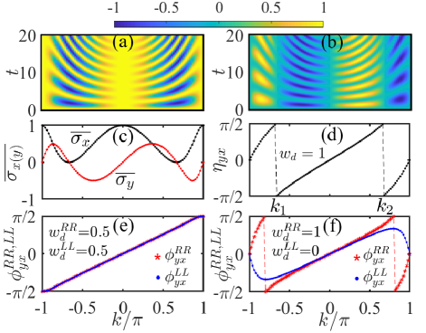
Figure 1: Extract conventional winding number via dynamic winding number. Hermitian case: (a) and (b) respectively show the time-evolution of the spin textures $\langle\sigma_{x}\rangle$ and $\langle\sigma_{y}\rangle$, (c) time-averaged spin textures $\overline{\sigma_{x}}$ (black line) and $\overline{\sigma_{y}}$ (red line) as a function of $k$, and (d) the dynamical azimuthal angle $\eta_{yx}$ as a function of $k$. In which, $k_{1}$ and $k_{2}$ are discontinuity points. Non-Hermitian case: $\phi_{yx}^{RR}$ and $\phi_{yx}^{LL}$ as a function of $k$ for (e) chiral-symmetric system with $h_{z}=0$ and (f) non-chiral-symmetric system with $h_{z}=0.5$.

As an example, we consider a system with $h_{x}=J_{0}+J_{1}\cos(k)$, $h_{y}=J_{1}\sin(k)-i\delta$ and $h_{z}=0$. In the Hermitian case, the parameters are chosen as $\delta=0$ and $J_{1}=1$. The conventional winding number $w_{\pm}=1$ for $|J_{0}|<J_{1}$, and $w_{\pm}=0$ for $|J_{0}|>J_{1}$. We first calculate the time-evolution of $\langle\sigma_{x(y)}(k,t)\rangle$ and their long-time average with $J_{0}=0.5J_{1}$, see Figs. 1(a)-(c). The spin textures $\langle\sigma_{x(y)}(k,t)\rangle$ oscillate with a momentum-dependent period $\widetilde{t}_{k}=\pi/|\varepsilon_{\mu}|$, and their long-time averages $\overline{\sigma_{x(y)}}$ depend on quasi-momentum, see the black and red lines in Fig. 1 (c). With $\overline{\sigma_{x}}$ and $\overline{\sigma_{y}}$, we calculate $\eta_{yx}$ as a function of $k$ in Fig. 1(d), where two discontinuity points $k_{1}$ and $k_{2}$ appear. The DWN can be obtained via the integral of piecewise function,

$$w_{d} = \frac{1}{2\pi}\big{(}\int_{-\pi}^{k_{1}}\partial_{k}\eta_{yx}dk+\int_{k_{1}}^{k_{2}}\partial_{k}\eta_{yx}dk+\int_{k_{2}}^{\pi}\partial_{k}\eta_{yx}dk\big{)}.$$

We find that the DWN is equal to $1$, the same as the conventional winding number $w_{\pm}$.

When $\delta\neq 0$, the system becomes non-Hermitian and one always needs to measure both $\phi_{ji}^{RR}$ and $\phi_{ji}^{LL}$ to extract the DWN. For a chiral-symmetric system (whose parameters are given as $J_{0}=J_{1}=1$, $\delta=0.3$, $h_{z}=0$ and $w_{\pm}=1/2$), the two dynamic azimuthal angles $\phi_{ji}^{RR}=\phi_{ji}^{LL}$, and $w_{d}^{RR}=w_{d}^{LL}=\frac{1}{2}$, see in Fig. 1(e). It means that we only need to measure $\phi_{ji}^{RR}$ or $\phi_{ji}^{LL}$ in experiments. For a non-chiral-symmetric system (whose parameters are given as $J_{0}=J_{1}=1$, $\delta=0.3$, $h_{z}=0.5$, and $w_{t}=1$), we find $\phi_{ji}^{RR}\neq\phi_{ji}^{LL}$, and $w_{d}^{RR}=1,w_{d}^{LL}=0$, see Fig. 1(f). Nevertheless, the conventional winding number can be obtain by measuring the $w_{d}=(w_{d}^{RR}+w_{d}^{LL})/2$ in both chiral and non-chiral symmetric systems.

Connection between Chern number and dynamic winding number. By generalizing the concept of gapped band structures from Hermitian to non-Hermitian systems, the Chern number for an energy separable band can be constructed in a similar way Shen et al. (2018). In contrast to Hermitian systems, there are left-right, right-right, left-left, right-left Chern numbers in non-Hermitian systems, dependent on the definitions of Berry connection, $A_{\bm{k}}^{LR}=i\langle\chi_{\mu}|\partial_{\bm{k}}|\varphi_{\mu}\rangle$, $A_{\bm{k}}^{RR}=i\langle\varphi_{\mu}|\partial_{\bm{k}}|\varphi_{\mu}\rangle$, $A_{\bm{k}}^{LL}=i\langle\chi_{\mu}|\partial_{\bm{k}}|\chi_{\mu}\rangle$, and $A_{\bm{k}}^{RL}=i\langle\varphi_{\mu}|\partial_{\bm{k}}|\chi_{\mu}\rangle$. Although the corresponding Berry curvatures are locally different quantities, but the four kinds of Chern numbers are the same Shen et al. (2018). Here, we only focus on analyzing the Chern number defined with left-right Berry connection $A_{\bm{k}}^{LR}=i\langle\chi_{\mu}|\partial_{\bm{k}}|\varphi_{\mu}\rangle$, which naturely reduces the Chern number in Hermitian systems as $|\varphi_{\mu}\rangle=|\chi_{\mu}\rangle$.

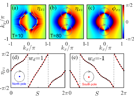
Figure 2: Topologically nontrivial phase with Chern number $C=1$. (a) and (b) respectively show $\eta_{xz}(k_{x},k_{y})$ obtained in the evolved time $T=10$ and $T=80$, and (c) displays $\phi_{xz}(k_{x},k_{y})$. (d) and (e) show how $\eta_{xz}$ (black dots) and $\phi_{xz}$ (red line) change along the trajectory around the north and south poles in (b) and (c), respectively.

We map the Hamiltonian to a normalized vector, $\vec{n}(\bm{k})=(\sin(\theta_{i})\cos(\phi_{jl}),\sin(\theta_{i})\sin(\phi_{jl}),\cos(\theta_{i}))$, which reduces a Bloch vector in Hermitian systems. Here, $\theta_{i}$ denotes the angle between the vector and the axis-$i$, and $\phi_{jl}$ denotes the equilibrium azimuthal angle in the $j-l$ plane. The reference axis is free to choose without affecting the validity of the dynamic approach. Then, the left and right eigenstates for the low-energy band are given as

$$\langle\chi_{-}(\theta_{i},\phi_{jl})|=\begin{pmatrix}-e^{i\phi_{jl}/2}\cos(\frac{\theta_{i}}{2}),e^{-i\phi_{jl}/2}\sin(\frac{\theta_{i}}{2})\end{pmatrix},$$

$$|\varphi_{-}(\theta_{i},\phi_{jl})\rangle=\begin{pmatrix}-e^{-i\phi_{jl}/2}\cos(\frac{\theta_{i}}{2})\\ e^{i\phi_{jl}/2}\sin(\frac{\theta_{i}}{2})\end{pmatrix}.$$ (8)

The right and left eigenstates have a phase singularity at $\vec{n}(\bm{k})=(0,0,\pm 1)$, in which $+$ and $-$ respectively correspond to north and south poles. In the parameter space $(k_{x},k_{y})$, the location $\bm{k}_{0}$ of the poles satisfy $h_{j}(\bm{k}_{0})^{2}+h_{l}(\bm{k}_{0})^{2}=0$. The left-right Berry connection ${A}_{k_{x(y)}}^{LR}$ of the low-energy band are given by

$${A}_{k_{x(y)}}^{LR}=i\langle\chi_{-}|\partial_{k_{x(y)}}|\varphi_{-}\rangle=\frac{\cos(\theta_{i})}{2}\frac{\partial\phi_{jl}}{\partial_{k_{x(y)}}}.$$

We discreterize the parameter space $(k_{x},k_{y})$ by $N\times M$ mesh grids in the first Briliouin zone Fukui et al. (2005). For each grid, a direct application of the two-dimensional Stokes theorem implies Asbóth et al. (2016)

$$C^{LR}=\frac{1}{2\pi}\sum\limits_{l_{x}=1}^{N}\sum\limits_{l_{y}=1}^{M}\oint_{S_{l_{x},l_{y}}}(A_{k_{x}}dk_{x}+A_{k_{y}}dk_{y}),$$ (9)

where $S_{l_{x},l_{y}}$ represents the clockwise path integration of the $(l_{x},l_{y})$ grid. We find that the Chern number is determined by the winding numbers for all SPs, where $\cos(\theta_{i})=h_{i}(\bm{k_{0}})/|\vec{h}(\bm{k_{0}})|=sgn(\Re[h_{i}(\bm{k_{0}})])=1$ for the north SPs and $\cos(\theta_{i})=-1$ for the south SPs, $\Re[h_{i}(\bm{k_{0}})]$ represents the real part of $h_{i}(\bm{k_{0}})$, and $\vec{h}=(h_{x},h_{y},h_{z})$. At last, we can deduce the left-right Chern number as

$$C^{LR}=\frac{1}{2}\sum\limits_{\bm{k}_{0}\in\rm{SPs}}sgn(\Re[h_{i}(\bm{k_{0}})])w_{d}(\bm{k}_{0}),$$ (10)

where $w_{d}(\bm{k}_{0})$ is the DWN for the SP at ${\bm{k}}_{0}$ Sup . In non-Hermitian case, $w_{d}(\bm{k}_{0})$ is relevant to two real angles $\phi_{jl}^{RR}$ and $\phi_{jl}^{LL}$, which can be respectively extracted via right-right spin textures $\langle{\psi}_{\bm{k}}(t)|\sigma_{j(l)}|\psi_{\bm{k}}(t)\rangle$ and left-left spin textures $\langle\tilde{\psi}_{\bm{k}}(t)|\sigma_{j(l)}|\tilde{\psi}_{\bm{k}}(t)\rangle$.

As an example, we consider $h_{x}=J_{x}\sin(k_{x})$, $h_{y}=J_{y}\sin(k_{y})$ and $h_{z}=m_{z}-J_{z}\cos(k_{x})-J_{z}\cos(k_{y})-i\delta$ Sup . Here, $J_{x(y,z)}$ denote spin-orbit coupling parameters, $m_{z}$ is the effective magnetization, and $\delta$ is a gain or loss strength. When $\delta=0$, the system is a quantum anomalous Hall model Liu et al. (2014), which has been realized in recent experiments Chang et al. (2013); Sun et al. (2018). In the Hermitian case ($J_{x(y,z)}=1,\ m_{z}=1,\ \delta=0$), the north and south poles in the parameter space $(k_{x},k_{y})$ can be determined as following. Since the poles are related to the chosen axis, we select $\theta=\theta_{y}=\arccos(h_{y}/|\vec{h}(\bm{k})|)$ and $\phi=\phi_{xz}=\arctan(h_{x}/h_{z})$. However, the validity of our dynamic approach is independent on the choice of reference axis Sup . In the parameter space $(k_{x},k_{y})$, by solving $h_{x}^{2}+h_{z}^{2}=0$, we find that the north and south poles locate at $\bm{k}_{0}=(k_{x},k_{y})=(0,\pm\pi/2)$.Then, we need to extract the DWN around the two poles. We randomly choose an initial state $|\psi_{\bm{k}}(0)\rangle=\sum_{\mu}c_{{\mu}}|\varphi_{\mu}\rangle$ with $|c_{+}|^{2}>|c_{-}|^{2}$ and calculate the spin textures $\left\langle\sigma_{x}(\bm{k},t)\right\rangle$ and $\left\langle\sigma_{z}(\bm{k},t)\right\rangle$. The dynamical azimuthal angle $\eta_{xz}(\bm{k})$ can be extracted via long-time average values $\overline{\sigma_{x(z)}}(\bm{k})$, see Figs. 2(a) and 2(b). We also calculate the equilibrium azimuthal angle $\phi_{xz}(\bm{k})$ via the eigenstates, see Fig. 2(c). The difference between $\eta_{xz}(\bm{k})$ and $\phi_{xz}(\bm{k})$ gradually disappears with the increase of total time $T$. Thus we can obtain the DWNs for the north and south poles via integrating the gradient of $\eta_{xz}(\bm{k})$ in Fig. 2(d) and 2(e), respectively. The DWNs for the north and south poles are respectively given as $w_{d}=\pm 1$. Applying Eq. (10), one can obtain the Chern number as $1$, which is consistent with the one calculated via integrating the static Berry curvature over the whole in the parameter space $(k_{x},k_{y})$.

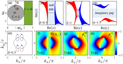
Figure 3: (a) Topological phase diagram. (b)-(d) Energies of bulk bands (red and blue regions) and edge mode (black line) in the complex-energy plane, corresponding to the parameter points $b$-$d$ in (a). (e) North EPs (blue dots) and south EPs (red dots) with $\delta=0.5$. (f)-(h) Dynamic azimuthal angles $\Re[\eta_{xz}(k_{x},k_{y})]$, $\phi_{xz}^{RR}(k_{x},k_{y})$ and $\phi_{xz}^{LL}(k_{x},k_{y})$, which are defined with left-right, right-right and left-left spin textures in the evolved time $T=80$.

In the more generalized case, we first show the topological phase diagram in the parameter plane ($m_{z},\delta$) by setting $J_{x(y,z)}=1$, see Fig. 3(a). The Chern numbers of the first band are $C=0$ and $1$ in the green and grey regions, and not well defined in the white region. The boundaries satisfy $(m_{z}-1)^{2}+\delta^{2}<1$ for the gray region and $m_{z}>2$ for the green region. Varying $\delta$ along the dashed red arrow, in Figs. 3(b)–(d) we explore the correspondence between the Chern number and energy modes under open boundary condition, corresponding to the parameter points $b$-$d$. For the topological nontrivial phase, one can see that the complex bulk bands are still gapped and the edge-state modes are still preserved in the real energy axis, see Fig. 3(b). Now we consider $\delta=0.5$ and keep other parameters the same as those in Fig. 2(b). We find that the two poles in Hermitian case are split into four EPs, see Fig. 3(e). The blue and red points represent north and south EPs, respectively. In Figs. 3(f), we give $\Re(\eta_{xz})$ in parameter space $(k_{x},k_{y})$, and the DWNs can be obtain by integral of the dynamic azimuthal-angle gradient along the trajectory enclosing the north and south EPs. Here, the DWNs for the north and south EPs are $w_{d}=1/2$ and $-1/2$, respectively. Although the SPs are doubled, as each DWN is reduced by half, the Chern number keep unchanged. For completeness, we also show the dynamic azimuthal angles defined with the right-right and left-left spin textures, see Fig. 3(g) and 3(h) . The dynamic azimuthal angles are quite different from each other, corresponding to $\phi_{xz}^{RR}$ and $\phi_{xz}^{LL}$, respectively. Nevertheless, the north and south EPs are the same as those in the Fig. 3(e). Around an EP, one can extract the right-right and left-left DWN $w_{d}^{RR}$ and $w_{d}^{LL}$, which satisfy $w_{d}=\frac{1}{2}(w_{d}^{RR}+w_{d}^{LL})$. One important thing is that the $\phi_{xz}^{RR}$ and $\phi_{xz}^{LL}$ defined with the real left-left and right-right spin textures are accessible in experimental measurements.

In addition, our approach can also extract larger Chern numbers without extra efforts Sup , which is very hard to access by adiabatic band sweeping.

Conclusions and Discussions. We put forward a new concept of dynamic winding number (DWN) and uncover its connection to conventional topological invariants in both Hermitian and non-Hermitian models. Given a time-averaged spin texture in the parameter space, a DWN is given by a loop integral of the dynamic azimuthal-angle gradient enclosing a single singularity point. We find that, (i) the conventional winding numbers in one-dimensional systems can be directly given by the corresponding DWNs, and (ii) the Chern numbers in two-dimensional systems relates to the weighted sum of all corresponding DWNs. Our scheme has two main advantages. Firstly, in contrast to the quench schemes via measuring linking numbers Wang et al. (2017); Tarnowski et al. (2019) and band-inversion surfaces Zhang et al. (2018); Sun et al. (2018), which request prior knowledge of topology before and after quench, our scheme does not request any prior knowledge. Secondly, our scheme can be used to measure half-integer winding numbers in non-Hermitian one-dimensional systems, which can not be measured via previous methods.

Our scheme is readily realized in various systems, ranging from cold atoms in optical lattices, optical waveguide arrays, to optomechanical devices. In Supplementary Material Sup , we provide more details about the experimental realization of our scheme via cold atoms and optical waveguide arrays. In future, it would be interesting to extend our scheme to measure topological invariants in high-dimensional systems, multi-band systems, periodically driven systems and disordered systems.

Supplemental Material

S1 S1. Convergence of dynamic winding number

According to Eq.(2) in the main text, it seems that the definition of dynamic winding number depends on the initial state, and it is unclear whether such number is convergent in the long time. Here, we prove that the initial state can be rather general and the dynamic winding number is convergent. The time-average of $\langle\sigma_{j}\rangle$ is given as

$$\overline{\sigma_{j}}=\lim_{T\rightarrow\infty}\frac{1}{T}\int_{0}^{T}\frac{\sum_{\mu,\mu^{\prime}}c_{\mu}c_{\mu^{\prime}}^{*}e^{-i(\varepsilon_{\mu}-\varepsilon_{\mu^{\prime}}^{*})t}\langle\chi_{\mu^{\prime}}|\sigma_{j}|\varphi_{\mu}\rangle}{\sum_{\mu}|c_{\mu}|^{2}e^{-i(\varepsilon_{\mu}-\varepsilon_{\mu}^{*})t}}dt.$$ (S1)

For Hermitian systems, $\varepsilon_{\mu}=\varepsilon_{\mu}^{*}$, and the periodic terms vanish in the long time average and only the diagonal terms preserve. The above equation can be simplified as

$$\overline{\sigma_{j}}=\sum\limits_{\mu}|c_{\mu}|^{2}\langle\chi_{\mu}|\sigma_{j}|\varphi_{\mu}\rangle=\big{(}|c_{+}|^{2}-|c_{-}|^{2}\big{)}\frac{h_{j}}{\varepsilon_{+}}$$ (S2)

For the non-Hermitian systems, we assume that the eigenenergy $\varepsilon_{\mu}=\mu(A+iB)$, where $A$ and $B$ are real numbers. When $B>0$, Eq. (S1) is approximately given as

$$\overline{\sigma_{j}} = \langle\chi_{+}|\sigma_{j}|\varphi_{+}\rangle=\frac{h_{j}}{\varepsilon_{+}}.$$ (S3)

Similarly, when $B<0$, Eq. (S1) is approximately given as

$$\overline{\sigma_{j}} = \langle\chi_{-}|\sigma_{j}|\varphi_{-}\rangle=-\frac{h_{j}}{\varepsilon_{+}}.$$ (S4)

Combining with Eqs. (S3) and (S4), we can also obtain

$$\frac{\overline{\sigma_{j}}}{\overline{\sigma_{i}}}=\frac{h_{j}}{h_{i}},$$ (S5)

in the conditions $|c_{+}|^{2}\neq|c_{-}|^{2}$ for Hermitian systems and $c_{+}\neq 0$ for $B>0$ or $c_{-}\neq 0$ for $B<0$ in non-Hermitian systems. It means that the dynamic winding number also converges in the long time limits when the initial state satisfies a few constraint. According to the Eq. (S5), one can also obtain

$$\eta_{ji}=\phi_{ji}=\arctan\left(\frac{\langle\chi_{\mu}|\sigma_{j}|\varphi_{\mu}\rangle}{\langle\chi_{\mu}|\sigma_{i}|\varphi_{\mu}\rangle}\right),$$ (S6)

where the azimuthal angle $\eta_{ji}=\arctan(\overline{\sigma_{j}}/\overline{\sigma_{i}})$ and $\phi_{ji}=\arctan(h_{j}/h_{i})$.

S2 S2. Relation between dynamic winding number and time-averaged spin textures

For the non-Hermitian case, the azimuthal angle $\eta_{ji}$ and $\phi_{ji}$ is generally a complex angle, so that they do not represent physical observables in the biorthogonal system. This problem can be fixed by decomposing the azimuthal angle into two parts, $\phi_{ji}=\Re(\phi_{ji})+\Im(\phi_{ji})$, where $\Re(\phi_{ji})$ and $\Im(\phi_{ji})$ represents the real part and image part of $\phi_{ji}$. The azimuthal angle satisfies

$$e^{i2\phi_{ji}}=e^{i2\Re(\phi_{ji})}e^{-2\Im(\phi_{ji})}=\frac{1+i\tan(\phi_{ji})}{1-i\tan(\phi_{ji})}=\frac{h_{i}+ih_{j}}{h_{i}-ih_{j}},$$

$$e^{-2\Im(\phi_{ji})}=\big{|}\frac{h_{i}+ih_{j}}{h_{i}-ih_{j}}\big{|},$$ (S7)

$\Re(\phi_{ji})$ and $\Im(\phi_{ji})$ contribute to the argument and amplitude, respectively. $\Im(\phi_{ji})$ is a real continuous periodic function of $\bm{k}$, so that $\oint_{S}\partial_{\bm{k}}\Im[\phi_{ji}(\bm{k})]d\bm{k}=\oint_{S}\partial_{\bm{k}}\Im[\eta_{ji}(\bm{k})]d\bm{k}=0$. It means that only the real part of azimuthal angle contributes to the dynamic winding number,

$$w_{d}=\frac{1}{2\pi}\oint_{S}\partial_{\bm{k}}\Re(\eta_{ji})d\bm{k}=\frac{1}{2\pi}\oint_{S}\partial_{\bm{k}}\Re(\phi_{ji})d\bm{k},$$ (S8)

Next, we will show that the real part of azimuthal angle is a physical observable. According to the Eq. (S7), the real part of azimuthal angle satisfies

$$\tan(2\Re(\phi_{ji}))=\frac{\Im\big{(}\frac{\pounds h_{i}+i\pounds h_{j}}{\pounds h_{i}-i\pounds h_{j}}\big{)}}{\Re\big{(}\frac{\pounds h_{i}+i\pounds h_{j}}{\pounds h_{i}-i\pounds h_{j}}\big{)}},$$ (S9)

where $\pounds$ is a nonzero arbitrary constant. After some algebras, one can rewrite the above relation as

$$\tan(2\Re(\phi_{ji}))=\frac{\tan(\phi_{ji}^{RR})+\tan(\phi_{ji}^{LL})}{1-\tan(\phi_{ji}^{RR})\tan(\phi_{ji}^{LL})}=\tan(\phi_{ji}^{RR}+\phi_{ji}^{LL}),$$

where

$$\tan(\phi_{ji}^{RR})=\frac{\Re(\pounds h_{j})+\Im(\pounds h_{i})}{\Re(\pounds h_{i})-\Im(\pounds h_{j})},$$

$$\tan(\phi_{ji}^{LL})=\frac{\Re(\pounds h_{j})-\Im(\pounds h_{i})}{\Re(\pounds h_{i})+\Im(\pounds h_{j})},$$ (S10)

which define two real angles $\phi_{ji}^{RR}$ and $\phi_{ji}^{LL}$, respectively. It is worth noting that the two real angles $\phi_{ji}^{RR}$ and $\phi_{ji}^{LL}$ will be changed by different parameters $\pounds$, but $\Re(\phi_{ji})$ still keeps the same. The relation between $\Re(\phi_{ji})$ and $\phi_{ji}^{RR},\phi_{ji}^{LL}$ satisfies

$$\Re(\phi_{ji})=\Re(\eta_{ji})=\frac{1}{2}(\phi_{ji}^{RR}+\phi_{ji}^{LL})+n\frac{\pi}{2},$$ (S11)

where $n$ is an integer. It means the dynamic winding number $w_{d}=\frac{1}{2}(w_{d}^{RR}+w_{d}^{LL})$. Here, $w_{d}^{\tau}=\frac{1}{2\pi}\oint_{S}\partial_{\bm{k}}\phi_{jl}^{\tau}d\bm{k}$, $\tau\in RR,LL$. Interestingly, the two real angles $\phi_{ji}^{RR}$ and $\phi_{ji}^{LL}$ can be respectively replaced by time-averaged spin textures corresponding to $|\psi_{\bm{k}}(t)\rangle$ and $|\tilde{\psi}_{\bm{k}}(t)\rangle$,

$$\phi_{ji}^{RR}=\arctan\left(\frac{\overline{\langle\psi_{\bm{k}}(t)|\sigma_{j}|\psi_{\bm{k}}(t)\rangle}}{\overline{\langle\psi_{\bm{k}}(t)|\sigma_{i}|\psi_{\bm{k}}(t)\rangle}}\right),$$

$$\phi_{ji}^{LL}=\arctan\left(\frac{\overline{\langle\tilde{\psi}_{\bm{k}}(t)|\sigma_{j}|\tilde{\psi}_{\bm{k}}(t)\rangle}}{\overline{\langle\tilde{\psi}_{\bm{k}}(t)|\sigma_{i}|\tilde{\psi}_{\bm{k}}(t)\rangle}}\right),$$ (S12)

where $\overline{\langle\bullet\rangle}=\lim_{T\rightarrow\infty}\frac{1}{T}\int_{0}^{T}\langle\bullet\rangle dt$. The Eqs. (S12) indicates that the two real angles $\phi_{ji}^{RR}$ and $\phi_{ji}^{LL}$ are physical observables. For simplicity, we prove the relation with two real angles, $\phi_{yx}^{RR}$ and $\phi_{yx}^{LL}$ in the case of $B>0$. The right-right spin textures defined with $|\psi_{\bm{k}}(t)\rangle$ satisfies

$$\frac{\overline{\langle\psi_{\bm{k}}(t)|\sigma_{y}|\psi_{\bm{k}}(t)\rangle}}{\overline{\langle\psi_{\bm{k}}(t)|\sigma_{x}|\psi_{\bm{k}}(t)\rangle}}=\frac{\langle\varphi_{+}|\sigma_{y}|\varphi_{+}\rangle}{\langle\varphi_{+}|\sigma_{x}|\varphi_{+}\rangle},$$ (S13)

and the left-left spin textures defined with $|\tilde{\psi}_{\bm{k}}(t)\rangle$ satisfies

$$\frac{\overline{\langle\tilde{\psi}_{\bm{k}}(t)|\sigma_{y}|\tilde{\psi}_{\bm{k}}(t)\rangle}}{\overline{\langle\tilde{\psi}_{\bm{k}}(t)|\sigma_{x}|\tilde{\psi}_{\bm{k}}(t)\rangle}}=\frac{\langle\chi_{+}|\sigma_{y}|\chi_{+}\rangle}{\langle\chi_{+}|\sigma_{x}|\chi_{+}\rangle}.$$ (S14)

According to the Hamiltonian (1) in main text, neither the eigenstates $|\varphi_{\mu}\rangle$ nor $\langle\chi_{\mu}|$ are orthogonal in the non-Hermitian system. We adopt biorthogonal vectors which fulfill $\langle\chi_{\nu}|\varphi_{\mu}\rangle=\delta_{\nu,\mu}$ and $\sum_{{\mu}}|\varphi_{\mu}\rangle\langle\chi_{\mu}|=1$ by normalizing $|\varphi_{\mu}\rangle=|\varphi_{\mu}\rangle/N_{\mu}$ and $\langle\chi_{\mu}|=\langle\chi_{\mu}|/N_{\mu}$ with $N_{\mu}=\sqrt{\langle\chi_{\mu}|\varphi_{\mu}\rangle}$, this is,

$$|\varphi_{\mu}\rangle = \frac{1}{\sqrt{2\varepsilon_{\mu}(\varepsilon_{\mu}-h_{z})}}(h_{x}-ih_{y},\varepsilon_{\mu}-h_{z})^{\hat{T}},$$

$$\langle\chi_{\mu}| = \frac{1}{\sqrt{2\varepsilon_{\mu}(\varepsilon_{\mu}-h_{z})}}(h_{x}+ih_{y},\varepsilon_{\mu}-h_{z}),$$ (S15)

where the superscript $\hat{T}$ is the transpose operation. Combining with Eq. (S13), (S14) and (S15), we can immediately obtain,

$$\frac{\langle\varphi_{+}|\sigma_{y}|\varphi_{+}\rangle}{\langle\varphi_{+}|\sigma_{x}|\varphi_{+}\rangle}=\frac{\Re(h_{y}\pounds_{1})+\Im(h_{x}\pounds_{1})}{\Re(h_{x}\pounds_{1})-\Im(h_{y}\pounds_{1})},$$

$$\frac{\langle\chi_{+}|\sigma_{y}|\chi_{+}\rangle}{\langle\chi_{+}|\sigma_{x}|\chi_{+}\rangle}=\frac{\Re(h_{y}\pounds_{1})-\Im(h_{x}\pounds_{1})}{\Re(h_{x}\pounds_{1})+\Im(h_{y}\pounds_{1})},$$ (S16)

where $\pounds_{1}=h_{z}^{*}+\varepsilon_{+}^{*}$. Similarly, one can obtain $\pounds_{1}=h_{z}^{*}-\varepsilon_{+}^{*}$ for the case of $B<0$. Combining with Eq. (S10) and (S16), one can easily obtain the relations of Eq. (S12).

S3 S3. Dynamic winding number in the presence/absence of chiral symmetry

Winding number has been widely used for characterizing the topology of Hermitian systems with chiral symmetry. In one dimension, winding number can be applied to both Hermitian and non-Hermitian systems with or without chiral symmetry. Here, we consider a 1D two-band topological system governed by the Hamiltonian,

$$H(k)=h_{x}(k)\sigma_{x}+h_{y}(k)\sigma_{y}+h_{z}(k)\sigma_{z}.$$ (S17)

The conventional winding number for each band is defined as Yin et al. (2018); Jiang et al. (2018),

$$w_{\mu}=\frac{1}{\pi}\oint_{S}dk\langle\chi_{\mu}|i\partial_{k}|\varphi_{\mu}\rangle=\frac{1}{2\pi}\oint_{S}dk\frac{h_{x}\partial_{k}h_{y}-h_{y}\partial_{k}h_{x}}{\varepsilon_{\mu}(\varepsilon_{\mu}-h_{z})}.$$ (S18)

where $S$ is a closed loop with $k$ varying from $0$ to $2\pi$. Next, we will build relation between conventional winding number to the dynamic winding number in different situations.

S3.1 A. Chiral symmetric systems

When $h_{z}=0$, the Hamiltonian (S17) has chiral symmetry $\Gamma H(k)\Gamma=-H(k)$ with $\Gamma=i\sigma_{x}\sigma_{y}$. The conventional winding numbers for different bands are the same, and we denote as

$$w_{\pm}=\frac{1}{2\pi}\oint_{S}dk\frac{h_{x}\partial_{k}h_{y}-h_{y}\partial_{k}h_{x}}{h_{x}^{2}+h_{y}^{2}}.$$ (S19)

The expression reduces to the Hermitian cases when $\langle\chi_{\mu}|=\langle\varphi_{\mu}|$. If we define an azimuthal angle as $\phi_{yx}=\arctan(h_{y}/h_{x})$, the above equation is given as

$$w_{\pm}=\frac{1}{2\pi}\oint_{S}\partial_{k}\phi_{yx}dk,$$ (S20)

According to Eq. (S8), we can immediately conclude that the conventional winding number is equal to the dynamic winding number,

$$w_{\pm}=w_{d},$$ (S21)

under a few constraints of initial state: $|c_{+}|^{2}\neq|c_{-}|^{2}$ for Hermitian systems and $|c_{+}|^{2}\neq 0\bigcap|c_{-}|^{2}\neq 0$ for non-Hermitian systems.

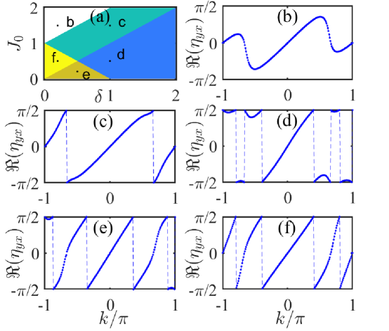
Figure S4: (a) The phase diagram of the 1D chiral-symmetric topological systems. The white, blue, green, dark-yellow and bright-yellow regions respectively share winding number as $w_{\pm}=0,1/2,1,3/2$, and $2$. (b)-(f) $\Re(\eta_{y,x})$ as a function of $k$ in different parameters ($J_{0},\delta$), which are ($1.5,0.2$), ($1.5,1$), ($0.5,1$), ($0.2,0.5$) and ($0.5,0.2$), corresponding to points $b,c,d,e$ and $f$ in (a), respectively. The other parameters are chosen as $J_{1}=1$, $J_{2}=1$ and $h_{z}=0$.

To numerically verify our theory, we consider the systems with $h_{x}=J_{0}+J_{1}\cos(k)+J_{2}\cos(2k)$ and $h_{y}=J_{1}\sin(k)+J_{2}\sin(2k)-i\delta$. In the non-Hermitian case with $\delta\neq 0$, the conventional winding numbers $w_{\pm}$ can appear half integer values in some parameter ranges, different from the integer values in the Hermitian systems. For simplicity, we take $J_{1}=1$, and $J_{0}$, $J_{2}$, $\delta$ are real. The dispersion of this Hamiltonian is

$$\varepsilon_{\pm}(k)=\pm\sqrt{(J_{0}-\delta+e^{-ik}+J_{2}e^{-2ik})(J_{0}+\delta+e^{ik}+J_{2}e^{2ik})}.$$ (S22)

The energy is symmetric about zero energy, which is ensured by the chiral symmetry. Since the energy gap must close at phase transition points, we can determine the phase boundaries by the band-crossing condition $\varepsilon_{\pm}(k)=0$, which yields $J_{0}=\pm\delta+1-J_{2}$ and $J_{0}=\pm\delta-1-J_{2}$ for arbitrary $J_{2}$. Particularly, $J_{0}=J_{2}\pm\delta$ if $|J_{2}|>0.5$. Fixing $J_{1}=1$, $J_{2}=1$ and $h_{z}=0$ and changing both $\delta$ and $J_{0}$, we calculate topological phase diagram distinguished by their winding numbers, see Fig. S4 (a). Here, the white, blue, green, dark-yellow and bright-yellow regions possess conventional winding number $w_{\pm}=0,1/2,1,3/2$ and $2$, respectively. In Figs. S4 (b)-(f), we also give the angle $\Re(\eta_{yx})$ as a function of quasi-momentum $k$ with different parameters ($J_{0},\delta$) marked as b, c, d, e, f in the Figs. S4 (a). The dynamic winding number are $0$, $1$, $1/2$, $3/2$ and $2$, respectively. The numerical results are in well agreement with the theoretical prediction, which prove the validity for our dynamic approach once again.

S3.2 B. Non-chiral symmetric systems

When $h_{z}\neq 0$, the Hamiltonian (S17) breaks the chiral symmetry. Unlike the systems with chiral symmetry, the conventional winding number for each band is not a quantized number, which indicates that $w_{\pm}$ is no longer a topological invariant. However, the sum of the winding numbers for different bands,

$$w_{t}=w_{+}+w_{-}=\frac{1}{\pi}\oint_{S}dk\frac{h_{x}\partial_{k}h_{y}-h_{y}\partial_{k}h_{x}}{h_{x}^{2}+h_{y}^{2}},$$ (S23)

has been demonstrated to be a topological invariant Jiang et al. (2018). The topological invariant $w_{t}$ is independent of $h_{z}$, although its definition is related to the eigenvector of $H(k)$. The parameters $h_{x}$ and $h_{y}$ become very important for the definition of topological invariant. Except for the exceptional point $h_{x}^{2}+h_{y}^{2}=0$, we introduce a complex angle $\phi_{yx}$ satisfying $\tan(\phi_{yx})=h_{y}/h_{x}$. In terms of $\phi_{yx}$, $w_{t}$ can be represented as

$$w_{t}=\frac{1}{\pi}\oint_{S}\partial_{k}\phi_{yx}dk,$$ (S24)

where the integral is also taken along a loop with $k$ from $0$ to $2\pi$. According to Eq. (LABEL:sdynwinding_20190628), we can relate the topological invariant $w_{t}$ to the dynamic winding number

$$w_{t}=w_{+}+w_{-}=2w_{d},$$ (S25)

under a few constraints of initial state: $|c_{+}|^{2}\neq|c_{-}|^{2}$ for Hermitian systems and $|c_{+}|^{2}\neq 0\bigcap|c_{-}|^{2}\neq 0$ for non-Hermitian systems. Fixing $J_{1}=1$, $J_{2}=0$ and $h_{z}=0.5$ in the same model as that in Subsec. LABEL:sChiralSystem, we calculate the topological invariant $w_{t}$ as a function of $\delta$ and $J_{0}$, see Fig. S5 (a). Here, the white, green, and bright-yellow regions possess topological invariant $w_{t}=0,1$ and $2$, respectively. In Figs. S5 (b)-(f), we also give the angle $\Re(\eta_{yx})$ versus the quasi-momentum $k$ with different parameters ($J_{0},\delta$) marked as b, c, d, e, f in the Fig. S5 (a). The dynamic winding number are $0$, $1/2$, $1$, $1/2$ and $0$, respectively. The numerical results are also in well agreement with the theoretical prediction, which demonstrate the validity of our dynamic approach.

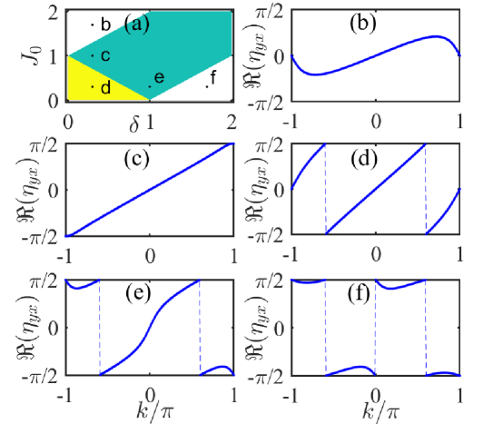
Figure S5: (a) The phase diagram of the 1D non-chiral-symmetric topological systems. The white, green and yellow regions share winding number as $w_{t}=0,1$,and $2$, respectively. (b)-(f) $\Re(\eta_{yx})$ as a function of $k$ in different parameters ($J_{0},\delta$), which are ($1.7,0.3$), ($1,0.3$), ($0.3,0.3$), ($0.3,1$) and ($0.3,1.7$), corresponding to points $b,c,d,e$ and $f$ in (a), respectively. The other parameters are chosen as $J_{1}=1$, $J_{2}=0$ and $h_{z}=0.5$.

S4 S4. Chern number in 2D systems

S4.1 A. Alternate choice of reference axis

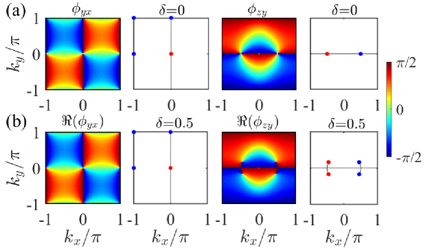
Figure S6: Topologically nontrivial phase with Chern number $C=1$. Hermitian case: (a) Azimuthal angle $\phi_{yx}$ and $\phi_{zy}$ in parameter space ($k_{x},k_{y}$), where blue and red points represent north and south poles of the Bloch spherical surface. Non-Hermitian case: (b) azimuthal angle $\Re(\phi_{yx})$ and $\Re(\phi_{zy})$ in parameter space ($k_{x},k_{y}$). where blue and red points represent north and south EPs of the virtual Bloch spherical surface.

In our main text, we only consider $\theta=\theta_{y}=\arccos(h_{y}/|\vec{h}(\bm{k})|)$ and $\phi=\phi_{xz}=\arctan(h_{x}/h_{z})$. Alternatively, we can also take $\theta=\theta_{z}=\arccos(h_{z}/|\vec{h}(\bm{k})|)$ and $\phi=\phi_{yx}=\arctan(h_{y}/h_{x})$, or $\theta=\theta_{x}=\arccos(h_{x}/|\vec{h}(\bm{k})|)$ and $\phi=\phi_{zy}=\arctan(h_{z}/h_{y})$. These two choices lead to distinct observations, but give the same Chern number. In Fig. S6(a) and (b), based on different choices of reference axis, we give the azimuthal angle $\phi_{yx}$ and $\phi_{zy}$ in Hermitian($\delta=0$) and non-Hermitain($\delta=0.5$) cases, where the other parameters are the same as the Fig. 2(c) of the main text. Around the singularity points, one can also easily obtain the dynamic winding number, and the Chern number $C=1$ in both the Hermitian and non-Hermitian cases, consistent with the ideal Chern number. This is because the different references only differ from a gauge transformation and the Chern number do not depend on the choice of reference.

S4.2 B. Larger Chern number

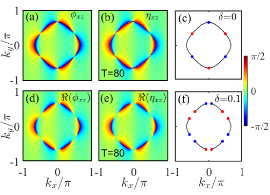
Figure S7: Topologically nontrivial phase with Chern number $C=3$. Hermitian case at top: (a) and (b) correspond to the azimuthal angle $\phi_{xz}$ and $\eta_{xz}$ in parameter space ($k_{x},k_{y}$). (c) Blue and red points represent north and south poles of the Bloch spherical surface. Non-Hermitian case at bottom: (d) and (e) respectively correspond to the azimuthal angle $\Re(\phi_{xz})$ and $\Re(\eta_{xz})$ in parameter space ($k_{x},k_{y}$). (f) Blue and red points represent north and south EPs of the virtual Bloch spherical surface.

The dynamic approach is clearly applicable to topological phases with larger Chern numbers. To show this, we consider another two-band model which supports band structure with larger Chern number, this is,

$$h_{x} = J_{x}\sin(2k_{x});h_{y}=J_{y}\sin(2k_{y});h_{z}=m_{z}-J_{z}\cos(k_{x})-J_{z}\cos(k_{y})-i\delta.$$ (S26)

For the Hermitian case $\delta=0$, the trivial phase is lying in $|m_{z}|>2J_{z}$, while the topological phases are distinguished as: ($i$) $J_{z}<m_{z}<2J_{z}$ with the Chern number $C=-1$; ($ii$) $0<m_{z}<J_{z}$ with $C=3$; ($iii$) $-J_{z}<m_{z}<0$ with $C=-3$; ($iv$) $-2J_{z}<m_{z}<-J_{z}$ with $C=1$. Here we only verify topological phase with Chern number $C=3$, where the other parameters are chosen as $J_{x}=J_{y}=0.2,\ J_{z}=1$ and $m_{z}=0.5$. In Figs. S7(a) and S7(b), we give the azimuthal angle $\phi_{xz}$ and $\eta_{xz}$ in parameter space $(k_{x},k_{y})$, respectively. One can find that more north and south poles appear in Fig. S7(c), compared with Fig. 2 in the main text. From the Eq. (10) in main text, one can also easily obtain the Chern number $C=3$ via dynamic winding number. For the non-Hermitian case, we consider $\delta=0.1$ and the other parameters are the same as those in the Hermitian case. In Figs. S7(d) and S7(e), we also give the azimuthal angle $\Re(\phi_{xz})$ and $\Re(\eta_{xz})$ in parameter space $(k_{x},k_{y})$, respectively. The dynamic winding numbers around EPs become half, while the EPs become double as the Hermitian counterpart, see Fig. S7(f). Eventually, the Chern number keeps the same as that in the Hermitian case.

S5 S5. Experimental consideration

One can immediately apply the dynamical approach for topological Hermitian systems. Cold atom systems is an excellent platform to realize topological band models and detect topological invariants. One and two dimensional spin-orbit couplings have been realized in a highly controllable Raman lattice Qu et al. (2013); Hamner et al. (2014); Sun et al. (2018a, b). Initial states are quite easily prepared by loading the atoms into the lattices. Here, the initial constraint $|c_{\bm{k}+}|^{2}\neq|c_{\bm{k}-}|^{2}$ may be not satisfied for some specific momentum $\bm{k}$, but the occurred probability is so small that the global dynamical azimuthal angle is not affected due to the topological nature. The spin population $N_{\uparrow(\downarrow)}(\bm{k})$ with different momentum can be measured by spin-resolved time-of-flight (TOF) absorption imagingSun et al. (2018b). Thus, one can obtain the spin population difference $\langle\psi_{\bm{k}}(t)|\sigma_{z}|\psi_{\bm{k}}(t)\rangle=(N_{\uparrow}(\bm{k})-N_{\uparrow}(\bm{k}))/(N_{\uparrow}(\bm{k})+N_{\uparrow}(\bm{k}))$. The spin textures $\langle\psi_{\bm{k}}(t)|\sigma_{x(y)}|\psi_{\bm{k}}(t)\rangle$ can be transferred to the spin population difference by applying $\pi/2$ pulse, that is, $\langle\psi_{\bm{k}}(t)|\sigma_{x(y)}|\psi_{\bm{k}}(t)\rangle=\langle\psi_{\bm{k}}(t)|e^{-i\frac{\pi}{2}\frac{\sigma_{y(x)}}{2}}\sigma_{z}e^{i\frac{\pi}{2}\frac{\sigma_{y(x)}}{2}}|\psi_{\bm{k}}(t)\rangle$. Because the cold atom systems have long coherent time, there is no obstacle to extract the dynamic winding number via long time average of the spin textures.

To apply the dynamical approach in topological non-Hermitian systems, we should first consider how to realize the topological non-Hermitian models in experiments. Since two-level non-Hermitian models have been widely realized in optical systems, such as two coupled optical cavities Chang et al. (2014); Peng et al. (2014), optical waveguides Gordon and Kogelnik (2000); Rüter et al. (2010); Zeuner et al. (2015), optomechanical cavityAspelmeyer et al. (2014); Xu et al. (2016); Verhagen and Alù (2017) etc. We mainly discuss how to extract dynamic winding number with two optical waveguides with tunable parameters. A two-level non-Hermitian system can be realized by introducing gain and loss in the two waveguides. The coupling strength can be tuned by the waveguide separation. We regard the two different waveguides as two spin components. The initial states can be prepared by randomly split the light injecting into the two waveguides. One can obtain $\langle\psi(l)|\sigma_{z}|\psi(l)\rangle$ by measuring the intensity difference between two waveguides at propagating distance $l$. Here, the distance $l$ plays the role of time. Actually, the final states will collapse into one of the eigenstate in the long distance. Thus, the output intensity difference of the waveguides is sufficient and long distance average of the intensity difference is not necessary. One can also obtain $\langle\psi(l)|\sigma_{x(y)}|\psi(l)\rangle$ by insetting a beam splitter before intensity measurement. By designing the waveguide separation and gain and loss rates, one can simulate the two-band model. Repeating the above operations, one can finally construct the dynamic winding number.

References

- Yin et al. (2018) C. Yin, H. Jiang, L. Li, R. Lü, and S. Chen, “Geometrical meaning of winding number and its characterization of topological phases in one-dimensional chiral non-Hermitian systems,” Phys. Rev. A 97, 052115 (2018).
- Jiang et al. (2018) H. Jiang, C. Yang, and S. Chen, “Topological invariants and phase diagrams for one-dimensional two-band non-Hermitian systems without chiral symmetry,” Phys. Rev. A 98, 052116 (2018).
- Qu et al. (2013) C. Qu, C. Hamner, M. Gong, C. Zhang, and P. Engels, “Observation of Zitterbewegung in a spin-orbit-coupled Bose-Einstein condensate,” Phys. Rev. A 88, 021604 (2013).
- Hamner et al. (2014) C. Hamner, C. Qu, Y. Zhang, J. Chang, M. Gong, C. Zhang, and P. Engels, “Dicke-type phase transition in a spin-orbit-coupled Bose–Einstein condensate,” Nat. commun. 5, 4023 (2014).
- Sun et al. (2018a) W. Sun, B. Z. Wang, X. T. Xu, C. R. Yi, L. Zhang, Z. Wu, Y. Deng, X. J. Liu, S. Chen, and J. W. Pan, “Highly controllable and robust 2D spin-orbit coupling for quantum gases,” Phys. Rev. Lett. 121, 150401 (2018a).
- Sun et al. (2018b) W. Sun, C. R. Yi, B. Z. Wang, W. W. Zhang, B. C. Sanders, X. T. Xu, Z. Y. Wang, J. Schmiedmayer, Y. Deng, X. J. Liu, et al., “Uncover topology by quantum quench dynamics,” Phys. Rev. Lett. 121, 250403 (2018b).
- Chang et al. (2014) L. Chang, X. Jiang, S. Hua, C. Yang, J. Wen, L. Jiang, G. Li, G. Wang, and M. Xiao, “Parity–time symmetry and variable optical isolation in active–passive-coupled microresonators,” Nat. photon. 8, 524 (2014).
- Peng et al. (2014) B. Peng, Ş. K. Özdemir, F. Lei, F. Monifi, M. Gianfreda, G. L. Long, S. Fan, F. Nori, C. M. Bender, and L. Yang, “Parity–time-symmetric whispering-gallery microcavities,” Nat. Phys. 10, 394 (2014).
- Gordon and Kogelnik (2000) J. P. Gordon and H. Kogelnik, “Pmd fundamentals: Polarization mode dispersion in optical fibers,” Proc. Natl. Acad. Sci. 97, 4541–4550 (2000).
- Rüter et al. (2010) C. E. Rüter, K. G. Makris, R. El-Ganainy, D. N. Christodoulides, M. Segev, and D. Kip, “Observation of parity–time symmetry in optics,” Nat. Phys. 6, 192 (2010).
- Zeuner et al. (2015) J. M. Zeuner, M. C. Rechtsman, Y. Plotnik, Y. Lumer, S. Nolte, M. S. Rudner, M. Segev, and A. Szameit, “Observation of a topological transition in the bulk of a non-Hermitian system,” Phys. Rev. Lett. 115, 040402 (2015).
- Aspelmeyer et al. (2014) M. Aspelmeyer, T. J. Kippenberg, and F. Marquardt, “Cavity optomechanics,” Rev. Mod. Phys. 86, 1391 (2014).
- Xu et al. (2016) H. Xu, D. Mason, L. Jiang, and J. G. E. Harris, “Topological energy transfer in an optomechanical system with exceptional points,” Nature 537, 80 (2016).
- Verhagen and Alù (2017) E. Verhagen and A. Alù, “Optomechanical nonreciprocity,” Nat. Phys. 13, 922 (2017).