Low-energy bound states, resonances, and scattering of light ions

Abstract

We describe bound states, resonances and elastic scattering of light ions using a $\delta$-shell potential. Focusing on low-energy data such as energies of bound states and resonances, charge radii, asymptotic normalization coefficients, effective-range parameters, and phase shifts, we adjust the two parameters of the potential to some of these observables and make predictions for the nuclear systems $d+\alpha$, $\mbox{${}^{3}$He}+\alpha$, $\mbox{${}^{3}$He}+\alpha$, $\alpha+\alpha$, and $p+\mbox{${}^{16}$O}$. We identify relevant momentum scales for Coulomb halo nuclei and propose how to apply systematic corrections to the potentials. This allows us to quantify statistical and systematic uncertainties. We present a constructive criticism of Coulomb halo effective field theory and compute the unknown charge radius of ¹⁷F.

I Introduction

Low-energy reactions between light ions fuel stars and are relevant to stellar nucleosynthesis Adelberger et al. (2011). Because of the Coulomb barrier, fusion cross sections decrease exponentially with decreasing kinetic energy of the reactants, and this makes it difficult to measure them in laboratories. For the extrapolation of data to low energies, and a quantitative understanding of the reactions one thus has to turn to theoretical calculations.

Theoretical approaches can roughly be divided into two kinds, taking either the ions as degrees of freedom or starting from individual nucleons. The former approach includes a variety of models Buck et al. (1975); Kulik and Mur (2003); Typel and Baur (2005); Grassi et al. (2017), effective range expansions Hamilton et al. (1973); Mur and Popov (1985); Mur et al. (1993); Sparenberg et al. (2010); Yarmukhamedov and Baye (2011); Ramírez Suárez and Sparenberg (2017); Blokhintsev et al. (2018), and effective field theories (EFTs) Higa et al. (2008); Ryberg et al. (2014a); Zhang et al. (2014); Higa et al. (2018); Capel et al. (2018); Zhang et al. (2018); the microscopic approach ranges from simpler models Neff (2011) to ab initio computations Nollett et al. (2001); Quaglioni and Navrátil (2008); Hupin et al. (2015); Dohet-Eraly et al. (2016). Unfortunately, there are still significant uncertainties Adelberger et al. (2011), and data tables for relevant quantities such as asymptotic normalization coefficients (ANCs) or astrophysical $S$ factors may Dubovichenko and Dzhazairov-Kakhramanov (2017) or may not Descouvemont et al. (2004); Huang et al. (2010) contain theoretical uncertainties.

There are various tools available for computing theoretical uncertainties Dobaczewski et al. (2014); Furnstahl et al. (2015). Systematic errors are accessible within EFTs (because of a power counting) Schindler and Phillips (2009); Furnstahl et al. (2015, 2015); Coello Pérez and Papenbrock (2015); Carlsson et al. (2016) but much harder to quantify for models. Nevertheless, all models are constrained by data with errors, and the propagation of the latter to computed observables, or the employment of a set of models provides us with means to uncertainty estimates Dobaczewski et al. (2014).

In this work, we revisit low-energy bound states, resonances, and scattering within simple two-parameter models, using ions as the relevant degrees of freedom. In an attempt to estimate uncertainties, we quantify the sensitivity of the computed results to the input data. We also propose systematic improvements of the simple models. This allows us to estimate model uncertainties. As we will see, this approach yields accurate results when compared to data. One of the key results is the prediction for the unknown charge radius of ¹⁷F. We contrast our approach to Coulomb halo EFT (which is not accurate at leading order for ⁸Be Higa et al. (2008) and ¹⁷F Ryberg et al. (2014a)) and present a constructive criticism based on a finite range and a modified derivative expansion.

This paper is organized as follows. In Section II we present arguments in support of finite-range interactions, review key formulas for the $\delta$-shell potential, and discuss systematic improvements. Section III shows the results for a number of interesting light-ion systems. We conclude with a summary in Sect. IV. Several details are relegated to the Appendix V.

II Theoretical background

II.1 Energy scales and estimates for observables

While effective range expansions Mur and Popov (1985); Mur et al. (1993); Sparenberg et al. (2010) established relations between low-energy observables, we still lack simple expressions that give estimates for such observables when only basic properties such as energies and radii of the involved ions are available. In applications of EFTs to low-energy ion scattering one makes assumptions about the relevant momentum scales to propose a power counting Higa et al. (2008); Ryberg et al. (2014a); Zhang et al. (2014); Capel et al. (2018). This makes it important to understand the relevant scales. As it turns out, the presence of Coulomb interactions modifies expectations from neutron-halo EFT or pion-less EFT significantly. To see this, we explore how a finite-range potential differs from a zero-range potential.

The range of the strong nuclear force is close to the sum of the (charge) radii $D$ of two interacting particles. This is true for both, the nucleon-nucleon interaction and for the strong force between ions considered in this work. It is in this sense that the nuclear interaction is short ranged. This implies that the two-body wave function essentially acquires its “free” asymptotic form for inter-particle distances $r\gtrsim D$.

The relevant asymptotic properties of a low-energy bound-state wave function are its binding momentum and ANC. In the absence of the Coulomb interaction, the $s$-wave ANC $C_{0}$ is related to the bound-state momentum $\gamma$ for weakly bound states via $C_{0}^{2}\approx 2\gamma$. Similarly , the $s$-wave scattering length $a_{0}$ fulfills $a_{0}\approx 1/\gamma$. This allows one – at leading order – to work with zero-range potentials. We note that the effective range scales as $r_{0}\sim{\cal O}(D)$. Finite-range effects of the potential enter at next-to-leading order. Pion-less EFT and neutron-halo EFT are based on these insights Bedaque and van Kolck (2002); Bertulani et al. (2002); Hammer et al. (2017).

Let us now contrast this to the case when the Coulomb potential

$$V_{C}(r)={\hbar^{2}k_{c}\over mr}$$ (1)

is added. Here, $m$ is the reduced mass and $k_{c}$ is the Coulomb momentum (or inverse Bohr radius)

$$k_{c}\equiv{Z_{1}Z_{2}\alpha m\over\hbar}.$$ (2)

It is given in terms of the fine structure constant $\alpha\approx 1/137$ and the charge numbers $Z_{1}$ and $Z_{2}$ of the two ions. As we will see, this new momentum scale significantly modifies the discussion of low-energy observables.

We consider a weakly bound state with energy $-\hbar^{2}\gamma^{2}/(2m)$ and bound-state momentum $\gamma$, and assume $\gamma\ll k_{c}$; for resonances we consider a low-energy resonance with energy $\hbar^{2}\kappa^{2}/(2m)$ and momentum $\kappa$, and also assume $\kappa\ll k_{c}$. In what follows, we will simply refer to these momenta as $k$, setting $k=i\gamma$ for bound states and $k=\kappa$ for resonances. The Sommerfeld parameter is

$$\eta\equiv{k_{c}\over k}.$$ (3)

For radial distances $r$ approximately exceeding the sum $D$ of the charge radii of the two ions, the strong interaction potential vanishes, and the Hamiltonian consists of the kinetic energy and the Coulomb potential. Thus, for $r\gtrsim D$, the wave functions are combinations of Coulomb wave functions. For small momenta $|k|\ll k_{c}$, the Coulomb wave functions can be expanded in a series of modified Bessel functions, where coefficients fall off as inverse powers of $\eta$, while the modified Bessel functions have arguments $2\sqrt{2k_{c}r}$ (see the Appendix for details). Thus, low-energy observables (such as ANCs, radii, scattering lengths, and effective ranges) become series of functions of $2\sqrt{2k_{c}D}$, with coefficients that fall off as inverse powers of $|\eta|$. Let us contrast the case $D\to 0$ of zero-range interactions and the case $2\sqrt{2k_{c}D}\gg 1$. Estimates for several low-energy $s$-wave observables are given in Table 1, based on calculations with a $\delta$-shell potential Mur et al. (1993) (with details of the calculation presented in the Appendix).

Observable	$2\sqrt{2k_{c}D}\gg 1$	$D\to 0$
$a_{0}$	$-(\pi\kappa^{2}D)^{-1}e^{4\sqrt{2k_{c}D}}$	$-{6k_{c}\over\kappa^{2}}$
$r_{0}$	$(3k_{c})^{-1}$	${\cal O}(D)$
$C_{0}$	$(\pi D)^{-1/2}\Gamma(1+k_{c}/\gamma)e^{2\sqrt{2k_{c}D}}$	$\sqrt{6k_{c}}\Gamma(1+k_{c}/\gamma)$
${\Gamma\over E}$	$4{k_{c}\over\kappa^{2}D}e^{4\sqrt{2k_{c}D}}e^{-2\pi{k_{c}\over\kappa}}$	$24\pi{k_{c}^{2}\over\kappa^{2}}e^{-2\pi{k_{c}\over\kappa}}$
$\langle r^{2}\rangle$	$D^{2}$	${\cal O}(k_{c}^{-2})$

Table 1: Simple estimates for low-energy observables of a two-ion system with a bound-state momentum $\gamma$ or a resonance momentum $\kappa$, in presence of a Coulomb potential with the Coulomb momentum $k_{c}$, and a $\delta$-shell potential with the range $D$, in the limit $\kappa,\gamma\ll k_{c}$. Here $a_{0}$, $r_{0}$, $C_{0}$, and $\Gamma/E$ are the $s$-wave scattering length, effective range, and ANC, respectively. The resonance energy is $E=\hbar^{2}\kappa^{2}/(2m)$, and the corresponding width is denoted as $\Gamma$, not to be confused with the Gamma function $\Gamma(1+k_{c}/\gamma)$. The inter-ion distance is $\langle r^{2}\rangle$.

We see that the scattering length $a_{0}$, the squared ANC $C_{0}^{2}$, and the resonance width are exponentially enhanced by a factor $e^{4\sqrt{2k_{c}D}}$ when $k_{c}D\gg 1$ compared to the case $D\to 0$. We also see that the inter-ion distance squared $\langle r^{2}\rangle$ is not large, though we considered the limit of vanishing bound-state momentum. However, this distance becomes very small in the zero-range limit. It is clear that a zero-range potential is not compatible with nuclei: As ions have finite charge radii they must be separated by a distance that is similar to the sum of their charge radii in order to retain their identities. An EFT that employs a contact at leading order fails short of this requirement. These arguments confirm the need to include finite-range potentials or a finite effective range at leading order Higa et al. (2008); Papenbrock ; Schmickler et al. (2019).

On the first view, the quantities displayed in the second column of Table 1 appear to be model dependent for $2\sqrt{2k_{c}D}\gg 1$ (as they depend on the parameter $D$). However, in the considered limit, the inter-ion distance fulfills $\langle r^{2}\rangle=D^{2}$, and this links observable quantities to each other.

The inter-ion distance is related to the charge radius. Let the ions (labeled by $i=1,2$) have masses $m_{i}$ and charge radii squared $\langle r_{i}^{2}\rangle$. Then, the charge radius squared of the bound state is Buck and Pilt (1977)

$$\langle R_{c}^{2}\rangle={Z_{1}\langle r_{1}^{2}\rangle+Z_{2}\langle r_{2}^{2}\rangle\over Z_{1}+Z_{2}}+\frac{(Z_{1}m_{2}^{2}+Z_{2}m_{1}^{2})\langle r^{2}\rangle}{(Z_{1}+Z_{2})(m_{1}+m_{2})^{2}}.$$ (4)

Here, the first term account for the finite charge radii of the ions, and the second term is the contribution of the ions (taken as point charges) in the center-of-mass system. The derivation of Eq. (4) is elementary and this expression is well known Buck et al. (1975); Buck and Pilt (1977); for a recent EFT discussion of contributions to charge radii in halo nuclei we refer the reader to Ref. Ryberg et al. (2019). We note that the consistency of any two-ion model (or EFT) requires that the distance between the two ions is larger than the sum of their individual charge radii. As we will see below, our results are largely consistent with the assumption of separated ions.

We also note that cluster systems consisting of an even-even and an odd-mass nucleus have magnetic moments (in units of nuclear magnetons)

$$\mu=\mu_{\rm odd}+{Z\over A}l.$$ (5)

Here, $\mu_{\rm odd}$ is the magnetic moment of the odd-mass constituent, $l$ is the orbital angular momentum, and $Z$ and $A$ are the charge and mass number, respectively, of the compound system. Here we assumed that the magnetic moment due to the spin $S$ of the odd-mass ion and the magnetic moment due to the orbital angular momentum $l$ add up. This is the case for states with total spin $j=l+S$.

We note that (for $2\sqrt{2k_{c}D}\gg 1$) the effective range in Table 1 does not depend on $D$, and that it decreases with increasing Coulomb momentum. Its value, $r_{0}=1/(3k_{c})$, is that of a Coulomb system with a zero-energy bound state (see Appendix for details), and $1/(3k_{c})$ is also at the causality limit imposed by the Wigner bound Mur et al. (1993); König et al. (2013). We can define the nontrivial regime of strong Coulomb interactions by the model-independent relation $3k_{c}r_{0}\approx 1$. For the $\delta$-shell potential, is interesting to compute corrections that are due to a finite value of $2k_{c}D$. This yields Mur et al. (1993) (see the Appendix for details)

$$r_{0}-{1\over 3k_{c}}=-\pi De^{-4\sqrt{2k_{c}D}}.$$ (6)

This equation expresses model-dependent quantities on its right-hand side in terms of observables. Combining it with the expression for the scattering length in Table 1 yields the model-independent relation

$$\kappa^{-2}=a_{0}\left(r_{0}-{1\over 3k_{c}}\right).$$ (7)

This formula was derived (for bound states) by Sparenberg et al. (2010) and very recently rederived by Schmickler et al. (2019).

Other notable relations that can be obtained from Table 1 are

$$a_{0} \approx -(4\pi k_{c})^{-1}{\Gamma\over E}e^{2\pi{k_{c}\over\kappa}},$$ (8)

relating the scattering length to resonance properties, and

$$C_{0}^{2} \approx \gamma^{2}a_{0}\left[\Gamma(1+k_{c}/\gamma)\right]^{2},$$ (9)

relating the ANC to the bound-state energy and the scattering length (after replacing $\kappa$ by $\gamma$). This last expression agrees with the result in Refs. Sparenberg et al. (2010); König et al. (2013). It seems to us that Eq. (8) was not yet known. These model-independent expressions are valuable. They relate quantities that are often unknown or hard to measure (such as the ANC or the effective range parameters) to others that are better known (such as energies or widths).

We believe the expressions in Table 1 are also useful, because they allow us to estimate these hard-to-measure quantities. Table 2 lists relevant parameters for two-ion systems of interest. Of the considered systems, only the last two approximately fulfill both $|\eta|\gg 1$ and $2\sqrt{2k_{c}D}\gg 1$. Thus, for theses systems, finite-range models will yield significantly different values than zero-range models. Applying the simple expressions of Table 1 and the estimates for $D$ from Table 2 to $\alpha-\alpha$ scattering yields a very large scattering length of about $a_{0}\approx-2482$ fm, an effective range $r_{0}\approx 1.2$ fm, and a resonance width of $\Gamma\approx 7.5$ eV. These values are reasonably close to actual values. For the weakly bound $J^{\pi}=1/2^{+}$ state of the $p+\mbox{${}^{16}$O}$ system, we note that the simple estimate from Table 1 yields an ANC of about $C_{0}\approx 80$ fm^-1/2, close to the empirical estimates Gagliardi et al. (1999); Artemov et al. (2009); Huang et al. (2010); Yarmukhamedov and Baye (2011). Thus, we gained an understanding of the scales involved in Coulomb halo nuclei.

System	$J^{\pi}$	$\gamma$ or $\kappa$ (fm-1)	$k_{c}$ (fm-1)	$D$ (fm)	$2\sqrt{2k_{c}D}$
$d+\alpha$	$1^{+}$	0.31	0.09	3.82	1.68
$\mbox{${}^{3}$H}+\alpha$	$3/2^{-}$	0.45	0.12	3.43	1.80
$\mbox{${}^{3}$He}+\alpha$	$3/2^{-}$	0.36	0.24	3.64	2.63
$p+\mbox{${}^{7}$Be}$	$1/2^{-}$	0.08	0.12	3.52	1.85
$\alpha+\alpha$	$0^{+}$	0.09	0.28	3.35	2.72
$p+\mbox{${}^{16}$O}$	$1/2^{+}$	0.07	0.26	3.58	2.73

Table 2: Bound-state momentum $\gamma$ (or momentum $\kappa$ of the resonant state), Coulomb momentum $k_{c}$, and sum of charge radii $D$ for two-ion systems in the state with spin/parity $J^{\pi}$. The dimensionless quantity $2\sqrt{2k_{c}D}$ is also shown.

Table 2 shows that $2\sqrt{2k_{c}D}\gtrsim 1$ for essentially all Coulomb halo nuclei of interest. As a consequence, $r_{0}-1/(3k_{c})$ is very small for $s$ waves, and this makes scattering lengths, resonance widths, and ANCs large. We note that these are natural properties of Coulomb-halo nuclei. In contrast, the smallness of $r_{0}-1/(3k_{c})$ is viewed as a fine tuning in Coulomb halo EFT Higa et al. (2008); Ryberg et al. (2014a); Higa et al. (2018).

In what follows, we will exploit a separation of scales between the low momentum scale we are interested in and a higher-lying breakdown scale. The breakdown momentum $\Lambda_{b}$ is set by the smaller of an empirical and a theoretical breakdown scale. The empirical breakdown scale is set by the energy of excited states of the two clusters or of the resulting nucleus; however, only states with relevant quantum numbers count. In ⁸Be, for instance, the ground state has spin/parity $J^{\pi}=0^{+}$, and the empirical breakdown scale is set by first excited $0^{+}$ state at about 20 MeV (and not by the energy of the lowest $2^{+}$ state at 3 MeV). There is also a theoretical breakdown scale. The strong interaction potential has a range that is of the size of the sum $D$ of the charge radii of the clusters involved. Thus, at momenta $\pi/D$, the details of our model are fully resolved. As we cannot expect that the $\delta$-shell model would be accurate at such a high momentum, it sets the theoretical breakdown scale. In other words: this is the momentum where different models with a physical range $D$ will differ significantly from each other.

The phenomena we seek to describe are simple because of the empirical scale separation. Scattering phase shifts at low energies are typically either close to zero or close to $\pi$. Only in presence of a narrow resonance do phase shifts vary rapidly in a small energy region of the size of the resonance width. Thus, away from the resonance energy, the asymptotic wave function consists mostly of the regular Coulomb wave function, which is exponentially small under the Coulomb barrier. This implies that the wave function cannot resolve any details of a finite-range potential as long as the classical turning point is larger than the range $D$ of our potential. The corresponding “model” momentum $\Lambda_{m}$ fulfills

$$\Lambda_{m}\equiv\sqrt{2k_{c}/D}.$$ (10)

Thus, for momenta below $\Lambda_{m}$, it will be hard to distinguish between different finite-range models that have been adjusted to low-energy data. In this sense, one deals with universal and model-independent phenomena. For momenta $k$ with $\Lambda_{m}\lesssim k\lesssim\pi/D$ differences between models start to show up and eventually become fully resolved. Some models might accurately describe data even for momenta beyond $\Lambda_{m}$; we would view such models as fortuitous but useful picks. The systematic improvements presented in the previous Subsection can be used to estimate what a different model would yield; we refer to resulting uncertainties as “systematic uncertainties” in what follows. In EFT parlance, the momentum regime below $\Lambda_{m}$ would be that where “leading-order” results are expected to be accurate and precise. Higher-order corrections should become visible beyond that scale.

In this work, we employ simple finite-range models for the nuclear potential that essentially exhibit two parameters (a range and a strength). Most calculations will be done with the $\delta$-shell potential, but for ⁸Be we also employ a simple square well or the Breit model Breit and Bouricius (1948), a hard-core potential plus a boundary condition. As we will see, at sufficiently low energies, and when adjusted to low-energy data, such simple models will describe data accurately and precisely. We will also propose how to make systematic improvements to these models.

II.2 $\delta$-shell potential

The $\delta$-shell potential plus the Coulomb interaction is well understood and can be solved analytically Kok et al. (1982); Mur and Popov (1985); Mur et al. (1993). In this Subsection, we briefly summarize some of the relevant results. The Hamiltonian is

$$H=H_{0}+V.$$ (11)

The strong interaction potential is $V$, and the “free” Hamiltonian $H_{0}$ consists of the kinetic energy and the Coulomb interaction

$$H_{0}=-{\hbar^{2}\over 2m}\Delta+V_{C}(r).$$ (12)

Here, $m$ denotes the reduced mass of the two-ion system and $V_{C}$ is the Coulomb potential (1). The $\delta$-shell potential is parameterized as

$$V(r)={\hbar^{2}\lambda_{0}\over m}\delta(r-R).$$ (13)

Here, $\lambda_{0}$ and $R$ denote the strength and the physical range of the potential, respectively. We work in the center-of-mass system and employ spherical coordinates. The radial wave function $\psi_{l}(r)=u_{l}(r)/r$ must be continuous at $r=R$, and its derivative $u_{l}^{\prime}\equiv{du_{l}\over dr}$ fulfills

$$u_{l}^{\prime}(R^{+})-u_{l}^{\prime}(R^{-})=\lambda_{0}u_{l}(R).$$ (14)

The radii $R^{+}$ and $R^{-}$ are infinitesimal larger and smaller than $R$, respectively.

II.2.1 Bound states

For bound states with energy $E=-{\hbar^{2}\gamma^{2}\over 2m}$ we make the ansatz

$$u_{l}(r)=\left\{\begin{array}[]{ll}N\frac{H_{l}^{+}\left({k_{c}\over i\gamma},i\gamma R\right)}{F_{l}\left({k_{c}\over i\gamma},i\gamma R\right)}F_{l}\left({k_{c}\over i\gamma},i\gamma r\right),&r<R\\ NH_{l}^{+}\left({k_{c}\over i\gamma},i\gamma r\right),&r>R.\end{array}\right.$$ (17)

Here, we employed the Coulomb wave functions $F_{l}$ and $H_{l}^{+}$. As we employ the Coulomb wave functions at imaginary arguments, some care must be taken in their numerical implementation; we followed Gaspard and Sparenberg (2018) and present details in the Appendix. In Eq. (17), the constant $N$ ensures the proper normalization

$$\int\limits_{0}^{\infty}dr\left|u_{l}(r)\right|^{2}=1$$ (18)

of the wave function. Because of the particular ansatz of the wave function for $r>R$, the ANC is

$$C_{l}=N\frac{W_{-k_{c}/\gamma,l+1/2}(2\gamma R)}{H_{l}^{+}\left({k_{c}\over i\gamma},i\gamma R\right)}.$$ (19)

The matching condition (14) yields

$${\gamma\over\lambda_{0}}=iF_{l}\left({k_{c}\over i\gamma},i\gamma R\right)H_{l}^{+}\left({k_{c}\over i\gamma},i\gamma R\right).$$ (20)

The inter-ion distance squared

$$\langle r^{2}\rangle=\int\limits_{0}^{\infty}drr^{2}\left|u_{l}(r)\right|^{2}$$ (21)

enters the computation of the charge radius (4).

II.2.2 Scattering

For positive energies $E={\hbar^{2}k^{2}\over 2m}$ we make the ansatz

$$u_{l}(r)=\left\{\begin{array}[]{ll}BF_{l}\left({k_{c}\over k},kr\right),&r<R\\ F_{l}\left({k_{c}\over k},kr\right)\cos\delta+G_{l}\left({k_{c}\over k},kr\right)\sin\delta,&r>R.\end{array}\right.$$ (24)

Here, $G_{l}$ is the irregular Coulomb wave function, $\delta$ denotes the phase shift, and we employed the shorthand

$$B\equiv\frac{F_{l}\left({k_{c}\over k},kR\right)\cos\delta+G_{l}\left({k_{c}\over k},kR\right)\sin\delta}{F_{l}\left({k_{c}\over k},kR\right)}.$$ (25)

The matching condition (14) yields

$${k\over\lambda_{0}}=-F^{2}_{l}\left({k_{c}\over k},kR\right)\cot\delta-F_{l}\left({k_{c}\over k},kR\right)G_{l}\left({k_{c}\over k},kR\right)$$ (26)

Given the phase shifts, one can use this equation to adjust $\lambda_{0}$. Alternatively, for fixed parameters $(\lambda_{0},R)$ this equation can be solved for the phase shifts. This yields

$$\cot\delta=-\frac{{k\over\lambda_{0}}+F_{l}\left({k_{c}\over k},kR\right)G_{l}\left({k_{c}\over k},kR\right)}{F^{2}_{l}\left({k_{c}\over k},kR\right)}.$$ (27)

The $\delta$-shell potential can at most exhibit one bound state. It is interesting to identify the critical strength $\lambda_{*}$ at which the bound state enters. To do so, we start from Eq. (26), and consider a resonance by setting $\delta=\pi/2$. In order to take the limit $k\to 0$, we employ asymptotic approximations of the Coulomb wave functions (see Appendix for details). This yields

$$\lambda_{*}^{-1}=-2RI_{1}\left(2\sqrt{2k_{c}R}\right)K_{1}\left(2\sqrt{2k_{c}R}\right).$$ (28)

Here, $I_{1}$ and $K_{1}$ are modified Bessel functions.

The effective range-expansion for the $\delta$-shell potential is Kok et al. (1982); Mur and Popov (1985)

$$a_{l}^{-1} = \frac{2k_{c}^{2l+1}}{\left(l!I_{2l+1}\right)^{2}}\left({1\over\lambda_{0}R}+2I_{2l+1}K_{2l+1}\right)$$

$$r_{l} = -\frac{2k_{c}^{2l-1}}{3\left(l!I_{2l+1}\right)^{2}}\bigg{[}2{k_{c}\over\lambda_{0}}{lI_{2l+3}+\sqrt{2k_{c}R}I_{2l+2}\over I_{2l+1}}$$ (29)

$$+2l(l+1)(l+2)I_{2l+1}K_{2l+1}$$

$$-{1\over 2}\left(I_{2l+1}\right)^{2}-l(l+1)-k_{c}R\bigg{]}.$$

Here, we used the shorthands

$$I_{l}\equiv I_{l}\left(2\sqrt{2k_{c}R}\right)$$ (30)

for the modified Bessel functions.

II.2.3 Resonances

As $\lambda_{0}$ is decreased from $0$ at fixed $R$, the potential becomes increasingly more attractive. Just before the critical strength (28) is reached, the phase shift exhibits a quick rise through $\pi/2$ at a low momentum $\kappa$. This is reminiscent of a resonance, and we can indeed model this physical phenomenon. To do so, we set $\delta=\pi/2$ in Eq. (26) and find

$${\kappa\over\lambda_{0}}=-F_{l}\left({k_{c}\over\kappa},\kappa R\right)G_{l}\left({k_{c}\over\kappa},\kappa R\right).$$ (31)

This relates the parameters of our potential to the resonance momentum $\kappa$. The resonance energy is $E=\hbar^{2}\kappa^{2}/(2\mu)$. To compute the resonance width $\Gamma$, we use the relation Wigner (1955)

$${d\delta\over dE}={2\over\Gamma}.$$ (32)

We denote the momentum derivative of a function $f$ as ${df\over dk}\equiv\dot{f}$, take the derivative with respect to momentum of Eq. (26), and set $\delta=\pi/2$. This yields

$$\lambda_{0}^{-1}=\left(F_{l}\right)^{2}\dot{\delta}-\dot{F}_{l}G_{l}-F_{l}\dot{G}_{l}.$$ (33)

Here and in what follows we suppress the arguments $(k_{c}/\kappa,\kappa R)$ of the Coulomb wave functions. Combining Eqs. (31) and (33), and using $\dot{\delta}=4E/(\kappa\Gamma)$ yields an expression for the width that depends on $R$ alone

$${E\over\Gamma}=\frac{\kappa\left(\dot{F}_{l}G_{l}+F_{l}\dot{G}_{l}\right)-F_{l}G_{l}}{4(F_{l})^{2}}.$$ (34)

Given the width and the resonance energy, one can solve Eq. (34) for the parameter $R$; substitution of the result into Eq. (31) then yields the parameter $\lambda_{0}$.

It is now interesting to combine the result (31) with Eq. (26) to compute the phase shift. We find

$$\cot\delta=\frac{{k\over\kappa}F_{l}\left({k_{c}\over\kappa},\kappa R\right)G_{l}\left({k_{c}\over\kappa},\kappa R\right)-F_{l}\left({k_{c}\over k},kR\right)G_{l}\left({k_{c}\over k},kR\right)}{F_{l}^{2}\left({k_{c}\over k},kR\right)}.$$

II.3 Systematic improvements

Let us discuss systematic improvements. Consider the operator

$$W_{n}\equiv{1\over 2}\left(H_{0}\right)^{n}\delta(r-R^{+})+{1\over 2}\delta(r-R^{+})\left(H_{0}\right)^{n}.$$ (36)

Here, $R^{+}$ denotes a point that is larger than $R$ by an arbitrarily small amount, and $n$ is a non-negative integer . Consider the Hamiltonian ($n\geq 1$)

$$\tilde{H}_{n}=H_{0}+V+g_{n}W_{n},$$ (37)

where $g_{n}$ denotes a low-energy constant. We write down the Schrödinger equation for the Hamiltonian $\tilde{H}_{n}$ acting on the eigenfunction of $H_{0}$ with eigenvalue $E$ and integrate over the neighborhood of the singularities at $r=R$. This yields

$$0 = \int\limits_{R^{-}}^{R^{+}}dr\tilde{H}_{n}u_{l}(r)$$

$$= -{\hbar^{2}\over 2m}\left[u^{\prime}_{l}(R^{+})-u^{\prime}_{l}(R^{-})-\lambda_{0}u_{l}(R)\right]+g_{n}E^{n}u_{l}(R^{+})$$

Comparison with Eq. (14) shows that the matching condition becomes

$$u^{\prime}_{l}(R^{+})-u^{\prime}_{l}(R^{-})=\tilde{\lambda}u_{l}(R),$$ (39)

where we introduced the energy-dependent coupling constant

$$\tilde{\lambda} \equiv \lambda_{0}+{2m\over\hbar^{2}}g_{n}E^{n}.$$ (40)

One might prefer to convert energy dependence into a momentum dependence. We employ the shorthand

$$g_{n}=\left({2m\over\hbar^{2}}\right)^{n-1}\tilde{g}_{n},$$ (41)

and $E=\hbar^{2}k^{2}/(2m)$, noting that $k$ can be real (for positive energies) or purely imaginary $k=i\gamma$ for bound states. Then, the momentum-dependent coupling constant is

$$\tilde{\lambda}(k)=\lambda_{0}+\tilde{g}_{n}k^{2n}.$$ (42)

We remind ourselves that this is only correct if the Hamiltonian acts on eigenstates of $H_{0}$. Let us discuss the power counting. The breakdown momentum is $\Lambda_{b}$. By definition, the leading-order Hamiltonian (11) and the perturbation (36) have the same energy $\hbar^{2}\Lambda_{b}^{2}/(2m)$ at the breakdown scale. Equating the respective energies yields the scaling

$$\tilde{g}_{n}\sim\frac{R}{\Lambda_{b}^{2(n-1)}}.$$ (43)

Thus, for “natural” coefficients of that size, the momentum-dependent coupling constant (42) is a small correction at low momenta, and contributions systematically decrease with increasing $n$. We propose that $W_{2}$ is the next-to-leading-order correction to the leading-order Hamiltonian $H$. The rationale is as follows: The two parameters of our theory allow us to fit, for instance, the scattering length and the effective range. Then, a quartic correction at next-to-leading order should affect the shape parameters in the effective range expansion.

We note that the same result could have been obtained from perturbation theory. We also note that the same systematic corrections apply to the Breit model or the square-well potential. The reason is that also for these models the eigenstates of $H=H_{0}+V$ are wave functions of the “free” Hamiltonian $H_{0}$ for $r>R$. Thus, the expectation value of $g_{n}W_{n}$ in a state with energy $E=\hbar^{2}k^{2}/(2m)$ is $(k^{2}/\Lambda_{b}^{2})^{n-1}EC_{l}^{2}R$. The power counting is clearly exhibited, and a systematically improvable Hamiltonian is (terms are ordered in terms of decreasing importance)

$$H = H_{0}+{\hbar^{2}\lambda_{0}\over m}W_{0}+g_{2}W_{2}+g_{3}W_{3}+\ldots$$ (44)

$$= H_{0}+{\hbar^{2}\lambda(k)\over m}\delta(r-R)$$

In the first line, we have replaced the $\delta$-shell potential (13) by $W_{0}$. In the second line we reminded ourselves that this corresponds to introducing a momentum-dependent coupling constant

$$\lambda(k)=\lambda_{0}+\tilde{g}_{2}k^{4}+\tilde{g}_{3}k^{6}+\ldots$$ (45)

when acting on eigenstates of $H=H_{0}+V$. In what follows, we will simply denote the coupling constant as $\lambda$, suppressing its momentum dependence. In practical applications, we will use $\lambda=\lambda(0)=\lambda_{0}$, and employ the missing correction at next-to-leading order to estimate systematic uncertainties.

On the one hand, the proposed way to include corrections to the $\delta$-shell Hamiltonian (11) exhibits a power counting and thereby follows central ideas from EFT. On the other hand, the approach is not simply a derivative expansion of the unknown strong interaction, because $H_{0}$ contains the Coulomb potential. This is important, because the contributions from the potential and the kinetic energy are large when the Sommerfeld parameter is large; only the combination of kinetic and potential energy yields a small total energy. To see this, we note that the expectation value of the “Coulombic” term $\delta(r-R^{+}){\hbar^{2}k_{c}/(mr)}$ for a state with energy $E$ is $C_{l}^{2}\hbar^{2}k_{c}/(mR)$. As this expectation value can be very large (compared to $C_{l}^{2}E$), the contribution of a derivative contact such as $\delta(r-R^{+})\hbar^{2}\Delta/(2m)$ must be large in size, too, when compared to $C_{l}^{2}E$. This analysis suggests that systematic improvements to Coulomb systems should be based on a Coulomb-corrected derivative expansion such as Eq. (44), rather than on a purely derivative expansion as done in Coulomb halo EFT.

To further illuminate this point, we consider the Coulomb wave functions $F_{0}(k_{c}/k,kr)$ and $G_{0}(k_{c}/k,kr)$ for the case of low momentum (i.e. for $k\to 0$) and large Coulomb momentum (i.e. for $k_{c}r\gg 1$). Then (details are presented in the Appendix)

$${d\over dr}F_{0}(k_{c}/k,kr) \approx +4k_{c}F_{0}(k_{c}/k,kr),$$

$${d\over dr}G_{0}(k_{c}/k,kr) \approx -4k_{c}G_{0}(k_{c}/k,kr).$$ (46)

Thus, the derivative of the Coulomb wave function (even with a small momentum $k\ll k_{c}$) yields the large Coulomb momentum $k_{c}$. This casts some doubts on using a derivative expansion when the Coulomb momentum is large compared to the momentum scale of interest.

III Results

In this Section we present our results for various systems of interest. Our emphasis is on uncertainty estimates and a comparison with results from Coulomb halo EFT. The prediction of the ¹⁷F charge radius is subject to confrontation with data Garcia Ruiz et. al (2016). For completeness, we display the parameters of the $\delta$-shell potential in Table 3. We note that the values of $D$ (i.e. the sum of the ions’ charge radii) in Table 2 are smaller than the values of $R$ displayed in Table 3 (except for the $3/2^{-}$ ground state of ⁷Li). Thus, the strong interaction is peripheral in the cluster model we employ. In what follows we will employ energies of bound and resonant states. These are all taken from National Nuclear Data Center Sonzogni (2019).

Nucleus	$J^{\pi}$	$l$	$\lambda_{0}~{}\mbox{(fm${}^{-1}$)}$	$R~{}\mbox{(fm)}$
6Li	$1^{+}$	0	$-0.89$	$3.84$
7Li	$3/2^{-}$	1	$-1.45$	$3.14$
7Li	$1/2^{-}$	1	$-1.31$	$3.50$
7Be	$3/2^{-}$	1	$-1.42$	$3.22$
7Be	$1/2^{-}$	1	$-1.25$	$3.75$
17F	$5/2^{+}$	2	$-1.63$	$3.60$
17F	$1/2^{+}$	0	$-0.79$	$3.85$
8Be	$0^{+}$	0	$-0.81$	$3.54$

Table 3: Potential parameters ($\lambda_{0},R$) of the $\delta$-shell potential that reproduce the central values for the nuclei described in this paper.

III.1 ⁸Be as $\alpha+\alpha$ resonance

The nucleus ⁸Be is not bound, but rather a $J^{\pi}=0^{+}$ resonant state at an energy $E\approx 92$ keV and a width of $\Gamma\approx 6$ eV above the $\alpha+\alpha$ threshold. The next known $0^{+}$ state is at 20.2 MeV of excitation. We note that this energy is equal to the energy of the first $0^{+}$ state of the $\alpha$ particle to three significant digits. Assuming there are indeed no other $0^{+}$ states, 20 MeV sets the empirical breakdown energy for any cluster model or EFT that describes ⁸Be in terms of “elementary” $\alpha$ particles. The corresponding breakdown momentum is $1.4$ fm^-1.

However, $\alpha$ particles have a finite size, and the sum of the two charge radii of the $\alpha$ particles is $D\approx 3.3$ fm. The Coulomb momentum is $k_{c}\approx 0.28$ fm^-1. At a momentum $\pi/D\approx 0.95$ fm^-1, the details of any Hamiltonian with a physical range $D$ can be resolved. The corresponding breakdown energy in the center-of-mass system is $E_{b}\approx 9.4$ MeV. This energy is lower than the empirical breakdown scale and therefor sets the breakdown scale. We note that it is not precluded to construct a model that describes data accurately even at the breakdown scale. However, that would seem to be fortuitous, as a generic finite-range model that is adjusted to low-energy data is expected to not be accurate at such energies. We expect model dependencies to become visible above the momentum $\Lambda_{m}\approx 0.4$ fm^-1. This corresponds to a center-of-mass energy of about $E_{m}\approx 1.7$ MeV.

To summarize the arguments: Virtually any model with a physical range of size $D$ that is adjusted to low-energy data is expected to describe data accurately up to about $E_{m}=1.7$ MeV. At higher energies, model dependencies start getting resolved, and a de-facto breakdown of models with a range of size $D$ occurs at about $E_{b}=9.4$ MeV. The model dependencies of the $\delta$-shell potential can be estimated by employing the momentum dependent coupling $\lambda(k)=\lambda_{0}+gRk^{4}/\Lambda_{b}^{2}$. Here, $g$ is a number of order one.

Figure 1 shows $s$-wave phase shifts for $\alpha-\alpha$ scattering computed from different models, and compares them to data. The two-parameter models have been adjusted to the resonance energy and its width. All models are practically indistinguishable below $E_{m}\approx 1.7$ MeV and differ significantly at the breakdown energy $E_{b}\approx 9.4$ MeV.

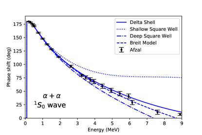
Figure 1: (Color online) Phase shifts of $\alpha-\alpha$ scattering in the $s$ wave, as a function of the energy in the laboratory frame computed with a shallow square-well potential (dotted line), the $\delta$-shell (solid line), the Breit model (dashed line) and a deep square well (dashed-dotted line). Data taken from Refs. Heydenburg and Temmer (1956); Afzal et al. (1969).

We adjust the parameters of the $\delta$-shell potential to the resonance energy and width and computed the resulting phase shifts. Figure 2 shows the phase shifts predicted from our approach. The central line is obtained from adjusting to the resonance energy and the central value of its width. Varying the resonance width $\Gamma=5.57\pm 0.25$ eV within its uncertainty produces the dark band. The systematic uncertainty estimate, i.e. the range that different models would explore, is shown as a light band. Its extent is generated by employing $\lambda(k)=\lambda_{0}\pm Rk^{4}/\Lambda_{b}^{2}$. We see that the prediction of the $\delta$-shell potential agrees well with data, even for energies beyond $E_{m}=1.7$ MeV. This model happens to be accurate.

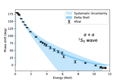
Figure 2: (Color online) Phase shifts of $\alpha-\alpha$ scattering in the $s$ wave, as a function of the energy in the center-of-mass frame. The dark band shows the uncertainty from the resonance width. The light band shows the theoretical uncertainty estimate. Data taken from Refs. Heydenburg and Temmer (1956); Afzal et al. (1969).

We computed the scattering length and effective range and obtained $a_{0}=-2020\pm 100$ fm and $r_{0}=1.106\pm 0.005$ fm, respectively. The uncertainties stem from the uncertainty in the resonance width. Let us compare this with effective range parameters from the literature. Overall, there is a consensus on the effective range, which is close to the estimate $1/(3k_{c})=1.21$ fm shown in Table 1. The scattering length, of course, is sensitive to the precise difference $r_{0}-1/(3k_{c})$ [see the approximation (7)], and it is probably only known to about 5 to 10%. The effective range expansions by Rasche (1967), Higa et al. (2008), and Kamouni and Baye (2007) found $a_{0}=1650\pm 150$ fm, $a_{0}=1920\pm 90$ fm, and $a_{0}=2390$ fm, respectively. The potential models by Kulik and Mur (2003) yielded $a_{0}=2030\pm 100$ fm. Ab initio computations have not yet reached the precision to extract very large scattering lengths precisely Elhatisari et al. (2015).

Kulik and Mur (2003) uses simple models for the computation of phase shifts and effective range parameters. The two-parameter models are (i) the $\delta$-shell potential, and (ii) the Breit model Breit and Bouricius (1948), i.e. a hard-core potential where the wave function’s logarithmic derivative at the hard core is set. These models are adjusted to the resonance energy and to phase shifts, and they virtually agree with each other for energies in the center-of-mass system up to 2 MeV. They agree with data over an even wider range. Interestingly, these models yield an accurate description of the resonance width when adjusted to phase shifts. Kamouni and Baye (2007) use the resonating group method and R-matrix theory to extract an effective range expansion. This approach adjusts about two parameters in each partial wave.

Let us contrast our approach to the halo EFT work by Higa et al. (2008). That approach is based on a dimer formulation with contact interactions. At leading order (LO), a fit to the resonance energy and width yields phase shifts that agree with data only up to 0.3 MeV in the center-of-mass frame. At next-to-leading-order (NLO), three parameters are adjusted to the resonance energy, its width, and phase shifts. The resulting phase shifts clearly deviate from data above 0.7 MeV of center-of-mass energy. Figure 3 compares the EFT results at LO and NLO to models. The EFT results are not accurate. This is somewhat surprising, because the effective-range expansion by the same authors yielded phase shifts that agree with data.

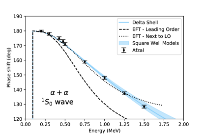
Figure 3: (Color online) Phase shifts of $\alpha+\alpha$ scattering in the $s$ wave computed from finite-range models and in leading order (LO) and next-to-leading order (NLO) Coulomb halo EFT Higa et al. (2008), as a function of the energy in the laboratory frame. Data taken from Refs. Heydenburg and Temmer (1956); Afzal et al. (1969).

III.2 ¹⁷F as ${}^{16}\mbox{O}+p$

The ¹⁷F nucleus plays a role in nucleosynthesis. Its $J^{\pi}=5/2^{+}$ ground state and its first excited $1/2^{+}$ states are bound by about 0.6 and 0.1 MeV, respectively. These energies are small compared to 6 MeV, the energy it takes to excite the doubly-magic nucleus ¹⁶O, and we can thus approximate ¹⁷F as a ${}^{16}\mbox{O}+p$ system at sufficiently low energies. The next excited states in ¹⁷F with quantum numbers $5/2^{+}$ and $1/2^{+}$ are separated by 6.7 and 6.5 MeV, respectively, from the corresponding bound states. Thus, the empirical breakdown energy is about $E_{b}\approx 6$ MeV. The sum of the charge radii of the proton and ¹⁶O is about $D\approx 3.6$ fm. This sets the theoretical breakdown momentum to $\pi/D\approx 0.88$ fm^-1, corresponding to an energy of about 17 MeV. Thus, the breakdown scale is set by the empirical breakdown energy. The Coulomb momentum is $k_{c}\approx 0.26$ fm^-1. Thus, potentials with a physical range $D$ are expected to exhibit model dependencies above about $\Lambda_{m}=(2k_{c}/D)^{1/2}\approx 0.27$ fm^-1, corresponding to an energy $E_{m}\approx 1.6$ MeV.

Let us consider the excited $J^{\pi}=1/2^{+}$ halo state Morlock et al. (1997). We adjust the model parameters to the binding energy and the ${}^{2}S_{1/2}$ phase shift data from Ref. Dubovichenko et al. (2017). The results are shown in Fig. 4. We then predict the ANC to be $C_{0}=78.9\pm 4.2$ fm^-1/2, and the charge radius of the excited state is $R^{*}_{c}=3.096\pm 0.034$ fm. The ANC agrees with the results by Gagliardi et al. (1999), Artemov et al. (2009), and Huang et al. (2010), who found values of ($80.6\pm 4.2$) fm^-1/2, ($75.5\pm 1.5$) fm^-1/2, and 77.2 fm^-1/2, respectively. Our effective range parameters are $a_{0}=4080\pm 430$ fm, and $r_{0}=1.17\pm 0.01$ fm. Within their uncertainties, these values agree with those of Refs. Kamouni and Baye (2007); Yarmukhamedov and Baye (2011).

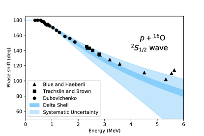
Figure 4: (Color online) Phase shifts of $p+^{16}\mbox{O}$ scattering in the ${}^{2}S_{1/2}$ partial wave, as a function of the energy in the center-of-mass frame. Data taken from Ref. Blue and Haeberli (1965); Trächslin and Brown (1967); Dubovichenko et al. (2017).

Let us also compare to Coulomb halo EFT. For the excited $1/2^{+}$ state, Ryberg et al. (2014a) employed one parameter at leading order and found that the relative distance $\langle r^{2}\rangle=(0.59~{}\mbox{fm})^{2}$ between the proton and the core and the ANC $C_{0}=21.4$ fm^-1/2 are too small. At next-to-leading order, effective range contributions enter, and the charge radius is increased by a factor 3.6–3.8 Ryberg et al. (2016).

Let us turn to the ¹⁷F ground state. Its charge radius is not yet known but its measurement is currently an active experiment at CERN Isolde Garcia Ruiz et. al (2016). We want to make a prediction for this observable. To put things into perspective we note that the charge radius of ¹⁹F is $R_{c}=2.8976(25)$ fm Angeli and Marinova (2013); the ground-state of that nucleus has spin/parity ${1/2}^{+}$. We adjust our model parameters to the binding energy and the ANC. The ground-state ANC extracted from transfer reaction data via potential models is $1.04\pm 0.05$ fm^-1/2 Gagliardi et al. (1999); Artemov et al. (2009). The resulting phase shifts are shown in Fig. 5. Unfortunately, the phase shift analysis lacks uncertainties, but we see a systematic deviation. We compute a scattering length of $a_{2}=1.15(11)\times 10^{3}$ fm⁵ and an effective range of $r_{2}=-0.068(7)$ fm^-3, in agreement with results by Yarmukhamedov and Baye (2011) (who were also informed by the ANCs we used). We compute a charge radius of $R_{c}=2.88(1)$ fm. This is a large radius for a $d$-wave state and practically as large as the charge radius of the $1/2^{+}$ ground state of ¹⁹F.

To estimate the reliability of our computations, we alternatively fit to the potential parameters to the phase shifts and the binding energy and find $R\approx 2.957$ fm and $\lambda_{0}\approx-1.924$ fm^-1. We note the the resulting $\chi^{2}$ per degree of freedom is about 11, hinting at phase-shift uncertainties of about three degrees (assuming them to be of statistical nature). In this case, we compute an ANC of $C_{2}=0.7286$ fm^-1/2, and a charge radius $R_{c}=2.80(2)$ fm. These values are significant smaller than those given in the previous paragraph, and the uncertainties do not overlap. It seems to us that the phase shift data Blue and Haeberli (1965); Trächslin and Brown (1967); Dubovichenko et al. (2017) and the transfer reaction data Gagliardi et al. (1999) are probably not compatible. We note, however, that the accurate determination of $d$-wave phase shifts from low-energy scattering is complicated because $s$ and $p$ waves dominate. We also note that somewhat smaller ANCs of 0.91 and 0.88 fm^-1/2 have been computed by Huang et al. (2010) and Blokhintsev et al. (2018), respectively. As the extraction of the ANC by Gagliardi et al. (1999) is more recent than the phase shift analysis (and includes uncertainties), we base our computation on the ANC and predict a charge radius of 2.88(1) fm for ¹⁷F. The measurement Garcia Ruiz et. al (2016) will certainly be useful to yield insight into the low-energy properties of the $p+\mbox{${}^{16}$O}$ system. We also note that this nucleus is in reach of ab initio computations Hagen et al. (2010), but its charge radius and ANC have not been computed, yet.

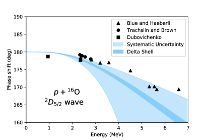
Figure 5: (Color online) Phase shifts of $p+^{16}\mbox{O}$ scattering in the ${}^{2}D_{5/2}$ partial wave, as a function of the energy in the center-of-mass frame. Data taken from Refs. Blue and Haeberli (1965); Trächslin and Brown (1967); Dubovichenko et al. (2017).

III.3 ⁶Li as a $\alpha+d$ bound state

The ground state of ⁶Li is only bound by about $E=1.47$ MeV with respect to the $d+\alpha$ threshold. This corresponds to a bound-state momentum of $\gamma\approx 0.31$ fm^-1. Its spin/parity is identical to that of the deuteron, and the estimate (5) for its magnetic moment yields $0.86$ nuclear magnetons, which is close to the observed value of $0.822$ Stone (2014). These basic properties suggest that the ⁶Li ground state exhibits a dominant $s$-wave halo structure, and we will we neglect any $d$ wave component in what follows.

Let us assess the breakdown scale. The three-body breakup of ⁶Li into $\alpha+n+p$ requires the breakup of the deuteron and is thus about 2.2 MeV above threshold. This inelastic process is without concern to us. The first excited state with the same spin and parity as the ground state is at 5.65 MeV, and this is the empirical breakdown energy. The sum of charge radii is $D\approx 3.8$ fm, setting the theoretical breakdown momentum at $\pi/D\approx 0.82$ fm^-1, which corresponds to a high energy of 10.6 MeV. Thus, the breakdown scale is set by the empirical properties. The binding energy of the deuteron to the $\alpha$ core is a factor of about four smaller than the breakdown energy, and this provides us with a separation of scale. The Coulomb momentum of the $d+\alpha$ system is $k_{c}\approx 0.09$ fm^-1, and model differences are start to get resolved above the momentum $\Lambda_{m}\approx 0.22$ fm^-1, corresponding to an energy $E_{m}\approx 0.75$ MeV. As this energy is smaller than the binding energy of the $\alpha+d$ system, model dependencies could be relevant. However, below we will see that the $\delta$-shell model yields an accurate description of existing low-energy data.

We model the ⁶Li ground state using the $\delta$-shell potential in the $s$ partial wave. Ryberg et al. (2014b) pointed out that charge radii can be used to constrain low-energy observables that are relevant in astrophysics. Together with the binding energy, these are the most precise data available at low energies. We therefore adjust the two parameters of our potential to the binding energy and the charge radius. The charge radius of ⁶Li is $2.589\pm 0.039$ fm Angeli and Marinova (2013) and we perform a total of three calculations, adjusting to its central, lower, and upper values. For the relevant $s$ wave we compute an ANC of $C_{0}=2.23(11)$ fm^-1/2, a scattering length $a_{0}=29.1\pm 1.7$ fm, and an effective range $r_{0}=1.85(5)$ fm. The uncertainties reflects the uncertainty in the charge radius. The central value of the inter-ion distance is $\sqrt{\langle r^{2}\rangle}=3.86$ fm, and this marginally exceeds the sum of charge radii of its constituents, 3.82 fm. The resulting phase shifts are shown in Fig. 6, and they agree with data Keller and Haeberli (1970); Grüebler et al. (1975). This gives us confidence in the accuracy of our results.

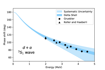
Figure 6: (Color online) Phase shifts of $d+\alpha$ scattering in the ${}^{3}S_{1}$ partial wave, as a function of the energy in the center-of-mass frame. Data taken from Refs. Keller and Haeberli (1970); Grüebler et al. (1975).

It is interesting to compare our prediction for the ANC and the effective range parameters with the literature. The effective range parameters agree with Ref. Krasnopol’sky et al. (1991), which states $a_{0}=30.8$ fm and $r_{0}=1.88$ fm; the ANC agrees with the values of Refs. Mukhamedzhanov et al. (2011); Blokhintsev and Savin (2014); Grassi et al. (2017). However, we note that ANCs have clearly evolved (and decreased) over time, as the papers Blokhintsev et al. (1993, 2006); Mukhamedzhanov et al. (2011); Tursunov et al. (2015) show. We note that the ab initio computation by Nollett et al. (2001) reports an ANC of $2.28\pm 0.02$ fm^-1/2 (in agreement with recent cluster models and our result), while Hupin et al. (2015) found a larger ANC of about $2.7$ fm^-1/2. While the calculation of Ref. Nollett et al. (2001) is informed by charge radii through its variational wave function, the paper Hupin et al. (2015) did not present results for charge radii. We believe our calculations, through their consistency for all low-energy observables, add further weight to an ANC around 2.2 fm^-1/2.

III.4 ⁷Be as $\alpha+^{3}\mbox{He}$ bound state

The ⁷Li ground state has quantum numbers $J^{\pi}=3/2^{-}$ and is bound by 1.6 MeV with respect to the $\alpha+\mbox{${}^{3}$He}$ threshold. The only other bound state is at about 0.4 MeV of excitation energy and has quantum numbers $J^{\pi}=1/2^{-}$. Both states are thus weakly bound and can be viewed as $p$ waves of the $\alpha+\mbox{${}^{3}$He}$ system. We note that the estimate (5) for the ground state’s magnetic moment, $-1.556$ nuclear magnetons, is close to the experimental value of $-1.398$ Stone (2014). This all suggests that we can describe ⁷Be as an $\alpha+^{3}\mbox{He}$ system.

The empirical breakdown energy is set by the energy of excited states 9.9 MeV for quantum numbers $J^{\pi}=3/2^{-}$; it is about twice as high for the numbers $J^{\pi}=1/2^{-}$ state. Of course, the ³He nucleus breaks up at an excitation energy of about 6 MeV, but this inelastic channel is of no concern for us. The sum of the two charge radii is $D\approx 3.6$ fm, setting the theoretical breakdown momentum to $\pi/D\approx 0.86$ fm^-1, corresponding to an energy of 9 MeV. Thus the breakdown energy is about 9 MeV. Model dependencies become visible above the momentum scale $\Lambda_{m}\approx 0.36$ fm^-1, corresponding to an energy of 1.6 MeV. We note that this energy is similar to the ground-state energy.

For the ${}^{2}P_{3/2}$ partial wave, we adjust the two parameters of the $\delta$-shell potential to the binding energy of the ground state and its charge radius of $2.646\pm 0.016$ fm Angeli and Marinova (2013). As before, we propagate the uncertainty of the charge radius to low-energy observables. Then, the ground-state ANC is $C_{1}=3.6\pm 0.1$ fm^-1/2, and the effective-range parameters are $a_{1}=207\pm 8$ fm³ and $r_{1}=-0.041\pm 0.004$ fm^-1. The predicted phase shifts are shown in Fig. 7 and compared to data  Spiger and Tombrello (1967); Boykin et al. (1972). The agreement is fair. Unfortunately, the older data by Spiger and Tombrello (1967) lacks uncertainties.

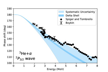
Figure 7: (Color online) Phase shifts of ${}^{3}\mbox{He}+\alpha$ scattering in the ${}^{2}P_{3/2}$ partial wave, as a function of the energy in the center-of-mass frame. Data taken from Refs. Spiger and Tombrello (1967); Boykin et al. (1972)

Let us compare with other approaches for the $3/2^{-}$ partial wave. Descouvemont et al. (2004) found an ANC of $C_{1}=3.79$ fm^-1/2 (close to our value) from an R matrix analysis, while Tursunmahatov and Yarmukhamedov (2012) found an ANC of $C_{1}=4.83^{+0.1}_{-0.25}$ from evaluations of capture reactions. We refer to the latter paper for a review of literature values. The ab initio computation by Dohet-Eraly et al. (2016) found a scattering volume of $a_{1}=210.4$ fm³ (close to our result), while the effective range expansion techniques Yarmukhamedov and Baye (2011) found effective range parameters $a_{1}=301\pm 6$ fm³ and $r_{1}=−0.0170\pm 0.0026$ fm^-1 (and a squared ANC of $C_{1}^{2}=23.3$ fm^-1). We note that the ab initio computation Dohet-Eraly et al. (2016) yields a charge radius that is close to data.

We note that Coulomb halo EFT was very recently applied to the $\alpha+\mbox{${}^{3}$He}$ system Higa et al. (2018); Zhang et al. (2018) for a computation of the astrophysical S factor. Zhang et al. (2018) pursued a Bayesian approach based on data from capture reactions, avoiding the need to adjust parameters to phse shifts. Higa et al. (2018) employed the ANC from Ref. Tursunmahatov and Yarmukhamedov (2012) for their computation of the astrophysical S factor. At leading order (a one-parameter or a three-parameter theory, depending on the power counting), the resulting phase shifts are visibly above the data Boykin et al. (1972).

It seems to us that this $\alpha+\mbox{${}^{3}$He}$ system is still not sufficiently well understood. Existing theoretical results are in conflict with each other, and no calculation seems to be able to reproduce charge radii, phase shifts, and capture data.

III.5 ⁷Li as $\alpha+\mbox{${}^{3}$H}$ bound state

The $3/2^{-}$ ground state of ⁷Li is bound by about 2.5 MeV with respect to the threshold of the $\alpha+\mbox{${}^{3}$H}$ system. Based on a cluster assumption (5), its magnetic moment is 3.4 nuclear magnetons, which is close to the experimental datum of 3.256 Stone (2014). This suggests that one can describe ⁷Li as the bound state of the $\alpha+\mbox{${}^{3}$H}$ system with orbital angular momentum $l=1$.

The next $3/2^{-}$ state is at about 9.8 MeV, setting the empirical breakdown scale. The breakup of the triton at about 6 MeV is an inelastic channel we are not concerned with. The sum of the charge radii of the constituent ions is $D\approx 3.4$ fm, and the theoretical breakdown momentum is $\pi/D\approx 0.91$ fm^-1, corresponding to an energy of about 10 MeV. Thus the breakdown energy is at about 10 MeV. At the momentum $\Lambda_{m}=0.26$ fm^-1, corresponding to an energy of 0.84 MeV, model dependencies become visible. We note that this energy is smaller than the bound-state energy, and model dependencies could thus be notable.

We adjust the $\delta$-shell parameters to the $\alpha$-separation energy and the charge radius ($2.444\pm 0.042$ fm Angeli and Marinova (2013)) of the ⁷Li. The resulting phase shifts are shown in Fig. 8 and compared to a phase shift analysis Spiger and Tombrello (1967). The agreement is poor. However, the scatter of the points from the phase shift analysis also suggests that the uncertainties are significant.

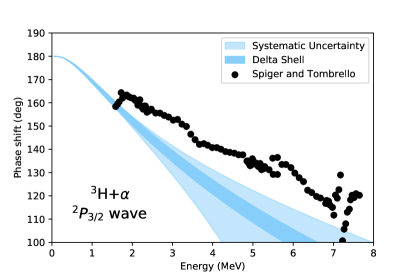
Figure 8: (Color online) Phase shifts of $\mbox{${}^{3}$H}+\alpha$ scattering in the ${}^{2}P_{3/2}$ partial wave, as a function of the energy in the center-of-mass frame. Data taken from Ref. Spiger and Tombrello (1967).

For the $3/2^{-}$ channel, we compute a scattering volume $a_{1}=74\pm 8$ fm³, an effective range $r_{1}=-0.24\pm 0.02$ fm^-1, and an ANC $C_{1}=3.0\pm 0.2$ fm^-1/2. The ab initio computations by Dohet-Eraly et al. (2016) found a scattering volume of 70 fm³ (which agrees with our result), and their computed charge radius is close to data. Kamouni and Baye (2007) fit a model to phase shifts and report effective-range parameters $a_{1}=72.77$ fm³ and $r_{1}=−0.27$ fm^-1 (which are close to our results); however, the ground-state energy of the ${}^{3}\mbox{H}+\alpha$ system was about twice as large as the data. However, Descouvemont et al. (2004) found an ANC of $C_{1}=3.49$ fm^-1/2 from an R matrix analysis, while Yarmukhamedov and Baye (2011) computed effective-range parameters $a_{1}=58.10\pm 0.65$ fm³ and $r_{1}=−0.346\pm 0.005$ fm^-1 (with an ANC of $C_{1}=3.57\pm 0.15$ from Ref. Igamov and Yarmukhamedov (2007)).

We see that there is no consensus yet about low-energy observables for the $\alpha+\mbox{${}^{3}$H}$ system. However, the simplicity of the $\delta$-shell potential, its economical use of only two low-energy data, its agreement with ab initio computations, and its ability to estimate uncertainties of models make it an attractive potential also here.

IV Summary

We employed a simple two-parameter model to describe a number of nuclear light-ion systems that exhibit a separation of scale. Whenever possible, the model parameters were constrained by the energy and width of a low-energy resonance or by the energy and charge radius of a weakly bound state. In those cases, we predicted phase shifts, effective range parameters and ANCs. Our analysis of ANCs, charge radii and resonance widths shows that the inclusion of a finite range is relevant for systems with strong Coulomb interactions. We also proposed a way to account for systematic corrections and model uncertainties. This allowed us to present uncertainty estimates for the computed observables. The presented approach provides us with a constructive criticism of Coulomb halo EFT. We predicted a charge radius of $2.88(1)$ fm for the ¹⁷F ground state, taking its energy and ANC to constrain the model.

The potential model employs two parameters in each partial wave. When applied to a single partial wave, it is a minimal model whose results compete well at low energies with traditional Woods-Saxon potential models or $R$ matrix analyses that employ more parameters. We pointed out that the $\delta$-shell model practically delivers model-independent results below a momentum $\Lambda_{m}$ when it is adjusted to low-energy data. We also presented simple formulas that estimate the sizes of effective-range parameters and ANCs based on energies of low-energy states and charge radii of the involved ions. Such estimates are useful in the construction of EFTs, and they seemed to be missing in the literature.

V Appendix

The Appendix presents some details that could be looked up or are straightforward (but sometimes tedious) to derive. We present them here briefly to make the paper self contained.

V.1 Coulomb wave function

For the Coulomb wave functions we followed Gaspard and Sparenberg (2018). In that paper, the analytical properties are emphazised. This is relevant to us because we call the Coulomb wave functions at real and purely imaginary arguments. We employed Mathematica and scipy special functions in Python for our numerical implementation. We checked for a number of arguments that our implementation agrees with the precise numerical routines by Michel (2007).

The regular Coulomb wave function is

$$F_{l}(\eta,\rho)=C_{l}(\eta)\rho^{l+1}e^{i\rho}M(l+1+i\eta,2l+2,-i2\rho).$$

Here, $\eta=k_{c}/k$ is the Sommerfeld parameter, and $\rho=kr$. For bound states with energy $E=-\hbar^{2}\gamma^{2}/(2m)$ we have $k=-i\gamma$, and the arguments $\eta=-ik_{c}/\gamma$, and $\rho=i2\gamma r$ are purely imaginary. In Eq. (V.1), we employed Kummer’s function $M(a,b,z)$, or the confluent hypergeometric function ${{}_{1}F_{1}}(a,b,z)=M(a,b,z)$. The $\eta$-dependent normalization $C_{l}(\eta)$, distinct from the ANC by its argument, is

$$C_{l}(\eta)=\frac{(2\eta)^{l}}{(2l+1)!}\sqrt{\frac{2\pi\eta w_{l}(\eta)}{e^{2\pi\eta}-1}},$$ (48)

with

$$w_{l}(\eta)=\prod_{j=0}^{l}\left(1+{j^{2}\over\eta^{2}}\right).$$ (49)

The incoming and outgoing Coulomb wave functions are

$$H^{\pm}_{l}(\eta,\rho)=D^{\pm}_{l}(\eta)\rho^{l+1}e^{\pm i\rho}U(l+1\pm i\eta,2l+2,\mp i2\rho).$$

Here, $U$ denotes Tricomi’s function (or the confluent hypergeometric function of the second kind) and the normalization is

$$D^{\pm}_{l}(\eta)=\mp i2(-1)^{l}e^{\pi\eta}\frac{(2l+1)!C_{l}(\eta)}{\Gamma(l+1\mp i\eta)}.$$ (51)

The irregular Coulomb wave function is then defined as

$$G_{l}(\eta,\rho)={1\over 2}\left[H^{+}_{l}(\eta,\rho)+H^{-}_{l}(\eta,\rho)\right].$$ (52)

We are interested in low-energy phenomena and therefor seek approximations for Coulomb wave functions for $\eta\gg 1$. Following (DLMF, , Chapter 33.9) we expand the Coulomb wave functions into a series of modified Bessel functions whose coefficients decrease with inverse powers of $\eta$. Thus, ($\eta\equiv k_{c}/k$ and $\rho\equiv kR$)

$$F_{0}(\eta,\rho) = {C_{0}(\eta)\over 2\eta}\sum_{n=1}^{\infty}b_{n}(2k_{c}R)^{n\over 2}I_{n}(2\sqrt{2k_{c}R}),$$

$$G_{0}(\eta,\rho) = {2\over\beta_{0}(\eta)C_{0}(\eta)}\sum_{n=1}^{\infty}(-1)^{n}b_{n}(2k_{c}R)^{n\over 2}K_{n}(2\sqrt{2k_{c}R})$$

. (53)

Here,

$$b_{1} = 1,$$

$$b_{2} = 0,$$

$$b_{3} = -{1\over 4\eta^{2}},$$

$$b_{4} = -{1\over 12\eta^{2}},$$ (54)

and all other $b_{n}$ are of order ${\cal O}(\eta^{-4})$ or smaller. We have

$$\beta_{0}(\eta)=-1+{\cal O}(\eta^{-4}).$$ (55)

Similar expressions exist for nonzero orbital angular momentum.

We also need to know similar approximations for the Coulomb wave functions for purely imaginary momentum $k=i\gamma$. In the weak-binding limit $\gamma\to 0$, the regular Coulomb wave function becomes (DLMF, , Eq. 13.8.12)

$$F_{l}\left({k_{c}\over i\gamma},i\gamma r\right)\approx$$ (56)

$$(i\gamma r)^{l+1}C_{l}(-ik_{c}/\gamma)\frac{(2l+1)!}{(2k_{c}r)^{l+1/2}}I_{2l+1}(2\sqrt{2k_{c}r}).$$

The Coulomb wave functions $G_{l}$ and $H^{+}_{l}$ are based on Tricomi’s function. For $\gamma\to 0$ we use (see Ref. Abramowitz and Stegun (1964))

$$\lim_{a\to\infty}U(a,b,z/a)\Gamma(1+a-b)=2z^{{1-b\over 2}}K_{b-1}(2\sqrt{z}).$$

We see that Coulomb wave functions are approximated by modified Bessel functions as the momentum goes to zero. Let us also consider approximations of the latter. We have

$$I_{n}(z) \approx \left({z\over 2}\right)^{n}\left({1\over n!}+{z^{2}\over 4(n+1)!}\right),$$

$$K_{n}(z) \approx {1\over 2}\left({2\over z}\right)^{n}\left((n-1)!+{(n-2)!z^{2}\over 4}\right),$$

valid for $z\ll 1$, see (DLMF, , Chapters 10.25 and 10.31). We also have

$$I_{n}(z) \approx {e^{z}\over\sqrt{2\pi z}}\left(1-{a_{1}(n)\over z}\right),$$

$$K_{n}(z) \approx \sqrt{\pi\over 2z}e^{-z}\left(1+{a_{1}(n)\over z}\right),$$

valid for $z\to\infty$, see (DLMF, , Chapter 10.40). Here,

$$a_{1}(n)\equiv{4n^{2}-1\over 8}.$$ (60)

V.2 Estimate for the asymptotic normalization coefficient and inter-ion distance

We want to compute an estimate for the ANC. For the $\delta$-shell potential, the bound-state wave function can be written as follows.

$$u_{l}(r)=\left\{\begin{array}[]{ll}C_{l}\frac{W_{-{k_{c}\over\gamma},l+{1\over 2}}(2\gamma R)}{F_{l}\left({k_{c}\over i\gamma},i\gamma R\right)}F_{l}\left({k_{c}\over i\gamma},i\gamma r\right)&\mbox{, for $r<R$,}\\ C_{l}W_{-{k_{c}\over\gamma},l+{1\over 2}}(2\gamma r)&\mbox{, for $r>R$.}\end{array}\right.$$ (63)

Here, we employed the Whittaker function $W$ (which is proportional to the outgoing Coulomb wave function for bound states DLMF ), and $C_{l}$ is the ANC by definition. We have

$$W_{\kappa,\mu}(z)=e^{-{z\over 2}}z^{\mu+{1\over 2}}U({1/2}+\mu-\kappa,1+2\mu,z)$$ (64)

The ANC is determined by the normalization condition

$$1 = \int\limits_{0}^{\infty}dr\left|u_{l}(r)\right|^{2}$$ (65)

$$= C_{l}^{2}\int\limits_{R}^{\infty}dr\left(W_{-{k_{c}\over\gamma},l+{1\over 2}}(2\gamma r)\right)^{2}$$

$$+\left|C_{l}\frac{W_{-{k_{c}\over\gamma},l+{1\over 2}}(2\gamma R)}{F_{l}\left({k_{c}\over i\gamma},i\gamma R\right)}\right|^{2}\int\limits_{0}^{R}dr\left|F_{l}\left({k_{c}\over i\gamma},i\gamma r\right)\right|^{2}.$$

To perform the integration, we need to make approximations. As we are interested in the case of weak binding, i.e. $\gamma\to 0$, we use the approximation (V.1). Thus,

$$W_{-{k_{c}\over\gamma},l+{1\over 2}}(2\gamma r) \approx \frac{2(2k_{c}r)^{-l-{1\over 2}}}{\Gamma(k_{c}/\gamma-l)}K_{2l+1}\left(2\sqrt{2k_{c}r}\right).$$ (66)

Here, we approximated $e^{-\gamma r}\approx 1$. We note that the bound-state momentum enters as the argument of the $\Gamma$ function. To simplify matters further, we approximate

$$\Gamma(k_{c}/\gamma-l)\left({k_{c}\over\gamma}\right)^{l+1}\approx\Gamma(k_{c}/\gamma+1),$$ (67)

which is correct in leading order when $\gamma\ll k_{c}$. Then

$$W_{-{k_{c}\over\gamma},l+{1\over 2}}(2\gamma r) \approx \frac{2\sqrt{2k_{c}r}}{\Gamma(1+k_{c}/\gamma)}K_{2l+1}\left(2\sqrt{2k_{c}r}\right).$$ (68)

In the weak-binding limit $\gamma\to 0$, we use the approximation (56) for the regular Coulomb wave function. The integral (65) can now be evaluated exactly (e.g. via Mathematica), but we did not find the result particularly illuminating. However, for $l=0$ one can then take the limit $R\to 0$ and finds

$$C_{0}\approx\sqrt{6k_{c}}\Gamma(1+k_{c}/\gamma).$$ (69)

This is the result from leading-order Coulomb halo EFT Ryberg et al. (2016).

For further analytical insights we return to Eqs. (68) and (56), and assume $k_{c}R\gg 1$. This allows us to use the leading terms of Eqs. (V.1). We change the integration variable to $z=\sqrt{2k_{c}r}$ and perform the integration (65). Keeping only the leading term in $k_{c}R\gg 1$ yields

$$C_{l}\approx{\Gamma(1+k_{c}/\gamma)\over\sqrt{\pi R}}e^{2\sqrt{2k_{c}R}}.$$ (70)

Replacing $R\to D$ yields the result presented in Table 1.

Similar computations allow us also to give an estimate for the squared inter-ion distance (21). Making the same approximations as in the computation of the ANC we find (for orbital angular momentum $l=0$)

$$\langle r^{2}\rangle\approx\left\{\begin{array}[]{ll}{9\over 35}k_{c}^{-2},&\mbox{for $R\to 0$, }\\ R^{2},&\mbox{for $k_{c}R\gg 1$.}\end{array}\right.$$ (73)

The results are strikingly different from each other because the wave function is strongly localized and peaked around $r=R$ in for large Coulomb momenta. We see in particular that the inter-ion distance does not depend on the bound-state momentum, and this is in stark contrast to the case without Coulomb, where $\langle r^{2}\rangle\propto\gamma^{-2}$. Replacing $R\to D$ yields the expressions presented in Table 1.

V.3 Estimate for the resonance width

For the $\delta$-shell potential, the resonance width is given in Eq. (34).

Using the approximation (V.1) the inverse width becomes in leading order of $k_{c}/\kappa\gg 1$

$${E\over\Gamma} \approx {\kappa R\over 3C_{0}^{2}(\eta)}\frac{\sqrt{2k_{c}R}(I_{1}K_{4}-I_{4}K_{1})-3(I_{1}K_{3}+I_{3}K_{1})}{I_{1}^{2}}$$

. (74)

Here, we have suppressed the arguments of the modified Bessel function, i.e. $I_{n}\equiv I_{n}(2\sqrt{2k_{c}R})$ and $K_{n}\equiv K_{n}(2\sqrt{2k_{c}R})$.

We consider two cases. For zero-range interactions, we take $R\to 0$ and obtain

$${\Gamma\over E}\bigg{|}_{R\to 0}\approx 24\pi{k_{c}^{2}\over\kappa^{2}}e^{-2\pi{k_{c}\over\kappa}}.$$ (75)

Here, we used the expansions (V.1). The physically relevant case $k_{c}R\gg 1$ is more interesting. We use the expansions (V.1) and find

$${\Gamma\over E}\bigg{|}_{k_{c}R\gg 1}\approx 4{k_{c}\over\kappa^{2}R}e^{4\sqrt{2k_{c}R}}e^{-2\pi{k_{c}\over\kappa}}.$$ (76)

Replacing $R\to D$ yields the results presented in Subsection II.1.

V.4 Estimates for effective-range parameters

We start from the effective-range parameters given in Eq. (II.2.2). These expressions contain the strength $\lambda_{0}$ of the $\delta$-shell potential. For a resonance with energy $E=\hbar^{2}\kappa^{2}/(2m)$ this parameter fulfills Eq. (31). We assume $\kappa\ll k_{c}$ and use the approximation (V.1), focusing on orbital angular momentum $l=0$. This yields

$$(\lambda_{0}R)^{-1}\approx-2I_{1}K_{1}-\frac{\kappa^{2}R}{8k_{c}\sqrt{2k_{c}R}},$$ (77)

and we have omitted higher-order corrections in $\kappa/k_{c}$. Here, and in what follows the modified Bessel functions have arguments $I_{n}\equiv I_{n}(2\sqrt{2k_{c}R})$ and similar for $K_{n}$.

We insert the expression (77) into the Eq. (II.2.2) for the $s$-wave scattering length and find

$$a_{0}^{-1}=-\frac{\kappa^{2}R}{4I_{1}^{2}\sqrt{2k_{c}R}}.$$ (78)

Again, we consider two approximations. For $2\sqrt{2k_{c}R}\gg 1$, we take the leading approximation of Eqs. (V.1) and find

$$a_{0} = -(\pi\kappa^{2}R)^{-1}e^{4\sqrt{2kc_{D}}}.$$ (79)

For $R\to 0$, we take the approximations (V.1) and find $a_{0}=-6k_{c}/\kappa^{2}$. Replacing $R\to D$ yields the expressions given in Table 1.

We turn to the effective range of Eq. (II.2.2) and employ the leading term $(\lambda_{0}R)^{-1}\approx-2I_{1}K_{1}$ from Eq. (77). This yields

$$r_{0}={1\over 3k_{c}}\left(1+\frac{2(2kcR)^{3/2}I_{2}K_{1}-k_{c}R}{I_{1}^{2}}\right).$$ (80)

Again, we consider two approximations. For $2\sqrt{2k_{c}R}\gg 1$, we take the Eqs. (V.1) and find Mur et al. (1993)

$$r_{0}=(3k_{c})^{-1}-\pi R\,e^{-4\sqrt{2k_{c}R}}.$$ (81)

For $R\to 0$, we employ the approximations (V.1) and find $r_{0}={\cal O}(R))$. Replacing $R\to D$ yields the expressions given in Table 1 and in Eq. (6).

V.5 Derivatives of Coulomb wave functions

We limit the discussion to orbital angular momentum $l=0$ and positive energies. For $k\ll k_{c}$ we find ($z\equiv 2\sqrt{2k_{c}r}$) from Eq. (V.1) that

$$F_{0}(k_{c}/k,kr) \propto zI_{1}(z),$$

$$G_{0}(k_{c}/k,kr) \propto zK_{1}(z).$$ (82)

Here, we neglected any constants and functions that depend on $k$ and $k_{c}$, but not on $r$. We see that only the combination $2k_{c}r$ enters, and it is clear that a derivative with respect to $r$ will yield a factor $k_{c}$ rather than $k$. Taking a derivative becomes particularly simple for strong Coulomb interactions as $k_{c}r\gg 1$ practically holds for all distances exceeding 1 fm or so. We use the approximations (V.1) and find

$$F_{0}(k_{c}/k,kr) \propto \sqrt{z\over 2\pi}e^{z},$$

$$G_{0}(k_{c}/k,kr) \propto \sqrt{\pi z\over 2}e^{-z}.$$ (83)

Taking the derivative with respect to $r$, and using $z\gg 1$ yields

$${d\over dr}F_{0}(k_{c}/k,kr) \approx +4k_{c}F_{0}(k_{c}/k,kr),$$

$${d\over dr}G_{0}(k_{c}/k,kr) \approx -4k_{c}G_{0}(k_{c}/k,kr).$$ (84)

V.6 Square well plus Coulomb

The potential is

$$V(r)=\left\{\begin{array}[]{ll}-{\hbar^{2}q^{2}\over 2m},&r<R\\ {Z_{1}Z_{2}\alpha\hbar\over r}&r>R.\end{array}\right.$$ (87)

We limit ourselves to $s$ waves. Solutions with positive energy $E=\hbar^{2}k^{2}/(2m)$ are

$$u(r)=$$ (90)

$$\left\{\begin{array}[]{ll}\frac{\cos\delta F_{0}\left({k_{c}\over k},kR\right)+\sin\delta G_{0}\left({k_{c}\over k},kR\right)}{\sin p_{k}R}\sin{p_{k}r},&r<R\\ \cos\delta F_{0}\left({k_{c}\over k},kr\right)+\sin\delta G_{0}\left({k_{c}\over k},kr\right),&r>R.\end{array}\right.$$

Here, $p_{k}\equiv\sqrt{k^{2}+q^{2}}$. The phase shifts fulfill

$$\cot\delta=$$ (91)

$$\frac{G^{\prime}_{0}\left({k_{c}\over k},kR\right)\sin{p_{k}R}-{p\over k}G_{0}\left({k_{c}\over k},kR\right)\cos{p_{k}R}}{F^{\prime}_{0}\left({k_{c}\over k},kR\right)\sin{p_{k}R}-{p_{k}\over k}F_{0}\left({k_{c}\over k},kR\right)\cos{p_{k}R}}$$

Here, we used $F^{\prime}_{0}(\eta,z)\equiv{d\over dz}F_{0}(\eta,z)$ and similar for the irregular Coulomb wave function. A resonance at energy $E_{\kappa}\equiv\hbar^{2}\kappa^{2}/(2m)$ fulfills

$$p_{\kappa}\cot{p_{\kappa}R}=\kappa\frac{G^{\prime}_{0}\left({k_{c}\over\kappa},\kappa R\right)}{G_{0}\left({k_{c}\over\kappa},\kappa R\right)}$$ (92)

The resonance width $\Gamma$ fulfills

$${E_{\kappa}\over\Gamma}= {G_{0}\over 4}\left({q^{2}\over p_{\kappa}^{2}}G_{0}^{\prime}+\kappa\dot{G}^{\prime}_{0}-\kappa{G^{\prime}_{0}\dot{G}_{0}\over G_{0}}+{\kappa RG_{0}\over\sin^{2}{p_{\kappa}R}}\right)$$

. (93)

Here, we used $\dot{G}_{0}(kc/\kappa,\kappa R)\equiv{d\over d\kappa}G_{0}(k_{c}/\kappa,\kappa R)$, and we dropped the arguments for all Coulomb wave function. For a given resonance energy and width, one can solve Eqs. (92) and (V.6) for the parameters $(q,R)$ of the potential. Once these are known, the phase shifts result from Eq. (91). As the square well can hold an arbitrary number of bound states, the solutions are not unique. However, low-energy data such as the $\alpha-\alpha$ phase shifts exhibit sensitivity to such details only at energies above about 1.7 MeV.

References

- Adelberger et al. (2011) E. G. Adelberger, A. García, R. G. Hamish Robertson, K. A. Snover, A. B. Balantekin, K. Heeger, M. J. Ramsey-Musolf, D. Bemmerer, A. Junghans, C. A. Bertulani, J.-W. Chen, H. Costantini, P. Prati, M. Couder, E. Uberseder, M. Wiescher, R. Cyburt, B. Davids, S. J. Freedman, M. Gai, D. Gazit, L. Gialanella, G. Imbriani, U. Greife, M. Hass, W. C. Haxton, T. Itahashi, K. Kubodera, K. Langanke, D. Leitner, M. Leitner, P. Vetter, L. Winslow, L. E. Marcucci, T. Motobayashi, A. Mukhamedzhanov, R. E. Tribble, Kenneth M. Nollett, F. M. Nunes, T.-S. Park, P. D. Parker, R. Schiavilla, E. C. Simpson, C. Spitaleri, F. Strieder, H.-P. Trautvetter, K. Suemmerer, and S. Typel, “Solar fusion cross sections. ii. the chain and cno cycles,” Rev. Mod. Phys. 83, 195–245 (2011).
- Buck et al. (1975) B. Buck, C. B. Dover, and J. P. Vary, “Simple potential model for cluster states in light nuclei,” Phys. Rev. C 11, 1803–1821 (1975).
- Kulik and Mur (2003) A. V. Kulik and V. D. Mur, “, 3he, and scattering in the vicinity of the 5he∗ and 5li∗ resonances,” Phys. Atom. Nuclei 66, 87 (2003).
- Typel and Baur (2005) S. Typel and G. Baur, “Electromagnetic strength of neutron and proton single-particle halo nuclei,” Nuclear Physics A 759, 247 – 308 (2005).
- Grassi et al. (2017) A. Grassi, G. Mangano, L. E. Marcucci, and O. Pisanti, “ astrophysical factor and its implications for big bang nucleosynthesis,” Phys. Rev. C 96, 045807 (2017).
- Hamilton et al. (1973) J. Hamilton, I. Øverbö, and B. Tromborg, “Coulomb corrections in non-relativistic scattering,” Nuclear Physics B 60, 443 – 477 (1973).
- Mur and Popov (1985) V. D. Mur and V. S. Popov, “Coulomb problem with short-range interaction: Exactly solvable model,” Theoretical and Mathematical Physics 65, 1132–1140 (1985).
- Mur et al. (1993) V. D. Mur, B. M. Karnakov, S. G. Pozdnyakov, and V. S. Popov, “Low-energy parameters of the dt and d3He systems,” Physics of Atomic Nuclei 56, 217–226 (1993).
- Sparenberg et al. (2010) Jean-Marc Sparenberg, Pierre Capel, and Daniel Baye, “Influence of low-energy scattering on loosely bound states,” Phys. Rev. C 81, 011601 (2010).
- Yarmukhamedov and Baye (2011) R. Yarmukhamedov and D. Baye, “Connection between effective-range expansion and nuclear vertex constant or asymptotic normalization coefficient,” Phys. Rev. C 84, 024603 (2011).
- Ramírez Suárez and Sparenberg (2017) O. L. Ramírez Suárez and J.-M. Sparenberg, “Phase-shift parametrization and extraction of asymptotic normalization constants from elastic-scattering data,” Phys. Rev. C 96, 034601 (2017).
- Blokhintsev et al. (2018) L. D. Blokhintsev, A. S. Kadyrov, A. M. Mukhamedzhanov, and D. A. Savin, “Extrapolation of scattering data to the negative-energy region. iii. application to the system,” Phys. Rev. C 98, 064610 (2018).
- Higa et al. (2008) R. Higa, H.-W. Hammer, and U. van Kolck, “ scattering in halo effective field theory,” Nuclear Physics A 809, 171 – 188 (2008).
- Ryberg et al. (2014a) Emil Ryberg, Christian Forssén, H.-W. Hammer, and Lucas Platter, “Effective field theory for proton halo nuclei,” Phys. Rev. C 89, 014325 (2014a).
- Zhang et al. (2014) Shi-Sheng Zhang, M. S. Smith, Zhong-Shu Kang, and Jie Zhao, “Microscopic self-consistent study of neon halos with resonant contributions,” Phys. Lett. B 730, 30 – 35 (2014).
- Higa et al. (2018) Renato Higa, Gautam Rupak, and Akshay Vaghani, “Radiative 3he(,)7be reaction in halo effective field theory,” The European Physical Journal A 54, 89 (2018).
- Capel et al. (2018) P. Capel, D. R. Phillips, and H.-W. Hammer, “Dissecting reaction calculations using halo effective field theory and ab initio input,” Phys. Rev. C 98, 034610 (2018).
- Zhang et al. (2018) Xilin Zhang, Kenneth M. Nollett, and Daniel R. Phillips, “-factor and scattering parameters from 3He + 4He Be + data,” arXiv e-prints , arXiv:1811.07611 (2018), arXiv:1811.07611 [nucl-th] .
- Neff (2011) Thomas Neff, “Microscopic calculation of the and capture cross sections using realistic interactions,” Phys. Rev. Lett. 106, 042502 (2011).
- Nollett et al. (2001) K. M. Nollett, R. B. Wiringa, and R. Schiavilla, “Six-body calculation of the -deuteron radiative capture cross section,” Phys. Rev. C 63, 024003 (2001).
- Quaglioni and Navrátil (2008) Sofia Quaglioni and Petr Navrátil, “Ab Initio many-body calculations of , , , and scattering,” Phys. Rev. Lett. 101, 092501 (2008).
- Hupin et al. (2015) Guillaume Hupin, Sofia Quaglioni, and Petr Navrátil, “Unified description of structure and deuterium- dynamics with chiral two- and three-nucleon forces,” Phys. Rev. Lett. 114, 212502 (2015).
- Dohet-Eraly et al. (2016) Jérémy Dohet-Eraly, Petr Navrátil, Sofia Quaglioni, Wataru Horiuchi, Guillaume Hupin, and Francesco Raimondi, “He3be7 and h3li7 astrophysical s factors from the no-core shell model with continuum,” Physics Letters B 757, 430 – 436 (2016).
- Dubovichenko and Dzhazairov-Kakhramanov (2017) Sergey Dubovichenko and Albert Dzhazairov-Kakhramanov, “Study of the nucleon radiative captures 8li()9li, 9be()10b, 10be()11be, 10b()11c, and 16o()17f at thermal and astrophysical energies,” International Journal of Modern Physics E 26, 1630009 (2017).
- Descouvemont et al. (2004) Pierre Descouvemont, Abderrahim Adahchour, Carmen Angulo, Alain Coc, and Elisabeth Vangioni-Flam, “Compilation and r-matrix analysis of big bang nuclear reaction rates,” Atomic Data and Nuclear Data Tables 88, 203 – 236 (2004).
- Huang et al. (2010) J. T. Huang, C. A. Bertulani, and V. Guimarães, “Radiative capture of nucleons at astrophysical energies with single-particle states,” Atomic Data and Nuclear Data Tables 96, 824 – 847 (2010).
- Dobaczewski et al. (2014) J. Dobaczewski, W. Nazarewicz, and P.-G. Reinhard, “Error estimates of theoretical models: a guide,” Journal of Physics G: Nuclear and Particle Physics 41, 074001 (2014).
- Furnstahl et al. (2015) R. J. Furnstahl, D. R. Phillips, and S. Wesolowski, “A recipe for eft uncertainty quantification in nuclear physics,” Journal of Physics G: Nuclear and Particle Physics 42, 034028 (2015).
- Schindler and Phillips (2009) M. R. Schindler and D. R. Phillips, “Bayesian methods for parameter estimation in effective field theories,” Ann. Phys. 324, 682 – 708 (2009).
- Furnstahl et al. (2015) R. J. Furnstahl, G. Hagen, T. Papenbrock, and K. A. Wendt, “Infrared extrapolations for atomic nuclei,” Journal of Physics G: Nuclear and Particle Physics 42, 034032 (2015).
- Coello Pérez and Papenbrock (2015) E. A. Coello Pérez and T. Papenbrock, “Effective field theory for nuclear vibrations with quantified uncertainties,” Phys. Rev. C 92, 064309 (2015).
- Carlsson et al. (2016) B. D. Carlsson, A. Ekström, C. Forssén, D. Fahlin Strömberg, G. R. Jansen, O. Lilja, M. Lindby, B. A. Mattsson, and K. A. Wendt, “Uncertainty analysis and order-by-order optimization of chiral nuclear interactions,” Phys. Rev. X 6, 011019 (2016).
- Bedaque and van Kolck (2002) P. F. Bedaque and U. van Kolck, “Effective field theory for few-nucleon systems,” Annual Review of Nuclear and Particle Science 52, 339–396 (2002), nucl-th/0203055 .
- Bertulani et al. (2002) C. A. Bertulani, H.-W. Hammer, and U. van Kolck, “Effective field theory for halo nuclei: shallow p-wave states,” Nucl. Phys. A 712, 37 – 58 (2002).
- Hammer et al. (2017) H.-W. Hammer, C. Ji, and D. R. Phillips, “Effective field theory description of halo nuclei,” Journal of Physics G: Nuclear and Particle Physics 44, 103002 (2017).
- (36) T. Papenbrock, Talk at the workshop Progress in Ab Initio Techniques in Nuclear Physics, TRIUMF, Vancouver, B.C. (February 2019).
- Schmickler et al. (2019) C. H. Schmickler, H. W. Hammer, and A. G. Volosniev, “Universal physics of bound states of a few charged particles,” arXiv e-prints , arXiv:1904.00913 (2019), arXiv:1904.00913 [nucl-th] .
- Buck and Pilt (1977) B. Buck and A. A. Pilt, “Alpha-particle and triton cluster states in 19f,” Nuclear Physics A 280, 133 – 160 (1977).
- Ryberg et al. (2019) E. Ryberg, C. Forssén, D. R. Phillips, and U. van Kolck, “Finite-size effects in heavy halo nuclei from effective field theory,” arXiv e-prints , arXiv:1905.01107 (2019), arXiv:1905.01107 [nucl-th] .
- König et al. (2013) Sebastian König, Dean Lee, and H.-W. Hammer, “Causality constraints for charged particles,” Journal of Physics G: Nuclear and Particle Physics 40, 045106 (2013).
- Gagliardi et al. (1999) C. A. Gagliardi, R. E. Tribble, A. Azhari, H. L. Clark, Y.-W. Lui, A. M. Mukhamedzhanov, A. Sattarov, L. Trache, V. Burjan, J. Cejpek, V. Kroha, Š. Piskoř, and J. Vincour, “Tests of transfer reaction determinations of astrophysical s factors,” Phys. Rev. C 59, 1149–1153 (1999).
- Artemov et al. (2009) S. V. Artemov, S. B. Igamov, K. I. Tursunmakhatov, and R. Yarmukhamedov, “Determination of nuclear vertex constants (asymptotic normalization coefficients) for the virtual decays 3he d + p and 17f 16o + p and their use for extrapolating astrophysical s-factors of the radiative proton capture by the deuteron and the 16o nucleus at very low energies,” Bulletin of the Russian Academy of Sciences: Physics 73, 165–170 (2009).
- Breit and Bouricius (1948) G. Breit and W. G. Bouricius, “A boundary value condition for proton-proton scattering,” Phys. Rev. 74, 1546–1547 (1948).
- Kok et al. (1982) L. P. Kok, J. W. de Maag, H. H. Brouwer, and H. van Haeringen, “Formulas for the -shell-plus-coulomb potential for all partial waves,” Phys. Rev. C 26, 2381–2396 (1982).
- Gaspard and Sparenberg (2018) David Gaspard and Jean-Marc Sparenberg, “Effective-range function methods for charged particle collisions,” Phys. Rev. C 97, 044003 (2018).
- Wigner (1955) Eugene P. Wigner, “Lower limit for the energy derivative of the scattering phase shift,” Phys. Rev. 98, 145–147 (1955).
- Garcia Ruiz et. al (2016) R. F. Garcia Ruiz et. al, Towards laser spectroscopy of exotic fluorine isotopes, Proposal INTC-I-171 CERN-INTC-2016-037 (CERN, 2016).
- Sonzogni (2019) Alejandro Sonzogni, NuDat2.7, Tech. Rep. (National Nuclear Data Center (NNDC), Brookhaven National Laboratory, 2019).
- Heydenburg and Temmer (1956) N. P. Heydenburg and G. M. Temmer, “Alpha-alpha scattering at low energies,” Phys. Rev. 104, 123–134 (1956).
- Afzal et al. (1969) S. A. Afzal, A. A. Z. Ahmad, and S. Ali, “Systematic survey of the interaction,” Rev. Mod. Phys. 41, 247–273 (1969).
- Rasche (1967) G. Rasche, “Effective range analysis of s- and d-wave scattering,” Nuclear Physics A 94, 301 – 312 (1967).
- Kamouni and Baye (2007) R. Kamouni and D. Baye, “Scattering length and effective range for collisions between light ions within a microscopic model,” Nuclear Physics A 791, 68 – 83 (2007).
- Elhatisari et al. (2015) S. Elhatisari, D. Lee, G. Rupak, E. Epelbaum, H. Krebs, T. A. Lähde, T. Luu, and U.-G. Meißner, “Ab initio alpha–alpha scattering,” Nature 528, 111–114 (2015).
- Morlock et al. (1997) R. Morlock, R. Kunz, A. Mayer, M. Jaeger, A. Müller, J. W. Hammer, P. Mohr, H. Oberhummer, G. Staudt, and V. Kölle, “Halo properties of the first state in from the reaction,” Phys. Rev. Lett. 79, 3837–3840 (1997).
- Dubovichenko et al. (2017) Sergey Dubovichenko, Nassurlla Burtebayev, Albert Dzhazairov-Kakhramanov, Denis Zazulin, Zhambul Kerimkulov, Marzhan Nassurlla, Chingis Omarov, Alesya Tkachenko, Tatyana Shmygaleva, Stanislaw Kliczewski, and Turlan Sadykov, “New measurements and phase shift analysis of p 16o elastic scattering at astrophysical energies,” Chinese Physics C 41, 014001 (2017).
- Blue and Haeberli (1965) R. A. Blue and W. Haeberli, “Polarization of protons elastically scattered by oxygen,” Phys. Rev. 137, B284–B293 (1965).
- Trächslin and Brown (1967) Walter Trächslin and Louis Brown, “Polarization and phase shifts in 12c(p,p)12c and 16o(p,p)16o from 1.5 to 3 mev,” Nuclear Physics A 101, 273 – 287 (1967).
- Ryberg et al. (2016) Emil Ryberg, Christian Forssén, H.-W. Hammer, and Lucas Platter, “Range corrections in proton halo nuclei,” Annals of Physics 367, 13 – 32 (2016).
- Angeli and Marinova (2013) I. Angeli and K.P. Marinova, “Table of experimental nuclear ground state charge radii: An update,” At. Data Nucl. Data Tables 99, 69 – 95 (2013).
- Hagen et al. (2010) G. Hagen, T. Papenbrock, and M. Hjorth-Jensen, “Ab Initio Computation of the Proton Halo State and Resonances in Nuclei,” Phys. Rev. Lett. 104, 182501 (2010).
- Stone (2014) N. J. Stone, Table of Nuclear Magnetic Dipole and Electric Quadrupole Moments, Tech. Rep. INDC(NDS)–0658 (International Atomic Energy Agency (IAEA), 2014).
- Ryberg et al. (2014b) Emil Ryberg, Christian Forssén, H.-W. Hammer, and Lucas Platter, “Constraining low-energy proton capture on beryllium-7 through charge radius measurements,” The European Physical Journal A 50, 170 (2014b).
- Keller and Haeberli (1970) L. G. Keller and W. Haeberli, “Vector-polarization measurements and phase-shift analysis for scattering between 3 and 11 mev,” Nuclear Physics A 156, 465 – 476 (1970).
- Grüebler et al. (1975) W. Grüebler, P. A. Schmelzbach, V. König, R. Risler, and D. Boerma, “Phase-shift analysis of elastic scattering between 3 and 17 mev,” Nuclear Physics A 242, 265 – 284 (1975).
- Krasnopol’sky et al. (1991) V. M. Krasnopol’sky, V. I. Kukulin, E. V. Kuznetsova, J. Horáek, and N. M. Queen, “Energy-dependent phase-shift analysis of he scattering in the energy range mev,” Phys. Rev. C 43, 822–834 (1991).
- Mukhamedzhanov et al. (2011) A. M. Mukhamedzhanov, L. D. Blokhintsev, and B. F. Irgaziev, “Reexamination of the astrophysical factor for the +li+ reaction,” Phys. Rev. C 83, 055805 (2011).
- Blokhintsev and Savin (2014) L. D. Blokhintsev and D. A. Savin, “Analytic continuation of the effective-range expansion as a method for determining the features of bound states: Application to the 6li nucleus,” Physics of Atomic Nuclei 77, 351–361 (2014).
- Blokhintsev et al. (1993) L. D. Blokhintsev, V. I. Kukulin, A. A. Sakharuk, D. A. Savin, and E. V. Kuznetsova, “Determination of the +d vertex constant (asymptotic coefficient) from the +d phase-shift analysis,” Phys. Rev. C 48, 2390–2394 (1993).
- Blokhintsev et al. (2006) L. D. Blokhintsev, S. B. Igamov, M. M. Nishonov, and R. Yarmukhamedov, “Calculation of the nuclear vertex constant (asymptotic normalization coefficient) for the virtual decay 6li + d on the basis of the three-body model and application of the result in describing the astrophysical nuclear reaction d(, )6li at ultralow energies,” Physics of Atomic Nuclei 69, 433–444 (2006).
- Tursunov et al. (2015) E. M. Tursunov, S. A. Turakulov, and P. Descouvemont, “Theoretical analysis of the astrophysical s-factor for the capture reaction in the two-body model,” Physics of Atomic Nuclei 78, 193–200 (2015).
- Spiger and Tombrello (1967) R. J. Spiger and T. A. Tombrello, “Scattering of by and of by tritium,” Phys. Rev. 163, 964–984 (1967).
- Boykin et al. (1972) W. R. Boykin, S. D. Baker, and D. M. Hardy, “Scattering of 3he and 4he from polarized 3he between 4 and 10 mev,” Nuclear Physics A 195, 241 – 249 (1972).
- Tursunmahatov and Yarmukhamedov (2012) Q. I. Tursunmahatov and R. Yarmukhamedov, “Determination of the 3he be asymptotic normalization coefficients, the nuclear vertex constants, and their application for the extrapolation of the 3he()7be astrophysical factors to the solar energy region,” Phys. Rev. C 85, 045807 (2012).
- Igamov and Yarmukhamedov (2007) S. B. Igamov and R. Yarmukhamedov, “Modified two-body potential approach to the peripheral direct capture astrophysical reaction and asymptotic normalization coefficients,” Nuclear Physics A 781, 247 – 276 (2007).
- Michel (2007) N. Michel, “Precise coulomb wave functions for a wide range of complex , , and ,” Computer Physics Communications 176, 232 – 249 (2007).
- (76) DLMF, “NIST Digital Library of Mathematical Functions,” http://dlmf.nist.gov/, Release 1.0.23 of 2019-06-15, F. W. J. Olver, A. B. Olde Daalhuis, D. W. Lozier, B. I. Schneider, R. F. Boisvert, C. W. Clark, B. R. Miller and B. V. Saunders, eds.
- Abramowitz and Stegun (1964) Milton Abramowitz and Irene A. Stegun, Handbook of Mathematical Functions with Formulas, Graphs, and Mathematical Tables, ninth dover printing, tenth gpo printing ed. (Dover, New York City, 1964).