Projected Proca Field Theory: a One-Loop Study

Abstract

The recent discovery of two-dimensional Dirac materials, such as graphene and transition-metal-dichalcogenides, has raised questions about the treatment of hybrid systems, in which electrons moving in a two-dimensional plane interact via virtual photons from the three-dimensional space. In this case, a projected non-local theory, known as Pseudo-QED, or reduced QED, has shown to provide a correct framework for describing the interactions displayed by these systems. In a related situation, in planar materials exhibiting a superconducting phase, the electromagnetic field has a typical exponential decay that is interpreted as the photons having an effective mass, as a consequence of the Anderson-Higgs mechanism. Here, we use an analogous projection to that used to obtain the pseudo-QED to derive a Pseudo-Proca equivalent model. In terms of this model, we unveil the main effects of attributing a mass to the photons and to the quasi-relativistic electrons. The one-loop radiative corrections to the electron mass, to the photon and to the electron-photon vertex are computed. We calculate the quantum corrections to the electron $\displaystyle g$-factor and show that it smoothly goes to zero in the limit when the photon mass is much larger than the electron mass. In addition, we correct the results obtained for graphene within Pseudo-QED in the limit when the photon mass vanishes.

I Introduction

The use of Quantum Field Theories (QFT) to describe two-dimensional systems has gained increased attention during the last years. This is due to the great agreement obtained between the theoretical predictions and the experimental data in many condensed-matter systems. Examples range from the integer and the fractional quantum Hall effects Ando ; Tsui ; anyons ; Fradkin ; Heinonen to the study of transport in graphene Herbut ; Voz1 ; Voz2 ; Gusynin ; HerbJuri ; Gorbar ; Semenoff ; Bfraco ; PRX , excitonic properties of Trasition Metal Dichalcogenides (TMDs) TMDs ; exc ; Nuno and superconductivity in layered materials Zhang ; Tesanovic ; Franz ; Kilveson ; filmes .

Among those, a particular interest is devoted to the so-called Dirac systems, which exhibit quasi-relativistic dynamics, with massless (e.g., graphene) or massive (e.g., silicene and TMDs) electrons moving with the Fermi velocity. These Dirac materials then operate as QFT laboratories castroneto .

The description of the electron-electron interactions in planar materials is rather involved because the photons mediating the interactions live in (3+1)D, whereas the electron-dynamics is constraint to a two-dimensional spatial plane. The appropriate theory to capture this electron-photon dimensional mismatch is the so called pseudo-quantum electrodynamics (PQED) Marino1 (sometimes also named reduced-QED Gusynin1 ; teber ; teber1 ). In this approach, a projected electromagnetic field emulates the properties of the (3+1)D photons.

The PQED has been demonstrated to be unitary unitariedade , causal amaral and has been successfully applied to describe several properties of very thin systems (graphene-like structures) PRX ; TMDlfran , where the 2d approximation is a reasonable assumption. Among others, we highlight the Fermi velocity renormalization in the absence Voz2 or in the presence Bfraco  of a magnetic field in the vicinity of a conducting plate placa or in a cavity cavity . In addition, it provided a theoretical description of the Quantum Valley Hall Effect, quantum corrections for the longitudinal conductivity in graphene PRX , and of the corrections to the electron’s g-factor due to interactions fator-g . When accounting for massive electrons, the theory was shown to describe the excitonic spectrum in TMDs exc  and dynamical chiral symmetry breaking Juricic . A dual PQED type of model describing the interaction between point vortex excitations and with some interesting properties has also been recently constructed Alves:2019bqt .

Another topic that attracted much attention recently is the superconductivity that shows up at low temperatures in bilayer graphene twisted at the magic angle $\displaystyle\left(\theta\approx 1.1^{\circ}\right)$ bilayer ; banda . An interesting related question is how to treat a decaying magnetic field due to the presence of superconductivity in that case. The characteristic Meissner-Ochsenfeld magnetic field screening in superconductors is usually described by massive photons (e.g., as described by using the Ginzburg-Landau equations in three-spatial dimensions). Such a model, however, lacks the projection component to describe planar relativistic condensed-matter systems, which are accounted for within the PQED.

Here, we will follow steps similar to the ones that led to the construction of the PQED model Marino1 and develop a theory to describe electron-electron interactions through a massive vector (Proca) field. We consider the Proca model without concern as to the origin of the mass term, which in a more fundamental theory comes from a Higgs-like mechanism. For a derivation of the model we use here, see Ref. Gabriel , which also shows that a Yukawa potential is generated in the static limit. Such model constrains only the matter (electrons) current to the spatial $\displaystyle xy$ plane. The corresponding quantum partition functional is defined initially in 3+1-dimensions and then the third spatial dimension is integrated out. This procedure is very much analogous to the one that links the (3+1)D Maxwell model to the 2+1-dimensions PQED model.

This work is organized as follows. In Sec. II we present the model used in this work and we derive its planar dimensional reduction in a procedure analogous to that used to derive the PQED model. In Sec. III, we compute the electron and photon self-energies for the model, as well as the interaction vertex, within the leading order (one-loop) level. In this same section, we also explicitly derive the g-factor for our model. A comparison of our results with previous ones, when considering the massless regime, is also performed. In Sec. IV we present our conclusions. Some technical details of the calculation of the g-factor are give in the App. A.

II Pseudo Proca model

Let us first consider the (3+1)D Proca (P) model, including the coupling to a general conserved current $\displaystyle J^{\mu}$. The quantum partition functional is

$${Z}_{\mathrm{P}}[J^{\mu}]=\int{\cal D}A_{\mu}\exp\left(iS_{\mathrm{P}}\right),$$ (1)

where $\displaystyle A_{\mu}$ is a (3+1)D massive vector field and $\displaystyle S_{\mathrm{P}}$ is the action, given by

$$\!\!\!\!S_{\mathrm{P}}\!=\!\int d^{4}\chi\left(-\frac{1}{4}F_{\mu\nu}F^{\mu\nu}+\frac{m^{2}}{2}A^{\mu}A_{\mu}-eA_{\mu}{J}^{\mu}\right),$$ (2)

where $\displaystyle F_{\mu\nu}=\partial_{\mu}A_{\nu}-\partial_{\nu}A_{\mu}$ and $\displaystyle m$ is the vector field mass. Natural units ($\displaystyle\hbar=c=1$) are considered for the remainder of this section. The vector field propagator is directly derived from Eq. (2),

$$\!\!\!\!G^{\mu\nu}_{\mathrm{P}}(\chi-\chi^{\prime})=\int\frac{d^{4}k}{(2\pi)^{4}}\frac{e^{-ik\cdot(\chi-\chi^{\prime})}}{k^{2}-m^{2}}\left[\eta^{\mu\nu}-\frac{k^{\mu}k^{\nu}}{m^{2}}\right],$$ (3)

with $\displaystyle\chi$ and $\displaystyle\chi^{\prime}$ representing points in the (3+1)D spacetime and $\displaystyle\eta^{\mu\nu}=\text{diag}(+,-,-,-)$ is the metric tensor. Integrating out the vector field in Eq. (1), we obtain

$$\displaystyle{Z}_{\mathrm{P}}[J^{\mu}] \displaystyle= \displaystyle{\cal Z}_{0}e^{-i\tfrac{e^{2}}{2}\int d^{4}\chi\,d^{4}\chi^{\prime}\,J_{\mu}(\chi)G^{\mu\nu}_{\mathrm{P}}(\chi-\chi^{\prime})J_{\nu}(\chi^{\prime})},$$ (4)

where $\displaystyle{\cal Z}_{0}$ is a normalization constant, independent of $\displaystyle J^{\mu}$. Note that by the conservation of the current, $\displaystyle\partial_{\mu}J^{\mu}=0$, the last term in Eq. (3) ($\displaystyle k^{\mu}k^{\nu}/m^{2}$) vanishes in Eq. (4).

By using the constrain of having only currents in the $\displaystyle xy$ plane, we can explicitly write the current $\displaystyle J^{\mu}$ as

$$J^{\mu}(\chi)=\left\{\begin{array}[]{cc}{\cal J}^{\hat{\mu}}(t,\,x,\,y)\delta(z),&\mbox{if }\mu=0,\,1,\,2\,,\\ 0,&\mbox{if }\mu=3,\end{array}\right.$$ (5)

where the hat over an index notation is used to identify objects that assume three values, i.e., $\displaystyle\hat{\mu}=0,1,2$.

After the integration in $\displaystyle z$ and $\displaystyle z^{\prime}$ space coordinates, Eq. (4) can be written as

$$\displaystyle{\cal Z}_{\mathrm{PP}}[{\cal J}] \displaystyle= \displaystyle{\cal Z}_{0}\,e^{-i\tfrac{e^{2}}{2}\int d^{3}\zeta\,d^{3}\zeta^{\prime}J_{\hat{\mu}}(\zeta){\cal G}^{\hat{\mu}\hat{\nu}}_{\mathrm{P}}(\zeta-\zeta^{\prime})J_{\hat{\nu}}(\zeta^{\prime})},$$ (6)

with $\displaystyle\zeta$ and $\displaystyle\zeta^{\prime}$ denoting points in the 2+1-dimensions spacetime and $\displaystyle{\cal G}^{\hat{\mu}\hat{\nu}}_{\mathrm{P}}(\zeta-\zeta^{\prime})$ is given by

$${\cal G}^{\hat{\mu}\hat{\nu}}_{\mathrm{P}}(\zeta-\zeta^{\prime})=i\int\frac{d^{4}k}{(2\pi)^{4}}\frac{\eta^{\hat{\mu}\hat{\nu}}}{k^{2}-m^{2}}\left.e^{-ik\cdot(\chi-\chi^{\prime})}\right|_{z=z^{\prime}=0},$$ (7)

where the momentum integration is over the energy-momentum four-vector $\displaystyle k^{\mu}$.

If we now perform the integration over the third component of $\displaystyle k^{\mu}$, i.e., $\displaystyle k_{z}$, in Eq. (7) and hence restrict the dynamics to the $\displaystyle xy$-space plane, we obtain

$${\cal G}^{\hat{\mu}\hat{\nu}}_{\mathrm{P}}(\zeta-\zeta^{\prime})=\frac{i}{2}\int\frac{d^{3}k}{(2\pi)^{3}}\frac{\eta^{\hat{\mu}\hat{\nu}}e^{-ik\cdot(\zeta-\zeta^{\prime})}}{\sqrt{k^{2}-m^{2}}},$$ (8)

with $\displaystyle k$ now indicating a three-vector, stressing the fact that we are now working in the reduced space (effectively, in 2+1-dimensions). However, the above result can also be obtained if we start from a completely 2+1-dimensions, in principle nonlocal, model from the very beginning. We will name this model the “Pseudo Proca” (PP) model, in analogy with the case of the PQED model. Notice that the denominator of the propagator in Eq. (8) is significantly different from the original Proca model and this impacts directly the quantum corrections in a mixed dimensionality physical system.

The Lagrangian density for this model is then expressed as

$$\displaystyle{\cal L}_{\mathrm{PP}} \displaystyle= \displaystyle-\frac{1}{2}\frac{F_{\hat{\mu}\hat{\nu}}F^{\hat{\mu}\hat{\nu}}}{\sqrt{-\Box-m^{2}}}-eA_{\hat{\mu}}{\cal J}^{\hat{\mu}}-\frac{m^{2}}{2}\frac{A^{\hat{\mu}}A_{\hat{\mu}}}{\sqrt{-\Box-m^{2}}},$$

with $\displaystyle{\cal J}^{\hat{\mu}}$ being the general 2+1-dimensions current defined in Eq. (5) and $\displaystyle\Box$ the d’Alembertian operator (which must be understood as a convolution). The free propagator associated with $\displaystyle{\cal L}_{\mathrm{PP}}$ is simply given by Eq. (8), as can be easily verified. Thus, we immediately realize that

$${\cal G}^{\hat{\mu}\hat{\nu}}_{\mathrm{PP}}(\zeta-\zeta^{\prime})=G^{\hat{\mu}\hat{\nu}}_{\mathrm{P}}(\chi-\chi^{\prime})\Bigr{|}_{z=z^{\prime}=0}\,$$ (10)

and, therefore, the quantum partition function of the Pseudo-Proca and that of the (3+1)D Proca models are completely equivalent, as long as the currents of the latter are constrained to a plane, such as in Eq. (5).

III Radiative corrections

In this section, we consider a soft symmetry-breaking term in the Dirac action through the Fermi velocity $\displaystyle v_{F}$, in order to reproduce the Dirac-like low-energy electronic dispersion. The Lagrangian density in the now 2+1-dimensional Minkowski space is then given by

$$\displaystyle{\cal L} \displaystyle= \displaystyle-\frac{1}{2}\frac{F_{\mu\nu}F^{\mu\nu}}{\sqrt{-\Box-m^{2}}}-\frac{m^{2}}{2}\frac{A^{\mu}A_{\mu}}{\sqrt{-\Box-m^{2}}}$$ (11)

$$\displaystyle+ \displaystyle\bar{\psi}(i\gamma^{0}\partial_{0}+iv_{F}\gamma^{i}\partial_{i}-Mc^{2})\psi-e\,\bar{\psi}\gamma^{0}\psi A_{0}$$

$$\displaystyle- \displaystyle e\,\beta\bar{\psi}\gamma^{i}\psi A_{i},$$

with $\displaystyle\psi$ a four-component Dirac spinor, $\displaystyle\beta=v_{F}/c$ and $\displaystyle M$ the Dirac fermion mass. In the above equation and from this point on, we have explicitly retrieved the dimension of the speed of light $\displaystyle c$ (but still keeping $\displaystyle\hbar=1$ units). For convenience, and to avoid overloading the notation, we suppress the hat of the Lorentz index.

The Feynman rules for the model are obtained as usual Peskin . The interaction vertex is given by $\displaystyle\Gamma^{\alpha}=-ie\left(\gamma^{0},\beta\,\gamma^{i}\right)$, the fermion propagator is

$$S_{F}(p)=i\left(\dfrac{\gamma^{0}p_{0}+v_{F}\gamma^{i}p_{i}+Mc^{2}}{p_{0}^{2}-v_{F}^{2}{\bf p}^{2}-M^{2}c^{4}}\right),$$ (12)

and the massive vector field propagator reads

$$\Delta_{\mu\nu}(p)=-\frac{ic\eta_{\mu\nu}}{2\sqrt{p_{0}^{2}-c^{2}\,{\mathbf{p}}^{2}-m^{2}c^{4}}}.$$ (13)

III.1 Electron self-energy

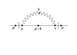
Figure 1: Feynman Diagram for the one-loop correction to the fermion self-energy.

The electron self-energy at one-loop order is shown in Fig. 1 and the regularized amplitude is given by

$$\displaystyle-i\Sigma(p)=\int\frac{d^{D}k}{(2\pi)^{D}}\Gamma^{\mu}S_{F}(p-k)\Gamma^{\nu}\Delta_{\mu\nu}(k),$$ (14)

where $\displaystyle D=d+1$. In what follows, all momentum integrations in the loop radiative quantities are computed using standard dimensional regularization procedure Bollini ; thooft , with $\displaystyle e\to\mu^{\epsilon/2}e$, $\displaystyle d=2-\epsilon$ and $\displaystyle\mu$ is the dimensional regularization energy scale.

By substituting the propagators and vertices in Eq. (14), we obtain

$$-i\Sigma(p)=\frac{(ie)^{2}\mu^{\epsilon}c}{2}\int\frac{d^{D}k}{(2\pi)^{D}}\dfrac{N_{1}}{D_{1}},$$ (15)

where $\displaystyle N_{1}$ and $\displaystyle D_{1}$ are given, respectively, by

$$\displaystyle N_{1} \displaystyle= \displaystyle v_{F}(p-k)_{i}\left(\gamma^{0}\gamma^{i}\gamma_{0}+\beta^{2}\gamma^{j}\gamma^{i}\gamma_{j}\right)$$ (16)

$$\displaystyle+ \displaystyle(p-k)_{0}\left(\gamma^{0}\gamma^{0}\gamma_{0}+\beta^{2}\gamma^{j}\gamma^{0}\gamma_{j}\right)$$

$$\displaystyle+ \displaystyle Mc^{2}\left(\gamma^{0}\gamma_{0}+\beta^{2}\gamma^{j}\gamma_{j}\right),$$

$$\displaystyle D_{1} \displaystyle= \displaystyle\left[(p-k)_{0}^{2}-v_{F}^{2}({\bf p}-{\bf k})^{2}-M^{2}c^{4}\right]$$ (17)

$$\displaystyle\times \displaystyle\sqrt{k_{0}^{2}-c^{2}\,{\bf k}^{2}-m^{2}c^{4}}.$$

Using, hereinafter, the gamma matrix properties $\displaystyle\gamma^{0}\gamma_{0}=1$ and $\displaystyle\gamma^{j}\gamma_{j}=2$, we have that

$$-i\Sigma(p)=\frac{(ie)^{2}\mu^{\epsilon}c}{2}\int\frac{dk_{0}}{2\pi}\frac{d^{d}k}{(2\pi)^{d}}\dfrac{\gamma^{0}(p-k)_{0}\left(1+2\beta^{2}\right)-v_{F}\gamma^{i}(p-k)_{i}+\left(1+2\beta^{2}\right)Mc^{2}}{[(p-k)_{0}^{2}-v_{F}^{2}({\mathbf{p}}-{\mathbf{k}})^{2}-M^{2}c^{4}](\sqrt{k_{0}^{2}-c^{2}\,{\mathbf{k}}^{2}-m^{2}c^{4}})}.$$ (18)

Using the Feynman parameterization,

$$\frac{1}{a\sqrt{b}}=\dfrac{3}{4}\int_{0}^{1}dx\left\{\frac{(1-x)^{-1/2}}{{[a\,x+(1-x)\,b]^{3/2}}}\right\},$$ (19)

and performing the integration in $\displaystyle k_{0}$, we obtain that Eq. (18) can be rewritten as

$$-i\Sigma(p)=\frac{(ie)^{2}\mu^{\epsilon}c}{4\pi}\int_{0}^{1}\dfrac{dx}{\sqrt{1-x}}\int\frac{d^{d}k}{(2\pi)^{d}}\dfrac{N_{2}}{D_{2}},$$ (20)

where $\displaystyle N_{2}$ and $\displaystyle D_{2}$ are defined, respectively, as

$$\displaystyle N_{2} \displaystyle= \displaystyle\left(1+2\beta^{2}\right)Mc^{2}+\left(1-2\beta^{2}\right)\gamma^{0}p_{0}(1-x)$$ (21)

$$\displaystyle- \displaystyle\left(1-{\frac{v^{2}_{F}x}{\cal B}}\right)v_{F}\gamma^{i}p_{i},$$

$$\displaystyle{D_{2}} \displaystyle= \displaystyle{\cal B}\left[\left({\bf k}-\frac{{\bf p}v^{2}_{F}x}{{\cal B}}\right)^{2}-{\frac{{\bf p}^{2}{{v_{F}}}^{4}{x}^{2}}{{\cal B}^{2}}}+{\frac{\cal A}{\cal B}}\right],$$ (22)

with $\displaystyle{\cal A}$ and $\displaystyle{\cal B}$ defined as

$$\displaystyle{\cal A} \displaystyle= \displaystyle p^{2}_{0}{x}^{2}+\left[({M}^{2}-m^{2}){c}^{4}+{\bf p}^{2}{{v_{F}}}^{2}-p^{2}_{0}\right]x+{m}^{2}{c}^{4},$$

$$\displaystyle{\cal B} \displaystyle= \displaystyle c^{2}\left[1-x\,(1-\beta^{2})\right].$$ (24)

The electron self-energy then becomes,

$$-i\Sigma(p)=\frac{(ie)^{2}\,c\mu^{\epsilon}}{4\pi}\int_{0}^{1}\dfrac{dx}{{\cal B}\sqrt{1-x}}\int\frac{d^{d}k}{(2\pi)^{d}}\dfrac{N_{2}}{k^{2}-\Delta},$$ (25)

where

$$\Delta={\frac{{\bf p}^{2}{{v_{F}}}^{4}{x}^{2}}{{\cal B}^{2}}}+{\frac{\cal A}{\cal B}}.$$ (26)

Performing the integration in the arbitrary dimension $\displaystyle d=2-\epsilon$ in Eq. (25) in the dimensional regularization procedure, we obtain

$$\displaystyle\Sigma(p) \displaystyle= \displaystyle\frac{(ie)^{2}\,c\mu^{\epsilon}}{16\pi^{2}}\int_{0}^{1}\dfrac{dx}{\sqrt{1-x}}\frac{\Gamma\left(\tfrac{\epsilon}{2}\right)\,N_{2}}{{\cal B}}\left[\dfrac{\Delta}{4\,\pi}\right]^{-\tfrac{\epsilon}{2}}$$ (27)

$$\displaystyle= \displaystyle\frac{(ie)^{2}\,c}{16\pi^{2}}\int_{0}^{1}\dfrac{dx}{\sqrt{1-x}}\frac{N_{2}}{{\cal B}}$$

$$\displaystyle\times \displaystyle\left[\frac{2}{\epsilon}-\gamma_{E}-\ln\left(\frac{\Delta}{4\pi\mu^{2}}\right)+{\cal O}(\epsilon)\right]$$

$$\displaystyle= \displaystyle\Sigma_{\rm finite}(p)+\Sigma_{\rm div}(p),$$

where

$$\displaystyle\Sigma_{\rm finite}(p) \displaystyle= \displaystyle-\frac{(ie)^{2}\,c}{16\pi^{2}}\int_{0}^{1}\dfrac{dx}{\sqrt{1-x}}\frac{N_{2}}{{\cal B}}$$ (28)

$$\displaystyle\times \displaystyle\left[\gamma_{E}+\ln\left(\frac{\Delta}{4\pi\mu^{2}}\right)\right]$$

and

$$\displaystyle\Sigma_{\rm div}(p)=\frac{(ie)^{2}\,c}{8\pi^{2}\epsilon}\int_{0}^{1}\dfrac{dx}{\sqrt{1-x}}\frac{N_{2}}{{\cal B}}$$ (29)

are the finite and divergent contributions to the electron self-energy, respectively, in the pseudo-Proca QED. One notices that the divergent part of the electron self-energy, Eq. (29), is independent of the vector field mass and it is in fact exactly the same result as that obtained in the PQED case livroMarino . Consequently, the Fermi velocity renormalization will also be the same.

Substituting Eq. (21) in Eq. (28), we immediately read the one-loop contributions to the electron mass and the wave-function renormalization terms. In particular, the one-loop correction for the fermion mass at zero-external momenta is

$$\displaystyle\Sigma_{\rm finite}^{M}(0)= \displaystyle\frac{e^{2}\,c}{16\pi^{2}}\left(1+2\beta^{2}\right)M\int_{0}^{1}\dfrac{dx}{\sqrt{1-x}}\,$$

$$\displaystyle\frac{1}{1-x\,(1-\beta^{2})} \displaystyle\left\{\gamma_{E}+\ln\left[\frac{M^{2}c^{2}x+m^{2}c^{2}(1-x)}{4\pi\mu^{2}[1-x\,(1-\beta^{2})]}\right]\right\}.$$

The PQED result is obtained by simply setting $\displaystyle m=0$ in Eq. (LABEL:SigmaM).

In Fig. 2 we show the behavior of the ratio $\displaystyle\Delta\Sigma^{M}\equiv[\Sigma_{\rm finite}^{M}(0)-\lim_{m\to 0}\Sigma_{\rm finite}^{M}(0)]/(Mc^{2})$ as a function of ($\displaystyle m/M$). We note that the electron self-energy correction increases with the vector field mass.

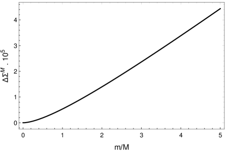
Figure 2: The difference of the self-energy correction for the fermion mass, with respect to the PQED one, as a function of the mass ratio ($\displaystyle m/M$). For illustrative purposes only, the Fermi velocity was taken to be $\displaystyle v_{F}=c/300$ and we also have used $\displaystyle e^{2}=4\pi v_{F}\alpha$, where $\displaystyle\alpha=1/137$ is the fine-structure constant.

III.2 The vector field self-energy

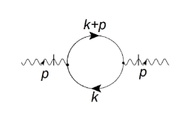
Figure 3: The one-loop vector field vacuum polarization diagram.

Let us now compute the vector field self-energy, shown in Fig. 3, for the present model. Explicitly, we have that

$$\displaystyle i\Pi^{\mu\nu}(p_{0},\textbf{p})=-\int\frac{d^{D}k}{(2\pi)^{D}}\texttt{Tr}\Big{[}\Gamma^{\mu}S_{F}(k+p)\Gamma^{\nu}S_{F}(k)\Big{]}.$$

(31)

The manipulation of the Dirac algebra proceeds in a standard fashion Peskin . Separating the components of the polarization tensor and performing the integration over $\displaystyle k_{0}$ and k in Eq. (31), we can write

$$\displaystyle\!\!\!\!\!\!\Pi^{00}(\bar{p})\!\! \displaystyle= \displaystyle\!\!\frac{e^{2}}{8\pi v_{F}}\left[I_{1}+\frac{(\bar{p}^{2}-2p_{0}^{2})I_{2}}{v_{F}}\right.\left.+\frac{Mc^{2}I_{3}}{v_{F}^{2}}\right],$$ (32)

$$\displaystyle\!\!\!\!\!\!\Pi^{ij}(\bar{p}) \displaystyle= \displaystyle\frac{e^{2}v_{F}}{8\pi c^{2}}\left[\left(\frac{\eta^{ij}\bar{p}^{2}}{v_{F}^{2}}-2p^{i}p^{j}\right)I_{2}\right.$$ (33)

$$\displaystyle+ \displaystyle\left.\eta^{ij}\left(I_{1}+\frac{Mc^{2}I_{3}}{v_{F}^{2}}\right)\right],$$

$$\displaystyle\!\!\!\!\!\!\Pi^{0j}(\bar{p}) \displaystyle= \displaystyle-\frac{e^{2}}{4\pi v_{F}c}p^{0}p^{j}I_{2},$$ (34)

where for convenience we have introduced the notation $\displaystyle\bar{p}=\sqrt{p^{2}_{0}-v^{2}_{F}{\bf p}^{2}}$ and $\displaystyle I_{1}$, $\displaystyle I_{2}$ and $\displaystyle I_{3}$ are given, respectively, by

$$\displaystyle I_{1} \displaystyle= \displaystyle\frac{1}{v_{F}}\int_{0}^{1}dx\sqrt{x(1-x)\bar{p}^{2}-M^{2}c^{4}}$$

$$\displaystyle= \displaystyle\frac{-i}{8v_{F}\bar{p}}\left\{4Mc^{2}\bar{p}+\left[4M^{2}c^{4}-\bar{p}^{2}\right]\ln{\left(\frac{2Mc^{2}+\bar{p}}{{2Mc^{2}-\bar{p}}}\right)}\right\},$$

$$\displaystyle I_{2} \displaystyle= \displaystyle v_{F}\int_{0}^{1}dx\frac{x(1-x)}{\sqrt{x(1-x)\bar{p}^{2}-M^{2}c^{4}}}$$

$$\displaystyle= \displaystyle\frac{i\,v_{F}}{8\bar{p}^{3}}\left\{4Mc^{2}\bar{p}+\left[4M^{2}c^{4}+\bar{p}^{2}\right]\ln{\left(\frac{2Mc^{2}+\bar{p}}{2Mc^{2}-\bar{p}}\right)}\right\},$$

$$\displaystyle I_{3} \displaystyle= \displaystyle\int_{0}^{1}\frac{v_{F}\ dx}{\sqrt{x(1-x)\bar{p}^{2}-M^{2}c^{4}}}=\frac{i\,v_{F}}{\bar{p}}\ln{\left(\frac{2Mc^{2}+\bar{p}}{2Mc^{2}-\bar{p}}\right)}.$$

Notice that the use of the dimensional regularization scheme makes the vector field self-energy explicitly finite. Furthermore, as at the one-loop level the vector field self-energy involves only the electron propagator, the result turns out to be identical to that computed in the context of the 2+1-D $\displaystyle QED$ at one-loop order.

III.3 Vertex correction and the g-factor

To have a complete one-loop analysis of relevant quantities, we also compute next the one-loop interaction vertex radiative contribution $\displaystyle\Gamma^{\nu}_{\rm 1L}$ as shown in Fig. 4.

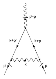
Figure 4: Feynman diagram for the one-loop correction to the interaction vertex.

Explicitly, $\displaystyle\Gamma^{\nu}_{\text{1}L}$ is given by

$$\Gamma^{\nu}_{\rm 1L}=\int\frac{d^{D}k}{(2\pi)^{D}}\Gamma^{\alpha}S_{F}(k+p^{\prime})\Gamma^{\nu}S_{F}(k+p)\Gamma^{\beta}\Delta_{\alpha\beta}(k).$$ (38)

We will analyze the quantity $\displaystyle M^{i}=\overline{u}(p^{\prime})\Gamma^{i}u(p)$, which relates to the two external fermion lines, $\displaystyle\bar{u}(p^{\prime})$ and $\displaystyle u(p)$, in the spatial component of the vertex diagram (because the temporal part of it does not affect the g-factor), such that we can use the Dirac equations to simplify the calculations further.

When represented according to the flux choices in Fig. 4, and after applying a parameterization detailed in the Appendix A, the diagram is written in its parameterized form as

$$M^{i}=\bar{u}(p^{\prime})\left(\int_{0}^{1}{dx}\int_{0}^{1-x}\dfrac{dy}{6\pi^{2}}\dfrac{M\,p^{i}v_{F}^{2}}{\sqrt{1-x-y}}\,\dfrac{N_{3}}{\cal K}\right)\,u(p),$$ (39)

with

$$N_{3}=\frac{2(1-x-y)\gamma^{j}\omega_{j}p_{i}v_{F}^{2}}{{\cal D}}-\frac{[\omega_{i}-2(x+y)^{2}p_{i}]\beta^{4}}{{\cal D}^{2}},$$ (40)

where $\displaystyle{\cal D}$ in the above equation is defined as

$${\cal D}=[(1-\beta^{2})\,(x+y)-1],$$ (41)

and

$$\displaystyle{\cal K} \displaystyle= \displaystyle{\cal D}^{2}\left(M^{2}c^{4}-m^{2}c^{4}-\omega_{0}^{2}\right)c^{2}+\left[v_{F}^{2}(p^{\prime}-p)_{i}^{2}+p_{0}^{2}\right]xy$$ (42)

$$\displaystyle+ \displaystyle\left[(x+y)(1-x-y)c^{2}\right](p^{\prime}+p)_{\mu}^{2}+p_{0}^{2}y^{2},$$

where $\displaystyle\omega_{0}=x\,p_{0}^{\prime}+y\,p_{0}$ and $\displaystyle\omega_{i}=x\,p^{\prime}+y\,p$. Then, we detach the terms proportional to $\displaystyle\sigma^{i\alpha}$ from Eq. (39) using Gordon decomposition to select the terms $\displaystyle M_{g}^{i}$ that are relevant to the g-factor (for more details, see App. A)

$$\displaystyle M^{i}_{g} \displaystyle= \displaystyle\bar{u}(p^{\prime})\left\{\int_{0}^{1}dx\int_{0}^{1-x}\frac{dy}{6\pi^{2}}\frac{\;M\,v_{F}\,\sigma^{i\alpha}(p^{\prime}-p)_{\alpha}\beta^{2}\textbf{}}{{\cal K}\sqrt{1-x-y}}\right.$$ (43)

$$\displaystyle\times \displaystyle\left.\left[{\dfrac{2(x+y)}{\cal D}}-{\dfrac{\beta^{2}(x+y)^{2}}{{\cal D}^{2}}}\right]\right\}u(p),$$

where the subscribed $\displaystyle g$ index was used to identify that we are only accounting for the $\displaystyle\sigma^{i\alpha}=(i/2)\left[\gamma_{\alpha},\gamma_{i}\right]$ terms which contribute to the gyromagnetic factor.

To extract the g-factor, however, a few conditions are also necessary, such as the low-energy approximation ($\displaystyle q^{2}\rightarrow{0}$) and the mass-shell condition (which for small energy values reads as $\displaystyle v_{F}\gamma^{j}p_{j}\cong Mc^{2}$) Peskin ; fator-g . After taking the above conditions, we conveniently define a variable

$$\displaystyle{\cal K^{\prime}} \displaystyle= \displaystyle\{[(x+y)^{2}-x-y]v_{F}^{2}-[(1-x-y)^{2}]c^{2}\}m^{2}c^{4}$$

$$\displaystyle+ \displaystyle 2\{[(x+y)^{2}-x-y]c^{2}-2(x+y)^{2}v_{F}^{2}\}M^{2}c^{4},$$

so that the relevant parts of the vertex correction $\displaystyle M_{g}^{i}$ are reduced to

$$\displaystyle M^{i}_{g} \displaystyle= \displaystyle\bar{u}(p^{\prime})\left\{\dfrac{1}{6\pi^{2}}\int_{0}^{1}dx\int_{0}^{1-x}dy\dfrac{\,M^{2}c^{2}\,\sigma^{i\alpha}q_{\alpha}v_{F}^{3}}{{\cal K^{\prime}}\sqrt{1-x-y}}\right.$$ (45)

$$\displaystyle\times \displaystyle\left.\left[{2\left(x+y\right){\cal D}-\left(x+y\right)^{2}v_{F}^{2}}\right]\right\}u(p).$$

We can also identify the g-factor correction form factor $\displaystyle F_{2}$ by comparing Eq. (43) to

$$M^{i}_{g}=i\,e\,\beta\,\bar{u}(p^{\prime})\left(\dfrac{i}{2Mc^{2}}\,F_{2}\,v_{F}\,\sigma^{i\nu}q_{\nu}\right)u(p).$$ (46)

Therefore, $\displaystyle F_{2}$ is turned into an integral related to the one obtained in Ref. fator-g , but in the present work a contribution depending on the effective vector field mass $\displaystyle m$ also appears. We then find

$$F_{2}=-i\dfrac{\alpha^{*}\,\beta^{3}}{2\pi}\,{R},$$ (47)

with $\displaystyle\alpha^{*}=e^{2}/4\pi v_{F}$ the effective fine-structure constant and

$$\displaystyle\displaystyle{R}={R}\left(\beta,\frac{m}{M}\right)=\int\displaylimits_{0}^{1}dx\int\displaylimits_{0}^{1-x}\frac{dy}{\sqrt{1-x-y}}$$

$$\displaystyle\frac{2(1+2\beta^{2})(x+y)+\beta^{2}(x+y)^{2}}{\frac{m^{2}}{M^{2}}(1-x-y){\cal D}^{2}-(x+y)^{2}{\cal D}}$$ (48)

a mass-dependent parametric integral.

A few predictions emerge from the result in Eq. (47) when looking at some of the limits achievable through the tweak of mass parameters: The mostly intuitive case occurs when the vector field is heavy with respect to the electron mass, $\displaystyle m\gg M$, which implies that the parametric integral assumes the form

$$\displaystyle\displaystyle{R}\Bigr{|}_{m\gg M}\simeq\frac{M^{2}}{m^{2}}\int\displaylimits_{0}^{1}dx\int\displaylimits_{0}^{1-x}\frac{dy(x+y)}{(1-x-y)^{3/2}}$$

$$\displaystyle\frac{2+4\beta^{2}+\beta^{2}(x+y)}{[(1-\beta^{2})\,(x+y)-1]^{2}}$$ (49)

and, consequently, $\displaystyle{F_{2}}=0$, i.e., the g-factor vanishes.

The second relevant limit happens when $\displaystyle m$ goes to zero in the original unprojected model, which after the projection reproduces the usual PQED behavior, i.e.,

$$\lim_{m\rightarrow 0}F_{2}=F_{2}^{\mathrm{PQED}}.$$ (50)

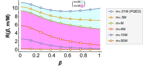
Figure 5: (Color Online). Dependence of $\displaystyle R$ on the ratio $\displaystyle m/M$ of the three-dimensional vector field mass to the electron mass. For $\displaystyle(m/M)=0$, the PQED results are retrieved and for $\displaystyle(m/M)\gg 1$ the g-factor is vanishingly small. The solid blue line (obtained near the limit of non-massive gauge field) is related to PQED and gives the approximate values of $\displaystyle R$ to correct the g-factor obtained in Ref. fator-g .

Figure 6: (Color Online). Dependence of $\displaystyle{R}$ on the ratio ($\displaystyle m/M$) for some values of $\displaystyle\beta$ obtained numerically. We notice that the vector field mass suppresses the result of the integral (and consequently of the $\displaystyle g$-factor) for all values of $\displaystyle\beta$, but does it faster for ultra-relativistic systems ($\displaystyle v_{F}\approx c$).

As a consistency check, we take the limit of Eq. (48) when $\displaystyle(m/M)\to 0$ and obtain

$$\displaystyle\displaystyle R=\int\displaylimits_{0}^{1}dx\int\displaylimits_{0}^{1-x}\frac{dy}{\sqrt{1-x-y}}\frac{2+4\beta^{2}+\beta^{2}(x+y)}{(x+y)[1-(1-\beta^{2})\,(x+y)]},$$ (51)

which has a similar structure to the parametric integral in Ref. fator-g , except that the term 2 in the numerator of Eq. (51) was missing in that reference. Hence, our result not only extends the projection to the massive case, but also corrects the g-factor result for graphene found previously in Ref. fator-g .

Although we could not find an analytical solution for the integral in Eq. (48), some numerical solutions for $\displaystyle R$ are shown in Fig. 5 for different mass ratios ($\displaystyle m/M$). These numerical values of $\displaystyle R$, when substituted into Eq. (47), allow us to verify how small changes in $\displaystyle\beta$ affect the g-factor in each case.

To show that the g-factor associated with the system is going to decrease faster with the mass when $\displaystyle v_{F}$ gets closer to $\displaystyle c$, we plot in Fig. 6 the numerical values of $\displaystyle{R}$ for a few different values of $\displaystyle\beta$, but now as a function of the mass ratio ($\displaystyle m/M$).

IV Conclusions

In this work, we have provided a generalization of the dimensional reduction, developed in Ref. Marino1 , for the case of a (3+1)D massive vector field. By doing so, we have obtained an effective planar model that retains the fundamental physical properties of the Proca electrodynamics, which is taken as an effective model for describing massive (via the Anderson-Higgs-Meissner mechanism) photons in a material. We have then evaluated the one-loop radiative corrections for the electron and vector field self-energies for this model.

We observed that the divergent part of the electron self-energy is exactly identical to the one obtained in the context of the PQED (massless) model. Therefore, from the renormalization group perspective, the renormalization of the Fermi velocity does not depend on the mass of the vector field and, consequently, it is identical to the one obtained for the PQED model Voz2 ; livroMarino , even though the effective mass for the electron is seen to increase with the vector field mass.

For the vertex diagram, we have found that the parametric integral in its form factor — and thus this theory’s predicted g-factor — decreases with both the value of $\displaystyle\beta$ and the ratio ($\displaystyle m/M$), effectively switching the magnetic coupling off of the system for very large values of $\displaystyle m$.

This work contributes to the proper description of planar effective models, which are known to be intrinsically related to condensed-matter physical systems, by investigating the effects of attributing a mass to the interaction field.

Appendix A Vertex correction

To shed more light on the g-factor corrections that come from the vertex developed in Subsec. III.3, we make the steps that differ from the usual QED more explicit. The subtlety on the calculation that appears for the model discussed here comes from the fact that it is anisotropic and has a different photon propagator (the planar projection of a massive vector field).

Starting from the vertex structure in Subsec. III.3,

$$\Gamma^{\nu}_{\rm 1L}=\int\frac{d^{D}k}{(2\pi)^{D}}\Gamma^{\alpha}\underbrace{S_{F}(k+p^{\prime})\Gamma^{\nu}S_{F}(k+p)}_{\rho^{\nu}}\Gamma^{\beta}\Delta_{\alpha\beta}(k),$$ (52)

we define an auxiliary variable $\displaystyle\rho^{\nu}$ and expand the indices $\displaystyle\alpha$ and $\displaystyle\beta$ to get

$$\Gamma^{\nu}_{\rm 1L}=\int\frac{d^{D}k}{(2\pi)^{D}}\left[\Gamma^{0}{\rho^{\nu}}\Gamma^{0}\Delta_{00}(k)+\Gamma^{l}{\rho^{\nu}}\Gamma^{n}\Delta_{ln}(k)\right].$$ (53)

In Eq. (53), the non-diagonal terms of the vector field propagator were dropped because the metrics inside them vanish. Explicitly substituting the Feynman rules given in Sec. III, we find

$$\displaystyle\Gamma^{\nu}_{\rm 1L}=-\frac{ie^{2}c}{2}\mu\displaystyle\int\frac{d^{D}k}{(2\pi)^{D}}$$

$$\displaystyle\left\{\gamma^{0}\left(\dfrac{\gamma^{0}(k+p^{\prime})_{0}+v_{F}\gamma^{i}(k+p^{\prime})_{i}+Mc^{2}}{(k+p^{\prime})_{0}^{2}-v_{F}^{2}{\bf(k+p^{\prime})}^{2}-M^{2}c^{4}}\right)\right.\Gamma^{\nu}\left(\dfrac{\gamma^{0}(k+p)_{0}+v_{F}\gamma^{i}(k+p)_{i}+Mc^{2}}{(k+p)_{0}^{2}-v_{F}^{2}{\bf(k+p)}^{2}-M^{2}c^{4}}\right)\gamma^{0}\left[\frac{1}{\sqrt{k_{0}^{2}-c^{2}\,{\mathbf{k}}^{2}-m^{2}c^{4}}}\right]+$$

$$\displaystyle\beta^{2}\gamma^{l}{\left(\dfrac{\gamma^{0}(k+p^{\prime})_{0}+v_{F}\gamma^{i}(k+p^{\prime})_{i}+Mc^{2}}{(k+p^{\prime})_{0}^{2}-v_{F}^{2}{\bf(k+p^{\prime})}^{2}-M^{2}c^{4}}\right)}{\Gamma^{\nu}\left(\dfrac{\gamma^{0}(k+p)_{0}+v_{F}\gamma^{i}(k+p)_{i}+Mc^{2}}{(k+p)_{0}^{2}-v_{F}^{2}{\bf(k+p)}^{2}-M^{2}c^{4}}\right)}\left.\gamma^{n}\left[\frac{\eta_{ln}}{\sqrt{k_{0}^{2}-c^{2}\,{\mathbf{k}}^{2}-m^{2}c^{4}}}\right]\right\}.$$ (54)

To handle this unusual photon propagator, which contains a square root and a mass term, we apply a slightly modified Feynman parameterization,

$$\frac{1}{abd^{{1}/{2}}}=\frac{3}{4}\int_{0}^{1}dx\int_{0}^{1-x}dy\frac{(1-x-y)^{-{1}/{2}}}{[ax+by+d(1-x-y)]^{{5}/{2}}}$$ (55)

on the denominator of each term in Eq. (54). Assuming

$$\displaystyle a \displaystyle= \displaystyle{(k+p^{\prime})_{0}^{2}-v_{F}^{2}{\bf(k+p^{\prime})}^{2}-M^{2}c^{4}},$$

$$\displaystyle b \displaystyle= \displaystyle{(k+p)_{0}^{2}-v_{F}^{2}{\bf(k+p)}^{2}-M^{2}c^{4}},$$

$$\displaystyle d \displaystyle= \displaystyle 3{{k_{0}^{2}-c^{2}\,{\mathbf{k}}^{2}-m^{2}c^{4}}},$$

we find that the denominator of Eq. (54) is given by

$$\displaystyle\frac{1}{abc^{1/2}}=\frac{3}{4}\int_{0}^{1}dx\int_{0}^{1-x}dy\ (1-x-y)^{-1/2}$$

$$\displaystyle\{k_{0}^{2}(1+x+y)+[2k_{0}p_{0}^{\prime}+{p^{\prime}_{0}}^{2}]x$$

$$\displaystyle[{2k_{0}p_{0}+p_{0}^{2}-v_{F}^{2}{\mathbf{(}k+p)}^{2}-M^{2}c^{4}}]y+$$

$$\displaystyle-c^{2}\,{\mathbf{k}}^{2}-m^{2}c^{4}(1-x-y)\}^{-5/2}.$$

Now, we complete the $\displaystyle k_{0}$ square, make a shift $\displaystyle k_{0}\to k_{0}-\omega_{0}$ (with $\displaystyle\omega_{0}=x\,p_{0}^{\prime}+y\,p_{0}$) on it, and solve the integration over $\displaystyle k_{0}$ as done in standard anisotropic procedures (at this point, we also drop the odd terms in $\displaystyle k_{0}$).

Then, we follow essentially the same steps for $\displaystyle\mathbf{k}$, but using the shift $\displaystyle\mathbf{k}\to\mathbf{k}-\text{ \boldmath$\displaystyle\omega$}{\beta^{2}}/{\cal D}^{2}$, with $\displaystyle{\cal D}=[(1-\beta^{2})\,(x+y)-1]$ and $\displaystyle\text{ \boldmath$\displaystyle\omega$}=x\,\mathbf{p^{\prime}}+y\,\mathbf{p}$. Finally, we perform the integration over $\displaystyle\mathbf{k}$ using dimensional regularization Peskin to obtain Eq. (39), namely:

$$\Gamma^{i}_{\rm 1L}=\int_{0}^{1}{dx}\int_{0}^{1-x}\dfrac{dy}{6\pi^{2}}\left[\dfrac{N_{3}}{\cal K}\right]\dfrac{M\,p^{i}v_{F}^{2}}{\sqrt{1-x-y}},$$ (56)

where, for convenience, we defined the numerator result for the integration in $\displaystyle\mathbf{k}$ as

$$\displaystyle N_{3}=\left.\frac{2(1-x-y)\gamma^{j}\omega_{j}p_{i}v_{F}^{2}}{{\cal D}}\right.-\left.\frac{[\omega_{i}-2(x+y)^{2}p_{i}]\beta^{4}}{{\cal D}^{2}}\right.,$$

$$\displaystyle{\cal D}=[(1-\beta^{2})\,(x+y)-1],$$

and its denominator as

$$\displaystyle{\cal K}={\cal D}^{2}\left(M^{2}c^{4}-m^{2}c^{4}-\omega_{0}^{2}\right)c^{2}+\left[v_{F}^{2}(p^{\prime}-p)_{i}^{2}+p_{0}^{2}\right]xy$$

$$\displaystyle+\left[(x+y)(1-x-y)c^{2}\right](p^{\prime}+p)_{\mu}^{2}+p_{0}^{2}y^{2}.$$

Using the (Gordon) decomposition identity

$$\bar{u}(p^{\prime})\gamma^{\mu}u(p)=\bar{u}(p^{\prime})\left[\frac{(p^{\prime}+p)^{\mu}}{2Mc^{2}}+i\sigma^{\nu\mu}\frac{q_{\nu}}{2Mc^{2}}\right]\,u(p),$$

where $\displaystyle\bar{u}(p^{\prime})$ and $\displaystyle u(p)$ are spinorial solutions to the Dirac equations, $\displaystyle q_{\nu}$ is the transferred momentum given by $\displaystyle q_{\nu}=(p^{\prime}-p)_{\nu}$, and $\displaystyle\sigma_{\nu\mu}$ is defined as $\displaystyle\sigma_{\nu\mu}=(i/2)\left[\gamma_{\mu},\gamma_{\nu}\right]$, we stablish which of the terms of $\displaystyle M^{i}$ will be relevant to the g-factor. In other words, we select only the terms proportional to $\displaystyle\sigma^{i\alpha}$ from Eq. (39) and leave aside the terms that would have a $\displaystyle(p^{\prime}+p)^{\mu}$ to define

$$\begin{split}M^{i}_{g}=\bar{u}(p^{\prime})\left\{\int_{0}^{1}dx\int_{0}^{1-x}\frac{dy}{6\pi^{2}}\frac{\;M\,v_{F}\,\sigma^{i\alpha}(p^{\prime}-p)_{\alpha}\beta^{2}\textbf{}}{{\cal K}\sqrt{1-x-y}}\right.\\ \left.\left[{\dfrac{2(x+y)}{\cal D}}-{\dfrac{\beta^{2}(x+y)^{2}}{{\cal D}^{2}}}\right]\right\}u(p),\end{split}$$

as it appears in Eq. (43)

References

- (1) T. Ando, Y. Matsumoto, Y. Uemura, Theory of Hall Effect in a Two-Dimensional Electron System, Journ. of the Phys. Soc. of Japan 39, 279 (1975).
- (2) D.C. Tsui, H.L. Stormer, A.C. Gossard, Two-Dimensional Magnetotransport in the Extreme Quantum Limit, Phys. Rev. Lett. 48, 1559 (1982).
- (3) R.B. Laughlin, Anomalous Quantum Hall Effect: An Incompressible Quantum Fluid with Fractionally Charged Excitations, Phys. Rev. Lett. 50, 1395 (1983).
- (4) C.C. Chamon, E. Fradkin, Distinct universal conductances in tunneling to quantum Hall states: The role of contacts, Phys. Rev. B 56, 2012 (1997).
- (5) O. Heinonen, Composite Fermions: A Unified View of the Quantum Hall Regime, World Scientific Pub Co Inc (1998), and articles therein.
- (6) E.V. Gorbar, V.P. Gusynin, V.A. Miransky, I.A. Shovkovy, Coulomb interaction and magnetic catalysis in the quantum Hall effect in graphene, Physica Scripta T146, 014018 (2012).
- (7) I.F. Herbut, Interactions and Phase Transitions on Graphene’s Honeycomb Lattice, Phys. Rev. Lett. 97, 146401 (2006).
- (8) V.P. Gusynin, V.A. Miransky, S.G. Sharapov, I.A. Shovkovy, Excitonic gap, phase transition, and quantum Hall effect in graphene, Phys. Rev. B 74, 195429 (2006).
- (9) I.F. Herbut, V. Juricic, O. Vafek, Coulomb Interaction, Ripples, and the Minimal Conductivity of Graphene, Phys. Rev. Lett. 100, 046403 (2008).
- (10) V. Juricic, I.F. Herbut, G.W. Semenoff Coulomb interaction at the metal-insulator critical point in graphene, Phys. Rev. B 80, 081405(R) (2009).
- (11) M.A.H. Vozmediano, M. I. Katsnelson, F. Guinea, Gauge fields in graphene, Physics Reports 496, 109 (2010).
- (12) M.A.H. Vozmediano, F. Guinea, Effect of Coulomb interactions on the physical observables of graphene, Physica Scripta T146, 014015 (2011).
- (13) E.C. Marino, L.O. Nascimento, V.S. Alves, C.M. Smith, Interaction Induced Quantum Valley Hall Effect in Graphene, Phys. Rev. X 5, 011040 (2015).
- (14) N. Menezes, V.S. Alves, C.M. Smith The influence of a weak magnetic field in the Renormalization-Group functions of (2 + 1)-dimensional Dirac systems, Eur. Phys. J. B 89, 271 (2016).
- (15) W. Choi, N. Choudhary, G. H. Han, J. Park, D. Akinwande, Y.H. Lee, Recent development of two-dimensional transition metal dichalcogenides and their applications, Materials Today, Volume 20, 116 (2017).
- (16) E.C. Marino, L.O. Nascimento, V.S. Alves, N. Menezes, C.M. Smith, Quantum-electrodynamical approach to the exciton spectrum in transition-metal dichalcogenides, 2D Materials 5, 041006 (2018).
- (17) A.J. Chaves, R.M. Ribeiro, T. Frederico and N.M. R. Peres, Excitonic effects in the optical properties of 2D materials: an equation of motion approach, 2D Materials 4, 025086 (2017).
- (18) Z. Tesanovic, L. Xing, L. Bulaevskii, Q. Li, M. Suenaga Critical Fluctuations in the Thermodynamics of Quasi-Two-Dimensional Type-II Superconductors, Phys. Rev. Lett. 69, 3563 (1992).
- (19) S.-C. Zhang, SO(5) Quantum Nonlinear sigma Model Theory of the High Tc Superconductivity, Science 275, 1089 (1997).
- (20) M. Franz, Z. Tesanovic, O. Vafek, QED3 theory of pairing pseudogap in cuprates: From d-wave superconductor to antiferromagnet via an algebraic Fermi liquid, Phys. Rev. B 66, 054535 (2002).
- (21) S.A. Kivelson, I.P. Bindloss, E. Fradkin, V. Oganesyan, J.M. Tranquada, A. Kapitulnik,C. Howald, Distinct universal conductances in tunneling to quantum Hall states: The role of contacts, Rev. of Mod Phys. 75, 2012 (2003).
- (22) E.C. Marino, D. Niemeyer, V.S. Alves, T. Hansson, S. Moroz, Screening and topological order in thin superconducting films, New J. Phys. 20, 083049 (2018).
- (23) A.H. Castro Neto, F. Guinea, N.M.R. Peres, K.S. Novoselov, A.K. Geim, The electronic properties of graphene, Rev. Mod. Phys. 81, 109 (2009).
- (24) E.C. Marino, Quantum electrodynamics of particles on a plane and the Chern-Simons theory, Nucl. Phys. B 408, 551 (1993).
- (25) E.V. Gorbar, V.P. Gusynin, and V.A. Miransky, Dynamical chiral symmetry breaking on a brane in reduced QED, Phys. Rev. D 64, 105028 (2001).
- (26) S. Teber, Electromagnetic current correlations in reduced quantum electrodynamics, Phys. Rev. D 86, 025005 (2012).
- (27) A.V. Kotikov, S. Teber, Two-loop fermion self-energy in reduced quantum electrodynamics and application to the ultrarelativistic limit of graphene, Phys. Rev. D 89, 065038 (2014).
- (28) E.C. Marino, L.O. Nascimento, V.S. Alves, C.M. Smith, Unitarity of theories containing fractional powers of the d’Alembertian operator, Phys. Rev. D 90, 105003 (2014).
- (29) R.L.P.G. do Amaral and E.C. Marino, Canonical quantization of theories containing fractional powers of the d’Alembertian operator, J. of Physics : Mathematical and General 25, 5183 (1992).
- (30) L. Fernández, V.S. Alves, L.O. Nascimento,F. Peña, M. Gomes and E. C. Marino, Renormalization of the band gap in 2D materials through the competition between electromagnetic and four-fermion interactions, arXiv:2002.10027 [hep-th] (2020).
- (31) J.D. Silva, A.N. Braga, W.P. Pires, V.S. Alves, D.T. Alves, E.C.Marino, Inhibition of the Fermi velocity renormalization in a graphene sheet by the presence of a conducting plate, Nuclear Physics B 920, 221 (2017).
- (32) W.P. Pires, J.D. Silva, A.N. Braga, V.S. Alves, D.T. Alves, E.C. Marino, Cavity effects on the Fermi velocity renormalization in a graphene sheet, Nuclear Physics B 932, 529 (2018).
- (33) N. Menezes, V.S. Alves, E.C. Marino, L. Nascimento, L.O. Nascimento, C.M. Smith, Spin g-factor due to electronic interactions in graphene, Phys. Rev. B 95, 245138 (2016).
- (34) V.S. Alves, W.S. Elias, L.O. Nascimento, V. Juričić, F. Peña, Chiral symmetry breaking in the pseudo-quantum electrodynamics, Phys. Rev. D 87, 125002 (2013).
- (35) V.S. Alves, E.C. Marino, L.O. Nascimento, J.F. Medeiros Neto, R.F. Ozela and R.O. Ramos, Bounded particle interactions driven by a nonlocal dual Chern-Simons model, Physics Letters B 797, 134860 (2019).
- (36) Y. Cao, V. Fatemi, S. Fang, K. Watanabe, T. Taniguchi, E. Kaxiras, P. Jarillo-Herrero, Unconventional superconductivity in magic-angle graphene superlattices. Nature 556, 43 (2018)
- (37) E.F. Talantsev, R.C. Mataira, W.P. Crump, Classifying superconductivity in magic angle twisted bilayer graphene, Scientific Reports 10, 212 (2020).
- (38) V.S. Alves, T. Macrì, G.C. Magalhães, E.C. Marino, L.O. Nascimento, Two-dimensional Yukawa interactions from nonlocal Proca quantum electrodynamics, Phys. Rev. D 97, 096003 (2018).
- (39) M.E. Peskin and D.V. Schroeder, An Introduction to Quantum Field Theory, Perseus Books Publishing, New York, (1995); M.O.C. Gomes, Teoria Quântica dos Campos, Edusp (2002) (in Portuguese).
- (40) C. Bollini, J.J. Giambiagi, Dimensional Renormalization: The Number of Dimensions as a Regularizing Parameter, Il Nuovo Cimento B, 12, 20 (1972).
- (41) G. ’t Hooft, M. Veltman, Regularization and renormalization of gauge fields, Nuclear Physics B 44, 189 (1972).
- (42) E.C. Marino, Quantum Field Theory Approach to Condensed Matter Physics, Cambridge University Press (2017).
- (43) W. Sheng, A. Babinski, Zero g-factors and nonzero orbital momenta in self-assembled quantum dots, Phys. Rev. B 75, 033316 (2007).
- (44) R. Bi, Z. Feng, X. Li, J. Niu, J. Wang, Y. Shi, D. Yu, X. Wu, Spin zero and large Landé g-factor in , New Journal of Physics 20, 063026 (2018).
- (45) A. Giorgioni, S. Paleari, S. Cecchi, E. Vitiello, E. Grilli, G. Isella, W. Jantsch, M. Fanciulli, F. Pezzoli, Giant g-factor tuning of long-lived electron spins in Ge, Nature Communications 7, 13886 (2016).
- (46) B. Nedniyom, R.J. Nicholas, M.T. Emeny, L. Buckle, A.M. Gilbertson, P.D. Buckle, T. Ashley, Giant enhanced g-factors in an InSb two-dimensional gas, Phys. Rev. B 80, 125328, (2009).