1 Introduction

In recent years, the machine learning and statistics communities have witnessed a surge of interest in the Langevin diffusion process, and its connections to stochastic algorithms for sampling and optimization. The Langevin diffusion in ^d is defined via the Itô stochastic differential equation (SDE)

$$dX_{t}=b(X_{t})dt+dB_{t},$$ (1)

where $B_{t}$ is a standard $d$-dimensional Brownian motion, and the function $b:{}^{d}\to{}^{d}$ is known as the drift term. For a drift term of the form $b(x)=-\frac{1}{2}\nabla U(x)$ for some differentiable function $U:{}^{d}\rightarrow\real$, the Langevin process (1) has stationary distribution with density $\gamma(x)\propto e^{-U(x)}$; moreover, under mild growth conditions on $U$, the diffusion converges to this stationary distribution as $t\rightarrow\infty$. See Pavliotis (2014) for more background on these facts, which underlie the development of sampling algorithms based on discretizations of the Langevin diffusion. Diffusive processes of this nature also play an important role in understanding stochastic optimization; in this context, the Gaussian noise helps escaping shallow local minima and saddle points in finite time, making it especially useful for non-convex optimization. From a theoretical point of view, the continuous-time process is attractive to analyze, amenable to a range of tools coming from stochastic calculus and Brownian motion theory (Revuz and Yor, 1999). However, in practice, an algorithm can only run in discrete time, so that the understanding of discretized versions of the Langevin diffusion is very important.

The discretization of SDEs is a central topic in the field of scientific computation, with a wide variety of schemes proposed and studied (Kloeden, 1992; Higham, 2001). The most commonly used discretization is the Euler-Maruyama discretization: parameterized by a step size $\eta>0$, it is defined by the recursion

$$\hat{X}_{(k+1)\eta}=\hat{X}_{k\eta}+\eta b(\hat{X}_{k\eta})+\sqrt{\eta}\xi_{k},\quad\mbox{for $k=0,1,2,\ldots$.}$$ (2)

Here the sequence $\{\xi_{k}\}_{k=1}^{+\infty}$ is formed of $\mathrm{i.i.d.}$ $d$-dimensional standard Gaussian random vectors.

From past work, the Euler-Murayama scheme is known to have first-order accuracy under appropriate smoothness conditions. In particular, the Wasserstein distances $\mathcal{W}_{p}$ for $p\geq 1$ between the original Langevin diffusion and the discretized version decays as $O(\eta)$ as $\eta$ decays to zero, with the dimension $d$ and time horizon $T$ captured in the order notation (see, e.g., Alfonsi et al., 2015). When the underlying dependence on the time horizon $T$ is explicitly calculated, it can grow exponentially, due to the underlying Grönwall inequality. If the potential $U$ is both suitably smooth and strongly convex, then the scaling with $\eta$ remains first-order, and the bound becomes independent of time $T$ (Durmus and Moulines, 2017; Dalalyan and Karagulyan, 2017). These bounds, in conjunction with the coupling method, have been used to bound the mixing time of the unadjusted Langevin algorithm (ULA) for sampling from strongly-log-concave densities. Moreover, this bound aligns well with the classical theory of discretization for ordinary differential equations (ODEs), where finite-time discretization error may suffer from bad dependence on $T$, and either contraction assumptions or symplectic structures are needed in order to control long-time behavior (Iserles, 2009).

On the surface, it might seem that SDEs pose greater numerical challenges than ODEs; however, the presence of randomness actually has been shown to help in the long-term behavior of discretization. Dalalyan (2017) showed that the pathwise Kullback-Leibler (KL) divergence between the original Langevin diffusion (1) and the Euler-Maruyma discretization (2) is bounded as $O(\eta T)$ with only smoothness conditions. This result enables comparison of the discretization with the original diffusion over long time intervals, even without contraction. The discretization techniques of Dalalyan (2017) serve as a foundation for a number of recent papers on sampling and non-convex learning, including the papers (Raginsky et al., 2017; Tzen et al., 2018; Liang and Su, 2017).

On the other hand, this $O(\eta)$ bound on the KL error is likely to be loose in general. Under suitable smoothness conditions, standard transportation inequalities (Bolley and Villani, 2005) guarantee that such a KL bound can be translated into a $O(\sqrt{\eta})$-bound in Wasserstein distance. Yet, as mentioned in the previous paragraph, the Wasserstein rate should be $O(\eta)$ under enough smoothness assumption. This latter result either requires assuming contraction or leads to exponential time dependence, leading naturally to the question: can we achieve best of both worlds? That is, is it possible to prove a $O(\eta T)$ Wasserstein bound without convexity or other contractivity conditions?

Our contributions:

In this paper, we answer the preceding question in the affirmative: more precisely, we close the gap between the correct rate for the Euler-Maruyama method and the linear dependence on time horizon, without any contractivity assumptions. As long as the drift term satisfies certain first and second-order smoothness, as well as growth conditions at far distance, we show the KL divergence between marginal distributions of equation (1) and equation (2), at any time $T$, is bounded as $O(\eta^{2}d^{2}T)$. Note that this bound is non-asymptotic, with polynomial dependence on all the smoothness parameters, and linear dependence on $T$. As a corollary of this improved discretization bound, we give improved bounds for using the unadjusted Langevin algorithm (ULA) for sampling from a distribution satisfying a log-Sobolev inequality. In addition, our improved discretization bound improves a number of previous results on non-convex optimization and inference, all of which are based on the discretized Langevin diffusion.

In the proof of our main theorem, we introduce a number of new techniques. A central challenge is how to study the evolution of time marginals of the interpolation of discrete-time Euler algorithm, and in order to do so, we derive a Fokker-Planck equation for the interpolated process, where the drift term is the backward conditional expectation of $b$ at the previous step, conditioned on the current value of $x$. The difference between this new drift term for the interpolated process and $b$ itself can be much smaller than the difference between $b$ at two time points. Indeed, taking the conditional expectation cancels out the bulk of the noise terms, assuming the density from the previous step is smooth enough. We capture the smoothness of density at the previous step by its Fisher information, and develop De Bruijn-type inequalities to control the Fisher information along the path. Combining this regularity estimate with suitable tail bounds leads to our main result. We suspect that our analysis of this interpolated process and associated techniques for regularity estimates may be of independent interest.

Paper	Requirecontraction	Time $T$	Step size $\eta$	Requiremixing	Additionalassumptions
Dalalyan (2017)	No	$O(\sqrt{T})$	$O(\sqrt{\eta})$	No	None
Alfonsi et al. (2015)	No	$O(e^{cT})$	$O(\eta)$	No	Second-ordersmooth drift
Dalalyan and Karagulyan (2017),Durmus and Moulines (2017)	Yes	-	$O(\eta)$	Yes	Second-ordersmooth drift
Cheng and Bartlett (2018),Ma et al. (2018)	No	-	$O(\sqrt{\eta})$	Yes	strong convexityoutside a ball
Cheng et al. (2018a),Bou-Rabee et al. (2018)	No	-	$O(\eta)$	Yes	strong convexityoutside a ball
This paper	No	$O(\sqrt{T})$	$O(\eta)$	No	Second-ordersmooth drift

Table 1: Comparison between discretization of Langevin diffusion and sampling algorithms.

Related work:

Recent years have witnessed a flurry of activity in statistics and machine learning on the Langevin diffusion and related stochastic processes. A standard application is sampling from a density of the form $\gamma(x)\propto e^{-U(x)}$ based on an oracle that returns the pair $(U(x),\nabla U(x))$ for any query point $x$. In the log-concave case, algorithms for sampling under this model are relatively well-understood, with various methods for discretization and variants of Langevin diffusion proposed in order to refine the dependence on dimension, accuracy level and condition number (Dalalyan, 2017; Durmus and Moulines, 2017; Cheng et al., 2018b; Lee et al., 2018b; Mangoubi and Vishnoi, 2018; Dwivedi et al., 2018).

When the potential function $U$ is non-convex, the analysis of continuous-time convergence and the discretization error analysis both become much more involved. When the potential satisfies a logarithmic Sobolev inequalities, continuous-time convergence rates can be established (see e.g. Markowich and Villani, 2000), and these guarantees have been leveraged for sampling algorithms (Bernton, 2018; Wibisono, 2018; Ma et al., 2018). Coupling-based results for the Wasserstein distance $\mathcal{W}_{2}$ have also been shown for variants of Langevin diffusion (Cheng et al., 2018a; Bou-Rabee et al., 2018). Beyond sampling, the global convergence nature of Langevin diffusion has been used in non-convex optimization, since the stationary distribution is concentrated around global minima. Langevin-based optimization algorithms have been studied under log-Sobolev inequalities (Raginsky et al., 2017), bounds on the Stein factor (Erdogdu et al., 2018); in addition, accelerated methods have been studied (Chen et al., 2019). The dynamics of Langevin algorithms have also been studied without convergence to stationarity, including exiting times (Tzen et al., 2018), hitting times (Zhang et al., 2017), exploration of a basin-of-attraction (Lee et al., 2018a), and statistical inference using the path (Liang and Su, 2017). Most of the works in non-convex setting are based on the discretization methods introduced by Dalalyan (2017).

Finally, in a concurrent and independent line of work, Fang and Giles (2019) also studied a multi-level sampling algorithm without imposing a contraction condition, and obtained bounds for the mean-squared error; however, their results do not give explicit dependence on problem parameters. Since the proofs involve bounding the moments of Radon-Nikodym derivative, their results may be exponential in dimension, as opposed to the polynomial-dependence given here.

Notation:

We let $\|x\|_{2}$ denote the Euclidean norm of a vector $x\in{}^{d}$. For a matrix $M$ we let $|\!|\!|M|\!|\!|_{{\tiny{\mbox{op}}}}$ denote its spectral norm. For a function $b:{}^{d}\rightarrow{}^{d}$, we let $\nabla b(x)\in{}^{d\times d}$ denote its Jacobian evaluated at $x$. We use $\mathcal{L}(X)$ to denote the law of random variable $X$. We define the constant $A_{0}=\|b(0)\|_{2}$. When the variable of the integrand is not explicitly written, integrals are taking with respect to the Lebesgue measure: in particular, for an integrable function $g:{}^{d}\rightarrow\real$, we use $\int g$ as a shorthand for $\int_{{}^{d}}g(x)dx$. For a probability density function $p$ (with respect to the Lebesgue measure) in ^d, we let $H(p)$ to denote the differential entropy of $p$.

2 Main Results

We now turn to our main results, beginning with our assumptions and a statement of our main theorem. We then develop and discuss a number of corollaries of these main results.

2.1 Statement of main results

Our main results involve three conditions on the drift term $b$, and one on the initialization:

Assumption 1 (Lipschitz drift term).

There is a finite constant $L_{1}$ such that

$$\|b(x)-b(y)\|_{2}\leq L_{1}\|x-y\|_{2}\quad\mbox{for all $x,y\in{}^{d}$.}$$ (3)

Assumption 2 (Smooth drift term).

There is a finite constant $L_{2}$ such that

$$|\!|\!|\nabla b(x)-\nabla b(y)|\!|\!|_{{\tiny{\mbox{op}}}}\leq L_{2}\|x-y\|_{2}\quad\mbox{for all $x,y\in{}^{d}$.}$$ (4)

Assumption 3 (Distant dissipativity).

There exist strictly positive constants $\mu,\beta$ such that

$$\langle b(x),x\rangle\leq-\mu\|x\|_{2}^{2}+\beta\quad\mbox{for all $x\in{}^{d}$.}$$ (5)

Assumption 4 (Smooth Initialization).

The initializations $X_{0}$ and $\hat{X}_{0}$, for the processes (1) and (2) respectively, are drawn from a density $\pi_{0}$ such that

$$-\log\pi_{0}(x)\leq h_{0}+\frac{\|x\|_{2}^{2}}{\sigma_{0}^{2}}\quad\mbox{for all $x\in{}^{d}$.}$$ (6)

Note that no contractivity assumption on the drift term $b$ is imposed. Rather, we use the notion of distant dissipativity, which is substantially weaker; even this assumption is relaxed in Theorem 2. The initialization condition (6) is clearly satisfied by the standard Gaussian density, but Assumption 4 allows for other densities with quadratic tail behavior.

With these definitions, the main result of this paper is the following:

Theorem 1.

Consider the original Langevin diffusion (1) under Assumptions 1,  2,  3 and 4. Then there are universal constants $(c_{0},c_{1})$ such that for any $\eta\in(0,\frac{1}{2L_{1}})$ and all times $T>0$, the KL error of the Euler-Maruyama discretization (2) is bounded as

$$D_{\text{KL}}(\hat{\pi}_{T}\|\pi_{T})\leq c_{0}\eta^{2}\bigg{(}h_{0}+H(\pi_{0})+A_{0}^{2}+\Big{(}\sigma_{0}^{2}d+\frac{\beta+d}{\mu}\Big{)}\Big{(}\frac{1}{\sigma_{0}^{2}}+TL_{1}^{2}\Big{)}+TL_{2}^{2}d^{2}\bigg{)}\\ +c_{1}\eta^{4}L_{2}^{2}\bigg{(}A_{0}^{4}+L_{1}^{4}\Big{(}\sigma_{0}^{2}d+\frac{(\beta+d)^{2}}{\mu}+d^{2}\Big{)}\bigg{)}.$$ (7)

If we track only the dependence on $(\eta,T,d)$, the result (7) can be summarized as a bound of the form $D_{\text{KL}}(\hat{\pi}_{T}\|\pi_{T})\lesssim\eta^{2}d^{2}T$. This result should be compared to the $O(\eta dT)$ bound obtained by Dalalyan (2017) using only Assumption 2. It is also worth noticing that the term $\eta^{2}d^{2}L_{2}^{2}T$ only comes with the third order derivative bound, which coincides with the Wasserstein distance result, based on a coupling proof, as obtained by Durmus and Moulines (2017) and Dalalyan and Karagulyan (2017). However, these works do not study separately the discretization error of the discrete process and assume contractivity.

Note that Assumption 3 can be substantially relaxed when the drift is negative gradient of a function. Essentially, we only require this function to be non-negative, along with the smoothness assumptions. In such case, we have the following discretization error bound:

Theorem 2.

Consider the original Langevin diffusion (1) under Assumptions 1,  2, and 4, and suppose that $b=-\nabla f$ for some non-negative function $f$. Then for any stepsize $\eta\in(0,\frac{1}{2L_{1}})$ and time $T>0$, the KL error of the Euler-Maruyama discretization (2) is bounded as

$$D_{\text{KL}}(\hat{\pi}_{T}\|\pi_{T})\leq c_{0}\eta^{2}\bigg{(}A_{0}^{2}+\Big{(}\sigma_{0}^{2}d+f(0)+L_{1}T\sigma_{0}^{2}(h_{0}+H(\pi_{0})+d)\Big{)}\Big{(}\frac{1}{\sigma_{0}^{2}}+TL_{1}^{2}\Big{)}+TL_{2}^{2}d^{2}\bigg{)}\\ +c_{1}\eta^{4}L_{2}^{2}\bigg{(}A_{0}^{4}+L_{1}^{4}\Big{(}f(0)^{2}+L_{1}^{2}T^{2}\sigma_{0}^{4}(h_{0}+d)^{2}+L_{1}^{2}T^{4}d^{2}\Big{)}\bigg{)}.$$ (8)

Once again tracking only the dependence on $(\eta,T,d)$, the bound (8) can be summarized as $D_{\text{KL}}(\hat{\pi}_{T}\|\pi_{T})\lesssim\eta^{2}Td(d+T)$. This bound has weaker dependency on $T$, but it holds for any non-negative potential function without any growth conditions.

When the problem of sampling from a target distribution $\gamma(x)\propto e^{-U(x)}$ is considered, the above bounds applied to the drift term $b(x)=-\frac{1}{2}\nabla U(x)$ yield bounds in TV distance, more precisely via the convergence of the Fokker-Planck equation and the Pinsker inequality (Dalalyan, 2017). Instead, in this paper, so as to obtain a sharper result, we directly combine the result of Theorem 1 with the analysis of Cheng and Bartlett (2018). A notable feature of this strategy is that it completely decouples analyses of the discretization error and of the convergence of the continuous-time diffusion process. The convergence of the continuous-time process is guaranteed when the target distribution satisfies a log-Sobolev inequality (Toscani, 1999; Markowich and Villani, 2000).

Given an error tolerance $\varepsilon>0$ and a distance function $\mathrm{dist}$, we define the associated mixing time of the discretized process

$$N(\varepsilon,\mathrm{dist}) :=\arg\min_{k=1,2,\ldots}\left\{\mathrm{dist}(\hat{\pi}_{k\eta},\gamma)\leq\epsilon\right\}.$$ (9)

With this definition, we have the following:

Corollary 1.

Consider a density of the form $\gamma(x)\propto\exp(-U(x))$ such that:

1. The gradient $\nabla U$ satisfies Assumptions 1, 2, and 3.

2. The distribution defined by $\gamma$ satisfies a log-Sobolev inequality with constant $\rho>0$.

Then under the initialization Assumption 4, for any $\varepsilon>0$, the unadjusted Langevin algorithm (2) with drift $b=-\frac{1}{2}\nabla U$ and step size $\eta=\frac{\sqrt{\varepsilon\rho}}{d}(\log\frac{1}{\rho})^{-1}$ has mixing times bounded as:

$$\begin{cases}N(\varepsilon,D_{KL})=\tilde{O}\left(\varepsilon^{-1/2}d{\rho}^{-3/2}\right)&\text{in KL-divergence},\\ N(\varepsilon,TV)=\tilde{O}\left(d\varepsilon^{-1}\rho^{-\frac{3}{2}}\right)&\text{in TV distance},\\ N(\varepsilon,\mathcal{W}_{2})=\tilde{O}\left(d\varepsilon^{-1}\rho^{-\frac{5}{2}}\right)&\text{in }\mathcal{W}_{2}\text{ distance},\\ N(\varepsilon,\mathcal{W}_{1})=\tilde{O}\left(d^{\frac{3}{2}}\varepsilon^{-1}\rho^{-\frac{3}{2}}\right)&\text{in }\mathcal{W}_{1}\text{ distance}.\end{cases}$$

The set of distributions satisfying a log-Sobolev inequality (Gross, 1975) includes strongly log-concave distributions (Bakry and Émery, 1985) as well as perturbations thereof (Holley and Stroock, 1987). For example, it includes distributions that are strongly log-concave outside of a bounded region, but non-log-concave inside of it, as analyzed in some recent work (Ma et al., 2018). Under the additional smoothness Assumption 2, we obtain an improved mixing-time $O(d/\sqrt{\varepsilon})$ compared to $O(d/\varepsilon)$ of Ma et al. (2018). On the other hand, we obtain the same mixing time in $\mathcal{W}_{2}\text{ distance}$ as the papers (Durmus and Moulines, 2017; Dalalyan and Karagulyan, 2017) but under weaker assumptions on the target distribution—namely, those that satisfy a log-Sobolev inequality as opposed to being strongly log-concave.

2.2 Overview of proof

In this section, we provide a high-level overview of the three main steps that comprise the proof of Theorem 1; the subsequent Sections 3, 4, and 5 provide the details of these steps.

Step 1:

First, we construct a continuous-time interpolation $\hat{X}_{t}$ of the discrete-time process $\hat{X}_{k\eta}$, and prove that its density $\hat{\pi}_{t}$ satisfies an analogue of the Fokker-Plank equation (see Lemma 1). The elliptic operator of this equation is time-dependent, with a drift term $\hat{b}_{t}=\mathbb{E}(b(\hat{X}_{k\eta})|\hat{X}_{t}=x)$ given by the backward conditional expectation of the original drift term $b$. By direct calculation, the time derivative of the KL divergence between the interpolated and the original Langevin diffusion $D_{\text{KL}}(\hat{\pi}_{t}\|\pi_{t})$ is controlled by the mean squared difference between the drift terms of the Fokker-Planck equations for the original and the interpolated processes, namely the quantity

$$\int\hat{\pi}_{t}(x)\|b(x)-\hat{b}_{t}(x)\|_{2}^{2}dx.$$ (10)

See Lemma 2 for details.

Step 2:

Our next step is to control the mean-squared error term (10). Compared to the MSE bound obtained from the Girsanov theorem by Dalalyan (2017), our bound has an additional backward conditional expectation inside the norm. Directly pulling this latter outside the norm by convexity inevitably entails a KL bound $O(\eta)$ due to fluctuations of the Brownian motion. However, taking the backward expectation cancels out most of the noises, as long as the distribution of the initial iterate at each step is smooth enough. This geometric intuition is explained precisely in Section 4.1, and concretely implemented in Section 4.2. The following proposition summarizes the main conclusion from Steps 1 and 2:

Proposition 1.

Under Assumptions 1, 2 and 4, for any $t\in[k\eta,(k+1)\eta]$, we have

$$\frac{d}{dt}D_{\text{KL}}(\hat{\pi}_{t}\|\pi_{t})\leq 4L_{1}^{2}(t-k\eta)^{2}\int\hat{\pi}_{k\eta}\|\nabla\log\hat{\pi}_{k\eta}\|_{2}^{2}+12L_{1}^{4}(t-k\eta)^{3}d\\ +16(t-k\eta)^{4}L_{2}^{2}\left(A_{0}^{4}+L_{1}^{4}\mathbb{E}\|\hat{X}_{k\eta}\|_{2}^{4}\right)+48(t-k\eta)^{2}L_{2}^{2}d^{2}.$$ (11)

Step 3:

The third step is to bound the moments of $\nabla\log\hat{\pi}_{k\eta}$ and $\hat{X}_{k\eta}$, so as to control the right-hand side of equation (11). In order to bound the Fisher information term $\int\hat{\pi}_{k\eta}\|\nabla\log\hat{\pi}_{k\eta}\|_{2}^{2}$, we prove an extended version of the De Brujin formula for the Fokker-Planck equation of $\hat{\pi}_{t}$ (see Lemma 6). It bounds the time integral of $\int\hat{\pi}_{t}\|\nabla\log\hat{\pi}_{t}\|_{2}^{2}$ by moments of $X_{t}$. Since Proposition 1 requires control of the Fisher information at the grid points $\{k\eta\}_{k\in\mathbb{N}}$, we bound the integral at time $k\eta$ by the one at time $t\in[(k-1)\eta,k\eta]$; see Lemma 7 for the precise statement. Combining these results, we obtain the following bound of the averaged Fisher information.

Proposition 2.

Under Assumptions 1, 2 and 4, for $T=N\eta$ and $N\in\mathbb{N}_{+}$, we have

$$\frac{1}{N}\sum_{k=1}^{N}\!\int\!\hat{\pi}_{k\eta}\|\nabla\log\hat{\pi}_{k\eta}\|_{2}^{2}\leq(32h_{0}+128A_{0}^{2}T+H(\pi_{0}))\\ +32\sigma_{0}^{-2}{\mathbb{E}}\left\|\hat{X}_{T}\right\|_{2}^{2}+128L_{1}^{2}\int_{0}^{T}\mathbb{E}\|\hat{X}_{t}\|_{2}^{2}dt+32\eta^{2}d^{2}L_{2}^{2}T.$$

It remains to bound the moments of $\hat{X}_{t}$ along the path. By Proposition 1 and Proposition 2, the second and fourth moment of $\hat{X}_{t}$ are used. With different assumptions on the drift term, different moments bounds can be established, leading to Theorem 1 and Theorem 2, respectively.

• Under distant dissipativity (Assumption 3), the $p$-th moment of this process can be bounded from above, for arbitrary value of $p>1$. (see Lemma 11). The proof is based on the Burkholder-Davis-Gundy inequality for continuous martingales. Collecting these results yields Eq (7), which completes our sketch of the proof of Theorem 1.

• Without Assumption 3, if the drift term is negative gradient of a function $b=-\nabla f$ with $f\geq 0$, the second and fourth moment can still be bounded (see Lemma 12). The proof uses the moment bounds of $\nabla f$ along the path. Collecting these results yields Eq (8), which completes our sketch of the proof of Theorem 2.

3 Interpolation, KL Bounds and Fokker-Planck Equation

Following Dalalyan (2017), the first step of the proof is to construct a continuous-time interpolation for the discrete-time algorithm (2). In particular, we define a stochastic process over the interval $t\in[\eta,(k+1)\eta]$ via

$$\hat{X}_{t} :=\hat{X}_{k\eta}+\int_{0}^{t-k\eta}b(\hat{X}_{k\eta})ds+\int_{k\eta}^{t}d\hat{B}_{s}.$$ (12)

Let $\{\hat{\mathcal{F}}_{t}\,\mid\,t\geq 0\}$ be the natural filtration associated with the Brownian motion $\{\hat{B}_{t}\,\mid\,t\geq 0\}$. Conditionally on $\hat{\mathcal{F}}_{k\eta}$, the process $\{(\hat{X}_{t}|\mathcal{F}_{k\eta})\,\mid\,t\in[k\eta,(k+1)\eta]\}$ is a Brownian motion with constant drift $b(\hat{X}_{k\eta})$ and starting at $\hat{X}_{k\eta}$. This interpolation has been used in past work (Dalalyan, 2017; Cheng and Bartlett, 2018). In their work, the KL divergence between the law of processes $\{X_{t}\mid t\in[0,T]\}$ and $\{\hat{X}_{t}\mid t\in[0,T]\}$ is controlled, via a use of the Girsanov theorem, by bounding Radon-Nikodym derivatives. This approach requires controlling the quantity $\mathbb{E}\|b(\hat{X}_{t})-b(\hat{X}_{k\eta})\|_{2}^{2}$ for $t\in[k\eta,(k+1)\eta]$. It is should be noted that it scales as $O(\eta)$, due to the scale of oscillation of Brownian motions.

In our approach, we overcome this difficulty by only considering the KL divergence of the one-time marginal laws $D_{\text{KL}}(\mathcal{L}(\hat{X}_{T})\|\mathcal{L}(X_{T}))$. Let us denote the densities of $X_{t}$ and $\hat{X}_{t}$ with respect to Lebesgue measure in ^d by $\pi_{t}$ and $\hat{\pi}_{t}$, respectively. It is well-known that when $b$ is Lipschitz, then the density $\pi_{t}$ satisfies the Fokker-Planck equation

$$\frac{\partial\pi_{t}}{\partial t}=-\nabla\cdot(\pi_{t}b)+\frac{1}{2}\Delta\pi_{t},$$ (13)

where $\Delta$ denotes the Laplacian operator. On the other hand, the interpolated process $\hat{X}_{k\eta}$ is not Markovian, and so does not have a semigroup generator. For this reason, it is difficult to directly control the KL divergence between it and the original Langevin diffusion. In the following lemma, we construct a different partial differential equation that is satisfied by $\hat{\pi}_{t}$.

Lemma 1.

The density $\hat{\pi}_{t}$ of the process $\hat{X}_{t}$ defined in (12) satisfies the PDE

$$\frac{\partial\hat{\pi}_{t}}{\partial t}=-\nabla\cdot\left(\hat{\pi}_{t}\hat{b}_{t}\right)+\frac{1}{2}\Delta\hat{\pi}_{t}\qquad\mbox{over the interval $t\in[k\eta,(k+1)\eta]$,}$$ (14)

where $\hat{b}_{t}(x):=\mathbb{E}\left(b(\hat{X}_{k\eta})\big{|}\hat{X}_{t}=x\right)$ is a time-varying drift term.

See Section 3.1 for the proof of this lemma. The key observation is that, conditioned on the $\sigma$-field $\hat{\mathcal{F}}_{k\eta}=\sigma(\hat{X}_{t}:0\leq t\leq k\eta)$, the process $\left\{(\hat{X}_{t}\mid\hat{\mathcal{F}}_{k\eta})\,\mid\,t\in[\eta,(k+1)\eta]\right\}$ is a Brownian motion with constant drift, whose conditional density $\hat{\pi}_{t}\mid\hat{\mathcal{F}}_{k\eta}$ satisfies a Fokker-Planck equation. Taking the expectation on both sides, and interchanging the integral with the derivatives, we obtain the Fokker-Planck equation for the density $\hat{\pi}_{t}$ unconditionally.

In Lemma 1, we have a Fokker-Planck equation with time-varying coefficients; it is satisfied by the one-time marginal densities of the continuous-time interpolation for (2). This representation provides convenient tool for bounding the time derivative of KL divergence, a task to which we turn in the next section.

3.1 Proof of Lemma 1

We first consider the conditional distribution of $(\hat{X}_{t}:k\eta\leq t\leq(k+1)\eta)$, conditioned on $\hat{\mathcal{F}}_{k\eta}$. At time $t=k\eta$, it starts with an atomic mass (viewed as Dirac $\delta$-function at point $\hat{X}_{k\eta}$, which is a member of the tempered distribution space $\mathcal{S}^{\prime}$ (see, e.g., Rudin, 1991). Its derivatives and Hessian are well-defined as well.) For $t>k\eta$, this conditional density follows the Fokker-Planck equation for a Brownian motion with constant drift:

$$\frac{\partial\left(\hat{\pi}_{t}|_{\hat{\mathcal{F}}_{k\eta}}\right)}{\partial t}=-\nabla\cdot\left(\hat{\pi}_{t}|_{\hat{\mathcal{F}}_{k\eta}}b(\hat{X}_{k\eta})\right)+\frac{1}{2}\Delta\hat{\pi}_{t}|_{\hat{\mathcal{F}}_{k\eta}},$$ (15)

where the partial derivatives are in terms of the dummy variable $x$. Take expectations of both sides of (15). By interchanging derivative and integration, we obtain the following identities. Rigorous justification are provided below.

$$\mathbb{E}\left(\frac{\partial\hat{\pi}_{t}|_{\hat{\mathcal{F}}_{k\eta}}}{\partial t}(x)\right) =\frac{\partial\hat{\pi}_{t}}{\partial t}(x)$$ (16a)

$$\mathbb{E}\left(\nabla\left(\hat{\pi}_{t}|_{\hat{\mathcal{F}}_{k\eta}}(x)b(\hat{X}_{k\eta})\right)\right) =\nabla\cdot\left(\hat{\pi}_{t}(x)\mathbb{E}\left(b(\hat{X}_{k\eta})\big{|}\hat{X}_{t}=x\right)\right)$$ (16b)

$$\mathbb{E}\left(\Delta\hat{\pi}_{t}|_{\hat{\mathcal{F}}_{k\eta}}\right) =\Delta\hat{\pi}_{t}.$$ (16c)

Proof of equation (16a):

We show:

$$\mathbb{E}\left(\frac{\partial\hat{\pi}_{t}\mid_{\hat{\mathcal{F}}_{k\eta}}}{\partial t}(x)\right)=\int_{{}^{d}}\hat{\pi}_{k\eta}(y)\frac{\partial\hat{\pi}_{t}\mid_{\hat{\mathcal{F}}_{k\eta}}}{\partial t}(x|y)dy\stackrel{{\scriptstyle(i)}}{{=}}\frac{\partial}{\partial t}\int_{{}^{d}}\hat{\pi}_{k\eta}(y)\hat{\pi}_{t}\mid_{\hat{\mathcal{F}}_{k\eta}}(x|y)dy=\frac{\partial\hat{\pi}_{t}}{\partial t}(x),$$

Applying Lemma 14 in Appendix D, we can show that the density $\hat{\pi}_{k\eta}$ has a tail decaying as $Ce^{-r\|y\|^{2}}$. We then note that $\frac{\partial\hat{\pi}_{t}|_{\hat{\mathcal{F}}_{k\eta}}}{\partial t}(x|y)$ is equal to the semigroup generator of the conditional Brownian motion with constant drift, which also decays exponentially with $y$, in a small neighborhood of $t$, for fixed $x$. So the quantity $\hat{\pi}_{k\eta}(y)\frac{\partial\hat{\pi}_{t}|_{\hat{\mathcal{F}}_{k\eta}}}{\partial t}(x|y)$ has a dominating function of the form of $C(1+\|y\|)e^{-r\|y\|^{2}}$ in a small neighborhood of $t$. Combining with the dominated convergence theorem justifies step (i).

Proof of equation (16b):

We have:

$$\mathbb{E}\left(\nabla\left(\hat{\pi}_{t}|_{\hat{\mathcal{F}}_{k\eta}}(x)b(\hat{X}_{k\eta})\right)\right) =\int_{{}^{d}}\hat{\pi}_{k\eta}(y)\nabla_{x}\cdot\left(\hat{\pi}_{t}|_{\hat{\mathcal{F}}_{k\eta}}(x|y)b(y)\right)dy$$

$$\stackrel{{\scriptstyle(i)}}{{=}}\nabla_{x}\cdot\int_{{}^{d}}\hat{\pi}_{k\eta}(y)\hat{\pi}_{t}|_{\hat{\mathcal{F}}_{k\eta}}(x|y)b(y)dy$$

$$\stackrel{{\scriptstyle(ii)}}{{=}}\nabla\cdot\left(\hat{\pi}_{t}(x)\mathbb{E}\left(b(\hat{X}_{k\eta})\big{|}\hat{X}_{t}=x\right)\right).$$

In order to justify step (i), we first note that, according to Assumption 1, both of the functions $y\mapsto b(y)$ and $y\mapsto\nabla_{x}\log\hat{\pi}_{t}|_{\hat{\mathcal{F}}_{k\eta}}(x|y)$ grow at most linearly in $y$, for fixed $t$. By the rapid decay of the tail of $\hat{\pi}_{t}$ shown in Lemma 14, and the decay of the tail of $\hat{\pi}_{t}|_{\hat{\mathcal{F}}_{k\eta}}(x|y)$ obtained by elementary results on the Gaussian density, we have a dominating function of the form of $C(1+\|y\|^{2})e^{-r\|y\|^{2}}$. This justifies $(i)$ by the dominated convergence theorem. Then $(ii)$ simply follows from the Bayes rule.

Proof of equation(16c):

We similarly have:

$$\mathbb{E}\left(\Delta\hat{\pi}_{t}|_{\hat{\mathcal{F}}_{k\eta}}(x)\right)=\int_{{}^{d}}\Delta_{x}\left(\hat{\pi}_{t}|_{\hat{\mathcal{F}}_{k\eta}}(x|y)\right)\hat{\pi}_{k\eta}(y)dy.$$

Note that $\Delta p(x)=(\Delta\log p+\|\nabla\log p\|^{2})p$ for any density function $p$. Since $\log\hat{\pi}_{t}|_{\hat{\mathcal{F}}_{k\eta}}(x|y)$ is a quadratic function in the variable $x$, its gradient is linear (it also grows at most linearly with $\|y\|$), and its Laplacian is constant. Therefore, we have a dominating function of form $C(1+\|y\|^{2})e^{-r\|y\|^{2}}$ for the integrand, which guarantees the interchange between the integral and the Laplacian operator. This leads to $\mathbb{E}\left(\Delta\hat{\pi}_{t}|_{\hat{\mathcal{F}}_{k\eta}}(x)\right)=\Delta\hat{\pi}_{t}(x)$.

Combining these identities yields

$$\frac{\partial\hat{\pi}_{t}}{\partial t}(x)=\nabla\cdot\left(\hat{\pi}_{t}(x)\hat{b}_{t}(x)\right)+\frac{1}{2}\Delta\hat{\pi}_{t},\quad t\in[k\eta,(k+1)\eta],$$

where $\hat{b}_{t}(x)=\mathbb{E}\left(b(\hat{X}_{k\eta})\big{|}\hat{X}_{t}=x\right)$ for $t\in[k\eta,(k+1)\eta]$.

4 Controlling the KL divergence: Proof of Proposition 1

We now turn to the proof of Proposition 1, which involves bounding the derivative $\frac{d}{dt}D_{\text{KL}}(\hat{\pi}_{t}\|\pi_{t}))$. We first compute the derivative using the Fokker-Planck equation established in Lemma 1, and then upper bound it by a regularity estimate of the density $\hat{\pi}_{k\eta}$ and moment bounds on $\hat{X}_{k\eta}$. The key geometric intuition underlying our argument is the following: if the drift $b$ is second-order smooth and the initial distribution at each step is also smooth, most of the Gaussian noise is cancelled out, and only higher-order terms remain. This intuition is fleshed out in Section 4.1.

In the following lemma, we give an explicit upper bound on the KL divergence between the one-time marginal distributions of the interpolated process and the original diffusion, based on Fokker-Planck equations derived above.

Lemma 2.

Suppose that the densties $\pi$ and $\hat{\pi}$ satisfy the Fokker-Planck equations (13) and (14), respectively. Then

$$\frac{d}{dt}D_{\text{KL}}(\hat{\pi}_{t}\|\pi_{t})\leq\frac{1}{2}\int_{{}^{d}}\hat{\pi}_{t}(x)\|\hat{b}_{t}(x)-b(x)\|_{2}^{2}dx.$$ (17)

See Appendix A for the proof of this claim.

It is worth noting the key difference between our approach and the method of Dalalyan (2017), which is based on the Girsanov theorem. His analysis controls the KL divergence via the quantity $\int_{0}^{T}\mathbb{E}\|b(\hat{X}_{k\eta})-b(\hat{X}_{t})\|_{2}^{2}dt$, a term which scales as $O(\eta)$ even for the simple case of the Ornstein-Uhlenbeck process. Indeed, the Brownian motion contributes to an $O(\eta)$ oscillation in $\|\hat{X}_{k\eta}-\hat{X}_{t}\|_{2}^{2}$, dominating other lower-order terms. By contrast, we control the KL divergence using the quantity $\int_{0}^{T}\mathbb{E}\|\hat{b}_{t}(\hat{X}_{t})-b(\hat{X}_{t})\|_{2}^{2}dt$. Observe that $\hat{b}_{t}$ is exactly the backward conditional expectation of $b(\hat{X}_{k\eta})$ conditioned on the value of $\hat{X}_{t}$. Having the conditional expectation inside (rather than outside) the norm enables the lower-order oscillations to cancel out.

In the remainder of this section, we focus on bounding the integral on the right-hand side of (17). Since the difference between $\hat{X}_{k\eta}$ and $\hat{X}_{t}$ comes mostly from an isotropic noise, we may expect it to mostly cancel out. In order to exploit this intuition, we use the third-order smoothness condition (see Assumption 2) so as to perform the Taylor expansion

$$\hat{b}_{t}(x)-b(x)=\mathbb{E}\left(b(\hat{X}_{k\eta})-b(\hat{X}_{t})\big{|}\hat{X}_{t}=x\right)=\nabla b(x)\mathbb{E}\left(\hat{X}_{k\eta}-\hat{X}_{t}\big{|}\hat{X}_{t}=x\right)+\hat{r}_{t}(x).$$ (18)

The reminder term $\hat{r}_{t}(x)=\mathbb{E}\left(\int_{0}^{1}s\nabla^{2}b\left((1-s)\hat{X}_{t}+s\hat{X}_{k\eta}\right)\left[\hat{X}_{k\eta}-\hat{X}_{t},\hat{X}_{k\eta}-\hat{X}_{t}\right]ds\Big{|}\hat{X}_{t}=x\right)$ is relatively easy to control, since it contains a $\|\hat{X}_{k\eta}-\hat{X}_{t}\|_{2}^{2}$ factor, which is already of order $O(\eta)$. More formally, we have:

Lemma 3.

Let us define $\hat{r}_{t}(x):=\mathbb{E}\left(\int_{0}^{1}s\nabla^{2}b((1\!-s)\hat{X}_{t}\!+s\hat{X}_{k\eta})[\hat{X}_{k\eta}\!-\!\hat{X}_{t},\hat{X}_{k\eta}\!-\!\hat{X}_{t}]ds\Big{|}\hat{X}_{t}\!=\!x\right)$. We have under Assumptions 1 and 2:

$$\mathbb{E}\|\hat{r}_{t}(\hat{X}_{t})\|_{2}^{2}\leq 8(t-k\eta)^{4}L_{2}^{2}\left(A_{0}^{4}+L_{1}^{4}\mathbb{E}\|\hat{X}_{k\eta}\|_{2}^{4}\right)+24(t-k\eta)^{2}L_{2}^{2}d^{2},\text{ for any }t\in[k\eta,(k+1)\eta).$$

See Appendix A for the proof of this claim.

It remains to control the first order term. From Assumption 1, the Jacobian norm $|\!|\!|\nabla b(x)|\!|\!|_{{\tiny{\mbox{op}}}}$ is at most $L_{1}$; accordingly, we only need to control the norm of the vector $\mathbb{E}\left(\hat{X}_{k\eta}-\hat{X}_{t}\big{|}\hat{X}_{t}=x\right)$. It corresponds to the difference between the best prediction about the past of the path and the current point, given the current information. Herein lies the main technical challenge in the proof of Proposition 1, apart from the construction of the Fokker-Planck equation for the interpolated process. Before entering the technical details, let us first provide some geometric intuition for the argument.

4.1 Geometric Intuition

Suppose that we were dealing with the conditional expectation of $\hat{X}_{t}$, conditioned on $\hat{X}_{k\eta}$; in this case, the Gaussian noise would completely cancel out (see (12)). However, we are indeed reasoning backward, and $\hat{X}_{t}$ itself is dependent with the Gaussian noise $\int_{k\eta}^{t}d\hat{B}_{s}$ added to this process. It is unclear whether the cancellation occurs when computing $\mathbb{E}\left(\hat{X}_{k\eta}\big{|}\hat{X}_{t}\right)-\hat{X}_{t}$. In fact, it occurs only under particular situations, which turn out to typical for the discretized process.

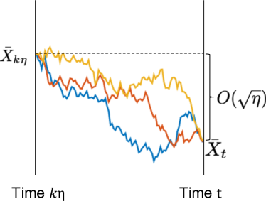
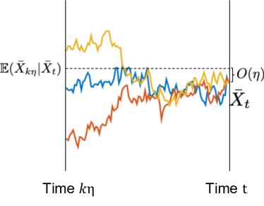
(a)		(b)

Figure 1: (a) Non-smooth initial distribution leads to $O(\sqrt{\eta})$ scaling. (b) Smooth initial distribution: Oscillation cancels and leads to $O(\eta)$ error.

Due to the dependence between $\hat{X}_{t}$ and Gaussian noise, we cannot expect cancellation to occur in general. Figure 1(a) illustrates an extremal case, where the initial distribution at time $k\eta$ is an atomic mass. When we condition on the value at $\hat{X}_{t}$ as well, the process behaves like a Brownian bridge. Consequently, it makes no difference whether the conditional expectation is inside or outside the norm: in either case, there is a term of the form $\|\hat{X}_{k\eta}-\hat{X}_{t}\|_{2}$, which scales as $O(\sqrt{\eta})$.

On the other hand, as illustrated in Figure 1(b), if the initial distribution is uniform over some region, the initial point is almost equally likely to be from anywhere around $\hat{X}_{t}$, up to the drift term, and most of the noise gets cancelled out. In general, if the initial distribution is smooth, locally it looks almost uniform, and similar phenomena should also hold true. Thus we expect $\mathbb{E}(\hat{X}_{k\eta}|\hat{X}_{t})-\hat{X}_{t}$ to be decomposed into terms coming from the drift and terms coming from the smoothness of the initial distribution.

4.2 Upper Bound via Integration by Parts

With this intuition in hand, we now turn to the proof itself. In order to leverage the smoothness of the initial distribution, we use integration by parts to move the derivatives onto the density of $\hat{X}_{k\eta}$. From Bayes’ formula, we have

$$\mathbb{E}\left(\hat{X}_{k\eta}\!-\!\hat{X}_{t}\big{|}\hat{X}_{t}\!=\!x\right)\!=\!\int(y\!-\!x)p(\hat{X}_{k\eta}\!=\!y|\hat{X}_{t}\!=\!x)dy\!=\!\int(y\!-\!x)\textstyle\frac{\hat{\pi}_{k\eta}(y)p(\hat{X}_{t}=x|\hat{X}_{k\eta}=y)}{\hat{\pi}_{t}(x)}dy.$$ (19)

Since the density $p(\hat{X}_{t}=x\mid\hat{X}_{k\eta}=y)$ is a Gaussian centered at $y-(t-k\eta)b(y)$ with fixed covariance, the gradient with respect to $y$ is the density itself times a linear factor $x-y+(t-k\eta)b(y)$, with an additional factor depending on the Jacobian of $b$. This elementary fact motivates a decomposition whose goal is to express $\mathbb{E}\left(\hat{X}_{k\eta}-\hat{X}_{t}\big{|}\hat{X}_{t}=x\right)$ as the sum of the conditional expectation of $\nabla\log\hat{\pi}_{k\eta}$ and some other terms which are easy to control. More precisely, in order to expose a gradient of the Gaussian density, we decompose the difference $y-x$ into three parts, namely $y-x=a_{1}(x,y)-a_{2}(x,y)-a_{3}(x,y)$, where

$$a_{1}(x,y) :=\left(I+(t-k\eta)\nabla b(y))(y-x+(t-k\eta)b(y)\right),$$

$$a_{2}(x,y) :=(t-k\eta)\nabla b(y)(y-x+(t-k\eta)b(y)),\quad\mbox{and}$$

$$a_{3}(x,y) :=(t-k\eta)b(y).$$

We define the conditional expectations $I_{i}(x):=\mathbb{E}\left(a_{i}(\hat{X}_{k\eta},\hat{X}_{t})\big{|}\hat{X}_{t}=x\right)$ for $i=1,2,3$ and control the three terms separately.

Let us denote by $\varphi$ the $d$-dimensional standard Gaussian density. The first term $I_{1}$ can directly be expressed in term of the gradient of $\varphi$:

$$I_{1}(x) =\int(I+(t-k\eta)\nabla b(y))(y-x+(t-k\eta)b(y))\varphi\left(\frac{x-y-(t-k\eta)b(y)}{\sqrt{t-k\eta}}\right)\frac{\hat{\pi}_{k\eta}(y)}{\hat{\pi}_{t}(x)}dy$$

$$=(t-k\eta)\int\nabla_{y}\varphi\left(\frac{x-y-(t-k\eta)b(y)}{\sqrt{t-k\eta}}\right)\frac{\hat{\pi}_{k\eta}(y)}{\hat{\pi}_{t}(x)}dy,$$

where we used the chain rule and $\nabla\varphi(y)=-y\varphi(y)$. Thus, applying integration by parts, we write $I_{1}$ in a revised form.

Lemma 4.

For all $t\in[k\eta,(k+1)\eta]$, we have

$$I_{1}(x)=-(t-k\eta)\mathbb{E}\left(\nabla\log\hat{\pi}_{k\eta}(\hat{X}_{k\eta})\big{|}\hat{X}_{t}=x\right),$$

and consequently,

$$\mathbb{E}\|I_{1}(\hat{X}_{t})\|_{2}^{2}\leq(t-k\eta)^{2}\int\hat{\pi}_{k\eta}(x)\|\nabla\log\hat{\pi}_{k\eta}(x)\|_{2}^{2}dx.$$

See Section 4.3 for the proof of this lemma.

It is clear from Lemma 4 that a regularity estimates on the moments of $\nabla\log\hat{\pi}_{k\eta}(\hat{X}_{k\eta})$ gives an $O(\eta^{2})$ estimates on the squared integral. Such a bound with reasonable dimension dependence is nontrivial to obtain. This is postponed to section 5.

The remaining two terms are relatively easy to control, as summarized in the following:

Lemma 5.

Under Assumption 1, the following bounds hold for all $t\in[k\eta,(k+1)\eta]$:

$$\mathbb{E}\|I_{2}(\hat{X}_{t})\|_{2}^{2} \leq 3(t-k\eta)^{3}L_{1}^{2}d,\quad\mbox{and}$$ (20a)

$$\mathbb{E}\|I_{3}(\hat{X}_{t})\|_{2}^{2} \leq 2\eta^{2}(A_{0}^{2}+L_{1}^{2}\mathbb{E}\|\hat{X}_{k\eta}\|_{2}^{2}).$$ (20b)

See Section 4.4 for the proof of this lemma.

Combining the Taylor expansion (18) with the bounds from Lemma 4 and 5 yields the bound claimed in Proposition 1.

4.3 Proof of Lemma 4

We prove here Lemma 4 which controls the dominant term $I_{1}$ of the decomposition of $\mathbb{E}\left(\hat{X}_{k\eta}\!-\!\hat{X}_{t}\big{|}\hat{X}_{t}\!=\!x\right)$ in (19). Recall $I_{1}$ is expressed in term of the gradient of the Gaussian density:

$$I_{1}(x) =(t-k\eta)\int\nabla_{y}\varphi\left(\frac{x-y-(t-k\eta)b(y)}{\sqrt{t-k\eta}}\right)\frac{\hat{\pi}_{k\eta}(y)}{\hat{\pi}_{t}(x)}dy,$$

where $\varphi$ is the $d$-dimensional standard Gaussian density. We first note the tail of the Gaussian density is trivial, and the tail of $\hat{\pi}_{k\eta}$ is justified by Appendix D. Therefore we obtain applying integration by parts:

$$I_{1}(x)= \int(I+(t-k\eta)\nabla b(y))(y-x+(t-k\eta)b(y))(2\pi(t-k\eta))^{-\frac{d}{2}}$$

$$\quad\quad\quad\quad\quad\cdot\exp\left(-\frac{1}{2(t-k\eta)}\|x-y-(t-k\eta)b(y)\|_{2}^{2}\right)\frac{\hat{\pi}_{k\eta}(y)}{\hat{\pi}_{t}(x)}dy$$

$$= \int(t-k\eta)\nabla_{y}\exp\left(-\frac{1}{2(t-k\eta)}\|x-y-(t-k\eta)b(y)\|_{2}^{2}\right)\frac{\hat{\pi}_{k\eta}(y)}{\hat{\pi}_{t}(x)}dy$$

$$= -(t-k\eta)\int\exp\left(-\frac{1}{2(t-k\eta)}\|x-y-(t-k\eta)b(y)\|_{2}^{2}\right)\frac{\nabla_{y}\hat{\pi}_{k\eta}(y)}{\hat{\pi}_{t}(x)}dy$$

$$= -(t-k\eta)\int\nabla_{y}\log\hat{\pi}_{k\eta}(y)p(\hat{X}_{t}=x|\hat{X}_{k\eta}=y)\frac{\hat{\pi}_{k\eta}(y)}{\hat{\pi}_{t}(x)}dy$$

$$= -(t-k\eta)\mathbb{E}\left(\nabla\log\hat{\pi}_{k\eta}(\hat{X}_{k\eta})\big{|}\hat{X}_{t}=x\right).$$

Then, applying the Cauchy-Schwartz inequality yields

$$\mathbb{E}\|I_{1}(\hat{X}_{t})\|_{2}^{2}= (t-k\eta)^{2}\mathbb{E}\left\|\mathbb{E}\left(\nabla\log\hat{\pi}_{k\eta}(\hat{X}_{k\eta})\big{|}\hat{X}_{t}\right)\right\|_{2}^{2}$$

$$\leq (t-k\eta)^{2}\mathbb{E}\|\nabla\log\hat{\pi}_{k\eta}(\hat{X}_{k\eta})\|_{2}^{2}=(t-k\eta)^{2}\int\hat{\pi}_{k\eta}\|\nabla\log\hat{\pi}_{k\eta}\|_{2}^{2}.$$

This last inequality concludes the proof of Lemma 4.

4.4 Proof of Lemma 5

Recall that this lemma provides bounds on the remaining two terms $I_{2}(x)$ and $I_{3}(x)$ of the decomposition of $\mathbb{E}\left(\hat{X}_{k\eta}\!-\!\hat{X}_{t}\big{|}\hat{X}_{t}\!=\!x\right)$ in (19). We split our proof into two parts, corresponding to the two bounds.

Proof of the bound (20a):

We directly bound the Jacobian matrix using Assumption 1.

$$\frac{\|I_{2}(x)\|_{2}}{t-k\eta} =\left\|\int\nabla b(y)(y-x+(t-k\eta)b(y))(2\pi(t-k\eta))^{-\frac{d}{2}}\exp\left(-\frac{\|x-y-(t-k\eta)b(y)\|_{2}^{2}}{2(t-k\eta)}\right)\frac{\hat{\pi}_{k\eta}(y)}{\hat{\pi}_{t}(x)}dy\right\|_{2}$$

$$\leq L_{1}\int\|(y-x+(t-k\eta)b(y)\|_{2}\frac{\hat{\pi}_{k\eta}(y)}{\hat{\pi}_{t}(x)}p(\hat{X}_{t}=x\big{|}\hat{X}_{k\eta}=y)dy$$

$$=L_{1}\mathbb{E}\left(\|\hat{X}_{k\eta}+(t-k\eta)b(\hat{X}_{k\eta})-\hat{X}_{t}\|_{2}\Big{|}\hat{X}_{t}=x\right)$$

$$=L_{1}\mathbb{E}\left(\|\int_{k\eta}^{t}dB_{s}\|_{2}\Big{|}\hat{X}_{t}=x\right).$$

Plugging into the squared integral yields

$$\mathbb{E}\|I_{2}(\hat{X}_{t})\|_{2}^{2}\leq(t-k\eta)^{2}L_{1}^{2}\mathbb{E}\left(\mathbb{E}\left(\|\int_{k\eta}^{t}dB_{s}\|\Big{|}\hat{X}_{t}\right)\right)^{2}\leq(t-k\eta)^{2}L_{1}^{2}\mathbb{E}\|\int_{k\eta}^{t}dB_{s}\|_{2}^{2}\leq 3(t-k\eta)^{3}L_{1}^{2}d.$$

Proof of the bound (20b):

The size of norm of $I_{3}$ is determined largely by $b(\hat{X}_{k\eta})$, which can be controlled using Assumption 1:

$$\mathbb{E}\|I_{3}(\hat{X}_{t})\|_{2}^{2}=(t-k\eta)^{2}\mathbb{E}\|\mathbb{E}(b(\hat{X}_{k\eta})|\hat{X}_{t})\|_{2}^{2}\leq\eta^{2}\mathbb{E}\|b(\hat{X}_{k\eta})\|_{2}^{2}\leq 2\eta^{2}(A_{0}^{2}+L_{1}^{2}\mathbb{E}\|\hat{X}_{k\eta}\|_{2}^{2}).$$

5 Regularity and Moment Estimates

From the previous section, we have upper bounded the time derivative of the KL divergence between the Langevin diffusion and its Euler discretization, using the Fisher information of $\pi_{k\eta}$ and the moment of $\hat{X}_{k\eta}$. In order to show that the above estimate is $O(\eta^{2})$, we derive, in the next section, upper bounds on the Fisher information and the moments which are independent of the step size.

Bounding the discretization error essentially relies on a $L^{2}$ estimate of $\nabla\log\hat{\pi}_{k\eta}$, and a higher order moment of $\hat{X}_{k\eta}$. In this section, we provide non-asymptotic bounds for both quantities. The regularity estimate is using a variant of the famous De Bruijn identity that relates Fisher information to entropy. This stands in sharp contrast to classical PDE regularity theory, which suffers from exponential dimension dependencies. The moment estimate comes from a standard martingale argument, but with explicit dependence on all the parameters.

5.1 Proof of Proposition 2

We now turn to the proof of Proposition 2, which gives a control on the Fisher information term needed by Proposition 1. We first bound the time integral of $\int\hat{\pi}_{t}\|\log\hat{\pi}_{t}\|_{2}^{2}$, and then relate it to the average at the grid points. The techniques introduced are novel and of independent interests.

The De Bruijn identity relates the time derivative of the KL divergence with the Fisher information for the heat kernel (Cover and Thomas, 2006). We establish an analogous result for the Fokker-Planck equation constructed in Lemma 1. This serves as a starting point of the regularity estimate used in this paper, though going from time integral to discrete grid points still takes effort.

Lemma 6.

For the time-marginal densities $\hat{\pi}_{t}$ of the interpolated process $\hat{X}_{t}$, we have:

$$\int_{0}^{T}\int\hat{\pi}_{t}(x)\|\nabla\log\hat{\pi}_{t}(x)\|_{2}^{2}dxdt\leq 4\left(h_{0}+\sigma_{0}^{-2}\mathbb{E}\|\hat{X}_{T}\|_{2}^{2}+H(\pi_{0})\right)+16\int_{0}^{T}\left(A_{0}^{2}+L_{1}^{2}\mathbb{E}\|\hat{X}_{t}\|_{2}^{2}\right)dt,$$

where $H(\cdot)$ denotes the differential entropy.

See Section 5.1.1 for the proof.

Lemma 6 gives control on the average of the second order regularity estimate. However, we want bound for this quantity evaluated at the grid points $\{k\eta\}_{k=1}^{+\infty}$. To relate back to grid points, we use to discrete-time arguments, by splitting the transformation from $\hat{\pi}_{t}$ to $\hat{\pi}_{k\eta}$ into two parts, and mimic the forward Euler algorithm. The following lemma gives control on the relative difference between the integral at time $k\eta$ and $t\in[(k-1)\eta,k\eta]$. The proof is postponed to Section 5.1.2.

Lemma 7.

For any $\eta\in\big{(}0,\frac{1}{2L_{1}}\big{)}$ and $t_{0}\in[(k-1)\eta,k\eta]$, we have:

$$\int\hat{\pi}_{k\eta}\|\nabla\log\hat{\pi}_{k\eta}\|_{2}^{2}\leq 8\int\hat{\pi}_{t_{0}}\|\nabla\log\hat{\pi}_{t_{0}}\|_{2}^{2}+32\eta^{2}d^{2}L_{2}^{2}.$$ (21)

Taking averages over $t_{0}\!\in\![(k\!-\!1)\eta,k\eta]$ in equation (21) and then summing over $k$ completes the proof of Proposition 2.

5.1.1 Proof of Lemma 6

Our general strategy is to relate the Laplacian operator in the semigroup generator, with the one that naturally comes from applying integration by parts to the Fisher information. Note that in the second step we use the divergence theorem, which is justified by Remark 1 in Appendix D.

$$\int\hat{\pi}\|\nabla\log\hat{\pi}\|_{2}^{2}=\int\langle\nabla\hat{\pi},\nabla\log\hat{\pi}\rangle=-\int\log\hat{\pi}\Delta\hat{\pi}.$$ (22)

On the other hand, the semigroup generator for the time-inhomogeneous process is given by

$$\hat{\mathcal{L}}_{t}\hat{\pi}=-\nabla\cdot\left(\hat{\pi}\hat{b}\right)+\frac{1}{2}\Delta\hat{\pi}.$$ (23)

Putting together equations (22) and (23) yields

$$\int\hat{\pi}\|\nabla\log\hat{\pi}\|_{2}^{2} =-2\int(\hat{\mathcal{L}}_{t}\hat{\pi})\log\hat{\pi}+2\int\nabla\cdot\left(\hat{\pi}\hat{b}\right)\log\hat{\pi}$$

$$=-2\int\frac{\partial\hat{\pi}}{\partial t}\log\hat{\pi}+2\int\nabla\cdot\left(\hat{\pi}\hat{b}\right)\log\hat{\pi}$$

$$= -2\frac{d}{dt}\left(\int\hat{\pi}\log\frac{\hat{\pi}}{\pi_{0}}\right)-2\frac{d}{dt}\mathbb{E}_{\hat{\pi}}\log\pi_{0}-2\int\hat{\pi}\left(\nabla\log\hat{\pi}\cdot\hat{b}\right)$$

$$\leq-2\frac{d}{dt}\left(\int\hat{\pi}\log\frac{\hat{\pi}}{\pi_{0}}\right)-2\frac{d}{dt}\mathbb{E}_{\hat{\pi}}\log\pi_{0}+4\int\hat{\pi}\|\hat{b}\|_{2}^{2}+\frac{1}{2}\int\hat{\pi}\|\nabla\log\hat{\pi}\|_{2}^{2}.$$

This directly yields to:

$$\int\hat{\pi}\|\nabla\log\hat{\pi}\|_{2}^{2}\leq-4\frac{d}{dt}\left(\int\hat{\pi}\log\frac{\hat{\pi}}{\pi_{0}}\right)-4\frac{d}{dt}\mathbb{E}_{\hat{\pi}}\log\pi_{0}+8\int\hat{\pi}\|\hat{b}\|_{2}^{2}.$$ (24)

Under Assumption 4, we have $-\mathbb{E}_{\hat{\pi}}\log\pi_{0}\leq h_{0}+\sigma_{0}^{-2}\mathbb{E}\|\hat{X}_{t}\|_{2}^{2}$. On the other hand, $\int\hat{\pi}\log\frac{\hat{\pi}}{\pi_{0}}=D_{\text{KL}}(\hat{\pi}\|\pi_{0})\geq 0$. Hence, plugging into (24) and integrating we obtain the desired result:

$$\int_{0}^{T}\int\hat{\pi}\|\nabla\log\hat{\pi}\|_{2}^{2}dt\leq 4\left(h_{0}+\sigma_{0}^{-2}\mathbb{E}\|\hat{X}_{T}\|_{2}^{2}+H(\pi_{0})\right)+16\int_{0}^{T}\left(A_{0}^{2}+L_{1}^{2}\mathbb{E}\|\hat{X}_{t}\|_{2}^{2}\right)dt.$$

5.1.2 Proof of Lemma 7

The proof involves a sequence of auxiliary lemmas. We first show that the transition from $\hat{\pi}_{t}$ to $\hat{\pi}_{k\eta}$ can be viewed as a discrete-time update.

Lemma 8.

For a given $t_{0}\in[(k-1)\eta,k\eta]$, define the random variable

$$\hat{Y}_{k\eta} :=\hat{X}_{t_{0}}+(k\eta-t_{0})\hat{b}_{t_{0}}(\hat{X}_{t_{0}})+(k\eta-t_{0})^{\frac{1}{2}}\mathcal{N}(0,I).$$ (25)

Then we have $\hat{Y}_{k\eta}\stackrel{{\scriptstyle d}}{{=}}\hat{X}_{k\eta}$.

Using Lemma 8, we can see $\hat{\pi}_{k\eta}$ as the consequence of a nonlinear transform and heat kernel performed on $\hat{\pi}_{t_{0}}$. For the first part, we can directly bound it, as long as $\eta$ is not too large:

Lemma 9.

Let $\phi:{}^{d}\rightarrow{}^{d},\phi(x)=x+(t-k\eta_{0})\hat{b}_{t_{0}}(x)$. For $\eta<\frac{1}{2L_{1}}$, Let $Z=\hat{X}_{t_{0}}+(k\eta-t_{0})\hat{b}_{t_{0}}(\hat{X}_{t_{0}})$, and let $p(\cdot)$ be the density of $Z$. We have:

$$\int p(z)\|\nabla_{z}\log p(z)\|_{2}^{2}dz\leq 8\int\hat{\pi}_{t_{0}}(x)\|\nabla_{x}\log\hat{\pi}_{t_{0}}(x)\|_{2}^{2}dx+32\eta^{2}d^{2}L_{2}^{2}.$$

The second term is harmless because it is of order $O(\eta^{2})$, leading to $O(\eta^{4})$ in the final bound, and the first term blows up the regularity estimate by factor 8.

In our next step, we are going to relate the $L^{2}$ regularity integral of $p$ to that of $\hat{\pi}_{k\eta}$, and therefore finish establishing the connection between the integral at grid points and at arbitrary time point.

First of all, we note the fact that the transition from $p$ to $\hat{\pi}_{k\eta}^{\prime}$ follows a heat equation in ^d. Concretely, consider the equation:

$$\frac{\partial u_{s}}{\partial s}(x)=\Delta u_{s}(x),\quad u_{t_{0}}(x)=p(x)\qquad\mbox{for all $x\in{}^{d}$},$$

with $s\in[t_{0},k\eta]$, the unique solution satisfies $u_{k\eta}=\hat{\pi}_{k\eta}^{\prime}=\hat{\pi}_{k\eta}$ according to Lemma 8. A nice property about Fisher information is that, it is non-increasing along the flow of heat kernel:

Lemma 10.

For the heat equation $\frac{\partial u_{t}}{\partial t}=\Delta u$ with $u_{0}\geq 0$, $\int u_{0}(x)dx=1$, and $u_{0}$ satisfying the conditions in Appendix D, we have that $\int_{{}^{d}}u_{t}(x)\|\log u_{t}(x)\|dx$ is non-increasing in $t$.

Since $\eta\in(0,\frac{1}{2L_{1}}]$ by assumption, for $t_{0}\in[(k-1)\eta,k\eta]$, we obtain:

$$\int\hat{\pi}_{k\eta}\|\nabla\log\hat{\pi}_{k\eta}\|_{2}^{2}\leq\int p\|\nabla\log p\|_{2}^{2}\leq 8\int\hat{\pi}_{t_{0}}\|\nabla\log\hat{\pi}_{t_{0}}\|_{2}^{2}+32\eta^{2}d^{2}L_{2}^{2},$$ (26)

which completes the proof of Lemma 7.

5.2 Moment Estimate under Dissipative Assumption

In this section, we bound the moments of the process $\hat{X}_{k\eta}$ along the path of the discretized Langevin diffusion. In order to do so, we leverage Assumption 3, as stated in the following:

Lemma 11.

Suppose that Assumptions 3 and 4 hold for the interpolated process (12). Then there is a universal constant $C>0$ such that

$$\sup_{t\geq 0}\left(\mathbb{E}\|\hat{X}_{t}\|_{2}^{p}\right)^{\frac{1}{p}}\leq C\left(\sigma_{0}\sqrt{pd}+\sqrt{\frac{p+\beta+d}{\mu}}\right)\qquad\mbox{for all $p\geq 1$.}$$ (27)

The proof of this lemma is based on martingale $L^{p}$ estimates and the Burkholder-Davis-Gundy inequality (Burkholder et al., 1972). The details are postponed to Appendix B.3. It is worth noting the bound depends polynomially on the parameters $(\mu,\beta)$ in Assumption 3.

Without Assumption 3 and control on the directions of the drift at a far distance, the moment of the iterates can exponentially blow up. A simple counterexample is to let the potential function be $U(x)=-\|x\|_{2}^{2}$ and $b(x)=x$. Then it is easy to see that $\|\hat{X}_{t}\|_{2}\gtrsim e^{T}$ in this setup. this exponential growth, However Assumption 3 can actually be significantly weakened—as long as the potential function is non-negative. This comes at the cost of a worse dependence (still polynomial) on $T$.

5.3 Moment Estimates without Dissipative Assumptions

Note that Lemma 11 requires the distant dissipative assumption 3. This assumption can be relaxed with a slightly worse dependence on $T$, as long as the potential function is non-negative. In this section, we assume $b=-\nabla f$ with $f(x)\geq 0$ for any $x\in{}^{d}$. Under these conditions, we have the following:

Lemma 12.

Suppose Assumption 4 and 1 holds, for the process (12) with $b=-\nabla f$ and $f\geq 0$, there is a universal constant $C>0$, such that:

$$\sup_{0\leq k\leq T/\eta}\left({\mathbb{E}}\left\|\hat{X}_{k\eta}\right\|_{2}^{4}\right)\leq C\cdot\left(f(0)^{2}+L_{1}^{2}T^{2}\sigma_{0}^{4}(h_{0}+d)^{2}+L_{1}^{2}T^{4}d^{2}\right),$$

for some universal constant $C>0$.

By plugging the fourth moment obtained by Lemma 12 into Propostion 1 and Proposition 2, Theorem 2 can then be established.

5.3.1 Proof of Lemma 12

In this section, we present the proof of the moment bound given in Lemmas 12.

Let the process $\tilde{X}_{t}$ be the time-inhomogeneous diffusion process defined by generator $-\langle\hat{b}_{t},\,\nabla\rangle+\frac{1}{2}\Delta$, starting from $\hat{X}_{0}$. By Lemma 1, the one-time marginal laws of $\tilde{X}_{t}$ and $\hat{X}_{t}$ are the same. So we only need to show the moment bounds for $\tilde{X}_{t}$.

By Itô’s formula, we have:

$$\left\|\tilde{X}_{t}\right\|_{2}^{2}=\left\|\tilde{X}_{0}\right\|_{2}^{2}-2\int_{0}^{t}\langle\tilde{X}_{s},\,\hat{b}_{s}(\tilde{X}_{s})\rangle ds+2\int_{0}^{t}\langle\tilde{X}_{s},\,dB_{s}\rangle+td.$$

Taking expectation for both sides, we obtain:

$${\mathbb{E}}\left\|\tilde{X}_{t}\right\|_{2}^{2}\leq {\mathbb{E}}\left\|\tilde{X}_{0}\right\|_{2}^{2}+2\int_{0}^{t}{\mathbb{E}}\left(\left\|\tilde{X}_{s}\right\|_{2}\cdot\left\|\hat{b}_{s}(\tilde{X}_{s})\right\|_{2}\right)ds+td$$

$$\leq {\mathbb{E}}\left\|\tilde{X}_{0}\right\|_{2}^{2}+2\left(\int_{0}^{t}{\mathbb{E}}\left\|\tilde{X}_{s}\right\|_{2}^{2}ds\right)^{\frac{1}{2}}\left(\int_{0}^{t}{\mathbb{E}}\left\|\hat{b}_{s}(\tilde{X}_{s})\right\|_{2}^{2}ds\right)^{\frac{1}{2}}+td$$

$$\leq {\mathbb{E}}\left\|\tilde{X}_{0}\right\|_{2}^{2}+2\left(\int_{0}^{t}{\mathbb{E}}\left\|\tilde{X}_{s}\right\|_{2}^{2}ds\right)^{\frac{1}{2}}\left(\eta\sum_{k=0}^{t/\eta}{\mathbb{E}}\left\|\nabla f(\tilde{X}_{k\eta})\right\|_{2}^{2}\right)^{\frac{1}{2}}+td.$$

If an upper bound on average mean squared norm of $\nabla f(\hat{X}_{k\eta})$ can be obtained, the conclusion directly follows from solving an ordinary differential inequalities using variants of Grönwall lemma. Therefore, we need the following lemma about the squared gradient norms:

Lemma 13.

Suppose Assumption 1 and Assumption 4 holds, for the process (12) with $b=-\nabla f,~{}f\geq 0$ and $\eta<1/2L_{1}$, there is a universal constant $C>0$, such that:

$${\mathbb{E}}\eta\sum_{k=0}^{T/\eta}\left\|\nabla f(\hat{X}_{k\eta})\right\|_{2}^{2}\leq 2{\mathbb{E}}f(\hat{X}_{0})+L_{1}Td,$$

$${\mathbb{E}}\left(\eta\sum_{k=0}^{T/\eta}\left\|\nabla f(\hat{X}_{k\eta})\right\|_{2}^{2}\right)^{2}\leq 12{\mathbb{E}}f(\hat{X}_{0})^{2}+24{\mathbb{E}}f(\hat{X}_{0})+12TL_{1}d+9L_{1}^{2}T^{2}d^{2}.$$

The proof of this lemma is postponed to Appendix B.4. The main idea of the proof is straightforward: large norm of $\nabla f$ will force the value of $f$ to go down along the dynamics of Langevin algorithm. Since $f$ is non-negative, the average mean squared norm can be bounded using the initial value of $f$. However, the Gaussian noise is non-trivial to deal with. The combinatorial techniques used in the proof of Lemma 13 are only able to deal with up to fourth moment. Fortunately, this is what the proof of Theorem 2 needs.

Plugging the first bound in Lemma 12 into above upper bound for ${\mathbb{E}}\left\|\tilde{X}_{t}\right\|_{2}^{2}$, and taking supremum with $t\in[0,T]$ for both sides, we obtain:

$$\sup_{0\leq t\leq T}{\mathbb{E}}\left\|\tilde{X}_{t}\right\|_{2}^{2}\leq {\mathbb{E}}\left\|\tilde{X}_{0}\right\|_{2}^{2}+2\sqrt{(2{\mathbb{E}}f(\tilde{X}_{0})+L_{1}Td)\int_{0}^{T}{\mathbb{E}}\left\|\tilde{X}_{s}\right\|_{2}^{2}ds}+Td$$

$$\leq {\mathbb{E}}\left\|\tilde{X}_{0}\right\|_{2}^{2}+2\sqrt{(2{\mathbb{E}}f(\tilde{X}_{0})+L_{1}Td)T\sup_{0\leq t\leq T}{\mathbb{E}}\left\|\tilde{X}_{s}\right\|_{2}^{2}ds}+Td.$$

Solving the quadratic equation, we obtain:

$$\sup_{0\leq t\leq T}{\mathbb{E}}\left\|\tilde{X}_{t}\right\|_{2}^{2}\leq 2{\mathbb{E}}\left\|\tilde{X}_{0}\right\|_{2}^{2}+4T({\mathbb{E}}f(\tilde{X}_{0})+L_{1}Td)+2Td.$$

For the fourth moment, using Young’s inequality, we obtain:

$${\mathbb{E}}\left\|\tilde{X}_{t}\right\|_{2}^{4}\leq 4{\mathbb{E}}\left\|\tilde{X}_{0}\right\|_{2}^{4}+16\underbrace{{\mathbb{E}}\left(\int_{0}^{t}\langle\tilde{X}_{s},\,\hat{b}_{s}(\tilde{X}_{s})\rangle ds\right)^{2}}_{T_{1}}+16\underbrace{{\mathbb{E}}\left(\int_{0}^{t}\langle\tilde{X}_{s},\,dB_{s}\rangle\right)^{2}}_{T_{2}}+4t^{2}d^{2}.$$

For $T_{1}$, applying the Cauchy-Schwartz inequality multiple times, we have:

$$T_{1}\leq {\mathbb{E}}\left(\int_{0}^{t}\left\|\tilde{X}_{s}\right\|_{2}\cdot\left\|\hat{b}_{s}(\tilde{X}_{s})\right\|_{2}ds\right)^{2}$$

$$\leq {\mathbb{E}}\left(\int_{0}^{t}\left\|\tilde{X}_{s}\right\|_{2}^{2}ds\cdot\int_{0}^{t}\left\|\hat{b}_{s}(\tilde{X}_{s})\right\|_{2}^{2}ds\right)$$

$$\leq \left({\mathbb{E}}\left(\int_{0}^{t}\left\|\tilde{X}_{s}\right\|_{2}^{2}ds\right)^{2}\right)^{\frac{1}{2}}\cdot\left({\mathbb{E}}\left(\int_{0}^{t}\left\|\hat{b}_{s}(\tilde{X}_{s})\right\|_{2}^{2}ds\right)^{2}\right)^{\frac{1}{2}}$$

$$\leq \left(t\int_{0}^{t}{\mathbb{E}}\left\|\tilde{X}_{s}\right\|_{2}^{4}ds\right)^{\frac{1}{2}}\left({\mathbb{E}}\left(\eta\sum_{k=0}^{t/\eta}\left\|\nabla f(X_{k\eta})\right\|_{2}^{2}\right)^{2}\right)^{\frac{1}{2}}$$

$$\leq 12(\sqrt{{\mathbb{E}}f(\tilde{X}_{0})^{2}}+L_{1}Td)\left(t\int_{0}^{t}{\mathbb{E}}\left\|\tilde{X}_{s}\right\|_{2}^{4}ds\right)^{\frac{1}{2}}$$

For $T_{2}$, combining the Itô isometry with above bounds on the expected norm yields

$$T_{2}=\int_{0}^{t}{\mathbb{E}}\left\|\tilde{X}_{s}\right\|_{2}^{2}ds\leq 2t{\mathbb{E}}\left\|\tilde{X}_{0}\right\|_{2}^{2}+4t(t{\mathbb{E}}f(\tilde{X}_{0})+t^{2}L_{1}d)+2t^{2}d.$$

Similar to the second moment, by taking supremum over time, we obtain

$$\sup_{0\leq t\leq T}{\mathbb{E}}\left\|\tilde{X}_{t}\right\|_{2}^{4}\leq 4{\mathbb{E}}\left\|\tilde{X}_{0}\right\|_{2}^{4}+192\left(\sqrt{{\mathbb{E}}f(\tilde{X}_{0})^{2}}+L_{1}Td\right)\left(T\int_{0}^{T}{\mathbb{E}}\left\|\tilde{X}_{s}\right\|_{2}^{4}ds\right)^{\frac{1}{2}}\\ +16\left(2T{\mathbb{E}}\left\|\tilde{X}_{0}\right\|_{2}^{2}+4T(T{\mathbb{E}}f(\tilde{X}_{0})+T^{2}L_{1}d)+2T^{2}d\right)+4T^{2}d^{2}\\ \leq C\cdot{\mathbb{E}}\left\|\tilde{X}_{0}\right\|_{2}^{4}+CT\left(\sqrt{{\mathbb{E}}f(\tilde{X}_{0})^{2}}+L_{1}Td\right)\sqrt{\sup_{0\leq t\leq T}{\mathbb{E}}\left\|\tilde{X}_{s}\right\|_{2}^{4}}\\ +C\left(T{\mathbb{E}}\left\|\tilde{X}_{0}\right\|_{2}^{2}+T^{2}{\mathbb{E}}f(\tilde{X}_{0})+T^{3}L_{1}d+T^{2}d^{2}\right).$$

Solving the quadratic equation yields

$$\sup_{0\leq t\leq T}{\mathbb{E}}\left\|\tilde{X}_{s}\right\|_{2}^{4} \leq C\cdot{\mathbb{E}}\left\|\tilde{X}_{0}\right\|_{2}^{4}+CT^{2}\left({\mathbb{E}}f(\tilde{X}_{0})^{2}+L_{1}^{2}T^{2}d^{2}\right)+CT{\mathbb{E}}\left\|\tilde{X}_{0}\right\|_{2}^{2}$$

$$\leq C^{\prime}\cdot\left(f(0)^{2}+L_{1}^{2}T^{2}{\mathbb{E}}\left\|\tilde{X}_{0}\right\|_{2}^{4}+L_{1}^{2}T^{4}d^{2}\right)$$

$$\leq C^{\prime}\cdot\left(f(0)^{2}+L_{1}^{2}T^{2}\sigma_{0}^{2}(h_{0}+d)^{2}+L_{1}^{2}T^{4}d^{2}\right),$$

which completes the proof.

6 Discussion

We have presented an improved non-asymptotic analysis of the Euler-Maruyama discretization of the Langevin diffusion. We have shown that, as long as the drift term is second-order smooth, the KL divergence between the Langevin diffusion and its discretization is bounded as $O(\eta^{2}d^{2}T)$. Importantly, this analysis obtains the tight $O(\eta)$ rate for the Euler-Maruyama scheme (under Wasserstein or TV distances), without assuming global contractivity. This result serves as a convenient tool for the future study of Langevin algorithms for sampling, optimization, and statistical inference, as it allows to directly translate continuous-time results into discrete time, with tight rates.

Note that our results only apply to the Langevin diffusion. Considering the discretization of more general diffusions, either with location-varying covariance or second-order derivatives as the underdamped Langevin dynamics (Cheng et al., 2018b) is a promising direction for further research.

Acknowledgements

This work was partially supported by Office of Naval Research Grant ONR-N00014-18-1-2640 to MJW and National Science Foundation Grant NSF-CCF-1909365 to PLB and MJW. We also acknowledge support from National Science Foundation grant NSF-IIS-1619362 to PLB. We thank Xiang Cheng, Yi-An Ma and Andre Wibisono for helpful discussions.

Appendix A Proofs omitted from Section 4

In this section, we collect the proofs of results from Section 4; in particular, these results involve bounds on the derivative $\frac{d}{dt}D_{\text{KL}}(\hat{\pi}_{t}\|\pi_{t})$.

A.1 Proof of Lemma 2

In order to bound the derivative of the KL divergence, we first need to interchange the order of time derivative and the integration for KL divergence. Note that

$$\frac{\partial}{\partial t}\left(\hat{\pi}\log\frac{\hat{\pi}}{\pi}\right) =\hat{\pi}\left(\frac{\partial\log\hat{\pi}}{\partial t}(\log\hat{\pi}+1-\log\pi)-\frac{\partial\log\pi}{\partial t}\right)$$

$$=\hat{\pi}\cdot\mathrm{poly}(\nabla\log\hat{\pi},\Delta\log\hat{\pi},\nabla\log{\pi},\Delta\log\pi,b,\hat{b}).$$

From Lemma 14, the density $\hat{\pi}$ has a rapidly decaying tail, and the factor grows polynomially with $y$, uniformly in a small neighborhood of $t$. Therefore, the integrand admits a $L^{1}$ integrable dominating function over a small neighborhood of $t$. By the dominated convergence theorem, we can exchange the order of derivative and integration, thereby obtaining

$$\frac{d}{dt}D_{\text{KL}}(\hat{\pi}\|\pi)=\int_{{}^{d}}\frac{\partial}{\partial t}\left(\hat{\pi}\log\frac{\hat{\pi}}{\pi}\right)dx=\int_{{}^{d}}\frac{\partial\hat{\pi}}{\partial t}(\log\hat{\pi}+1-\log\pi)dx-\int_{{}^{d}}\frac{\partial\pi}{\partial t}\frac{\hat{\pi}}{\pi}dx.$$ (28)

For the first term, by Remark 1, we can apply the divergence theorem, and obtain:

$$\int_{{}^{d}}\frac{\partial\hat{\pi}}{\partial t}(\log\hat{\pi}+1-\log\pi)dx= \int_{{}^{d}}\left(\nabla\cdot(\hat{-\pi}\hat{b})+\frac{1}{2}\Delta\hat{\pi}\right)(\log\hat{\pi}+1-\log\pi)dx$$

$$=-\int_{{}^{d}}\left(-\hat{\pi}\hat{b}+\frac{1}{2}\nabla\hat{\pi}\right)\cdot(\nabla\log\hat{\pi}-\nabla\log\pi)dx.$$

Turning to the second term, by divergence theorem justified in Remark 1, we also have:

$$\int_{{}^{d}}\frac{\partial\pi}{\partial t}\frac{\hat{\pi}}{\pi}dx =\int_{{}^{d}}\left(-\nabla\cdot(\pi b)+\frac{1}{2}\Delta\pi\right)\frac{\hat{\pi}}{\pi}dx$$

$$=-\int_{{}^{d}}\left(-\pi b+\frac{1}{2}\nabla\pi\right)\cdot(\nabla\log\hat{\pi}-\nabla\log\pi)\frac{\hat{\pi}}{\pi}dx.$$

Putting together the pieces yields

$$\frac{d}{dt}D_{\text{KL}}(\hat{\pi}\|\pi) =-\int_{{}^{d}}\left(-\hat{\pi}\hat{b}+\frac{1}{2}\nabla\hat{\pi}\right)\cdot(\nabla\log\hat{\pi}-\nabla\log\pi)-\hat{\pi}\left(-b+\frac{1}{2}\nabla\log\pi\right)\cdot(\nabla\log\hat{\pi}-\nabla\log\pi)dx$$

$$=\int_{{}^{d}}\hat{\pi}(\nabla\log\hat{\pi}-\nabla\log\pi)\cdot(\hat{b}-b)dx-\frac{1}{2}\int_{{}^{d}}\hat{\pi}\|\nabla\log\hat{\pi}-\nabla\log\pi\|_{2}^{2}dx$$

$$\overset{(i)}{\leq}\frac{1}{2}\int_{{}^{d}}\hat{\pi}\|\hat{b}-b\|_{2}^{2}dx,$$

where step (i) uses Young’s inequality (namely, $u\cdot v\leq\frac{1}{2}u^{2}+\frac{1}{2}v^{2}$).

A.2 Proof of Lemma 3

We prove now Lemma 3, which gives a bound on the reminder term $\hat{r}_{t}$ of the Taylor series expansion (18). Let us consider the norm of $\hat{r}_{t}$ and apply the triangle inequality:

$$\|\hat{r}_{t}(x)\|_{2} =\left\|\mathbb{E}\left(\int_{0}^{1}s\nabla^{2}b((1-s)\hat{X}_{t}+s\hat{X}_{k\eta})[\hat{X}_{k\eta}-\hat{X}_{t},\hat{X}_{k\eta}-\hat{X}_{t}]ds\Big{|}\hat{X}_{t}=x\right)\right\|_{2}$$

$$\leq\int_{0}^{1}\mathbb{E}\left(|\!|\!|\nabla^{2}b((1-s)\hat{X}_{t}+s\hat{X}_{k\eta})|\!|\!|_{{\tiny{\mbox{op}}}}\cdot\|\hat{X}_{k\eta}-\hat{X}_{t}\|_{2}^{2}\Big{|}\hat{X}_{t}=x\right)$$

$$\leq\frac{L_{2}}{2}\mathbb{E}\left(\|\hat{X}_{k\eta}-\hat{X}_{t}\|_{2}^{2}\Big{|}\hat{X}_{t}=x\right)$$

$$\leq L_{2}\mathbb{E}\left(\|(t-k\eta)b(\hat{X}_{k\eta})\|_{2}^{2}+\left\|\int_{k\eta}^{t}dB_{s}\right\|_{2}^{2}\Big{|}\hat{X}_{t}=x\right).$$

Taking the global expectation leads to

$$\mathbb{E}\|\hat{r}_{t}(\hat{X}_{t})\|_{2}^{2}\leq L_{2}^{2}\mathbb{E}\mathbb{E}\left(\|(t-k\eta)b(\hat{X}_{k\eta})\|_{2}^{2}+\left\|\int_{k\eta}^{t}dB_{s}\right\|_{2}^{2}\Big{|}\hat{X}_{t}\right)^{2}$$

$$\stackrel{{\scriptstyle(i)}}{{\leq}} L_{2}^{2}\mathbb{E}\left(\|(t-k\eta)b(\hat{X}_{k\eta})\|_{2}^{2}+\left\|\int_{k\eta}^{t}dB_{s}\right\|_{2}^{2}\right)^{2}$$

$$\stackrel{{\scriptstyle(ii)}}{{\leq}} 2L_{2}^{2}\mathbb{E}\left(\|(t-k\eta)b(\hat{X}_{k\eta})\|_{2}^{4}+\left\|\int_{k\eta}^{t}dB_{s}\right\|_{2}^{4}\right)$$

$$\leq 8(t-k\eta)^{4}L_{2}^{2}\left(A_{0}^{4}+L_{1}^{4}\mathbb{E}\|\hat{X}_{k\eta}\|_{2}^{4}\right)+24(t-k\eta)^{2}L_{2}^{2}d^{2},$$

where step (i) follows from the Cauchy-Schwartz inequality; and step (ii) follows from a variant of Young’s inequality (namely, $(a+b)^{2}\leq 2(a^{2}+b^{2})$).

Appendix B Proofs Omitted from Section 5

In this section, we present the proofs omitted from Section 5. In particular, these results involve upper bounds on the Fisher information and the moments.

B.1 Proof of Lemma 8

We first construct an interpolated process:

$$\hat{X}_{s}^{\prime}=\hat{X}_{t_{0}}+(s-t_{0})\hat{b}_{t_{0}}(\hat{X}_{t_{0}})+\int_{t_{0}}^{s}dB_{t},\quad\forall s\in[t_{0},k\eta].$$ (29)

According to Lemma 1, the density $\hat{\pi}^{\prime}_{s}$ of $\hat{X}_{s}^{\prime}$ satisfies the following Fokker-Planck equation:

$$\frac{\partial\hat{\pi}_{t}^{\prime}}{\partial s}(x)=\nabla\cdot\left(\hat{\pi}_{t}^{\prime}(x)\mathbb{E}\left(\hat{b}_{t_{0}}(\hat{X}_{t_{0}})\big{|}\hat{X}_{s}=x\right)\right)+\frac{1}{2}\Delta\hat{\pi}_{t}^{\prime}(x).$$ (30)

Note that for $(k-1)\eta\leq t_{0}\leq s$, we have:

$$\mathbb{E}\left(\hat{b}_{t_{0}}(\hat{X}_{t_{0}})\big{|}\hat{X}_{s}=x\right)=\mathbb{E}\left(\mathbb{E}\left(b(\hat{X}_{(k-1)\eta})\big{|}\hat{X}_{t_{0}}\right)\Big{|}\hat{X}_{s}=x\right)=\mathbb{E}\left(b(\hat{X}_{(k-1)\eta})\big{|}\hat{X}_{s}=x\right)=\hat{b}_{s}(x).$$ (31)

Plugging back into the Fokker-Planck equation, we get:

$$\frac{\partial\hat{\pi}_{t}^{\prime}}{\partial s}(x)=\nabla\cdot\left(\hat{\pi}_{t}^{\prime}(x)\hat{b}_{s}(x)\right)+\frac{1}{2}\Delta\hat{\pi}_{t}^{\prime}(x),$$ (32)

which is exactly the same PDE as in Lemma 1. Due to the uniqueness of solution to parabolic equations, we have:

$$\hat{\pi}_{s}=\hat{\pi}_{s}^{\prime},\quad\forall s\in[t_{0},k\eta],$$ (33)

which proves the lemma.

B.2 Proof of Lemma 9

For $\eta\in(0,\frac{1}{2L_{1}})$, it is easy to see that $\phi$ is a one-to-one mapping, and $\frac{1}{2}I\preceq\nabla\phi\preceq\frac{3}{2}I$.

$$\int p(z)\|\nabla_{z}\log p(z)\|_{2}^{2}dz= \int p(\phi(x))\|\nabla_{z}\log p(\phi(x))\|_{2}^{2}\det(\nabla\phi(x))dx$$

$$= \int p(\phi(x))\|\nabla\phi(x)^{-1}\nabla_{x}\log p(\phi(x))\|_{2}^{2}\det(\nabla\phi(x))dx$$

$$= \int\hat{\pi}_{t_{0}}(x)\|\nabla\phi(x)^{-1}\left(\nabla_{x}\log\hat{\pi}_{t_{0}}(x)-\nabla\log\det(\nabla\phi(x))\right)\|_{2}^{2}dx$$

$$\leq 2\int\hat{\pi}_{t_{0}}(x)\|\nabla\phi(x)^{-1}\nabla_{x}\log\hat{\pi}_{t_{0}}(x)\|_{2}^{2}dx$$

$$\quad+2\int\hat{\pi}_{t_{0}}(x)\|\nabla\phi(x)^{-1}\nabla\log\det(\nabla\phi(x))\|_{2}^{2}dx$$

$$\leq 8\int\hat{\pi}_{t_{0}}(x)\|\nabla_{x}\log\hat{\pi}_{t_{0}}(x)\|_{2}^{2}dx+32\eta^{2}d^{2}L_{2}^{2}.$$

For the last inequality, the first term is due to $|\!|\!|\nabla\phi(x)^{-1}|\!|\!|_{{\tiny{\mbox{op}}}}\leq 2$, and the bound for second term can be derived as:

$$\int\hat{\pi}_{t_{0}}(x)\|\nabla\phi(x)^{-1}\nabla\log\det(\nabla\phi(x))\|_{2}^{2}dx =\int\hat{\pi}_{t_{0}}(x)\|\nabla\phi(x)^{-2}\nabla\cdot(I+(k\eta-t_{0})\nabla\hat{b}_{t_{0}}(x))\|_{2}^{2}dx$$

$$\leq 16\eta^{2}d^{2}L_{2}^{2}.$$

B.2.1 Proof of Lemma 10

Let $\phi_{t}$ be the density of $d$-dimensional Gaussian with mean 0 and covariance $tI_{d}$. Apparently $u_{t}=u_{0}\star\phi_{t}$. Note that by Cauchy-Schwartz inequality,

$$\int u_{t}\left\|\nabla\log u_{t}\right\|_{2}^{2}dx =\int u_{0}\star\phi_{t}(x)\left\|\frac{\int\nabla\log u_{0}(x-y)u_{0}(x-y)\phi_{t}(y)dy}{\int u_{0}(x-y)\phi_{t}(y)dy}\right\|_{2}^{2}dx$$

$$\leq\int u_{0}\star\phi_{t}(x)\frac{\int\left\|\nabla\log u_{0}(x-y)\right\|_{2}^{2}u_{0}(x-y)\phi_{t}(y)dy}{\int u_{0}(x-y)\phi_{t}(y)dy}dx$$

$$=\int\int\left\|\nabla\log u_{0}(x-y)\right\|_{2}^{2}u_{0}(x-y)\phi_{t}(y)dydx$$

$$=\int\left\|\nabla\log u_{0}(z)\right\|_{2}^{2}u_{0}(z)\left(\int\phi_{t}(y)dy\right)dz$$

$$=\int\left\|\nabla\log u_{0}(z)\right\|_{2}^{2}u_{0}(z)dz,$$

which finishes the proof.

B.3 Proof of Lemma 11

In this section, we present the proof of the moment bound given in Lemmas 11. Let the process $\tilde{X}_{t}$ be the time-inhomogeneous diffusion process defined by generator $-\langle\hat{b}_{t},\,\nabla\rangle+\frac{1}{2}\Delta$, starting from $\hat{X}_{0}$. By Lemma 1, the one-time marginal laws of $\tilde{X}_{t}$ and $\hat{X}_{t}$ are the same. So we only need to show the moment bounds for $\tilde{X}_{t}$.

We first apply Itô’s formula, for some $c>0$, and obtain:

$$\frac{1}{2}e^{ct}\|\tilde{X}_{t}\|_{2}^{2}-\frac{1}{2}\|\tilde{X}_{0}\|_{2}^{2}=\int_{0}^{t}\langle\tilde{X}_{s},\hat{b}(\tilde{X}_{s})e^{cs}\rangle ds+\frac{d}{2}\int_{0}^{t}e^{cs}ds\\ +\int_{0}^{t}e^{cs}\tilde{X}_{s}^{T}dB_{s}+\frac{1}{2}\int_{0}^{t}ce^{cs}\|\tilde{X}_{s}\|_{2}^{2}ds.$$

Letting $\hat{M}_{t}:=\int_{0}^{t}\tilde{X}_{s}^{T}e^{cs}dB_{s}$ be the martingale term, using the Burkholder-Gundy-Davis inequality (Burkholder et al., 1972), for $p\geq 4$, we have:

$$\mathbb{E}\sup_{0\leq t\leq T}|M_{t}|^{\frac{p}{2}} \leq(pC)^{\frac{p}{4}}\mathbb{E}\langle M,M\rangle_{T}^{\frac{p}{4}}$$

$$\leq (pC)^{\frac{p}{4}}\mathbb{E}\left(\int_{0}^{T}e^{2cs}\|\tilde{X}_{s}\|_{2}^{2}ds\right)^{\frac{p}{4}}$$

$$\leq(pC)^{\frac{p}{4}}\mathbb{E}\left(\sup_{0\leq s\leq T}e^{cs}\|\tilde{X}_{s}\|_{2}^{2}\cdot\int_{0}^{T}e^{cs}ds\right)^{\frac{p}{4}} \leq\left(\frac{Cpe^{cT}}{c}\right)^{\frac{p}{4}}\left(A+\frac{1}{A}\mathbb{E}\left(\sup_{0\leq t\leq T}e^{ct}\|\tilde{X}_{t}\|_{2}^{2}\right)^{\frac{p}{2}}\right).$$

Note that this bound holds for an arbitrary value of $A>0$; we make a specific choice later in the argument. On the other hand, by Assumption 3, we have:

$$\int_{0}^{t}\langle\tilde{X}_{s},\hat{b}(\tilde{X}_{s})e^{cs}\rangle ds\leq\int_{0}^{t}\left(-\mu\|\tilde{X}_{s}\|_{2}^{2}+\beta\right)e^{cs}ds.$$ (34)

Putting these bounds together with $c=2\mu$, we find that

$$\mathbb{E}\left(\sup_{0\leq t\leq T}e^{2\mu t}\|\tilde{X}_{t}\|_{2}^{2}\right)^{\frac{p}{2}}\leq 3^{\frac{p}{2}-1}\mathbb{E}\|X_{0}\|_{2}^{p}+3^{\frac{p}{2}-1}\mathbb{E}\sup_{0\leq t\leq T}|M_{t}|^{\frac{p}{2}}$$

$$+3^{\frac{p}{2}-1}\mathbb{E}\left(\sup_{0\leq t\leq T}\int_{0}^{t}\left(2\langle\tilde{X}_{s},\hat{b}(\tilde{X}_{s})\rangle+d+c\|\tilde{X}_{s}\|_{2}^{2}\right)e^{cs}ds\right)^{\frac{p}{2}}$$

$$\leq (C\sigma_{0}^{2}pd)^{\frac{p}{2}}+\left(\frac{Cpe^{2\mu T}}{\mu}\right)^{\frac{p}{4}}\left(A+\frac{1}{A}\mathbb{E}\left(\sup_{0\leq t\leq T}e^{2\mu t}\|\tilde{X}_{t}\|_{2}^{2}\right)^{\frac{p}{2}}\right)$$

$$+3^{\frac{p}{2}-1}\mathbb{E}\left(\sup_{0\leq t\leq T}\int_{0}^{t}\left(2\beta+d\right)e^{2\mu s}ds\right)^{\frac{p}{2}},$$

for some universal constant $C>0$.

Setting $A=2\left(\frac{Cpe^{2\mu T}}{\mu}\right)^{\frac{p}{4}}$ and substiuting into the inequality above, we find that

$$\left(\mathbb{E}\|\tilde{X}_{T}\|_{2}^{p}\right)^{\frac{1}{p}}\leq e^{-\mu T}\left(\mathbb{E}\left(\sup_{0\leq t\leq T}e^{2\mu t}\|\hat{X}_{t}\|_{2}^{2}\right)^{\frac{p}{2}}\right)^{\frac{1}{p}}\leq C^{\prime}\left(e^{-\mu T}\sigma_{0}\sqrt{pd}+\sqrt{\frac{p}{\mu}}+\sqrt{\frac{2\beta+d}{\mu}}\right),$$ (35)

for universal constant $C^{\prime}>0$, which proves the claim.

B.4 Proof of Lemma 13

A key technical ingredient in the proof of Lemma 12 is Lemma 13, which bound the second and fourth moments of gradient along the path of the Euler-Maruyama scheme with non-negative potential functions. It is worth noticing that the exact cancellation needed in the proof only happens with the first and second moment of average squared gradient norm, which is exactly what we need for the proof of Theorem 2.

Proof.

For each step of the algorithm, there is:

$$f(\hat{X}_{(k+1)\eta})-f(\hat{X}_{k\eta})= f(\hat{X}_{k\eta}-\eta\nabla f(\hat{X}_{k\eta})+\sqrt{\eta}\xi_{k})-f(\hat{X}_{k\eta})$$

$$\overset{(i)}{\leq} -\eta\left\|\nabla f(\hat{X}_{k\eta})\right\|_{2}^{2}+\sqrt{\eta}\langle\nabla f(\hat{X}_{k\eta}),\,\xi_{k}\rangle+\frac{L_{1}}{2}\left\|-\eta\nabla f(\hat{X}_{k\eta})+\sqrt{\eta}\xi_{k}\right\|_{2}^{2}$$

$$\overset{(ii)}{\leq} -\frac{\eta}{2}\left\|\nabla f(\hat{X}_{k\eta})\right\|_{2}^{2}+\sqrt{\eta}(1-\eta L_{1})\langle\nabla f(\hat{X}_{k\eta}),\,\xi_{k}\rangle+\frac{L_{1}\eta}{2}\left\|\xi_{k}\right\|_{2}^{2}$$

where step (i) follows from Assumption 1 and step (ii) uses the fact that $\eta\leq 1/2L_{1}$

Summing them together, we obtain:

$$f(\hat{X}_{0})\geq f(\hat{X}_{0})-f(\hat{X}_{T})\geq\frac{\eta}{2}\sum_{k=0}^{T/\eta}\left\|\nabla f(\hat{X}_{k\eta})\right\|_{2}^{2}-\sqrt{\eta}(1-\eta L_{1})\sum_{k=0}^{T/\eta}\langle\nabla f(\hat{X}_{k\eta}),\,\xi_{k}\rangle-\frac{L_{1}\eta}{2}\sum_{k=0}^{T/\eta}\left\|\xi_{k}\right\|_{2}^{2}.$$

Taking expectations yields

$$\eta\sum_{k=0}^{T/\eta}{\mathbb{E}}\left\|\nabla f(\hat{X}_{k\eta})\right\|_{2}^{2}\leq 2{\mathbb{E}}f(\hat{X}_{0})+L_{1}Td.$$

For the higher-order moment, note that:

$${\mathbb{E}}\left(\sum_{k=0}^{T/\eta}\langle\nabla f(\hat{X}_{k\eta}),\,\xi_{k}\rangle\right)^{2} =\sum_{k=0}^{T/\eta}{\mathbb{E}}\langle\nabla f(\hat{X}_{k\eta}),\,\xi_{k}\rangle^{2}+2\sum_{0\leq k<j\leq T/\eta}{\mathbb{E}}\left(\langle\nabla f(\hat{X}_{k\eta}),\,\xi_{k}\rangle\cdot\langle\nabla f(\hat{X}_{j\eta}),\,\xi_{j}\rangle\right)$$

$$=\sum_{k=0}^{T/\eta}{\mathbb{E}}\left\|\nabla f(\hat{X}_{k\eta})\right\|_{2}^{2}\leq\frac{2}{\eta}{\mathbb{E}}f(\hat{X}_{0})+\frac{TL_{1}d}{\eta},$$

where the cross term is exactly 0 for $k<j$, because

$${\mathbb{E}}\left(\langle\nabla f(\hat{X}_{k\eta}),\,\xi_{k}\rangle\cdot\langle\nabla f(\hat{X}_{j\eta}),\,\xi_{j}\rangle\right)= {\mathbb{E}}~{}{\mathbb{E}}\left(\langle\nabla f(\hat{X}_{k\eta}),\,\xi_{k}\rangle\cdot\langle\nabla f(\hat{X}_{j\eta}),\,\xi_{j}\rangle|\mathcal{F}_{j\eta}\right)$$

$$= {\mathbb{E}}\left(\langle\nabla f(\hat{X}_{k\eta}),\,\xi_{k}\rangle\cdot\langle\nabla f(\hat{X}_{j\eta}),\,{\mathbb{E}}(\xi_{j}|\mathcal{F}_{j\eta})\rangle\right)=0.$$

So we obtain:

$${\mathbb{E}}\left(\eta\sum_{k=0}^{T/\eta}\left\|\nabla f(\hat{X}_{k\eta})\right\|_{2}^{2}\right)^{2}\leq 12{\mathbb{E}}f(\hat{X}_{0})^{2}+12\eta(1-\eta L_{1})^{2}\left(\sum_{k=0}^{T/\eta}\langle\nabla f(\hat{X}_{k\eta}),\,\xi_{k}\rangle\right)^{2}+3L_{1}^{2}\eta^{2}{\mathbb{E}}\left(\sum_{k=0}^{T/\eta}\left\|\xi_{k}\right\|_{2}^{2}\right)^{2}$$

$$\leq 12{\mathbb{E}}f(\hat{X}_{0})^{2}+24{\mathbb{E}}f(\hat{X}_{0})+12TL_{1}d+9L_{1}^{2}T^{2}d^{2},$$

which completes the proof. ∎

Appendix C Proof of Corollary 1

In this section, we prove the bounds on the mixing time of the unadjusted Langevin algorithm, as stated in Corollary 1. Recall that $\gamma(x)\propto e^{-U(x)}$ and $b(x)=-\frac{1}{2}\nabla U(x)$. Using these representations, we can calculate the time derivative of $D_{\text{KL}}(\hat{\pi}_{t}\|\gamma)$ as follows:

$$\frac{d}{dt}D_{\text{KL}}(\hat{\pi}_{t}\|\gamma) =\int\frac{\partial\hat{\pi}_{t}}{\partial t}(1+\log\hat{\pi}_{t}-\log\gamma)$$

$$=\int\left(-\nabla\cdot(\hat{\pi}_{t}\hat{b}_{t})+\frac{1}{2}\Delta\hat{\pi}_{t}\right)(1+\log\hat{\pi}_{t}-\log\gamma)$$

$$\stackrel{{\scriptstyle(i)}}{{=}}\int\left(\hat{\pi}_{t}\hat{b}_{t}-\frac{1}{2}\nabla\hat{\pi}_{t}\right)^{T}(\nabla\log\hat{\pi}_{t}-\nabla\log\gamma)$$

$$=-\frac{1}{2}\int\hat{\pi}_{t}\|\nabla\log\hat{\pi}_{t}-\nabla\log\gamma\|_{2}^{2}-\int\hat{\pi}_{t}\langle\nabla\log\hat{\pi}_{t}-\nabla\log\gamma,\hat{b}+\frac{1}{2}\nabla U\rangle$$

$$\leq-\frac{1}{2}\int\hat{\pi}_{t}\|\nabla\log\hat{\pi}_{t}-\nabla\log\gamma\|_{2}^{2}+\int\hat{\pi}_{t}\|\nabla\log\hat{\pi}_{t}-\nabla\log\gamma\|_{2}\cdot\|\hat{b}+\frac{1}{2}\nabla U\|_{2}$$

$$\stackrel{{\scriptstyle(ii)}}{{\leq}}-\frac{1}{4}\int\hat{\pi}_{t}\|\nabla\log\hat{\pi}_{t}-\nabla\log\gamma\|_{2}^{2}+\int\hat{\pi}_{t}\|\hat{b}_{t}(x)-b(x)\|_{2}^{2}dx,$$

where step (i) follows from the divergence theorem, and step (ii) follows from Young’s inequality (that is, $ab\leq a^{2}/4+b^{2}$). Step (i) justified by Lemma 15 in Appendix D, where the exponential tail condition directly follows Lemma 14.

The first term gives a minus KL term based on log-Sobolev inequality, whereas the second term corresponds to what we have estimated in previous sections. Using same type of analysis, we find that

$$D_{\text{KL}}(\hat{\pi}_{T}\|\gamma)\leq e^{-\frac{1}{4}\rho T}D_{\text{KL}}(\hat{\pi}_{0}\|\gamma)+\eta^{4}L_{2}^{2}(d^{2}+A_{0}^{4}+L_{1}^{4}(\sigma^{2}d+\frac{1}{\mu}+\beta)^{2})\\ +\eta^{2}\left(h_{0}+A_{0}^{2}+T(\sigma_{0}^{2}d+\frac{1}{\mu}+\beta)(\sigma^{-2}+L_{1}^{2})+L_{2}^{2}d^{2}\right),$$

where $\rho$ is the log-Sobolev constant. Regarding all the smoothness parameters as constants, and using the codnition $D_{\text{KL}}(\hat{\pi}\|\gamma)\leq\varepsilon$, we find that

$$N=\tilde{O}\left(\frac{d}{\rho}\left(\frac{1}{\rho\varepsilon}\right)^{\frac{1}{2}}\right).$$ (36)

In order to translate this result into TV distance, we simply apply Pinsker’s inequality. In order to otbtain Wasserstein distance bound, we can use the Talagrand transportation inequality (Talagrand, 1991; Otto and Villani, 2000).

$$\mathcal{W}_{2}(\hat{\pi}_{T},\gamma)\leq\sqrt{\frac{2}{\rho}D_{\text{KL}}(\hat{\pi}_{T}\|\gamma)}.$$

Since the log-Sobolev constant is potentially large, we can also use the weighted Csiszár-Kullback-Pinsker inequality of Bolley and Villani (2005) to relate the KL divergence to the Wasserstein $\mathcal{W}_{1}$ distance. In particular, for any choice of $\gamma$ such that

$$C_{\gamma}:=2\inf_{\alpha>0}\left(\frac{1}{2\alpha}\left(1+\log\int e^{\alpha\|x\|_{2}^{2}}d\gamma(x)\right)\right)^{\frac{1}{2}}<+\infty$$ (37a)

is finite, we have

$$\mathcal{W}_{1}(\hat{\pi}_{T},\gamma)\leq C_{\gamma}\sqrt{D_{\text{KL}}(\hat{\pi}_{T}\|\gamma)},$$ (37b)

We compute here an upper bound on the constant $C_{\gamma}$ for stationary distribution $\gamma$. Note that the proof of Lemma 11 in Section B.3 also goes through for the Langevin diffusion itself, which converges asymptotically to $\gamma$. Therefore adapting Lemma 11 to the Langevin process $X_{t}$ we obtain for any $p>1$:

$$\int_{{}^{d}}\|x\|_{2}^{p}d\gamma(x)=\limsup_{T\rightarrow+\infty}\mathbb{E}\|X_{t}\|_{2}^{p}\leq\left(C^{\prime}\frac{p+\beta+d}{\mu}\right)^{\frac{p}{2}}.$$

Expanding $e^{\alpha\|x\|_{2}^{2}}$ for $\alpha=\frac{\mu}{8C^{\prime}e}$ in a Taylor series, we find that

$$\int e^{\alpha\|x\|_{2}^{2}}d\gamma(x)\leq 1+\sum_{p=1}^{+\infty}\frac{1}{p!}\int_{{}^{d}}\alpha^{p}\|x\|_{2}^{2p}d\gamma(x)$$

$$\stackrel{{\scriptstyle(i)}}{{\leq}} 1+\sum_{p=1}^{+\infty}\frac{1}{p!}\left(\frac{2p+\beta+d}{8e}\right)^{p}\leq 1+\sum_{p=1}^{+\infty}\frac{1}{p!}\left(\frac{p}{2e}\right)^{p}+\sum_{p=1}^{+\infty}\frac{1}{p!}\left(\frac{\beta+d}{4e}\right)^{p}$$

$$\stackrel{{\scriptstyle(ii)}}{{\leq}} 1+\sum_{p=1}^{+\infty}\frac{1}{\sqrt{2\pi p}}\left(\frac{e}{p}\right)^{p}\left(\frac{p}{2e}\right)^{p}+\sum_{p=1}^{+\infty}\frac{1}{p!}\left(\frac{\beta+d}{4e}\right)^{p}$$

$$\leq 1+\sum_{p=1}^{+\infty}\left(2^{-p}+\frac{1}{p!}(\beta+d)^{p}\right)=1+e^{\beta+d}.$$

In obtaining step (i), we plug in the moment estimate for $X$ under $\gamma$, and in step (ii), we use the Stirling’s lower bound on the factorial function. Plugging into equation (37a), we obtain $C_{\gamma}\leq C^{\prime}\sqrt{\frac{\beta+d}{\mu}}$ for some universal constant $C^{\prime}>0$.

Appendix D Coarse Tail and Smoothness Control

First, we state and prove a lemma that gives bounds on the behavior of the densities $\pi$ and $\hat{\pi}$ defined by the Fokker-Planck equations (13) and (14), respectively.

Lemma 14.

For the densities defined by Fokker-Planck equations (13) and (14), the following bounds hold for all $x\in{}^{d}$:

$$\max(\hat{\pi}(x),\pi(x)) \leq Ae^{-r\|x\|_{2}^{2}},$$ (38a)

$$\max\left\{\|\nabla\log\hat{\pi}(x)\|_{2},\|\nabla\log\pi(x)\|_{2}\right\} \leq C(1+\|x\|_{2}),\quad\mbox{and}$$ (38b)

$$\max\left\{|\!|\!|\nabla^{2}\log\hat{\pi}(x)|\!|\!|_{{\tiny{\mbox{op}}}},|\!|\!|\nabla^{2}\log\pi(x)|\!|\!|_{{\tiny{\mbox{op}}}}\right\} \leq C(1+\|x\|_{2}^{2}).$$ (38c)

Here the constants $(A,r,C)$ are independent of $x$, uniform in an arbitrarily small neighborhood of $t$, but may dependent on other parameters of the diffusions.

We split the proof into different parts, corresponding to the different bounds claimed.

Proof of equation (38a):

The claim for the Fokker-Planck equation of the original SDE is a classical result (see, e.g., Pavliotis, 2014). For the density $\hat{\pi}_{t}(x)$, we exploit the properties of the underlying discrete-time update from which it arose; in particular, we prove the claimed bound (38a) via induction on the index $k$. For $k=0$, the density $\hat{\pi}_{0}$ satisfies the claimed bound by Assumption 4.

Suppose that the bound (38a) holds for $t=k\eta$; we need to prove that it also holds for any any $t\in[k\eta,(k+1)\eta]$. Given this value of $t$ fixed, by the definition of interpolated process, $\hat{\pi}_{t}$ is the consequence of push-forward measure under a non-linear transformation on $\hat{\pi}_{k\eta}$, with a Gaussian noise convoluted with it. Suppose $Z=\phi(X_{k\eta}):=\hat{X}_{k\eta}+(t-k\eta)b(\hat{X}_{k\eta})$ and let $p(\cdot)$ be its density, and suppose $\eta<\frac{1}{2L_{1}}$, by the change of variable formula, we have

$$p(z)=\frac{\hat{\pi}_{k\eta}(\phi^{-1}(z))}{\det\left((\nabla\phi)(\phi^{-1}(z))\right)}.$$ (39)

Using Assumption 1 and the induction hypothesis, we obtain the following rough bounds:

$$\hat{\pi}_{k\eta}(\phi^{-1}(z))\leq Ae^{-r\|\phi^{-1}(z)\|_{2}^{2}}\leq Ae^{-r\|3z/2\|_{2}^{2}},$$

$$\det\left((\nabla\phi)(\phi^{-1}(z))\right)\geq\frac{1}{2^{d}}.$$

Therefore the density $p$ also satisfies (38a) (The constant can increase with time, but we only need it to be bounded for finite number of steps and do not require explicit bound.)

The convolution with the Gaussian density is easy to control. Let $\mu$ be the density of $\mathcal{N}(0,t-k\eta)$, we have:

$$\hat{\pi}_{t}(x)=p*\mu(x)=\int p(y)\mu(x-y)dy\leq\int Ae^{-r\|y\|_{2}^{2}}(2\pi(t-k\eta))^{-\frac{d}{2}}e^{-\frac{\|x-y\|_{2}^{2}}{2(t-k\eta)}}dy\leq A^{\prime}e^{-r^{\prime}\|x\|_{2}^{2}},$$

which completes the inductive proof.

Proof of the bound (38b):

The claim for $\pi_{t}$ is a classical result (see, e.g., Pavliotis, 2014). It remains to prove the result for the interpolated process. As before, we proceed via induction.

Beginning with the base case $k=0$, assume the result holds true for $\hat{\pi}_{0}$. Defining $\phi$, $Z$ and $p$ as in the proof of equation (38a), we observe that

$$\nabla\log p(z)=\nabla_{z}\log\hat{\pi}_{k\eta}(\phi^{-1}(z))-\nabla_{z}\log\det\left((\nabla\phi)(\phi^{-1}(z))\right).$$

The first term can be controlled easily using induction hypothesis:

$$\|\nabla_{z}\log\hat{\pi}_{k\eta}(\phi^{-1}(z))\|_{2}\leq\|\nabla_{z}\phi^{-1}(z)\|_{2}\cdot C(1+\|\phi^{-1}(x)\|_{2})\leq 2C(1+2\|x\|_{2}).$$

For the second term, note that:

$$\|\nabla_{z}\log\det\left((\nabla\phi)(\phi^{-1}(z))\right)\|_{2}\leq d|\!|\!|(\nabla\phi(\phi^{-1}(z)))^{-1}|\!|\!|_{{\tiny{\mbox{op}}}}\cdot\Big{(}\sum_{i=1}^{d}|\!|\!|\frac{\partial}{\partial z_{i}}\nabla\phi(\phi^{-1}(z))|\!|\!|_{{\tiny{\mbox{op}}}}\Big{)}\leq 4d^{2}L_{2},$$

where we used Assumption 1 and Assumption 2.

For convolution with Gaussian density, we have:

$$\|\nabla\log(p*\mu)(x)\|_{2}=\left\|\nabla_{x}\log\int p(x-y)\mu(y)dy\right\|_{2} \leq\frac{\int\|\nabla\log p(x-y)\|_{2}p(x-y)\mu(y)dy}{\int p(x-y)\mu(y)dy}$$

$$\leq 2C\frac{\int(1+\|y\|_{2})p(y)\mu(x-y)dy}{\int p(y)\mu(x-y)dy}.$$

As we have shown $p(y)$ decays with $e^{-r\|y\|_{2}^{2}}$ as $\|y\|_{2}\rightarrow+\infty$. And for this fixed density function, there exists a constant $A>0$ such that $p(\mathcal{B}(0,A))\geq\frac{1}{2}$. So we have:

$$\int_{\mathcal{B}(0,A)}p(y)\mu(x-y)dy\geq C\exp(-(\|x\|_{2}^{2}+A^{2})).$$

Since both $p$ and $\mu$ have tail decaying with $e^{-r\|x\|_{2}^{2}}$, there exists $K>0$, such that:

$$\int_{\mathcal{B}(0,nK(A+\|x\|_{2}))^{C}}p(y)\mu(x-y)dy\leq\exp(-(\|x\|_{2}^{2}+A^{2}+n)).$$

Putting them together, we obtain:

$$\frac{\int(1+\|y\|_{2})p(y)\mu(x-y)dy}{\int p(y)\mu(x-y)dy}$$

$$\leq K(A+\|x\|_{2})+\sum_{n=1}^{+\infty}Ce^{\|x\|_{2}^{2}+A^{2}}(n+1)K(A+\|x\|_{2})\int_{\mathcal{B}(0,nK(A+\|x\|_{2}))^{C}}p(y)\mu(x-y)dy$$

$$\leq C_{1}+C_{2}\|x\|_{2},$$

which finishes the induction proof.

Proof of the bound (38c):

The result of the Fokker-Planck equation for the original SDE is known as well Pavliotis (2014). Now we show the result for the interpolated process. Once again, we proceed by induction. The result for the initial distribution is assumed to be true. As in the proof of the bound (38a), we consider the auxiliary variable $Z$ with the density function $p$ defined in (39). Taking one more derivative, we obtain:

$$\nabla^{2}\log p(z)= \nabla^{2}_{z}\log\hat{\pi}_{k\eta}(\phi^{-1}(z))-\nabla^{2}_{z}\log\det\left((\nabla\phi)(\phi^{-1}(z))\right)$$

$$= (\nabla_{z}\nabla_{z}\phi^{-1}(z))\cdot\nabla_{z}\log\hat{\pi}_{k\eta}+\nabla_{z}\phi^{-1}(z)\nabla^{2}_{z}\log\hat{\pi}_{k\eta}$$

$$-\nabla_{z}(\nabla\phi(\phi^{-1}(z)))^{-1}\cdot\nabla_{z}(\nabla\phi(\phi^{-1}(z)))-(\nabla\phi(\phi^{-1}(z)))^{-1}\cdot\nabla_{z}^{2}(\nabla\phi(\phi^{-1}(z))).$$

In order to bound $|\!|\!|\nabla^{2}\log p(z)|\!|\!|_{{\tiny{\mbox{op}}}}$, we directly control the tensor norm of each tensor appearing in the above expression. We bound the first and second terms using the induction hypothesis, which leads to terms that grow linearly with $\|x\|$. The rest of the terms are controlled simply by uniform upper bounds on the higher-order smoothness of $b$, at a price of additional dimension factors.

For convolution with Gaussian, note that:

$$|\!|\!|\nabla_{z}^{2}\log(p*\mu)(x)|\!|\!|_{{\tiny{\mbox{op}}}}=|\!|\!|\frac{\nabla^{2}(p*\mu)}{p*\mu}(x)|\!|\!|_{{\tiny{\mbox{op}}}}+|\!|\!|\frac{(\nabla p*\mu)(\nabla p*\mu)^{T}}{(p*\mu)^{2}}(x)|\!|\!|_{{\tiny{\mbox{op}}}}.$$

The second term is actually $\|\frac{\nabla p*\mu}{p*\mu}\|_{2}^{2}$, so it is already controlled by $C(1+\|x\|_{2}^{2})$ ( following (38b)). For the first term, note that:

$$|\!|\!|\frac{\nabla^{2}(p*\mu)}{p*\mu}(x)|\!|\!|_{{\tiny{\mbox{op}}}}= |\!|\!|\frac{\int\nabla\log p(y)\nabla\log\mu(x-y)p(y)\mu(x-y)dy}{p*\mu(x)}|\!|\!|_{{\tiny{\mbox{op}}}}$$

$$\leq C\frac{\int(1+\|x\|_{2}^{2}+\|y\|_{2}^{2})p(y)\mu(x-y)dy}{\int p(y)\mu(x-y)dy}.$$

Since we have shown that the tail of $p(x)$ decays as $e^{-r\|x\|_{2}^{2}}$, the same argument as in the proof of (38c) also holds for this integral, and the term $|\!|\!|\frac{\nabla^{2}(p*\mu)}{p*\mu}(x)|\!|\!|_{{\tiny{\mbox{op}}}}$ is upper bounded by $C(1+\|x\|_{2}^{2})$ for constant $C$ independent of $x$. This finishes the induction proof.

Lemma 14 can be combined with the following lemma to justify the Green formula used throughout the paper:

Lemma 15.

For functions $f,g:{}^{d}\rightarrow\real$ with continuous gradients, if there exists constants $C,r>0$ such that $\max(|f(x)g(x)|,\|\nabla f(x)g(x)\|_{2},\|f(x)\nabla g(x)\|_{2})\leq Ce^{-r\|x\|_{2}^{2}}$, we have:

$$\int_{{}^{d}}f(x)\nabla g(x)dx=-\int_{{}^{d}}\nabla f(x)g(x)dx.$$

Proof.

The integratability is justified by the tail assumption on $g\nabla f$ and $f\nabla g$. For any $R>0$, using the Green formula for bounded set, we have:

$$\int_{\mathcal{B}(0,R)}f(x)\nabla g(x)dx=\oint_{\partial\mathcal{B}(0,R)}f(x)g(x)\nu dS-\int_{\mathcal{B}(0,R)}f(x)\nabla g(x)dx,$$

where $\nu$ is the normal vector of the boundary at $x$. Note that:

$$\Big{\|}\oint_{\partial\mathcal{B}(0,R)}f(x)g(x)\nu dS\Big{\|}_{2}\leq\oint_{\partial\mathcal{B}(0,R)}|f(x)g(x)|dS\leq Ce^{-rR^{2}}C^{\prime}R^{d-1}.$$

Letting $R\rightarrow+\infty$, we obtain:

$$\int_{{}^{d}}f(x)\nabla g(x)dx= \lim_{R\rightarrow+\infty}\int_{\mathcal{B}(0,R)}f(x)\nabla g(x)dx$$

$$= \lim_{R\rightarrow+\infty}\oint_{\partial\mathcal{B}(0,R)}f(x)g(x)\nu dS-\lim_{R\rightarrow+\infty}\int_{\mathcal{B}(0,R)}f(x)\nabla g(x)dx$$

$$= -\int_{{}^{d}}\nabla f(x)g(x)dx.$$

∎

Remark 1.

Combining Lemma 14 and Lemma 15, we can justify the divergence theorems used throughout this paper. Specifically, when one of the functions $f$ and $g$ is in the form $\pi\cdot\mathrm{poly}(\nabla\log\pi,\nabla\log\hat{\pi},b,\hat{b})$ or $\hat{\pi}\cdot\mathrm{poly}(\nabla\log\pi,\nabla\log\hat{\pi},b,\hat{b})$, while the other one is of the form $\mathrm{poly}(\nabla\log\pi,\nabla\log\hat{\pi},b,\hat{b})$, the integration by parts can go through.

References

• Alfonsi et al. [2015] A. Alfonsi, B. Jourdain, and A. Kohatsu-Higa. Optimal transport bounds between the time-marginals of a multidimensional diffusion and its Euler scheme. Electron. J. Probab., 20:no. 70, 31, 2015.
• Bakry and Émery [1985] D. Bakry and M. Émery. Diffusions hypercontractives. In Séminaire de probabilités, volume 1123 of Lecture Notes in Math., pages 177–206. Springer, 1985.
• Bernton [2018] E. Bernton. Langevin Monte Carlo and JKO splitting. In Proceedings of the 31st Conference On Learning Theory, volume 75 of Proceedings of Machine Learning Research, pages 1777–1798. PMLR, 2018.
• Bolley and Villani [2005] F. Bolley and C. Villani. Weighted Csiszár-Kullback-Pinsker inequalities and applications to transportation inequalities. Ann. Fac. Sci. Toulouse Math. (6), 14(3):331–352, 2005.
• Bou-Rabee et al. [2018] N. Bou-Rabee, A. Eberle, and R. Zimmer. Coupling and convergence for Hamiltonian Monte Carlo. arXiv preprint arXiv:1805.00452, 2018.
• Burkholder et al. [1972] D. L. Burkholder, B. J. Davis, and R. F. Gundy. Integral inequalities for convex functions of operators on martingales. In Proceedings of the Sixth Berkeley Symposium on Mathematical Statistics and Probability, Vol. II: Probability theory, pages 223–240. Univ. California Press, 1972.
• Chen et al. [2019] Y. Chen, J. Chen, J. Dong, J. Peng, and Z. Wang. Accelerating nonconvex learning via replica exchange Langevin diffusion. In International Conference on Learning Representations, 2019.