An Open Petri Net Implementation
of Gene Regulatory Networks

Gene regulatory network (GRN) plays a central role in system biology and genomics. It provides a promising way to model and study complex biological processes. Several computational methods have been developed for the construction and analysis of GRN. In particular, Petri net and its variants were introduced for GRN years ago. On the other hand, Petri net theory itself has been rapidly advanced recently. Especially noteworthy is the combination or treatment of Petri net with the mathematical framework of category theory (categorization), which endows Petri net with the power of abstraction and composability. Open Petri net is a state-of-art implementation of such ”categorized” Petri nets. Applying open Petri net to GRN may potentially facilitate the modeling of large scale GRNs. In this manuscript, we took a shallow step towards that direction.

1 Introduction

Human genome contains about 20,000 genes, and those genes undergo diverse expression dynamics in different tissues throughout a life from its development to ageing. In a given cell of any tissue, tens of thousands of various gene products interact with one another, forming an incredibly complicated network, to support certain living processes. Such a network is often referred to as the gene regulatory network (GRN), and it has been a hot research topic for decades in the fields of genomics and system biology.

Many computational approaches have been developed to model GRN, such as information theory models, boolean networks, differential equations models, Bayesian networks, Petri nets and so on [de Jong, 2002, Delgado and Gómez-Vela, 2018, Steggles et al., 2007]. Among them, Petri nets present one of the most promising tools, as Petri nets not only excel in modelling concurrent dynamic systems, but also have a wide application community as well as a strong theoretical support [Reisig, 1985, Murata, 1989, Steggles et al., 2007, Bordon and Mraz, 2012].

Standard Petri nets are able to specify clearly the structure and behaviour of a particular process. However, it’s not convenient to compose larger nets from smaller ones as Petri nets suffer from a lack of compositionality and abstraction [Ermel and Martini, 1996]. While complex systems such as GRN often need to abstract from internal transitions and focus on the communication behaviour between processes so that a holistic picture of the whole system could be captured. To address the question, putting Petri nets into the framework of category theory provides an optimal strategy. In fact, this line of research has been explored since 1990 and reached its climax in the recent years with the introduction and optimization of open Petri nets [Meseguer and Montanari, 1990, Ermel and Martini, 1996, BALDAN et al., 2005, Rathke et al., 2014, Baldan et al., 2015, Baez and Pollard, 2017, Baez and Master, 2018].

Standard Petri nets and their variants (except open Petri nets) have been employed to model GRN for a while [Chaouiya et al., 2006, Chaouiya, 2007, Chaouiya et al., 2008, Steggles et al., 2007, Ruths et al., 2008, Bordon and Mraz, 2012, Liu and Heiner, 2014, Liu et al., 2017a, Hamed, 2018]. On the other hand, open Petri nets have been successfully applied in modelling electrical circuits [Baez and Fong, 2015], Markov processes [Baez et al., 2015], chemical reaction networks [Baez and Pollard, 2017], etc. However, open Petri nets haven’t been used for GRN so far. Therefore, in this work we attempt to explore the possibility and potential of an open Petri nets implementation for GRNs, with the motivation of bringing a better composability to GRN modelling.

2 Gene regulatory networks

In order to support normal cellular functions of a living organism, genes interact with each other to carry out many crucial molecular processed. These interactions usually involve a regulation of the gene expression. If a change in the expression of gene X could induce a change in the expression of gene Y, we say that gene X regulates gene Y. This regulation can be either up-regulation or down-regulation, and we call it activation or inhibition, respectively. Together, those genes and their regulations form a complex network which is referred to as gene regulatory network (GRN) [Chai et al., 2014].

GRN could be inferred from gene expression data through computational approaches such as ordinary differential equation, Boolean network, Bayesian network, etc. Each of those methods has its pro and con. Ordinary differential equation (ODE), as its name suggests, uses continuous variables to represent the concentrations of mRNA or protein molecules (the products of gene expression), and it uses differential equations to model the dynamics of concentration changes. Therefore, ODE suits best for an accurate analysis of non-linear features of GRN. However, it’s relatively complex and the parameters for the equations are quite often unavailable in the biological reality. On the other hand, Boolean network uses boolean values to represent gene expression level as well as the relationships between genes. In a Boolean network, a gene is either on or off and the interaction between any pairs of genes is either active or inactive. Boolean network has the advantage of simplicity, while it suffers an inability to capture many important details of GRN. Probabilistic Boolean network is an extension of Boolean network which allows more than one transition Boolean functions and each of them is randomly selected during state transitions to update the target gene [Chai et al., 2014].

A more sophisticated probabilistic GRN model is Bayesian network. Bayesian network combines probability and graph theory to model the qualitative properties of GRN. It depicts the GRN as a directed acyclic graph (DAG) G=(X,A), X contains a set of nodes $\{x_{1},...,x_{n}\}$ which represent the gene variables, and A contains the directed edges which represents the probabilistic dependence interactions among genes. Bayesian network carries out the inference of network structure and parameters through belief propagation, which takes both the prior biological knowledge and the expression data into account. Bayesian network has been successfully applied to improve the quality of predicted GRN [Chai et al., 2014].

3 Petri net modelling of gene regulatory networks

Petri nets provide a complementary network modelling to the above mentioned traditional methods. Petri nets were introduced by C.A. Petri in 1962 to model distributed and concurrent systems [Petri, 1962]. Petri nets combine a well defined mathematical theory with a graphical representation; the former allows a precise analysis of the system behaviour, while the latter provides an intuitive visualization of the structure and state changes of the system. Due to these advantages, Petri nets have been successfully applied in modelling many kinds of dynamic systems such as computer networks, communication systems, logistic networks, etc. [Liu and Heiner, 2014]

By definition, a Petri net is a bipartite directed graph containing places and transitions connected by directed arcs; arcs can only connect place to transition and vice versa. Figure 1 shows a simple Petri net with 2 places (P1, P2) and one transition (T1).

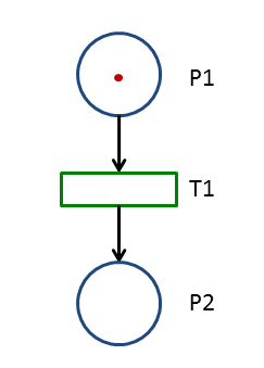
Figure 1: A simple Petri net

A place can hold tokens (in Figure 1, P1 holds one token as denoted by a red dot inside the circle), and an arc has its capacity (1 by default, otherwise the capacity is marked on the arc), and transitions have neither capacity, nor tokens. The marking (or state) of a Petri net is its token assignments of places. When the number of tokens in each input place is equal or larger than the arc weight (capacity), a transition is able to fire. When a transition fires, the tokens in input places are transferred to the output places, resulting in a new marking of the net. Figure 2 illustrates the firing of a transition, which reveals that the firing of a transition removes tokens from its input places and add tokens to its output places according to the capacity of the corresponding arcs. Note that tokens may disappear or appear going through a transition [Petri, 1966].

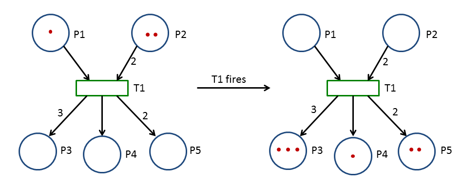
Figure 2: Firing of a transition

As the theory and methodology of Petri nets have been developed for more than 50 years, using Petri nets to model GRN will enrich our ability to analyse the dynamic properties of GRN. Several attempts have been made to model GRN using Petri nets [Chaouiya et al., 2004, Chaouiya et al., 2006, Chaouiya, 2007, Chaouiya et al., 2008, Liu and Heiner, 2014, Liu et al., 2017a, Liu et al., 2017d, Liu et al., 2017b, Liu et al., 2017c, Liu et al., 2018a, Liu and Chen, 2018, Liu et al., 2018b]. Here we adopt a simple model based on [Chaouiya et al., 2004, Dragan Bosnacki, 2004] and [Ruths et al., 2008]. In this model we draw an arrow from gene g2 to gene g1 to represent that g2 activates g1 (Figure 3a), and a blunt-end line from g2 to g1 will represent the inhibition of g1 by g2 (Figure 4a). For these two elementary GRNs we may construct the corresponding Petri nets, where genes are modelled as places, and the interaction between two genes is modelled by a transition together with directed arcs that connect the places and transitions.

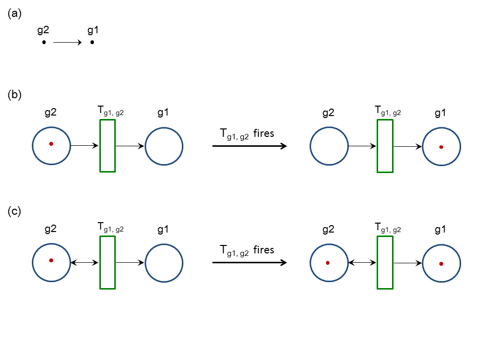
Figure 3: Activation of gene g1 by g2

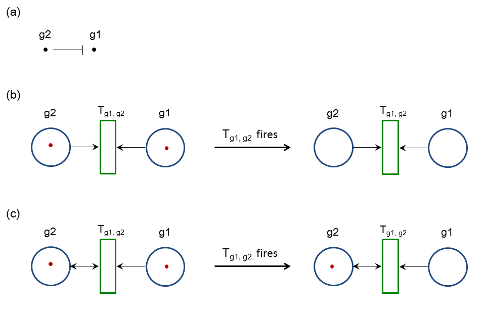
Figure 4: Inhibition of gene g1 by g2

In both activation and inhibition cases, g2 may or may not be consumed. We use double sided arrow to indicate that g2 activates g1 without itself being consumed (Figure 3c and 4c), and one sided arrow otherwise (Figure 3b and 4b). For activation, we draw an arrow pointing towards g1 from transition ${T_{g1,g2}}$, while for inhibition, we draw the arrow the other way round. Figure 3 and Figure 4 also describe what happens when ${T_{g1,g2}}$ fires. For example, in Figure 3b, before firing there is a token in g2 but none in g1, while after firing the token in g2 is consumed and g1 is activated as indicated by having a token in it.

Once we have these basic building blocks, we are able to convert a normal GRN into its corresponding Petri net. For example, if we have a GRN as shown in Figure 5a, then the Petri net for it will look like that in Figure 5b.

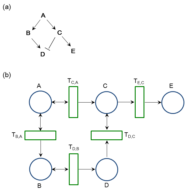
Figure 5: A simple GRN and its Petri net representation

Note that in this GRN gene A activates gene B and C, gene B activates gene D, and gene C inhibits gene D while activates gene E. Except in the case of C activating E, where C is consumed, all other transitions don’t consume the source gene.

Now that we obtain the Petri net modelling of a GRN, we shall be able to simulate and analyse the dynamics of the GRN [Ruths et al., 2008].

4 A Categorical Treatment of Petri nets

Unfortunately, standard Petri net lacks proper mechanisms for composition and abstraction, which makes it inadequate to model large or multi-scale GRN. The problem can be solved by viewing Petri net from the category theory perspective, i.e., treating Petri nets as monoids ([Meseguer and Montanari, 1990, Ermel and Martini, 1996]). In order to do that, we need to introduce two definitions, following Meseguer and Montanari’s work:

(1) A standard Petri net is a triple $<S,T,F>$, where S is a set of places, T is a set of transitions, and $F:(S\times T)+(T\times S)\rightarrow\mathbb{N}$ is a multiset which describes the connections between places and transitions. Here $\mathbb{N}$ represents natural numbers, $\times$ is the Cartesian product of sets, and + denotes the disjoint union of sets.

(2) A graph G is a set T of arcs, a set V of nodes and two functions $\partial_{0}$ and $\partial_{1}$ from T to V ($\partial_{0},\partial_{1}:T\rightarrow V$), called source and target, respectively. A graph morphism from G to G’ is a pair of functions $<f,g>,f:T\rightarrow T^{\prime},g:V\rightarrow V^{\prime}$ such that: $g\circ\partial_{0}=\partial_{0}^{\prime}\circ f$ and $g\circ\partial_{1}=\partial_{1}^{\prime}\circ f$.

In support of their motto ”Petri Nets Are Monoids”, Meseguer and Montanani argued that Petri nets can be viewed as ordinary, directed graphs equipped with parallel and sequential composition of transitions [Meseguer and Montanari, 1990]. Accordingly, they provided a new definition of Petri net:

A Petri net is a graph where the arcs in set are called transitions and where the set of nodes is the free commutative monoid $S^{\oplus}$ generated by the set of places S. The elements of $S^{\oplus}$ has the form $n_{1}a_{1}\oplus n_{2}a_{2}\oplus...n_{m}a_{m}$, where $a_{i}\in S,n_{i}\in\mathbb{N},i\in 1..m$, and m is the number of elements in S. The source and target functions go from T to $S^{\oplus}$ ($\partial_{0},\partial_{1}:T\rightarrow S^{\oplus}$). And a Petri net morphism $<f,g>$ is similar to a graph morphism, except that g is now a monoid homomorphism, which respects the monoid structure of $S^{\oplus}$.

This definition allows a different representation of the same standard Petri net. For example, if we have a Petri net $<S,T,F>$ as shown in Figure 6 where $S=\{g_{1},g_{2},g_{3}\}$, $T=\{t\}$, $F(g_{1},t)=1,F(g_{2},t)=1,F(t,g_{1})=1,F(t,g_{3})=1$, then we can represent it as $S^{\oplus}=\{g_{1},g_{2},g_{3}\}^{\oplus}$, $T=\{t\}$ and $\partial_{0}(t)=g_{1}+g_{2}$, $\partial_{1}(t)=g_{1}+g_{3}$.

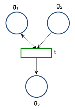
Figure 6: A simple GRN modelled in Petri net

Under such a representation, sequential and parallel compositions of Petri nets based on transitions could be obtained in a straightforward way. For example, a sequential composition of two Petri nets is illustrated in Figure 7, where the Petri net in Figure 7c is a composition of the Petri net in Figure 7b after that in Figure 7a.

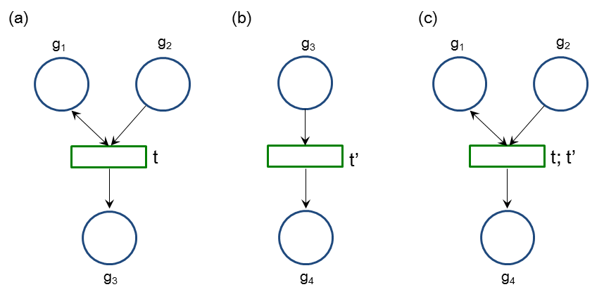
Figure 7: Sequential composition of Petri nets

On the other hand, a parallel composition of two Petri nets is shown in Figure 8, in which we calculate the products of places and transitions from Figure 8a and Figure 8b, and got the result Petri net in Figure 8c.

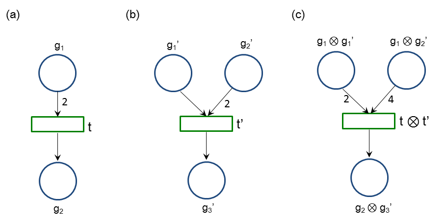
Figure 8: Parallel composition of Petri nets

With these two compositions at hands, we will be able to combine small Petri nets into large ones for the modelling of large GRNs.

Alternatively, we could construct the ”open” Petri net following Baez and Master’s recent work ([Baez and Master, 2018]).

The basic idea underlies an Open Petri net is that certain places in the Petri net are designated as inputs or outputs via a cospan of sets, which allows tokens to flow in or out of the Petri net and therefore make it open. From the categorical theory point of view, the input and output sets are objects and the open Petri net is the morphism between them, together they form a symmetric monoidal category ([Baez and Pollard, 2017, Baez and Master, 2018]). Further, in order to better describe vertical composition between sets and horizontal composition between open Petri nets, a symmetric monoidal double category $\mathbb{O}pen(Petri)$ was introduced. $\mathbb{O}pen(Petri)$ has the following components:
   (1) objects: sets X, Y, Z, …
   (2) vertical 1-morphisms: functions from set X to Y $(f:X\rightarrow Y)$
   (3) horizontal 1-cells: open Petri nets $(P:X\nrightarrow Y)$, which are cospans in Petri of the form:

here L is a functor from Set to Petri.

(4) 2-morphisms: morphisms between open Petri nets. A 2-morphism in $\mathbb{O}pen(Petri)$ has the following form:

We can compose 2-morphisms vertically by usual composition of functions as well as horizontally via the pushout of cospans. In addition, we can also obtain the tensor products of two 2-morphisms [Baez and Master, 2018]. For example, if we have two 2-morphisms as follows:

we can compose them vertically to get the 2-morphism:

And, for the following two 2-morphisms:

we can compose them horizontally to get the following 2-morphism:

Moreover, for the two 2-morphism like these:

we can calculate their tensor product to get the following 2-morphism:

5 Open Petri nets for gene regulatory networks

Finally, we will illustrate with an example on how to compose two GRNs (in the form of open Petri nets). The example presented here is based on that created in [Baez and Master, 2018]. Suppose we have the following two GRNs:

To compose them horizontal via pushout, we could first stick them side by side through the set Y and get the following intermediate network:

Then, we identify those places that are images of the same point in Y, group them together, and randomly choose one place to represent the group, removing set Y meanwhile [Baez and Master, 2018]. For example, point 2 in Y has images g3 and g6, so g3 and g6 are grouped together. Similarly, g4 and g6 are grouped together, and therefore we have g3, g4 and g6 all in the same group. Now we could merge those 3 places together, and we use g6 to represent this group. Also we merge g5 and g7 using g7 as representative place for them. We no longer need set Y and will obtain the composed open Petri net:

6 Conclusion and future work

In this preliminary work we attempt to model the gene regulatory networks (GRNs) with open Petri nets (OPNs) [Baez and Master, 2018]. OPN incorporates the power of both category theory and Petri nets, therefore it holds the great potential to become an ideal framework for systematic representation of GRNs. At this stage we only provide an example of how to compose two hypothetical GRNs written in the forms of OPNs. In the future we need to formalize on how to convert real GRNs into composable OPNs and further demonstrate that these OPN models facilitate the construction of large GRNs from smaller parts.

References

- [Baez and Fong, 2015] Baez, J. C. and Fong, B. (2015). A Compositional Framework for Passive Linear Networks.
- [Baez et al., 2015] Baez, J. C., Fong, B., and Pollard, B. S. (2015). A Compositional Framework for Markov Processes.
- [Baez and Master, 2018] Baez, J. C. and Master, J. (2018). Open Petri Nets.
- [Baez and Pollard, 2017] Baez, J. C. and Pollard, B. S. (2017). A Compositional Framework for Reaction Networks.
- [Baldan et al., 2015] Baldan, P., Bonchi, F., Gadducci, F., and Monreale, G. V. (2015). Modular encoding of synchronous and asynchronous interactions using open Petri nets. Science of Computer Programming, 109:96–124.
- [BALDAN et al., 2005] BALDAN, P., CORRADINI, A., EHRIG, H., and HECKEL, R. (2005). Compositional semantics for open Petri nets based on deterministic processes. Mathematical Structures in Computer Science, 15(1):1–35.
- [Bordon and Mraz, 2012] Bordon, J. and Mraz, M. (2012). Modeling gene regulatory networks using Petri Nets.
- [Chai et al., 2014] Chai, L. E., Loh, S. K., Low, S. T., Mohamad, M. S., Deris, S., and Zakaria, Z. (2014). A review on the computational approaches for gene regulatory network construction. Computers in Biology and Medicine, 48:55–65.
- [Chaouiya, 2007] Chaouiya, C. (2007). Petri net modelling of biological networks. Briefings in bioinformatics, 8(4):210–219.
- [Chaouiya et al., 2004] Chaouiya, C., Remy, E., Ruet, P., and Thieffry, D. (2004). Qualitative Modelling of Genetic Networks: From Logical Regulatory Graphs to Standard Petri Nets. pages 137–156. Springer, Berlin, Heidelberg.
- [Chaouiya et al., 2006] Chaouiya, C., Remy, E., and Thieffry, D. (2006). Qualitative Petri Net Modelling of Genetic Networks. pages 95–112. Springer, Berlin, Heidelberg.
- [Chaouiya et al., 2008] Chaouiya, C., Remy, E., and Thieffry, D. (2008). Petri net modelling of biological regulatory networks. Journal of Discrete Algorithms, 6(2):165–177.
- [de Jong, 2002] de Jong, H. (2002). Modeling and Simulation of Genetic Regulatory Systems: A Literature Review. Journal of Computational Biology, 9(1):67–103.
- [Delgado and Gómez-Vela, 2018] Delgado, F. M. and Gómez-Vela, F. (2018). Computational methods for Gene Regulatory Networks reconstruction and analysis: A review. Artificial Intelligence in Medicine, 95:133–145.
- [Dragan Bosnacki, 2004] Dragan Bosnacki (2004). Modeling of Genetic Networks with Petri Nets. Technical report.
- [Ermel and Martini, 1996] Ermel, C. and Martini, A. (1996). A Taste of Categorical Petri Nets. Technical report.
- [Hamed, 2018] Hamed, R. I. (2018). Quantitative modeling of gene networks of biological systems using fuzzy Petri nets and fuzzy sets. Journal of King Saud University - Science, 30(1):112–119.
- [Liu and Chen, 2018] Liu, F. and Chen, S. (2018). Colored Fuzzy Petri Nets for Dealing with Genetic Regulatory Networks. Fundamenta Informaticae, 160(1-2):101–118.
- [Liu and Heiner, 2014] Liu, F. and Heiner, M. (2014). Petri Nets for Modeling and Analyzing Biochemical Reaction Networks. In Approaches in Integrative Bioinformatics, pages 245–272. Springer Berlin Heidelberg, Berlin, Heidelberg.
- [Liu et al., 2017a] Liu, F., Heiner, M., and Gilbert, D. (2017a). Coloured Petri nets for multilevel, multiscale and multidimensional modelling of biological systems. Briefings in Bioinformatics.
- [Liu et al., 2017b] Liu, F., Heiner, M., and Gilbert, D. (2017b). Coloured Petri nets for multilevel, multiscale and multidimensional modelling of biological systems. Briefings in Bioinformatics.
- [Liu et al., 2017c] Liu, F., Heiner, M., and Gilbert, D. (2017c). Coloured Petri nets for multilevel, multiscale and multidimensional modelling of biological systems. Briefings in Bioinformatics.
- [Liu et al., 2018a] Liu, F., Heiner, M., and Gilbert, D. (2018a). Fuzzy Petri nets for modelling of uncertain biological systems. Briefings in Bioinformatics.
- [Liu et al., 2018b] Liu, F., Heiner, M., and Gilbert, D. (2018b). Fuzzy Petri nets for modelling of uncertain biological systems. Briefings in Bioinformatics.
- [Liu et al., 2017d] Liu, H.-C., You, J.-X., Li, Z., and Tian, G. (2017d). Fuzzy Petri nets for knowledge representation and reasoning: A literature review. Engineering Applications of Artificial Intelligence, 60:45–56.
- [Meseguer and Montanari, 1990] Meseguer, J. and Montanari, U. (1990). Petri nets are monoids. Information and Computation, 88(2):105–155.
- [Murata, 1989] Murata, T. (1989). Petri nets: Properties, analysis and applications. Proceedings of the IEEE, 77(4):541–580.
- [Petri, 1962] Petri, C. A. (1962). Kommunikation mit automaten.
- [Petri, 1966] Petri, C. A. (1966). Communication with automata.
- [Rathke et al., 2014] Rathke, J., Soboci´nski, S., and Stephens, O. (2014). Compositional Reachability in Petri Nets. In International Work- shop on Reachability Problems, Lecture Notes in Computer Science 8762, Springer, Berlin, 2014.
- [Reisig, 1985] Reisig, W. (1985). Petri Nets : an Introduction. Springer Berlin Heidelberg.
- [Ruths et al., 2008] Ruths, D., Muller, M., Tseng, J.-T., Nakhleh, L., and Ram, P. T. (2008). The Signaling Petri Net-Based Simulator: A Non-Parametric Strategy for Characterizing the Dynamics of Cell-Specific Signaling Networks. PLoS Computational Biology, 4(2):e1000005.
- [Steggles et al., 2007] Steggles, L. J., Banks, R., Shaw, O., and Wipat, A. (2007). Qualitatively modelling and analysing genetic regulatory networks: a Petri net approach. Bioinformatics, 23(3):336–343.