DEAM: Adaptive Momentum with Discriminative Weight for Stochastic Optimization

Abstract

Optimization algorithms with momentum, e.g., (ADAM), have been widely used for building deep learning models due to the faster convergence rates compared with stochastic gradient descent (SGD). Momentum helps accelerate SGD in the relevant directions in parameter updating, which can minify the oscillations of parameters update route. However, there exist errors in some update steps in optimization algorithms with momentum like ADAM. The fixed momentum weight (e.g., $\beta_{1}$ in ADAM) will propagate errors in momentum computing. In this paper, we introduce a novel optimization algorithm, namely Discriminative wEight on Adaptive Momentum (DEAM). Instead of assigning the momentum term weight with a fixed hyperparameter, DEAM proposes to compute the momentum weight automatically based on the discriminative angle. In this way, DEAM involves fewer hyperparameters. DEAM also contains a novel backtrack term, which restricts redundant updates when the correction of the last step is needed. Extensive experiments demonstrate that DEAM can achieve a faster convergence rate than the existing optimization algorithms in training the deep learning models of both convex and non-convex situations.

1 Introduction

Deep learning methods can achieve outstanding performance in multiple fields including computer vision He et al. (2016), natural language processing Dong et al. (2015); Bahdanau et al. (2014), speech and audio processing Neumann and Vu (2017), and graph analysis Zhang (2019). Training deep learning models involves an optimization process to find the parameters in the model that minimize the loss function. At the same time, the number of parameters commonly used in deep learning methods can be very huge.

Therefore, optimization algorithms are critical for deep learning methods: not only the model performance, but also training efficiency are greatly affected. In order to cope with the high computational complexity of training deep learning methods, stochastic gradient descent (SGD) Ruder (2017) is utilized to update parameters based on the gradient of each training sample instead. The idea of momentum Qian (1999), inspired by Newton’s first law of motion, is used to handle the oscillations of SGD. SGD with momentum Sutskever et al. (2013b) achieves the faster convergence rate and better optimization results compared with the original SGD. In gradient descent based optimization, training efficiency is also greatly affected by the learning rate. AdaGrad Duchi et al. (2011) is the first optimization algorithm with adaptive learning rates, which makes use of the learning rate decay. AdaDelta Zeiler (2012) subsequently improves AdaGrad to avoid the extremely small learning rates. ADAM Kingma and Ba (2015) involves both adaptive learning Ruder (2017) and momentum Qian (1999) and utilizes the exponential decay rate $\beta_{1}$ (momentum weight) to accelerate the convergence in the relevant directions and dampen oscillations. However, the decay rate $\beta_{1}$ of the first-order momentum $\mathbf{m}_{t}$ in ADAM is a fixed number, and the selection of the hyperparameter $\beta_{1}$ may affect the performance of ADAM greatly. Commonly, $\beta_{1}=0.9$ is the most widely used parameter as introduced in Kingma and Ba (2015), but there is still no theoretical evidence proving its advantages.

During the optimization process, it is common that there exist errors in some update steps. These errors can be caused by the inappropriate momentum calculation, and then lead to slower convergence or oscillations. For each parameter updates, using the fixed momentum weight fails to take the different influence of the current gradient into consideration, which will render errors in momentum computing. For example, when there exist parts of opposite eigen components Qian (1999) between the continuous two parameter updates (we regard this situation as an error), the current gradient should be assigned a larger weight to correct the momentum in the last update, instead of being placed with a fixed influence. We will illustrate this problem through cases in Section 3.1.1 where ADAM with a fixed weight $\beta_{1}$ cannot handle some simple but intuitive convex optimization problems. Based on this situation, we need to control the influence of momentum by an adaptive weight. What’s more, designing hyperparameter-free optimization algorithms has been a very important research problem in recent years, controlling the number of hyperparameters will not only stabilize the performance of the optimization algorithm, but also release the workload of hyperparameters tuning.

In this paper, we introduce a novel optimization algorithm, namely DEAM (Discriminative wEight on Adaptive Momentum) to deal with the aforementioned problems. DEAM proposes an adaptive momentum weight $\beta_{1,t}$, which will be learned and updated in each training iteration automatically. Besides, DEAM employs a novel backtrack term $d_{t}$, which will restrict redundant updates when DEAM decides that the correction of the previous step is needed. We also provide the theoretic analyses about the adaptive momentum weight along with extensive experiments. Based on them, we verify that the adaptive momentum term weight $\beta_{1,t}$ and the operation of backtrack term $d_{t}$ can be crucial for the performance of the learning algorithms.

Here, we summarize the detailed learning mechanism of DEAM as follows:

• DEAM computes adaptive momentum weight $\beta_{1,t}$ based on the “discriminative angle” $\theta$ between the historical momentum and the newly calculated gradient.

• DEAM introduces a novel backtrack term, i.e., $d_{t}$, which is proposed to correct the redundant update of the previous training epoch if it is necessary. The calculation of $d_{t}$ is also based on the discriminative angle $\theta$.

• DEAM involves fewer hyperparameters than the ADAM during the training process, which can decrease the workload of hyperparameter tuning.

Detailed information about the learning mechanism and the concepts mentioned above will be described in the following sections. This paper will be organized as follows. In Section 2, we will cover some related works about widely used optimization algorithms. In Section 3, we will analyze more detail of our proposed algorithm, whose theoretic convergence rate will also be studied. Extensive experiments will be exhibited in Section 4. Finally, we will give a conclusion of this paper in Section 5.

2 Related Works

Stochastic Gradient Descent: Stochastic gradient descent (SGD) Ruder (2017); Bianchi and Jakubowicz (2012) performs parameter updating for each training example and label. The advantages of SGD include fast converging speed compared with gradient descent and preventing redundancy Ruder (2017). Reddi et al. (2015) use the variance reduction methods to accelerate the training process of SGD.

Adaptive Learning Rates: To overcome the problems brought by the unified learning rate, some variant algorithms applying adaptive learning rate Behera et al. (2006) have been proposed, such as AdaGrad Duchi et al. (2011), AdaDelta Zeiler (2012), RMSProp Tieleman and Hinton (2012), ADAM Kingma and Ba (2015) and recent ESGD Dauphin et al. (2015), AdaBound Luo et al. (2019). AdaGrad adopts different learning rates to different variables. One drawback of AdaGrad is that with the increasing of iteration number $t$, the adaptive term may inflate continuously, which leads to a very slow convergence rate in the later stage of the training process. RMSProp can solve this problem by using the moving average of historical gradients.

Momentum: Momentum Qian (1999); Sutskever et al. (2013a); Li et al. (2017); Dozat (2016); Mitliagkas et al. (2016) is a method that helps accelerate SGD in the relevant direction and prevent oscillations on the descent route. The momentum accelerates updates for dimensions whose gradients are in the same direction as historical gradients, and decelerates updates for dimensions whose gradients are the opposite. Momentum is also applied to Nesterov accelerated gradient (NAG) Nesterov (1983), which provides the momentum term with the estimating next position capability. Instead of using the current location to calculate the gradient, NAG first approximates the next position of the variables, then uses the approximated future position to compute the gradient. ADAM Kingma and Ba (2015); Zhang et al. (2018) is proposed based on momentum and adaptive learning rates for different variables. ADAM records the first-order momentum and the second-order momentum of the gradients using the moving average, and further computes the bias-corrected version of them. Based on ADAM, Keskar et al. Keskar and Socher (2017) proposes to switch from ADAM to SGD during the training process. AMSGrad Reddi et al. (2018) is a modified version of ADAM, which redefines second-order momentum by a maximum function.

3 Proposed Algorithm

Our proposed algorithm DEAM is presented in Algorithm 1. In the algorithm, $f_{1},f_{2},\dots,f_{T}$ is a sequence of loss functions computed with the training mini-batches in different iterations (or epochs).

Algorithm 1 DEAM Algorithm

Input: loss function $f(\mathbf{w})$ with parameters $\mathbf{w}$; learning rate $\{\eta_{t}\}^{T}_{t=1}$; $\beta_{2}=0.999$
  Output: trained parameters

1:$\mathbf{m}_{0}\leftarrow\mathbf{0}$ /* Initialize first-order momentum */

2:$\mathbf{v}_{0}\leftarrow\mathbf{0}$, $\mathbf{\hat{v}}_{0}\leftarrow\mathbf{0}$ /* Initialize second-order momentum */

3:for $t=1,2,\dots,T$ do

4:    $\mathbf{g}_{t}=\nabla f_{t}(\mathbf{w}_{t})$,

5:    $\theta=\left\langle\frac{\mathbf{m}_{t-1}}{\sqrt{\mathbf{\hat{v}}_{t-1}}},\mathbf{g}_{t}\right\rangle$  /* The operator $\left\langle\cdot,\cdot\right\rangle$ represents the angle between two vectors. */

6:    if $\theta\in[0,\frac{\pi}{2})$ then

7:        $\beta_{1,t}=\sin\theta/K+\epsilon$

8:    else

9:        $\beta_{1,t}=1/K$  /* Here, $K=\frac{10(2+\pi)}{2\pi}$. */

10:    end if

11:    $\mathbf{m}_{t}=(1-\beta_{1,t})\cdot\mathbf{m}_{t-1}+\beta_{1,t}\cdot\mathbf{g}_{t}$

12:    $\mathbf{v}_{t}=\beta_{2}\cdot\mathbf{v}_{t-1}+(1-\beta_{2})\cdot\mathbf{g}_{t}\odot\mathbf{g}_{t}$ /* $\odot$ is element-wise multiplication.*/

13:    $\mathbf{\hat{v}}_{t}=\max\{\mathbf{\hat{v}}_{t-1},\mathbf{v}_{t}\}$

14:    $d_{t}=\min\{0.5\cos\theta,0\}$

15:    $\mathbf{\Delta}_{t}=d_{t}\cdot\mathbf{\Delta}_{t-1}-\eta_{t}\cdot\frac{\mathbf{m}_{t}}{\sqrt{\mathbf{\hat{v}}_{t}}}$

16:    $\mathbf{w}_{t}=\mathbf{w}_{t-1}+\mathbf{\Delta}_{t}$

17:end for

18:return $\mathbf{w}_{T}$

DEAM introduces two new terms in the learning process: (1) the adaptive momentum weight $\beta_{1,t}$, and (2) the“backtrack term” $d_{t}$. In the $t_{th}$ training iteration, both $\beta_{1,t}$ and $d_{t}$ are calculated based on the “discriminative angle” $\theta$, which is the angle between previous $\mathbf{m}_{t-1}/\sqrt{\mathbf{\hat{v}}_{t-1}}$ and current gradient $\mathbf{g}_{t}$ (since essentially both $\mathbf{m}_{t-1}/\sqrt{\mathbf{\hat{v}}_{t-1}}$ and $\mathbf{g}_{t}$ are vectors, there exists an angle between them). Here, $\mathbf{m}$ is the first-order momentum that records the exponential moving average of historical gradients; $\mathbf{v}$ is the exponential moving average of the squared gradients, which is called the second-order momentum. In the following parts of this paper, we will denote $\mathbf{m}_{t-1}/\sqrt{\mathbf{\hat{v}}_{t-1}}$ as the “update volume” in the ${(t-1)}_{th}$ iteration. Formally, $\beta_{1,t}$ determines the weights of previous first-order momentum $\mathbf{m}_{t-1}$ and current gradient $\mathbf{g}_{t}$ when calculation the present $\mathbf{m}_{t}$. Meanwhile, the backtrack term $d_{t}$ represents the returning step of the previous update on parameters. We can notice that in each iteration, after the $\theta$ has been calculated, the $\beta_{1,t}$ and $d_{t}$ are directly obtained according to the $\theta$. In this way, we can calculate appropriate $\beta_{1,t}$ as the discriminative angle changes. The $d_{t}$ term balances between the historical update term $\mathbf{\Delta}_{t-1}$ (defiend in Algorithm 1) and the current update volume $\mathbf{m}_{t}/\sqrt{\mathbf{\hat{v}}_{t}}$ when computing $\mathbf{\Delta}_{t}$. In the proposed DEAM, $\beta_{1,t}$ and $d_{t}$ terms can collaborate with each other and achieve faster convergence.

3.1 Adaptive Momentum Weight $\beta_{1,t}$

3.1.1 Motivation

In the ADAM Kingma and Ba (2015) paper, (the first-order) momentum’s weight (i.e., $\beta_{1}$) is a pre-specified fixed value, and commonly $\beta_{1}=0.9$. It has been used in many applications and the performance can usually meet the expectations. However, this setting is not applicable in some situations. For example, for the case

$$f(x,y)=x^{2}+4y^{2},$$ (1)

where $x$ and $y$ are two variables, it is obvious that $f$ is a convex function. If $f(x,y)$ is the objective function to optimize, we try to use ADAM to find its global optima.

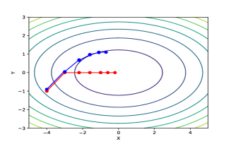
Figure 1: The update routes of ADAM with $\beta_{1}=0.9$ (the blue line) and $\beta_{1}=0.0$ (the red line).

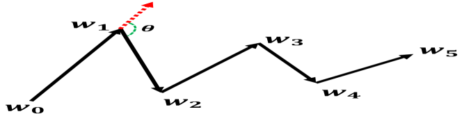
(a) The ”zig-zag” route

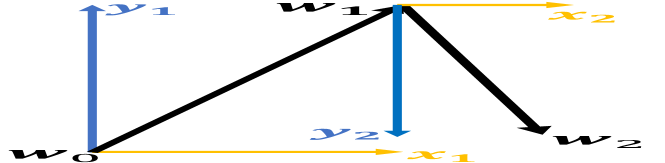
(b) Axis decomposition

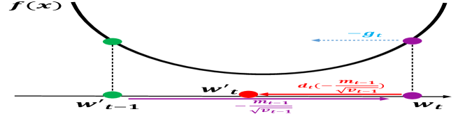
(c) Example: When $\theta=180^{\circ}$

Figure 2: Some examples about $d_{t}$

Let’s assume ADAM starts the variable search from $(-4,-1)$ (i.e., the initial variable vector is $\mathbf{w}_{0}=(-4,-1)^{\top}$) and the initial learning rate is $\eta_{1}=1$. Different choices of $\beta_{1}$ will lead to very different performance of ADAM. For instance, in Figure 1, we illustrate the update routes of ADAM with $\beta_{1}=0.9$ and $\beta_{1}=0.0$ as the blue and red lines, respectively. In Figure 1, the ellipse lines are the contour lines of $f(x,y)$, and points on the same line share the same function value. We can observe that after the first updating, both of the two approaches will update variables to $(-3,0)$ point (i.e., the updated variable vector will be $\mathbf{w}_{1}=(-3,0)^{\top}$). In the second step, since the current gradient $\mathbf{g}_{2}=(-6,0)^{\top}$, the ADAM with $\beta_{1}=0.0$ will update variables in the $(1,0)$ direction. Meanwhile, for the ADAM with $\beta_{1}=0.9$, its $\mathbf{m}_{2}$ is computed by integrating $\mathbf{m}_{1}$ and $\mathbf{g}_{2}$ together (whose weights are $\beta_{1}$ and $1-\beta_{1}$, respectively). Therefore the updating direction of it will be more inclined to the previous direction instead. Compared with ADAM with $\beta_{1}=0.0$, the ADAM with $\beta_{1}=0.9$ takes much more iterations until converging.

From the analysis above, we can observe that, a careful tuning and updating of $\beta_{1}$ in the learning process can be crucial for the performance of ADAM. However, by this context so far, there still exist no effective approaches for guiding the parameter tuning yet. To deal with this problem, DEAM introduces the concept of discriminative angle $\theta$ for computing $\beta_{1}$ automatically as follows.

3.1.2 Mechanism

The momentum weight $\beta_{1}$ will be updated in each iteration in DEAM, and we can denote its value computed in the $t_{th}$ iteration as $\beta_{1,t}$ formally. Essentially, in the $t_{th}$ iteration of the training process, both the previous update volume and $\mathbf{g}_{t}$ are vectors (or directions), and these directions directly decide the updating process. Thus we try to extract their relation with the help of angle, and subsequently determine the weight $\beta_{1,t}$ (or $1-\beta_{1,t}$) by the angle.

In Algorithm 1, the discriminative angle $\theta$ in the $t_{th}$ iteration is calculated by

$$\theta=\left\langle-\frac{\mathbf{m}_{t-1}}{\sqrt{\mathbf{\hat{v}}_{t-1}}},-\mathbf{g}_{t}\right\rangle=\left\langle\frac{\mathbf{m}_{t-1}}{\sqrt{\mathbf{\hat{v}}_{t-1}}},\mathbf{g}_{t}\right\rangle$$ (2)

Here, the operator $\left\langle\cdot,\cdot\right\rangle$ denotes the angle between two vectors. This expression is easy to understand, since the $-\mathbf{m}_{t-1}/\sqrt{\mathbf{\hat{v}}_{t-1}}$ can represent the updating direction of $(t-1)_{th}$ iteration in AMSGrad, meanwhile $-\mathbf{g}_{t}$ is the reverse of the present gradient. So we can simplify it as $\theta=<\frac{\mathbf{m}_{t-1}}{\sqrt{\mathbf{\hat{v}}_{t-1}}},\mathbf{g}_{t}>$. If $\theta$ is close to zero (denoted by $\theta\rightarrow 0^{\circ}$), the $\mathbf{m}_{t-1}/\sqrt{\mathbf{\hat{v}}_{t-1}}$ (previous update volume) and $\mathbf{g}_{t}$ are almost in the same direction, and the weights for them will not be very important. Meanwhile, if $\theta$ approaches $180^{\circ}$ (denoted by $\theta\rightarrow 180^{\circ}$), the previous update volume and $\mathbf{g}_{t}$ will be in totally reverse directions. This means in the current step, the previous momentum term is already in a wrong direction. Therefore, to rectify this error of the last momentum, DEAM proposes to assign the current gradient’s weight (i.e., $\beta_{1,t}$ in our paper) with a larger value instead. As the $\beta_{1,t}$ varies when $\theta$ changes from $0^{\circ}$ to $180^{\circ}$, we intend to define $\beta_{1,t}$ with the following equation:

$$\beta_{1,t}=\begin{cases}\sin\ K+\epsilon&\mbox{$\theta\in[0,\frac{\pi}{2})$}\\ 1/K&\mbox{$\theta\in[\frac{\pi}{2},\pi]$}\end{cases}$$ (3)

where $K=10(2+\pi)/2\pi$ and $\epsilon$ is a very small value (e.g., $\epsilon=0.001$). In the equation above, the threshold of the piecewise function is $\theta=\pi/2$, because $\sin\theta$ comes to the maximum at this point and goes down when $\theta>\frac{\pi}{2}$. If $\frac{\pi}{2}\leq\theta\leq\pi$, which is exactly the situation $\theta\rightarrow 180^{\circ}$ we discussed above, we intend to keep $\beta_{1,t}$ in a relatively large value. The reason we rescale $\sin\theta$ by ${1}/{K}$ is that directly applying $\beta_{1,t}=\sin\theta$ will overweight $\mathbf{g}_{t}$, which may cause fluctuations on the update routes. The value of $K$ is determined by:

$$K=10(\int_{0}^{\frac{\pi}{2}}\sin\theta d\theta+\int_{\frac{\pi}{2}}^{\pi}1d\theta)=\frac{10(2+\pi)}{2\pi}$$ (4)

In the equation above, assume $\theta$ is randomly distributed on $[0,\pi]$, in this calculation we can get

$$\mathbb{E}[\beta_{1,t}]=\frac{1}{\pi}\int_{0}^{\pi}\beta_{1,t}(\theta)d\theta=0.1$$ (5)

In other words, the expectation of $\beta_{1,t}$ (i.e., $\mathbb{E}(\beta_{1,t})$) will be identical to the $\beta_{1}$ used in ADAM Kingma and Ba (2015). After obtaining $\beta_{1,t}$, it will be applied to calculating $\mathbf{m}_{t}$ as shown in Algorithm 1. In this way, we have achieved momentum with adaptive weights, and this weight is automatically computed during the training process, fewer hyperparameters will be involved.

3.2 Backtrack Term $d_{t}$

To further speed up the convergence rate, we employ a novel backtrack mechanism for DEAM. As a mechanism computed based on the discriminative angle $\theta$, the backtrack term allows DEAM to eliminate redundant update in each iteration. Besides, according to our following analysis, the backtrack term $d_{t}$ virtually collaborates with the $\beta_{1,t}$ term to further accelerate the convergence of the training process.

3.2.1 Motivation

When optimizer (e.g., ADAM) updates variables of the loss function (e.g., $f(x,y)$), some update routes will look like the black arrow lines shown in Figure 2(a), especially when the discriminative angle $\theta$ is larger than $90^{\circ}$. We call this phenomenon the ”zig-zag” route. In Figure 2(a), it shows the update routes of a 2-dimension function. Each black arrow line in the figure represents the variables’ update in each epoch; the red dashed line is the direction of the update routes; the $\theta$ is the discriminative angle. If $\theta\geq 90^{\circ}$, the ”zig-zag” phenomenon will appear severely, which may lead to slower convergence speed. The main reason is when $\theta\geq 90^{\circ}$, if we map two neighboring update directions onto the coordinate axes, there will be at least one axis of the directions being opposite. This situation is shown in Figure 2(b). For the example of a function with 2-dimension variables, the update volume $\mathbf{m}_{1}/\sqrt{\mathbf{v}_{1}}$ can be decomposed into $(x_{1},y_{1})^{\top}$ in Figure 2(b), and the same with $\mathbf{m}_{2}/\sqrt{\mathbf{v}_{2}}$. We can notice that $y_{1}$ and $y_{2}$ are in the opposite directions, so the first and second steps practically have inverse updates subject to the $y$ axis. We attribute this situation to the over update (or redundant update) of the first step. Therefore the backtrack term $d_{t}$ is proposed to restrict this situation.

3.2.2 Mechanism

Since the redundant update situation is caused by over updating of the previous iteration, simply we intend to deal with it through a backward step. Meanwhile, during the updating process of variables, not every step will suffer from the redundant update: if $\theta\rightarrow 0^{\circ}$, the updating process becomes smooth, not like the situation shown in Figure 2(a). Besides, from the analysis above we conclude that if $\theta\geq 90^{\circ}$, there will be at least one dimension involves the redundant update. Thus, in the $t_{th}$ iteration we quantify $d_{t}$ as the following equation:

$$d_{t}=\min\{0.5\cos\theta,0\}$$ (6)

and we rewrite the updating term with backtrack in DEAM as

$$\mathbf{\Delta}_{t}=d_{t}\cdot\mathbf{\Delta}_{t-1}-\eta_{t}\cdot\frac{\mathbf{m}_{t}}{\sqrt{\mathbf{\hat{v}}_{t}}}$$ (7)

where $\theta$ is the discriminative angle and $\mathbf{\Delta}_{t}$ is the updating term in Algorithm 1. By designing $d_{t}$ in this way, when $\theta\rightarrow 0^{\circ}$, $d_{t}=0$ and there is no backward step, the updating term $\mathbf{\Delta}_{t}=-\eta_{t}\cdot\frac{\mathbf{m}_{t}}{\sqrt{\mathbf{\hat{v}}_{t}}}$ is similar to AMSGrad; when $\theta\rightarrow 180^{\circ}$, $d_{t}=0.5\cos\theta$ and comes to the maximum value when $\theta=180^{\circ}$. The reason that $\cos\theta$ is rescaled by $0.5$ is that: in Figure 2(c), $\mathbf{w}_{t-1}$ and $\mathbf{w}_{t}$ are the variables updated by DEAM without $d_{t}$ term in the $(t-1)_{th}$ and $t_{th}$ iterations respectively. If the backtrack mechanism is implemented, in the $(t+1)_{th}$ iteration, since $\theta=180^{\circ}$, firstly $d_{t}=0.5\cos\theta\to-0.5$ makes the backtrack to the $\mathbf{w^{\prime}}_{t}$ point (the middle point of $\mathbf{w}_{t-1}$ and $\mathbf{w}_{t}$). Thus, this backtrack step allows the variable to further approach the optima.

By implementing the backtrack term $d_{t}$, DEAM can combine it with the adaptive momentum weight $\beta_{1,t}$ to achieve the collaborating of them. For the situation of large discriminative angle ($\theta>90^{\circ}$), both $\beta_{1,t}$ and $d_{t}$ in the current step can make corrections to the last update. Since when $\theta>90^{\circ}$, the last update is in conflict direction compared with the current gradient, and $\beta_{1,t}$ will increase to allocate a large weight for the present gradient, which subsequently corrects the previous step. Meanwhile, the $d_{t}$ will also conduct a backward step of to further rectify the last update.

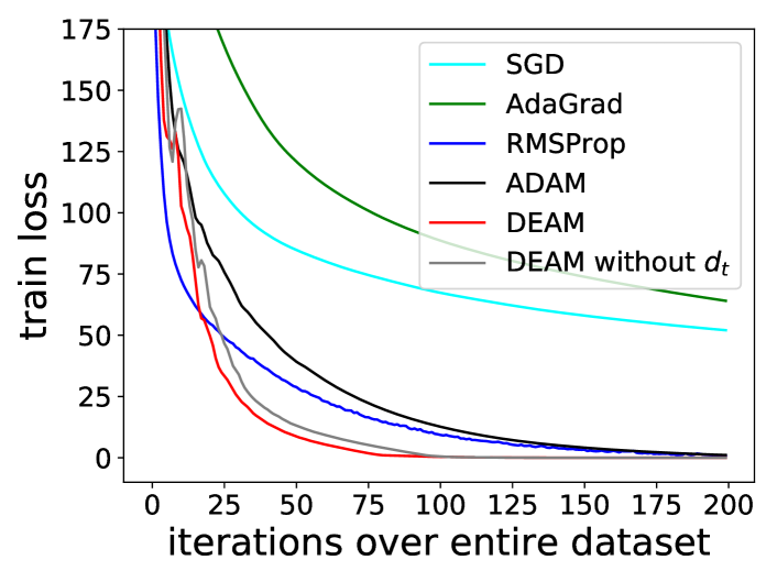
(a) Train loss on ORL

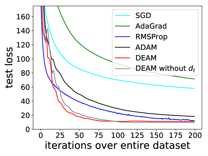
(b) Test loss on ORL

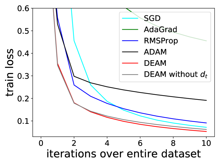
(c) Train loss on MNIST

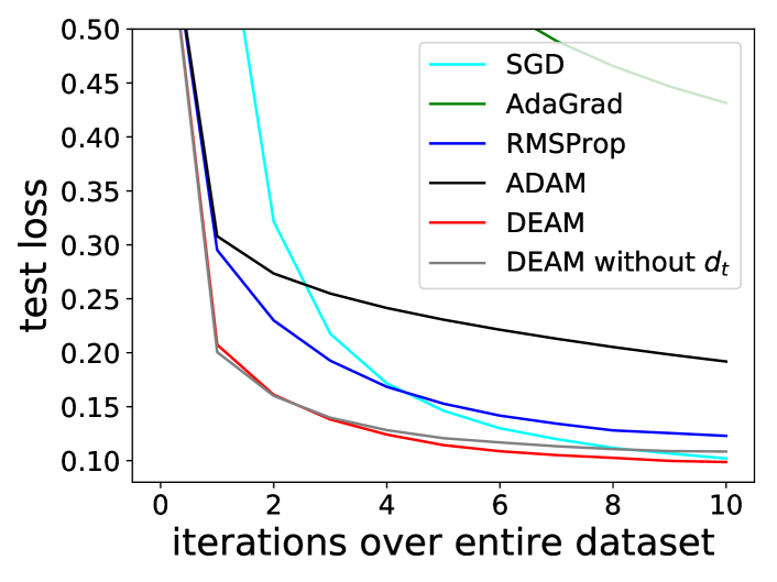
(d) Test loss on MNIST

Figure 3: Results of Logistic Regression and DNN structures

3.3 Theoretical Analysis

In this part, we give the detailed analysis on the convergence of our DEAM algorithm. According to Kingma and Ba (2015); Reddi et al. (2018); Zinkevich (2003); Chen et al. (2019), given an arbitrary sequence of convex objective functions $f_{1}(\mathbf{w}),f_{2}(\mathbf{w}),\dots,f_{T}(\mathbf{w})$, we intend to evaluate our algorithm using the regret function, which is denoted as:

$$R(T)=\sum_{t=1}^{T}[f_{t}(\mathbf{w}_{t})-f_{t}(\mathbf{w}^{*})]$$ (8)

where $\mathbf{w}^{*}$ is the globally optimal point. In the following Theorem 1, we will show that the above regret function is bounded. Before proving the Theorem 1, there are some definitions and lemmas as the pre-requisites.

Definition 1.

If a function $f:\mathbb{R}^{d}\rightarrow\mathbb{R}$ is convex, then $\forall x,y\in\mathbb{R}^{d}$, $\forall\phi\in[0,1]$, we have

$$f(\phi x+(1-\phi)y)\leq\phi f(x)+(1-\phi)f(y)$$

Definition 2.

If a function $f:\mathbb{R}^{d}\rightarrow\mathbb{R}$ is convex, then $\forall x,y\in\mathbb{R}^{d}$ we have

$$f(y)\geq f(x)+\nabla f(x)^{\top}(y-x)$$

Lemma 1.

Assume that the function $f_{t}$ has bounded gradients, $\left\|\nabla f_{t}(\mathbf{w})\right\|_{\infty}\leq G_{\infty}$. Let $\mathbf{m}_{t,i}$ represents the $i_{th}$ element of $\mathbf{m}_{t}$ in DEAM, then the $\mathbf{m}_{t,i}$ is bounded by

$$\mathbf{m}_{t,i}\leq\frac{(1-\epsilon_{0})G_{\infty}}{K(1-\lambda)}$$

Proof.

Let $g_{t}=\nabla f_{t}(\mathbf{w})$. According to the definition of $\mathbf{m}_{t,i}$ in our algorithm,

$$\mathbf{\mathbf{m}}_{t,i} =\sum_{j=1}^{t}\beta_{1,j}\prod_{l=1}^{t-j}(1-\beta_{1,t-l+1})g_{j,i}$$

$$\leq\frac{G_{\infty}}{K}\sum_{j=1}^{t}\prod_{l=1}^{t-j}(1-\epsilon)\leq\frac{G_{\infty}}{K}\sum_{j=1}^{t}(1-\epsilon_{0})\lambda^{t-j}\leq\frac{(1-\epsilon_{0})G_{\infty}}{K(1-\lambda)}$$

where $K$ and $\epsilon$ are the terms in Algorithm 1. ∎

For the following proof, $\mathbf{g}_{t}:=\nabla f_{t}(\mathbf{w}_{t})$ and $\mathbf{g}_{t,i}$ will represent the $i_{th}$ element of $\mathbf{g}_{t}\in\mathbb{R}^{d}$, and $\mathbf{g}_{1:t,i}=[\mathbf{g}_{1,i},\mathbf{g}_{2,i},\dots,\mathbf{g}_{t,i}]$.

Theorem 1.

Assume $\{f_{t}\}_{t=1}^{T}$ have bounded gradients $\left\|\nabla f_{t}(\mathbf{w})\right\|_{\infty}\leq G_{\infty}$ for all $\mathbf{w}\in\mathbb{R}^{d}$, all variables are bounded by $\left\|\mathbf{w}_{p}-\mathbf{w}_{q}\right\|_{2}\leq D$ and $\left\|\mathbf{w}_{p}-\mathbf{w}_{q}\right\|_{\infty}\leq D_{\infty}$, $\forall p,q\in\{1,2,\dots,T\}$, $\eta_{t}=\eta/\sqrt{t}$, $\gamma_{1}=(1-\epsilon_{0})/\sqrt{\beta_{2}}$ and satisfies $\gamma_{1}<1$, $\epsilon=1-(1-\epsilon_{0})\lambda^{t-1},\lambda\in(0,1)$. Our proposed algorithm can achieve the following bound on regret:

$$R(t) \leq\frac{D^{2}}{\epsilon_{0}\eta}\sum_{i=1}^{d}\sqrt{T\mathbf{\hat{v}}_{T,i}}+\frac{(1-\epsilon_{0})^{2}G_{\infty}D_{\infty}d}{K(1-\lambda)^{2}\epsilon_{0}}$$

$$+\frac{\eta\sqrt{1+\log T}}{2\epsilon^{2}_{0}(1-\gamma_{1})\sqrt{1-\beta_{2}}}\sum_{i=1}^{d}\left\|\mathbf{g}_{1:T,i}\right\|_{2}$$

Proof.

According to Definition 2, for $\forall t\in\{1,2,\dots,T\}$, we have

$$f_{t}(\mathbf{w}_{t})-f_{t}(\mathbf{w}^{*})\leq\nabla f_{t}(\mathbf{w}_{t})^{\top}(\mathbf{w}_{t}-\mathbf{w}^{*})=\sum_{i=1}^{d}\mathbf{g}_{t,i}(\mathbf{w}_{t,i}-\mathbf{w}_{i}^{*})$$

From the definition of $\mathbf{\Delta}_{t}$ in the updating rule of DEAM, we know it is equal to multiplying the learning rate $\eta_{t}$ in some iterations by a number in $[0.5,1]$, which means $\mathbf{w}_{t+1}=\mathbf{w}_{t}-\hat{\eta}_{t}\cdot\frac{\mathbf{m}_{t}}{\sqrt{\mathbf{\hat{v}}_{t}}};\hat{\eta}_{t}=\mu_{t}\cdot\eta_{t}$, where $\mu_{t}\in[0.5,1]$. If we first focus on the $i_{th}$ element of $\mathbf{w}_{t}$, we can get

$$(\mathbf{w}_{t+1,i}-\mathbf{w}^{*}_{i})^{2}=(\mathbf{w}_{t,i}-\mathbf{w}^{*}_{i}-\hat{\eta}_{t}\cdot\frac{\mathbf{m}_{t}}{\sqrt{\mathbf{\hat{v}}_{t}}})^{2}=(\mathbf{w}_{t,i}-\mathbf{w}^{*}_{i})^{2}$$

$$- 2\hat{\eta}_{t}(\frac{(1-\beta_{1,t})}{\sqrt{\mathbf{\hat{v}}_{t,i}}}\mathbf{m}_{t-1,i}+\frac{\beta_{1,t}}{\sqrt{\mathbf{\hat{v}}_{t,i}}}\mathbf{g}_{t,i})\cdot(\mathbf{w}_{t,i}-\mathbf{w}^{*}_{i})+(\hat{\eta}_{t}\cdot\frac{\mathbf{m}_{t}}{\sqrt{\mathbf{\hat{v}}_{t}}})^{2}$$

Then,

$$2\hat{\eta}_{t}\cdot\frac{\beta_{1,t}}{\sqrt{\mathbf{\hat{v}}_{t,i}}}\mathbf{g}_{t,i}(\mathbf{w}_{t,i}-\mathbf{w}^{*}_{i})=(\mathbf{w}_{t,i}-\mathbf{w}^{*}_{i})^{2}-(\mathbf{w}_{t+1,i}-\mathbf{w}_{i}^{*})^{2}$$

$$-2\hat{\eta}_{t}\cdot\frac{(1-\beta_{1,t})}{\sqrt{\mathbf{\hat{v}}_{t,i}}}\mathbf{m}_{t-1,i}\cdot(\mathbf{w}_{t,i}-\mathbf{w}^{*}_{i})+\hat{\eta}^{2}_{t}\cdot\frac{\mathbf{m}^{2}_{t,i}}{\mathbf{\hat{v}}_{t,i}}$$

So we can obtain

$$\mathbf{g}_{t,i}(\mathbf{w}_{t,i}-\mathbf{w}^{*}_{i}) =\frac{\sqrt{\mathbf{\hat{v}}_{t,i}}}{2\hat{\eta}_{t}\beta_{1,t}}[(\mathbf{w}_{t,i}-\mathbf{w}^{*}_{i})^{2}-(\mathbf{w}_{t+1,i}-\mathbf{w}^{*}_{i})^{2}]$$ (9)

$$\leavevmode\nobreak\ \leavevmode\nobreak\ \leavevmode\nobreak\ \leavevmode\nobreak\ +\frac{(1-\beta_{1,t})}{\beta_{1,t}}\mathbf{m}_{t-1,i}(\mathbf{w}^{*}_{i}-\mathbf{w}_{t,i})$$ (10)

$$\leavevmode\nobreak\ \leavevmode\nobreak\ \leavevmode\nobreak\ \leavevmode\nobreak\ +\frac{\hat{\eta}_{t}}{2\beta_{1,t}}\cdot\frac{\mathbf{m}^{2}_{t,i}}{\sqrt{\mathbf{\hat{v}}_{t,i}}}$$ (11)

For the right part of $(9)$ in the above formula, if we sum it from $t=1$ to $t=T$,

$$\sum_{t=1}^{T}\frac{\sqrt{\mathbf{\hat{v}}_{t,i}}}{2\hat{\eta}_{t}\beta_{1,t}}[(\mathbf{w}_{t,i}-\mathbf{w}^{*}_{i})^{2}-(\mathbf{w}_{t+1,i}-\mathbf{w}^{*}_{i})^{2}]$$

$$\leq \frac{1}{\epsilon_{0}}\{(\mathbf{w}_{1,i}-\mathbf{w}^{*}_{i})^{2}\cdot\frac{\sqrt{\mathbf{\hat{v}}_{1,i}}}{\eta_{1}}+\dots+(\mathbf{w}_{T,i}-\mathbf{w}^{*}_{i})^{2}(\frac{\sqrt{\mathbf{\hat{v}}_{T,i}}}{\eta_{T}}-\frac{\sqrt{\mathbf{\hat{v}}_{T-1,i}}}{\eta_{T-1}})\}$$

$$\leq \frac{D^{2}}{\epsilon_{0}\eta}\sqrt{T\mathbf{\hat{v}}_{T,i}}$$

The first inequality is satisfied because of the line 13 in Algorithm 1. For the $(10)$ in the formula, if we sum it from $t=1$ to $t=T$,

$$\sum_{t=1}^{T}\frac{(1-\beta_{1,t})}{\beta_{1,t}}\mathbf{m}_{t-1,i}(\mathbf{w}^{*}_{i}-\mathbf{w}_{t,i})\leq\frac{(1-\epsilon_{0})G_{\infty}D_{\infty}}{K(1-\lambda)\epsilon_{0}}\sum_{t=1}^{T}(1-\beta_{1,t})$$

$$\leq \frac{(1-\epsilon_{0})G_{\infty}D_{\infty}}{K(1-\lambda)\epsilon_{0}}\sum_{t=1}^{T}(1-\epsilon)=\frac{(1-\epsilon_{0})G_{\infty}D_{\infty}}{K(1-\lambda)\epsilon_{0}}\sum_{t=1}^{T}(1-\epsilon_{0})\lambda^{t-1}$$

$$\leq \frac{(1-\epsilon_{0})^{2}G_{\infty}D_{\infty}}{K(1-\lambda)^{2}\epsilon_{0}}$$

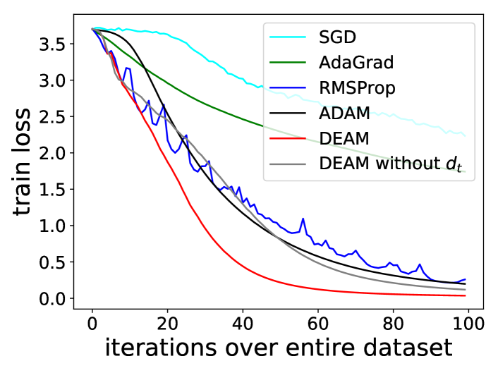
(a) Train loss on ORL

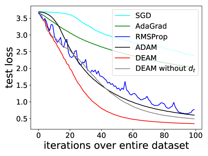
(b) Test loss on ORL

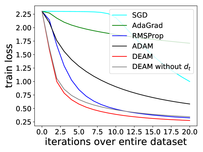
(c) Train loss on MNIST

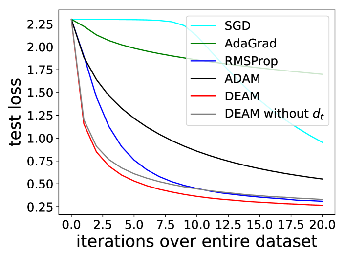
(d) Test loss on MNIST

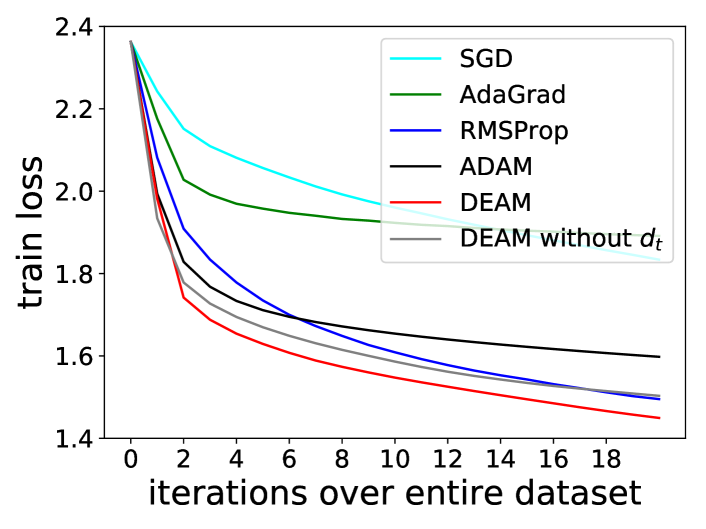
(e) Train loss on CIFAR

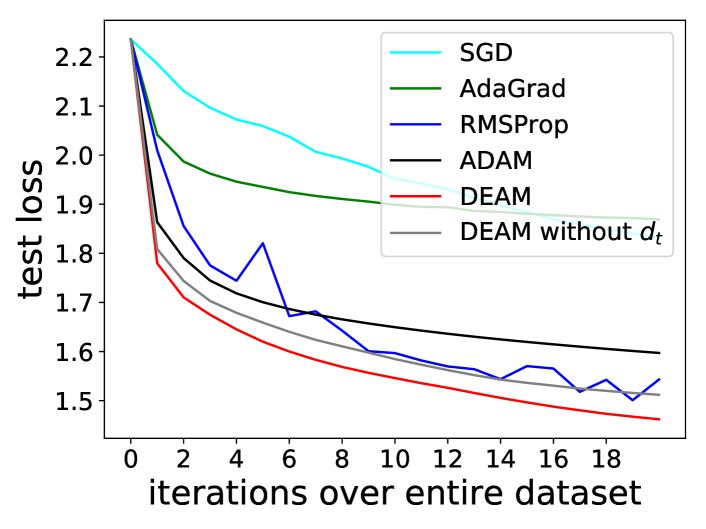
(f) Test loss on CIFAR

Figure 4: Results of CNN structure

Table 1: Running time of DEAM and comparison methods (the unit of values is second)

Comparison Methods	Running time on all models
	Logistic Regression on ORL	DNN on MNIST	CNN on ORL	CNN on MNIST	CNN on CIFAR-10
DEAM	38	302	35064	11679	57761
ADAM	102	664	47418	21775	67584
RMSProp	48	307	36722	11997	84305
AdaGrad	$>200$	667	$>100000$	$>50000$	$>100000$
SGD	$>200$	346	$>100000$	16985	67564

The first inequality is according to Lemma 1. Finally, we will infer the $(11)$ in previous formula. According to the Lemma 2 of Reddi et al. (2018), we have

$$\sum_{t=1}^{T}\frac{\hat{\eta}_{t}}{2\beta_{1,t}}\cdot\frac{\mathbf{m}^{2}_{t,i}}{\sqrt{\mathbf{\hat{v}}_{t,i}}}\leq\frac{1}{2\epsilon_{0}}\sum_{t=1}^{T}\eta_{t}\frac{\mathbf{m}^{2}_{t,i}}{\sqrt{\mathbf{v}_{t,i}}}\leq\frac{\eta}{2\epsilon_{0}}\sum_{t=1}^{T}\frac{1}{\sqrt{t}}\cdot\frac{\mathbf{m}^{2}_{t,i}}{\sqrt{\mathbf{v}_{t,i}}}$$

$$\leq \frac{\eta}{2\epsilon_{0}}\sum_{t=1}^{T}\frac{(\sum_{j=1}^{t}(1-\epsilon_{0})^{t-j})(\sum_{j=1}^{t}(1-\epsilon_{0})^{t-j}\mathbf{g}^{2}_{j,i})}{\sqrt{t((1-\beta_{2})\sum_{j=1}^{t}\beta_{2}^{t-j}\mathbf{g}^{2}_{j,i})}}$$

$$\leq \frac{\eta}{2\epsilon^{2}_{0}\sqrt{1-\beta_{2}}}\sum_{t=1}^{T}\frac{1}{\sqrt{t}}\sum_{j=1}^{t}\frac{(1-\epsilon_{0})^{t-j}\mathbf{g}^{2}_{j,i}}{\sqrt{\beta_{2}^{t-j}\mathbf{g}^{2}_{j,i}}}$$

$$\leq \frac{\eta}{2\epsilon^{2}_{0}\sqrt{1-\beta_{2}}}\sum_{t=1}^{T}|\mathbf{g}_{t,i}|\sum_{j=t}^{T}\frac{\gamma_{1}^{j-t}}{\sqrt{t}}\leq\frac{\eta\sqrt{1+\log T}}{2\epsilon^{2}_{0}(1-\gamma_{1})\sqrt{1-\beta_{2}}}\left\|\mathbf{g}_{1:T,i}\right\|_{2}$$

In the above inequalities, some inferences are based on Cauchy-Schwarz Inequality. Therefore, the final bound of $R(T)$ can be expressed as

$$R(T) \leq\frac{D^{2}}{\epsilon_{0}\eta}\sum_{i=1}^{d}\sqrt{T\mathbf{\hat{v}}_{T,i}}+\frac{(1-\epsilon_{0})^{2}G_{\infty}D_{\infty}d}{K(1-\lambda)^{2}\epsilon_{0}}$$

$$+\frac{\eta\sqrt{1+\log T}}{2\epsilon^{2}_{0}(1-\gamma_{1})\sqrt{1-\beta_{2}}}\sum_{i=1}^{d}\left\|\mathbf{g}_{1:T,i}\right\|_{2}$$

∎

For the bound term, as $T\rightarrow+\infty$, $\frac{R(T)}{T}\rightarrow 0$ and we can infer that $\displaystyle\lim_{T\rightarrow\infty}[f_{t}(\mathbf{w}_{t})-f_{t}(\mathbf{w}^{*})]=0$, which means the proposed algorithm can finally converge.

4 Experiments

We have applied the DEAM algorithm on multiple popular machine learning and deep learning structures, both convex and non-convex situations. To show the advantages of the algorithm, we compare it with various popular optimization algorithms, including ADAM Kingma and Ba (2015), RMSProp Tieleman and Hinton (2012), AdaGrad Duchi et al. (2011) and SGD. For all the experiments, the loss function (objective function) we have selected is the cross-entropy loss function, and the size of the minibatch is 128. Besides, the learning rate is 0.0001.

4.1 Experiment Settings and Results

Logistic Regression: We firstly evaluate our algorithm on the multi-class logistic regression model, since it is widely used and owns a convex objective function. We conduct logistic regression on the ORL dataset Samaria and Harter (1994). ORL dataset consists of face images of 40 people, each person has ten images and each image is in the size of $112\times 92$. The loss of objective functions on both training set and testing set are shown in Figure 3(a), 3(b).

Deep Neural Network: We use deep neural network (DNN) with two fully connected layers of 1,000 hidden units and the Relu Nair and Hinton (2010) activation function. The dataset we use is MNIST LeCun et al. (1998). The MNIST dataset includes 60,000 training samples and 10,000 testing samples, where each sample is a $28\times 28$ image of hand-written numbers from 0 to 9. Result are exhibited in Figure 3(c), 3(d).

Convolutional Neural Network: The CNN models in our experiments are based on the LeNet-5 LeCun et al. (1998), and it is implemented on multiple datasets: ORL, MNIST and CIFAR-10 Krizhevsky (2009). The CIFAR-10 dataset consists of 60,000 $32\times 32$ images in 10 classes, with 6,000 images per class. For different datatsets, the structures of CNN models are modified: for the ORL dataset, the CNN model has two convolutional layers with 16 and 36 feature maps of $5$ kernels and 2 max-pooling layers, and a fully connected layer with 1024 neurons; for the MNIST dataset, the CNN structure follows the LeNet-5 structure in LeCun et al. (1998); for CIFAR-10 dataset, the CNN model consists of three convolutional layers with 64, 128, 256 kernels respectively, and a fully connected layer having 1024 neurons. All experiments apply Relu Nair and Hinton (2010) activation function. The results are shown in Figure 4.

We can observe that DEAM converges faster than other widely used optimization algorithms in all the cases. Within the same number of epoches, DEAM can converge to the lowest loss on both the training set and test set.

4.2 Analysis of the Backtrack Mechanism

To show the effectiveness of the backtrack term $d_{t}$, we also carry out the experiments of DEAM without $d_{t}$ term, and exhibit the results in Figures 3, 4. The results indicate that after applying $d_{t}$ term, the converging speed will become slightly faster. To thoroughly prove the effectiveness of our proposed $d_{t}$ term, we also compare it with other definitions of backtrack terms e.g., $d_{t}=0.5\cos\theta$, and exhibit the results in Figure 5. In Figure 5, $d_{t}=sigmoid\_based$ represents that $d_{t}=-1/(1+e^{-(\theta-\frac{1}{2}\pi)})+\frac{1}{2}$, and $d_{t}=tanh\_based$ means that $d_{t}=-2/(1+e^{-2(x-\frac{1}{2}\pi)})+1$.

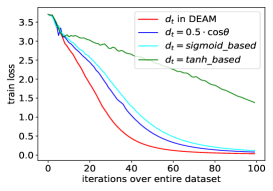
Figure 5: $d_{t}$ terms in other definitions

Due to the limited sapce, here we only exhibit the results on ORL dataset. From the results we can observe that the $d_{t}$ definnition in DEAM achieves the best congerging performance, which means our setting of $d_{t}$ in DEAM is effective.

4.3 Time-consuming Analysis

We have recorded the running time of DEAM and other comparison algorithms in every experiment, and list them in the Table 1. The running time shown in Table 1 contains “$>$”, which means the model still does not converge at the specific time. From the results we can observe that in all of our experiments, DEAM finally converges within the smallest mount of time. From the results in Figures 3,4 and Table 1, we can conclude that DEAM can converge not only in fewer epochs, but using less running time. The device we used is the Dell PowerEdge T630 Tower Server, with 80 cores 64-bit Intel Xeon CPU E5-2698 v4@2.2GHz. The total memory is 256 GB, with an extra (SSD) swap of 250 GB.

5 Conclusion

In this paper, we have introduced a novel optimization algorithm, the DEAM, which implements the momentum with discriminative weights and the backtrack term. We have analyzed the advantages of the proposed algorithm and proved it by theoretical inference. Extensive experiments have shown that the proposed algorithm can converge faster than existing methods on both convex and non-convex situations, and the time consuming is better than existing methods. Not only the proposed algorithm can outperform other popular optimization algorithms, but fewer hyperparameters will be introduced, which makes the DEAM much more applicable.

References

- Bahdanau et al. [2014] Dzmitry Bahdanau, Kyunghyun Cho, and Yoshua Bengio. Neural machine translation by jointly learning to align and translate. In CoRR, 2014.
- Behera et al. [2006] Laxmidhar Behera, Swagat Kumar, and Awhan Patnaik. On adaptive learning rate that guarantees convergence in feedforward networks. IEEE transactions on neural networks, 2006.
- Bianchi and Jakubowicz [2012] Pascal Bianchi and Jérémie Jakubowicz. Convergence of a multi-agent projected stochastic gradient algorithm for non-convex optimization. IEEE Transactions on Automatic Control, 2012.
- Chen et al. [2019] Xiangyi Chen, Sijia Liu, Ruoyu Sun, and Mingyi Hong. On the convergence of a class of adam-type algorithms for non-convex optimization. In ICLR, 2019.
- Dauphin et al. [2015] Yann Dauphin, Harm De Vries, and Yoshua Bengio. Equilibrated adaptive learning rates for non-convex optimization. In NIPS, 2015.
- Dong et al. [2015] Li Dong, Furu Wei, Ming Zhou, and Ke Xu. Question answering over freebase with multi-column convolutional neural networks. In ACL, 2015.
- Dozat [2016] Timothy Dozat. Incorporating nesterov momentum into adam. In ICLR Workshop, 2016.
- Duchi et al. [2011] John Duchi, Elad Hazan, and Yoram Singer. Adaptive subgradient methods for online learning and stochastic optimization. Journal of Machine Learning Research, 2011.
- He et al. [2016] Kaiming He, Xiangyu Zhang, Shaoqing Ren, and Jian Sun. Deep residual learning for image recognition. In CVPR, 2016.
- Keskar and Socher [2017] Nitish Shirish Keskar and Richard Socher. Improving generalization performance by switching from adam to sgd. In arXiv:1712.07628, 2017.
- Kingma and Ba [2015] Diederik P. Kingma and Jimmy Lei Ba. Adam: A method for stochastic optimization. In ICLR, 2015.
- Krizhevsky [2009] Alex Krizhevsky. Learning multiple layers of features from tiny images. In CRC Press, 2009.
- LeCun et al. [1998] Yann LeCun, Leon Bottou, Yoshua Bengio, and Patrick Haffner. Gradient-base learning applied to document recognition. In IEEE, 1998.
- Li et al. [2017] Qunwei Li, Yi Zhou, Yingbin Liang, and Pramod K Varshney. Convergence analysis of proximal gradient with momentum for nonconvex optimization. In ICML, 2017.
- Luo et al. [2019] Liangchen Luo, Yuanhao Xiong, Yan Liu, and Xu Sun. Adaptive gradient methods with dynamic bound of learning rate. In ICLR, 2019.
- Mitliagkas et al. [2016] Ioannis Mitliagkas, Ce Zhang, Stefan Hadjis, and Christopher Ré. Asynchrony begets momentum, with an application to deep learning. In Annual Allerton Conference on Communication, Control, and Computing (Allerton), 2016.
- Nair and Hinton [2010] Vinod Nair and Geoffrey E. Hinton. Rectified linear units improve restricted boltzmann machines. In ICML, 2010.
- Nesterov [1983] Yurii Nesterov. A method for unconstrained convex minimization problem with the rate of convergence o(1/k2). In Doklady ANUSSR, 1983.
- Neumann and Vu [2017] Michael Neumann and Ngoc Thang Vu. Attentive convolutional neural network based speech emotion recognition: A study on the impact of input features, signal length, and acted speech. In CoRR, 2017.
- Qian [1999] Ning Qian. On the momentum term in gradient descent learning algorithms. Neural networks : The Official Journal of the International Neural Network Society, 1999.
- Reddi et al. [2015] Sashank J Reddi, Ahmed Hefny, Suvrit Sra, Barnabas Poczos, and Alexander J Smola. On variance reduction in stochastic gradient descent and its asynchronous variants. In NeurIPS, 2015.
- Reddi et al. [2018] Sashank J. Reddi, Satyen Kale, and Sanjiv Kumar. On the convergence of adam and beyond. In ICLR, 2018.
- Ruder [2017] Sebastian Ruder. An overview of gradient descent optimization algorithms. In arXiv:1609.04747v2, 2017.
- Samaria and Harter [1994] Ferdinando Samaria and Andy Harter. Parameterisation of a stochastic model for human face identification. In IEEE Workshop on Applications of Computer Vision, 1994.
- Sutskever et al. [2013a] Ilya Sutskever, James Martens, George Dahl, and Geoffrey Hinton. On the importance of initialization and momentum in deep learning. In ICML, 2013.
- Sutskever et al. [2013b] Ilya Sutskever, James Martens, George E. Dahl, and Geoffrey E. Hinton. On the importance of initialization and momentum in deep learning. In ICML, 2013.
- Tieleman and Hinton [2012] Tijmen Tieleman and Geoffrey E. Hinton. Leture 6.5 rmsprop,coursera: Neural networks for machine learning. In Tehcnical report, 2012.
- Zeiler [2012] Matthew D. Zeiler. Adadelta: An adaptive learning rate method. In arXiv:1212.5701v1, 2012.
- Zhang et al. [2018] Zijun Zhang, Lin Ma, Zongpeng Li, and Chuan Wu. Normalized direction-preserving adam. In arXiv: 1709.04546v2, 2018.
- Zhang [2019] Jiawei Zhang. Graph neural networks for small graph and giant network representation learning: An overview. Technical report, IFM lab, 2019.
- Zinkevich [2003] Martin Zinkevich. On convex programming and generalized infinitesimal gradient ascent. In ICML, 2003.