Alleviating the sign problem in quantum Monte Carlo simulations of spin-orbit-coupled multiorbital Hubbard models

Aaram J. Kim aaram.kim@kcl.ac.uk Department of Physics, King’s College London, Strand, London WC2R 2LS, UK Philipp Werner Department of Physics, University of Fribourg, Chemin du Musée 3, 1700 Fribourg, Switzerland Roser Valentí Institut für Theoretische Physik, Goethe-Universität Frankfurt, Max-von-Laue-Str. 1, 60438 Frankfurt am Main, Germany

Abstract

We present a strategy to alleviate the sign problem in continuous-time quantum Monte Carlo (CTQMC) simulations of the dynamical-mean-field-theory (DMFT) equations for the spin-orbit-coupled multi-orbital Hubbard model. We first identify the combinations of rotationally invariant Hund coupling terms present in the relativistic basis which lead to a severe sign problem. Exploiting the fact that the average sign in CTQMC depends on the choice of single-particle basis, we propose a bonding-antibonding basis $V_{j3/2\mathrm{BA}}$ which shows an improved average sign compared to the widely used relativistic basis for most parameter sets investigated. We then generalize this procedure by introducing a stochastic optimization algorithm that exploits the space of single-particle bases and show that $V_{j3/2\mathrm{BA}}$ is very close to optimal within the parameter space investigated. Our findings enable more efficient DMFT simulations of materials with strong spin-orbit coupling.

I Introduction

Spin-orbit coupling (SOC) is an essential ingredient in the study of exotic phases in correlated electron systems,Witczak-Krempa et al. (2014) such as unconventional superconductivity in $4d$ transition-metal oxides,Mackenzie and Maeno (2003); Wang and Senthil (2011); Watanabe et al. (2013); Kim et al. (2014a); Yang et al. (2014); Meng et al. (2014); Kim et al. (2015); Borisenko et al. (2015) topological phases of matter in quantum spin-Hall insulators,Kane and Mele (2005); Hasan and Kane (2010); Qi and Zhang (2011) excitonic insulators, Khaliullin (2013); Kuneš (2014); Sato et al. (2015); Kim et al. (2017); Sato et al. (2019) and Kitaev-model-based insulators,Jackeli and Khaliullin (2009); Rau et al. (2016); Savary and Balents (2016); Winter et al. (2017); Hermanns et al. (2018); Takagi et al. (2019) to mention a few. A prototypical minimal model that includes the interplay between spin-orbit coupling and correlations is the relativistic multiorbital Hubbard model. Its nonrelativistic counterpart has been intensively investigated in the past and shows a rich phase diagram.Werner et al. (2008); de’ Medici et al. (2011); Kuneš (2014); Hoshino and Werner (2016) The relativistic multiorbital Hubbard model,Watanabe et al. (2013); Meng et al. (2014); Sato et al. (2015); Shinaoka et al. (2015a); Kim et al. (2017); Sato et al. (2019) however, is much less understood since the choice of algorithms is strongly limited due to the extra computational complications associated with (multiple-)spin-orbit-coupled degrees of freedom.

One of the promising formalisms to investigate the Hubbard model and its generalizations is the dynamical mean-field theory (DMFT) Georges et al. (1996a); Kotliar and Vollhardt (2004) that has provided important insights into multiorbital physics also in combination with ab initio calculations for real materials.Kotliar et al. (2006); Yin et al. (2011); Lechermann et al. (2016) The continuous-time quantum Monte Carlo method (CTQMC),Gull et al. (2011) particularly the hybridization expansion algorithm (CTHYB),Werner et al. (2006); Werner and Millis (2006) is the most widely used impurity solver in multiorbital DMFT calculations. However, CTHYB suffers from the notorious sign problem when the SOC is included in the calculations. The sign problem grows exponentially with inverse temperature Loh et al. (1990); Troyer and Wiese (2005) and typically prevents the study of low-temperature symmetry-broken phases. Alleviating the sign problem in CTHYB would help improve our understanding of phenomena determined by the interplay of spin-orbit coupling and correlations.Mackenzie and Maeno (2003); Kim et al. (2015); Borisenko et al. (2015); Hoshino and Werner (2015); Kim et al. (2018)

For quantum Monte Carlo (QMC) algorithms based on auxiliary fields, there have been various successful advances which unveiled the origin of the sign problem and suggested a solution in specific cases,Chandrasekharan and Wiese (1999); Wang et al. (2015); Iglovikov et al. (2015); Kung et al. (2016); Hann et al. (2017); Yoo et al. (2005); Alet et al. (2016); Huffman and Chandrasekharan (2016); Honecker et al. (2016) including the recently developed idea of Majorana symmetry.Li et al. (2015, 2016); Wei et al. (2016) The rotationally invariant Hund coupling in the SO-coupled multiorbital Hubbard system, however, generates rather complex interaction terms. Furthermore, the nonlocal-in-time expansion scheme of CTHYB makes it difficult to track the origin of the fermionic sign on the world line configuration.

In this paper, we systematically study the nature of the sign problem of the CTHYB for the SO-coupled three-orbital Hubbard model and propose a strategy to alleviate it. We employ a numerical sign-optimization scheme, called spontaneous perturbation stochastic approximation (SPSA),Spall (1992) to determine the optimal basis in terms of average sign. Remarkably, this optimal basis can be well approximated by a simple one, which we denote as $V_{j3/2\mathrm{BA}}$ . The $V_{j3/2\mathrm{BA}}$ basis is obtained from the relativistic basis by a bonding-antibonding transformation.

II Model and Method

Our model Hamiltonian is composed of the three terms $\mathcal{H}=\mathcal{H}_{\text{t}}+\mathcal{H}_{\text{soc}}+\mathcal{H}_{\text{int}}$ , where $\mathcal{H}_{\text{t}}$ , $\mathcal{H}_{\text{soc}}$ , and $\mathcal{H}_{\text{int}}$ are, respectively, the electron hopping, SOC, and Coulomb interaction terms. For the noninteracting electron hopping part we assume a degenerate semicircular density of states $\rho(\omega)=(1/\pi D)\sqrt{1-(\omega/D)^{2}}$ and set the half-bandwidth $D$ as the unit of energy. In the orbital-spin basis $V_{\mathrm{os}}$ , $\mathcal{H}_{\mathrm{soc}}$ has the form

\mathcal{H}_{\text{soc}}=-\lambda\sum_{i}\sum_{\begin{subarray}{c}\alpha\alpha^{\prime}\\ \sigma\sigma^{\prime}\end{subarray}}c^{\dagger}_{i\alpha\sigma}\langle\alpha\sigma|\mathbf{L}_{\text{eff}}\cdot\mathbf{S}|\alpha^{\prime}\sigma^{\prime}\rangle c_{i\alpha^{\prime}\sigma^{\prime}}~{},

(1)

where $\mathbf{L}_{\text{eff}}$ is the $l=1$ orbital angular momentum operator and $\mathbf{S}$ is the spin operator. $c_{i\alpha\sigma}$ ( $c^{\dagger}_{i\alpha\sigma}$ ) is the electron annihilation (creation) operator of orbital $\alpha$ ( $yz,zx,xy$ ) and spin $\sigma$ ( $\uparrow,\downarrow$ ) at lattice site $i$ . We introduce the Slater-Kanamori form of the Coulomb interaction including the spin-flip and pair-hopping terms:

$\displaystyle\mathcal{H}_{\text{int}}$	$\displaystyle=$	$\displaystyle U\sum_{i,\alpha}n_{i\alpha\uparrow}n_{i\alpha\downarrow}+\sum_{\begin{subarray}{c}i,\alpha<\alpha^{\prime}\\ \sigma\sigma^{\prime}\end{subarray}}(U^{\prime}-J_{\rm H}\delta_{\sigma\sigma^{\prime}})n_{i\alpha\sigma}n_{i\alpha^{\prime}\sigma^{\prime}}$	(2)
		$\displaystyle-J_{\rm H}\sum_{i,\alpha<\alpha^{\prime}}(c^{\dagger}_{i\alpha\uparrow}c^{\dagger}_{i\alpha^{\prime}\downarrow}c_{i\alpha^{\prime}\uparrow}c_{i\alpha\downarrow}+\text{H.c.})$
		$\displaystyle+J_{\rm H}\sum_{i,\alpha<\alpha^{\prime}}(c^{\dagger}_{i\alpha\uparrow}c^{\dagger}_{i\alpha\downarrow}c_{i\alpha^{\prime}\downarrow}c_{i\alpha^{\prime}\uparrow}+\text{H.c.})~{}.$

Here, $U$ ( $U^{\prime}$ ) is the intraorbital (interorbital) Coulomb repulsion, and $J_{\text{H}}$ is the strength of the Hund coupling. To make $\mathcal{H}_{\mathrm{int}}$ rotationally invariant, we choose $U^{\prime}=U-2J_{\mathrm{H}}$ . This model Hamiltonian covers a wide range of $4d$ and $5d$ materials listed in Appendix A by tuning the electron density, $\lambda$ , $U$ , and $J_{\mathrm{H}}$ .

We solve the model Hamiltonian within the framework of DMFT.Georges et al. (1996b) The lattice model is mapped onto a quantum impurity model by means of a self-consistency relation. The effective action of the quantum impurity model is written in terms of the local action $\mathcal{S}_{\mathrm{loc}}$ and the hybridization function $\Delta$ ,

	$\displaystyle\mathcal{S}_{\text{imp}}$	$\displaystyle=$	$\displaystyle\mathcal{S}_{\text{loc}}$
		$\displaystyle+$	$\displaystyle\sum_{\begin{subarray}{c}\alpha\alpha^{\prime}\\ \sigma\sigma^{\prime}\end{subarray}}\int_{0}^{\beta}d\tau d\tau^{\prime}~{}c^{\dagger}_{\alpha\sigma}(\tau)\Delta_{\alpha\sigma,\alpha^{\prime}\sigma^{\prime}}(\tau-\tau^{\prime})c_{\alpha^{\prime}\sigma^{\prime}}(\tau^{\prime})~{}.$

Here, $c_{\alpha\sigma}$ and $c^{\dagger}_{\alpha\sigma}$ are the fermionic annihilation and creation operators for orbital $\alpha$ and spin $\sigma$ for the impurity site. CTHYB solves this impurity problem by performing an expansion of the partition function in powers of the hybridization function,

$\displaystyle\mathcal{Z}_{\text{imp}}$	$\displaystyle=$	$\displaystyle\mathcal{Z}_{\mathrm{bath}}\sum^{\infty}_{k=0}\frac{1}{(k!)^{2}}\sum_{\begin{subarray}{c}\alpha_{1}\alpha^{\prime}_{1}\\ \sigma_{1}\sigma^{\prime}_{1}\end{subarray}}\cdots\sum_{\begin{subarray}{c}\alpha_{k}\alpha^{\prime}_{k}\\ \sigma_{k}\sigma^{\prime}_{k}\end{subarray}}$
	$\displaystyle\times$	$\displaystyle\int_{0}^{\beta}d\tau_{1}\int_{0}^{\beta}d\tau^{\prime}_{1}\cdots\int_{0}^{\beta}d\tau_{k}\int_{0}^{\beta}d\tau^{\prime}_{k}~{}\det\left[\underline{\Delta}^{(k)}\right]$
	$\displaystyle\times$	$\displaystyle\left\langle\mathcal{T}_{\tau}c_{\alpha^{\prime}_{1}\sigma^{\prime}_{1}}(\tau^{\prime}_{1})c^{\dagger}_{\alpha_{1}\sigma_{1}}(\tau_{1})\cdots c_{\alpha^{\prime}_{k}\sigma^{\prime}_{k}}(\tau^{\prime}_{k})c^{\dagger}_{\alpha_{k}\sigma_{k}}(\tau_{k})\right\rangle_{\mathcal{S}_{\mathrm{loc}}}.$

Here, $\underline{\Delta}^{(k)}$ represents the $k\times k$ matrix whose elements are

\underline{\Delta}^{(k)}_{ij}=\Delta_{\alpha_{i}\sigma_{i},\alpha^{\prime}_{j}\sigma^{\prime}_{j}}(\tau_{i}-\tau^{\prime}_{j})~{}.

(5)

The hybridization function contains the relevant information about the continuous bath degrees of freedom. Since $\Delta$ is directly updated in the DMFT self-consistency loop, CTHYB does not rely on a discretization or truncation of the bath, in contrast to other impurity solvers like the exact diagonalization or the numerical renormalization group.Georges et al. (1996a); Gull et al. (2011) In that sense, CTHYB is numerically exact in treating the bath degrees of freedom.

The resulting partition function, Eq. (LABEL:eqn:Zimp), can be expressed as a sum of configuration weights,

\mathcal{Z}_{\text{imp}}=\sum_{\mathbf{x}}\omega(\mathbf{x})

(6)

where

\omega(\mathbf{x})=\mathcal{Z}_{\text{bath}}\frac{(d\tau)^{2k}}{(k!)^{2}}\left\langle\mathcal{T}_{\tau}c_{\alpha^{\prime}_{1}\sigma^{\prime}_{1}}(\tau^{\prime}_{1})c^{\dagger}_{\alpha_{1}\sigma_{1}}(\tau_{1})\cdots c_{\alpha^{\prime}_{k}\sigma^{\prime}_{k}}(\tau^{\prime}_{k})c^{\dagger}_{\alpha_{k}\sigma_{k}}(\tau_{k})\right\rangle_{\mathcal{S}_{\mathrm{loc}}}\det\left[\underline{\Delta}^{(k)}\right]~{}.

(7)

Here, $\mathbf{x}$ represents the configuration composed of $\left\{k;(\alpha_{1},\sigma_{1},\tau_{1}),(\alpha^{\prime}_{1},\sigma^{\prime}_{1},\tau^{\prime}_{1}),\dots(\alpha_{k},\sigma_{k},\tau_{k}),(\alpha^{\prime}_{k},\sigma^{\prime}_{k},\tau^{\prime}_{k})\right\}$ . One can measure a general time-local observable $\mathcal{O}$ using MC sampling as

\langle\mathcal{O}\rangle_{\text{MC}}=\frac{\sum_{\mathbf{x}}\mathcal{O}(\mathbf{x})\omega(\mathbf{x})}{\sum_{\mathbf{x}}\omega(\mathbf{x})}~{}.

(8)

A potential sign problem appears when the weight $\omega(\mathbf{x})$ becomes negative for certain configurations. In this case the observable can be sampled through the modified expression

\langle\mathcal{O}\rangle_{\text{MC}}=\frac{\sum_{\mathbf{x}}\text{sign}[\omega(\mathbf{x})]~{}\mathcal{O}(\mathbf{x})~{}|\omega(\mathbf{x})|}{\sum_{\mathbf{x}}\text{sign}[\omega(\mathbf{x})]~{}|\omega(\mathbf{x})|}~{}.

(9)

A severe sign problem occurs if the small average sign

\langle\mathrm{sign}\rangle=\frac{\sum_{\mathbf{x}}\mathrm{sign}[\omega(\mathbf{x})]|\omega(\mathbf{x})|}{\sum_{\mathbf{x}}|\omega(\mathbf{x})|}

(10)

amplifies the error propagation in the estimation of the observables. Especially, for low temperatures, the relative error of the average sign becomes exponentially large as a function of the inverse temperature $\beta$ . Thus, reliable estimates of observables cannot be obtained in polynomial time. An analogous phase problem appears if the configuration weights are complex. However, since the average phase is always real, we will for simplicity use the terms sign problem and average sign in the following.

An important aspect to keep in mind is that the sign problem depends on the single-particle basis. For example, it has been reported that if the electron operators $\tilde{c}_{j,m}$ are expressed in the relativistic $j_{\text{eff}}$ basis $V_{j\mathrm{eff}}$ ,

	$\displaystyle\left(\begin{array}[]{c}\tilde{c}_{\frac{1}{2},+\frac{1}{2}}\\ \tilde{c}_{\frac{3}{2},+\frac{1}{2}}\\ \tilde{c}_{\frac{3}{2},-\frac{3}{2}}\end{array}\right)$	$\displaystyle=$	$\displaystyle\frac{1}{\sqrt{6}}\left(\begin{array}[]{ccc}-\sqrt{2}&+i\sqrt{2}&-\sqrt{2}\\ -1&i&2\\ -\sqrt{3}&i\sqrt{3}&0\\ \end{array}\right)\left(\begin{array}[]{c}c_{yz,\downarrow}\\ c_{zx,\downarrow}\\ c_{xy,\uparrow}\\ \end{array}\right)~{},$		(20)
	$\displaystyle\left(\begin{array}[]{c}\tilde{c}_{\frac{1}{2},-\frac{1}{2}}\\ \tilde{c}_{\frac{3}{2},-\frac{1}{2}}\\ \tilde{c}_{\frac{3}{2},+\frac{3}{2}}\end{array}\right)$	$\displaystyle=$	$\displaystyle\frac{1}{\sqrt{6}}\left(\begin{array}[]{ccc}-\sqrt{2}&-i\sqrt{2}&+\sqrt{2}\\ +1&i&2\\ +\sqrt{3}&i\sqrt{3}&0\\ \end{array}\right)\left(\begin{array}[]{c}c_{yz,\uparrow}\\ c_{zx,\uparrow}\\ c_{xy,\downarrow}\\ \end{array}\right),\hskip 22.76219pt$		(30)

the average sign is improved Sato et al. (2015) due to the diagonalized hybridization function matrix.Meng et al. (2014) (An average sign of 1 means no sign problem, while an average sign approaching 0 means a severe sign problem.)

To further optimize the basis beyond $V_{j\mathrm{eff}}$ , we introduce the numerical optimization scheme SPSA. In this scheme the average sign becomes the objective function on the parameter space where each point corresponds to a single-particle basis used in CTHYB. The SPSA approximates the gradient for a given parameter point. At each iteration, the objective function is measured at both the positively and negatively perturbed parameter points along a stochastically chosen direction. The gradient is evaluated from this two-point measurement, and the parameter point is updated. Compared to the finite-difference stochastic approximation which involves a number of measurements proportional to the dimension of the parameter space, the SPSA potentially converges faster in time if the parameter space is high-dimensional and the measurement of the objective function is computationally expensive.

Refer to caption — Figure 1: Average sign for four different bases as a function of (a) the electron density $n$ and (b) and (c) the strength of SOC $\lambda$ for $T=0.03$ , $U=2.0$ , and $J_{\mathrm{H}}/U=0.15$ . $V_{\mathrm{opt}}$ , $V_{j3/2\mathrm{BA}}$ , $V_{j\mathrm{eff}}$ , and $V_{\mathrm{os}}$ represent, respectively, the optimal basis found by the SPSA, the $j=3/2$ bonding-antibonding basis, the $j_{\mathrm{eff}}$ basis, and the orbital-spin basis. The average sign is calculated using the self-consistent paramagnetic solution for a given parameter set. The open squares and circles at $n=3$ correspond to the average signs of the Mott insulator solution.

III Results

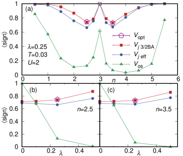
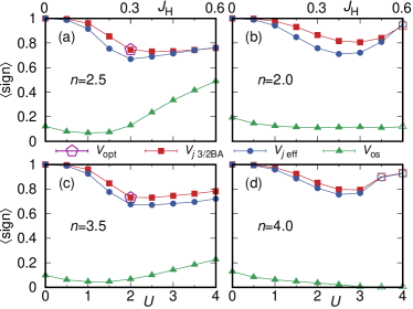
In Fig. 1 we plot the average sign for the four different bases considered in this work as a function of electron density [Fig. 1(a)] and spin-orbit coupling strength [Fig. 1(b) and (c)]. The orbital-spin basis $V_{\mathrm{os}}$ has a severe sign problem since a drastic drop in the average sign of $V_{\mathrm{os}}$ appears as a function of the SOC strength both below and above half-filling. Figure 2 shows the evolution of the average sign as a function of $U$ ( $J_{\mathrm{H}}$ ) at various electron fillings. The suppressed average sign of $V_{\mathrm{os}}$ in the noninteracting limit implies that the source of the sign problem in this basis is the off-diagonal hybridization function generated by the SOC. The basis $V_{j\mathrm{eff}}$ , defined in Eq. (30), diagonalizes the hybridization-function matrix of the Hamiltonian and thus recovers the sign-free behavior in the noninteracting limit, as demonstrated in Fig. 2. In the presence of a nonzero Hund coupling $J_{\mathrm{H}}$ , however, $V_{j\mathrm{eff}}$ shows a sign problem as well, especially at intermediate interaction strengths and away from half-filling.

In order to further improve the average sign we introduce the basis $V_{j3/2\mathrm{BA}}$ in which $\tilde{c}_{\frac{3}{2},+\frac{3}{2}}$ and $\tilde{c}_{\frac{3}{2},-\frac{3}{2}}$ are mixed in the bonding-antibonding manner:

\left(\begin{array}[]{c}\tilde{a}_{\frac{3}{2},+}\\ \tilde{a}_{\frac{3}{2},-}\end{array}\right)=\frac{1}{\sqrt{2}}\left(\begin{array}[]{cccccc}1&1\\ 1&-1\\ \end{array}\right)\left(\begin{array}[]{c}\tilde{c}_{\frac{3}{2},+\frac{3}{2}}\\ \tilde{c}_{\frac{3}{2},-\frac{3}{2}}\end{array}\right)~{}.\\

(31)

A similar transformation was previously explored for an isolated trimer.Shinaoka et al. (2015b) It turns out that $V_{j3/2\mathrm{BA}}$ is superior to $V_{j\mathrm{eff}}$ for most parameter sets investigated. In the noninteracting limit, $V_{j3/2\mathrm{BA}}$ (like $V_{j\mathrm{eff}}$ ) yields an average sign of unity (see Fig. 2). As $U$ is switched on, $V_{j3/2\mathrm{BA}}$ results in a larger average sign than $V_{j\mathrm{eff}}$ . In Fig. 2, the improvement of the average sign in $V_{j3/2\mathrm{BA}}$ is prominent in the itinerant regime with intermediate Coulomb interaction strength. This improvement persists over the whole range of electron densities for $U=2$ as shown in Fig 1(a) . In the Mott insulating regime (marked by open squares and circles in Figs. 1 and 2), on the other hand, the difference between the average signs of $V_{j3/2\mathrm{BA}}$ and $V_{j\mathrm{eff}}$ is smaller. Since the CTHYB is based on the expansion around the localized limit, those observations imply that $V_{j3/2\mathrm{BA}}$ effectively prevents sign-problematic high-order processes.

Note that neither $V_{j3/2\mathrm{BA}}$ nor $V_{j\mathrm{eff}}$ is an optimal basis for the non-SO-coupled model. As we show in Figs. 1(b) and (c), at the non-SO-coupled point ( $\lambda=0$ ), $V_{j3/2\mathrm{BA}}$ and $V_{j\mathrm{eff}}$ exhibit a sign problem, in contrast to $V_{\mathrm{os}}$ . This demonstrates that Eq. (2) includes dangerous interacting terms in the $V_{j3/2\mathrm{BA}}$ and $V_{j\mathrm{eff}}$ basis. One of these terms is the correlated-hopping (CH) term, which has the form

	$\displaystyle\frac{\sqrt{2}J_{\text{H}}}{3}\sum_{s=\pm}\left[s(2\tilde{n}_{\frac{3}{2},s\frac{3}{2}}-\tilde{n}_{\frac{3}{2},\bar{s}\frac{3}{2}}-\tilde{n}_{\frac{3}{2},\bar{s}\frac{1}{2}})\tilde{c}^{\dagger}_{\frac{1}{2},s\frac{1}{2}}\tilde{c}_{\frac{3}{2},s\frac{1}{2}}+\text{H.c.}\right]$
			(32)

in $V_{j\mathrm{eff}}$ and

	$\displaystyle\frac{\sqrt{2}J_{\text{H}}}{6}\sum_{s=\pm}\left[s(\tilde{n}_{\frac{3}{2},+}+\tilde{n}_{\frac{3}{2},-}-2\tilde{n}_{\frac{3}{2},\bar{s}\frac{1}{2}})\tilde{c}^{\dagger}_{\frac{1}{2},s\frac{1}{2}}\tilde{c}_{\frac{3}{2},s\frac{1}{2}}+\text{H.c.}\right]$
	$\displaystyle+\frac{J_{\mathrm{H}}}{2}\left[(\tilde{n}_{\frac{1}{2},+\frac{1}{2}}-\tilde{n}_{\frac{1}{2},-\frac{1}{2}})\tilde{a}^{\dagger}_{\frac{3}{2},+}a_{\frac{3}{2},-}+\text{H.c.}\right]$		(33)

in $V_{j3/2\mathrm{BA}}$ . This CH term is the major source of the sign problem in the SO-coupled Hamiltonian. Table 1 analyzes the effect of different terms in the local Hamiltonian on the average sign for both $V_{j3/2\mathrm{BA}}$ and $V_{j\mathrm{eff}}$ . There is a substantial drop in the average sign when the CH terms are introduced.

Terms	$\langle\mathrm{sign}\rangle_{V_{j\mathrm{eff}}}$	$\langle\mathrm{sign}\rangle_{V_{j3/2\mathrm{BA}}}$
Density-density (DD)	1.00000	1.00000
DD + spin flip (SF)	1.00000	1.00000
DD + four scattering (FS)	0.99447(9)	0.9516(3)
DD + SF + pair hopping (PH)	0.9760(2)	0.9739(2)
DD + PH	0.9730(7)	0.9705(2)
DD + SF + PH + FS	0.9308(3)	0.9035(6)
DD + correlated hopping (CH)	0.8212(9)	0.8730(5)
DD + CH + FS	0.8061(6)	0.7718(5)
DD + PH + CH	0.7728(6)	0.8623(6)
DD + SF + PH + CH	0.7638(7)	0.8814(5)
DD + SF + PH + CH + FS	0.6751(8)	0.7406(4)

Table 1: Average sign for the masked local Hamiltonians represented in

V_{j\mathrm{eff}}

and

V_{j3/2\mathrm{BA}}

. The results are for

n=3.5

T=0.03

\lambda=0.25

U=2.0

, and

J_{\mathrm{H}}/U

=0.15, and the self-consistent hybridization for the full local Hamiltonian.

In $V_{j3/2\mathrm{BA}}$ and $V_{j\mathrm{eff}}$ , there emerge other new terms involving four different flavors, which are not of the spin-flip type or pair-hopping type appearing in the Slater-Kanamori Hamiltonian in $V_{\mathrm{os}}$ . Those terms are denoted as four-scattering terms in Table 1 . The average sign in both $V_{j3/2\mathrm{BA}}$ and $V_{j\mathrm{eff}}$ becomes even lower when the CH term is combined with the pair-hopping and the four-scattering terms. The full interacting Hamiltonian in $V_{j\text{eff}}$ is explicitly written in Appendix B. Furthermore, we analyze the nature of the self-consistent solutions for the Hamiltonians without the CH or FS terms and we discuss the potential use of such masked Hamiltonians in Appendix C.

In what follows we will determine by the SPSA method the optimal basis in terms of the average sign for the parameters with the most severe sign problem and show that this optimal basis is nearly identical to the $V_{j3/2\mathrm{BA}}$ basis. For that, we search the basis space generated by the $SO(4)$ rotation group for $j=3/2$ , whose $4\times 4$ matrix representation is denoted by $\mathbbm{M}$ and transforms the electron operators in $V_{j\mathrm{eff}}$ as follows:

	$\displaystyle\tilde{a}_{\frac{3}{2}}=\mathbbm{M}\cdot\tilde{c}_{\frac{3}{2}}~{},$		(34)
	$\displaystyle\tilde{a}^{\intercal}_{\frac{3}{2}}=\left(\tilde{a}_{\frac{3}{2},1},\tilde{a}_{\frac{3}{2},2},\tilde{a}_{\frac{3}{2},3},\tilde{a}_{\frac{3}{2},4}\right)~{},$		(35)
	$\displaystyle\tilde{c}^{\intercal}_{\frac{3}{2}}=\left(\tilde{c}_{\frac{3}{2},+\frac{1}{2}},\tilde{c}_{\frac{3}{2},-\frac{1}{2}},\tilde{c}_{\frac{3}{2},+\frac{3}{2}},\tilde{c}_{\frac{3}{2},-\frac{3}{2}}\right)~{}.$		(36)

Since the off-diagonal hybridization function is a clear source of the severe sign problem as shown in the cases of $V_{\mathrm{os}}$ (Figs. 1 and 2), we exclude the mixing between the $j=1/2$ and $3/2$ subspaces to preserve the diagonal structure of the hybridization. Without mixing between the $j=1/2$ and $3/2$ subspaces, one can fix the basis for the $j=1/2$ subspace using the rotational symmetry generated by the total angular momentum operator, $\mathbf{J}_{\mathrm{eff}}=\mathbf{L}_{\mathrm{eff}}+\mathbf{S}$ without loss of generality.

To parametrize the basis space, we introduce the isoclinic decomposition of $\mathbbm{M}$ as $\mathbbm{M}=\mathbbm{M}_{L}\mathbbm{M}_{R}$ , where

\displaystyle\mathbbm{M}_{L}{=}\left(\begin{array}[]{cccc}a&-b&-c&-d\\ b&a&-d&c\\ c&d&a&-b\\ d&-c&b&a\end{array}\right),\hskip 5.69054pt\mathbbm{M}_{R}{=}\left(\begin{array}[]{cccc}p&-q&-r&-s\\ q&p&s&-r\\ r&-s&p&q\\ s&r&-q&p\end{array}\right).

(45)

Here, $a^{2}+b^{2}+c^{2}+d^{2}=1$ and $p^{2}+q^{2}+r^{2}+s^{2}=1$ . Under these constraints among $\{a,b,c,d\}$ and $\{p,q,r,s\}$ the dimension of the parameter space becomes $6$ .

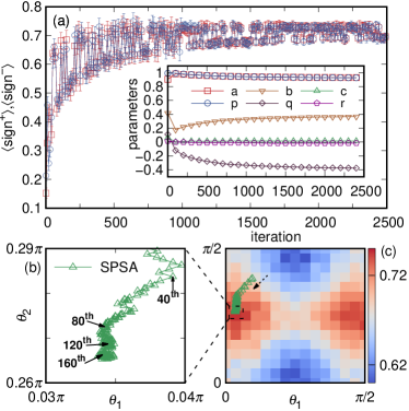
Figure 3 shows how the SPSA works while searching for the optimal basis in this parameter space. The evolution of the average sign as a function of number of iterations at both positively ( $\langle\mathrm{sign}^{+}\rangle$ ) and negatively ( $\langle\mathrm{sign}^{-}\rangle$ ) perturbed points in the parameter space is shown in Fig. 3 (a). The average sign value converges to $\sim 0.74$ for $n=3.5$ , $T=0.03$ , $\lambda=0.25$ , $U=2.0$ , and $J_{\mathrm{H}}/U=0.15$ . Within numerical accuracy, it is very close to the value of $V_{j3/2\mathrm{BA}}$ defined in Eq. (31) . This shows that the $V_{j3/2\mathrm{BA}}$ basis is at least near the local optimum in parameter space. The inset of Fig. 3(a) illustrates the convergence of the parameters in Eqs. (45).

Figure 3(b) and (c) show the SPSA sequence in a small parameter subspace. We introduce two parameters, $\theta_{1}$ and $\theta_{2}$ , representing the restricted basis transformation

\mathbbm{M}=\left(\begin{array}[]{cccc}\cos\theta_{1}&\sin\theta_{1}&0&0\\ -\sin\theta_{1}&\cos\theta_{1}&0&0\\ 0&0&\cos\theta_{2}&\sin\theta_{2}\\ 0&0&-\sin\theta_{2}&\cos\theta_{2}\\ \end{array}\right)~{}.

(46)

Figure 3(c) shows that the landscape of the average sign is smooth, so that the SPSA search based on the gradient approximation can successfully find the local optimum in that subspace. Furthermore, $V_{j3/2\mathrm{BA}}$ , corresponding to $\theta_{1}=0$ and $\theta_{2}=\pi/4$ , is shown to be very close to the optimum found by the SPSA. Figure 3(b) plots the trajectory determined by the SPSA.

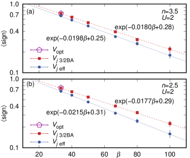
We finally investigate the temperature scaling of the average sign for the different bases. Figure 4 shows the exponential scaling $\langle\mathrm{sign}\rangle\sim\exp\left(-\beta\delta F+F_{0}\right)$ as a function of the inverse temperature $\beta$ . Here, $\delta F$ can be regarded as the free-energy difference from the auxiliary bosonic system without a sign problem, which determines the temperature scaling. For both fillings, $n=3.5$ and $2.5$ , the $V_{j3/2\mathrm{BA}}$ basis shows an improved temperature scaling exponent $\delta F$ and a comparable offset $F_{0}$ .

IV Conclusion

We have investigated the nature of the sign problem in the CTHYB for the SO-coupled multiorbital Hubbard model. We found that the correlated hopping term that appears in the $j_{\mathrm{eff}}$ basis is the major source of the sign problem, and we introduced a basis–the $j=3/2$ bonding-antibonding basis–which alleviates the effects of those terms. By applying the stochastic optimization scheme, we found that the $j=3/2$ bonding-antibonding basis is near a local optimum in the parameter space considered. These results (i) provide useful guidelines for the choice of the single-particle basis in CTHYB simulations of SO-coupled systems, (ii) introduce an algorithm to numerically determine the optimal basis, and (iii) suggest using the intrinsic fermionic sign bound in a systematic search of the full $SO(4)$ basis space as a strategy for the further improvement of CTHYB for this class of systems.

In addition, our findings have relevance for descriptions beyond DMFT that include nonlocal correlations. For example, since the average sign is alleviated at the level of the partition function in $V_{j3/2\text{BA}}$ , we expect our results to be helpful for a reliable estimation of two-particle correlation functions, which are the essential building blocks of diagrammatic extensions of DMFT.Rohringer et al. (2018) For cluster extensions of DMFT, on the other hand, our numerical basis optimization scheme can be applied to an extended basis space including site (cluster) degrees of freedom. A promising strategy might be to combine the $V_{j3/2\text{BA}}$ basis with a bonding-antibonding transformation that breaks loops on the cluster.Shinaoka et al. (2015b)

Note added. During the final stages of this work, a series of conceptually related studies appeared on arXiv.Hangleiter et al. ; Torlai et al. ; Levy and Clark

Acknowledgements.

A.J.K. was supported by EPSRC through Grant No. EP/P003052/1. P.W. acknowledges support from the Swiss National Science Foundation via NCCR Marvel. R.V. acknowledges support by the Deutsche Forschungsgemeinschaft (DFG) through Grant No. VA117/15-1. The computations were performed at the Centre for Scientific Computing (CSC) in Frankfurt.

References

Witczak-Krempa et al. (2014) W. Witczak-Krempa, G. Chen, Y. B. Kim, and L. Balents, Annu. Rev. Condens. Matter Phys 5, 57 (2014).
Mackenzie and Maeno (2003) A. P. Mackenzie and Y. Maeno, Rev. Mod. Phys. 75, 657 (2003).
Wang and Senthil (2011) F. Wang and T. Senthil, Phys. Rev. Lett. 106, 136402 (2011).
Watanabe et al. (2013) H. Watanabe, T. Shirakawa, and S. Yunoki, Phys. Rev. Lett. 110, 027002 (2013).
Kim et al. (2014a) Y. K. Kim, O. Krupin, J. D. Denlinger, A. Bostwick, E. Rotenberg, Q. Zhao, J. F. Mitchell, J. W. Allen, and B. J. Kim, Science 345, 187 (2014a).
Yang et al. (2014) Y. Yang, W.-S. Wang, J.-G. Liu, H. Chen, J.-H. Dai, and Q.-H. Wang, Phys. Rev. B 89, 094518 (2014).
Meng et al. (2014) Z. Y. Meng, Y. B. Kim, and H.-Y. Kee, Phys. Rev. Lett. 113, 177003 (2014).
Kim et al. (2015) Y. K. Kim, N. H. Sung, J. D. Denlinger, and B. J. Kim, Nat. Phys. 12, 37 (2015).
Borisenko et al. (2015) S. V. Borisenko, D. V. Evtushinsky, Z. H. Liu, I. Morozov, R. Kappenberger, S. Wurmehl, B. Büchner, A. N. Yaresko, T. K. Kim, M. Hoesch, T. Wolf, and N. D. Zhigadlo, Nat. Phys. 12, 311 (2015).
Kane and Mele (2005) C. L. Kane and E. J. Mele, Phys. Rev. Lett. 95, 226801 (2005).
Hasan and Kane (2010) M. Z. Hasan and C. L. Kane, Rev. Mod. Phys. 82, 3045 (2010).
Qi and Zhang (2011) X.-L. Qi and S.-C. Zhang, Rev. Mod. Phys. 83, 1057 (2011).
Khaliullin (2013) G. Khaliullin, Phys. Rev. Lett. 111, 197201 (2013).
Kuneš (2014) J. Kuneš, Phys. Rev. B 90, 235140 (2014).
Sato et al. (2015) T. Sato, T. Shirakawa, and S. Yunoki, Phys. Rev. B 91, 125122 (2015).
Kim et al. (2017) A. J. Kim, H. O. Jeschke, P. Werner, and R. Valentí, Phys. Rev. Lett. 118, 086401 (2017).
Sato et al. (2019) T. Sato, T. Shirakawa, and S. Yunoki, Phys. Rev. B 99, 075117 (2019).
Jackeli and Khaliullin (2009) G. Jackeli and G. Khaliullin, Phys. Rev. Lett. 102, 017205 (2009).
Rau et al. (2016) J. G. Rau, E. K.-H. Lee, and H.-Y. Kee, Annu. Rev. Condens. Matter Phys. 7, 195 (2016).
Savary and Balents (2016) L. Savary and L. Balents, Rep. Prog. Phys. 80 (2016).
Winter et al. (2017) S. M. Winter, A. A. Tsirlin, M. Daghofer, J. Van Den Brink, Y. Singh, P. Gegenwart, and R. Valentí, Journal of Physics Condensed Matter 29 (2017).
Hermanns et al. (2018) M. Hermanns, I. Kimchi, and J. Knolle, Annu. Rev. Condens. Matter Phys. 9, 17 (2018).
Takagi et al. (2019) H. Takagi, T. Takayama, G. Jackeli, G. Khaliullin, and S. E. Nagler, Nat. Rev. Phys. 1, 264 (2019).
Werner et al. (2008) P. Werner, E. Gull, M. Troyer, and A. J. Millis, Phys. Rev. Lett. 101, 166405 (2008).
de’ Medici et al. (2011) L. de’ Medici, J. Mravlje, and A. Georges, Phys. Rev. Lett. 107, 256401 (2011).
Hoshino and Werner (2016) S. Hoshino and P. Werner, Phys. Rev. B 93, 155161 (2016).
Shinaoka et al. (2015a) H. Shinaoka, S. Hoshino, M. Troyer, and P. Werner, Phys. Rev. Lett. 115, 156401 (2015a).
Georges et al. (1996a) A. Georges, G. Kotliar, W. Krauth, and M. J. Rozenberg, Rev. Mod. Phys. 68, 13 (1996a).
Kotliar and Vollhardt (2004) G. Kotliar and D. Vollhardt, Phys. Today 57, 53 (2004).
Kotliar et al. (2006) G. Kotliar, S. Y. Savrasov, K. Haule, V. S. Oudovenko, O. Parcollet, and C. A. Marianetti, Rev. Mod. Phys. 78, 865 (2006).
Yin et al. (2011) Z. Yin, K. Haule, and G. Kotliar, Nat. Mater. 10, 932 (2011).
Lechermann et al. (2016) F. Lechermann, H. O. Jeschke, A. J. Kim, S. Backes, and R. Valentí, Phys. Rev. B 93, 121103(R) (2016).
Gull et al. (2011) E. Gull, A. J. Millis, A. I. Lichtenstein, A. N. Rubtsov, M. Troyer, and P. Werner, Rev. Mod. Phys. 83, 349 (2011).
Werner et al. (2006) P. Werner, A. Comanac, L. de’ Medici, M. Troyer, and A. J. Millis, Phys. Rev. Lett. 97, 076405 (2006).
Werner and Millis (2006) P. Werner and A. J. Millis, Phys. Rev. B 74, 155107 (2006).
Loh et al. (1990) E. Y. Loh, J. E. Gubernatis, R. T. Scalettar, S. R. White, D. J. Scalapino, and R. L. Sugar, Phys. Rev. B 41, 9301 (1990).
Troyer and Wiese (2005) M. Troyer and U.-J. Wiese, Phys. Rev. Lett. 94, 170201 (2005).
Hoshino and Werner (2015) S. Hoshino and P. Werner, Phys. Rev. Lett. 115, 247001 (2015).
Kim et al. (2018) M. Kim, J. Mravlje, M. Ferrero, O. Parcollet, and A. Georges, Phys. Rev. Lett. 120, 126401 (2018).
Chandrasekharan and Wiese (1999) S. Chandrasekharan and U.-J. Wiese, Phys. Rev. Lett. 83, 3116 (1999).
Wang et al. (2015) L. Wang, Y.-H. Liu, M. Iazzi, M. Troyer, and G. Harcos, Phys. Rev. Lett. 115, 250601 (2015).
Iglovikov et al. (2015) V. I. Iglovikov, E. Khatami, and R. T. Scalettar, Phys. Rev. B 92, 045110 (2015).
Kung et al. (2016) Y. F. Kung, C. C. Chen, Y. Wang, E. W. Huang, E. A. Nowadnick, B. Moritz, R. T. Scalettar, S. Johnston, and T. P. Devereaux, Phys. Rev. B 93, 155166 (2016).
Hann et al. (2017) C. T. Hann, E. Huffman, and S. Chandrasekharan, Ann. Phys. (N. Y.) 376, 63 (2017).
Yoo et al. (2005) J. Yoo, S. Chandrasekharan, R. K. Kaul, D. Ullmo, and H. U. Baranger, J. Phys. A 38, 10307 (2005).
Alet et al. (2016) F. Alet, K. Damle, and S. Pujari, Phys. Rev. Lett. 117, 197203 (2016).
Huffman and Chandrasekharan (2016) E. Huffman and S. Chandrasekharan, Phys. Rev. E 94, 043311 (2016).
Honecker et al. (2016) A. Honecker, S. Wessel, R. Kerkdyk, T. Pruschke, F. Mila, and B. Normand, Phys. Rev. B 93, 054408 (2016).
Li et al. (2015) Z.-X. Li, Y.-F. Jiang, and H. Yao, Phys. Rev. B 91, 241117(R) (2015).
Li et al. (2016) Z.-X. Li, Y.-F. Jiang, and H. Yao, Phys. Rev. Lett. 117, 267002 (2016).
Wei et al. (2016) Z. C. Wei, C. Wu, Y. Li, S. Zhang, and T. Xiang, Phys. Rev. Lett. 116, 250601 (2016).
Spall (1992) J. C. Spall, IEEE Trans. Autom. Control 37, 332 (1992).
Georges et al. (1996b) A. Georges, G. Kotliar, W. Krauth, and M. J. Rozenberg, Rev. Mod. Phys. 68, 13 (1996b).
Shinaoka et al. (2015b) H. Shinaoka, Y. Nomura, S. Biermann, M. Troyer, and P. Werner, Phys. Rev. B 92, 195126 (2015b).
Rohringer et al. (2018) G. Rohringer, H. Hafermann, A. Toschi, A. A. Katanin, A. E. Antipov, M. I. Katsnelson, A. I. Lichtenstein, A. N. Rubtsov, and K. Held, Rev. Mod. Phys. 90, 25003 (2018).
(56) D. Hangleiter, I. Roth, D. Nagaj, and J. Eisert, arXiv:1906.02309 [quant-ph] .
(57) G. Torlai, J. Carrasquilla, M. T. Fishman, R. G. Melko, and M. P. A. Fisher, arXiv:1906.04654 [quant-ph] .
(58) R. Levy and B. K. Clark, arXiv:1907.02076 [cond-mat.str-el] .
Watanabe et al. (2010) H. Watanabe, T. Shirakawa, and S. Yunoki, Phys. Rev. Lett. 105, 216410 (2010).
Winter et al. (2016) S. M. Winter, Y. Li, H. O. Jeschke, and R. Valentí, Phys. Rev. B 93, 214431 (2016).
Kim et al. (2014b) H.-S. Kim, J. Im, M. J. Han, and H. Jin, Nat. Commun. 5, 665 (2014b).
Haverkort et al. (2008) M. W. Haverkort, I. S. Elfimov, L. H. Tjeng, G. A. Sawatzky, and A. Damascelli, Phys. Rev. Lett. 101, 026406 (2008).
Meetei et al. (2015) O. N. Meetei, W. S. Cole, M. Randeria, and N. Trivedi, Phys. Rev. B 91, 054412 (2015).
Vaugier et al. (2012) L. Vaugier, H. Jiang, and S. Biermann, Phys. Rev. B 86, 165105 (2012).
Mazin and Singh (1997) I. I. Mazin and D. J. Singh, Phys. Rev. B 56, 2556 (1997).
Pajskr et al. (2016) K. Pajskr, P. Novák, V. Pokorný, J. Kolorenč, R. Arita, and J. Kuneš, Phys. Rev. B 93, 035129 (2016).
Meetei et al. (2013) O. N. Meetei, O. Erten, M. Randeria, N. Trivedi, and P. Woodward, Phys. Rev. Lett. 110, 087203 (2013).
Gangopadhyay and Pickett (2016) S. Gangopadhyay and W. E. Pickett, Phys. Rev. B 93, 155126 (2016).
Lee and Pickett (2007) K.-W. Lee and W. E. Pickett, EPL 80, 37008 (2007).
Werner et al. (2009) P. Werner, E. Gull, and A. J. Millis, Phys. Rev. B 79, 115119 (2009).
Huang et al. (2012) L. Huang, L. Du, and X. Dai, Phys. Rev. B 86, 035150 (2012).

Appendix A Energy scales in materials

In this appendix, we list materials related to our spin-orbit-coupled (SOC) three-orbital model, and the corresponding energy scales. The SOC is an intrinsic relativistic effect of the atom whose strength is an increasing function of the atomic number. Hence, $5d$ materials (Ta, W, Os, and Ir) consistently show a larger SOC strength compared to $4d$ materials (Ru and Rh). Table 2 lists materials with various electron configurations which correspond to the electron density in our model. The ratio between the SOC strength and the half-bandwidth used in our model is given in the fourth column.

Material	Conf.	$D$ (eV)	$\lambda/D$	Ref.
Sr₂IrO₄	$d^{5}$	1.44	0.257 (0.37 eV)	Watanabe et al. (2010)
Sr₂RhO₄	$d^{5}$	1.44	0.125 (0.18 eV)	Watanabe et al. (2010)
Y₂Ir₂O₇	$d^{5}$	0.5	0.8 (0.4 eV)	Shinaoka et al. (2015a)
Na₂IrO₃	$d^{5}$	0.2	2.0 (0.4 eV)	Winter et al. (2016)
Li₂IrO₃			2.0 (0.4 eV)
$\alpha$ -RuCl₃			0.75 (0.15 eV)
GaW₄Se₄Te₄	$d^{5}$	0.195	1.23 (0.24 eV)	Kim et al. (2014b)
Sr₂RuO₄	$d^{4}$	0.75	0.13 (0.100 eV)	Haverkort et al. (2008)
Sr₂YRuO₆	$d^{4}$	0.55	0.18 (0.100 eV)	Meetei et al. (2015); Vaugier et al. (2012); Mazin and Singh (1997)
Sr₂YIrO₆	$d^{4}$	0.5	0.6 (0.33 eV)	Pajskr et al. (2016)
Ba₂YIrO₆	$d^{4}$	0.5	0.6 (0.33 eV)	Pajskr et al. (2016)
Sr₂CrOsO₆	$d^{3}$	0.75	0.4 (0.3 eV)	Meetei et al. (2013)
Ba₂NaOsO₆	$d^{1}$	0.3	1.0 (0.3 eV)	Gangopadhyay and Pickett (2016); Lee and Pickett (2007)
GaTa₄Se₈	$d^{1}$	0.38	0.55 (0.21 eV)	Kim et al. (2014b)
GaTa₄Se₄Te₄	$d^{1}$	0.22	0.95 (0.21 eV)	Kim et al. (2014b)

Table 2: Summary of the approximate energy scales in various SOC materials. Conf.,

D

, and

\lambda

present the electronic configuration, the half-bandwidth, and strength of spin-orbit coupling, respectively. The actual SOC strength is written in parentheses in the fourth column.

Since the proposed $V_{j3/2\mathrm{BA}}$ basis alleviates the sign problem in a wide parameter range (electron density and strength of the SOC and many-body interaction), as shown in Figs. 1 and 2 of the main text, it should enable improved material-specific calculations for a broad range of materials.

Appendix B Interacting Hamiltonian in the $V_{j\text{eff}}$ basis

In Eq. (47), we classify the interacting Hamiltonian in the $V_{j\mathrm{eff}}$ basis into five classes: density-density ( $\mathcal{H}_{\text{dd}}$ ), correlated-hopping ( $\mathcal{H}_{\text{ch}}$ ), pair-hopping ( $\mathcal{H}_{\text{ph}}$ ), four-scattering ( $\mathcal{H}_{\text{fs}}$ ), and spin-flip ( $\mathcal{H}_{\text{sf}}$ ) terms. The Hamiltonian in the $V_{j3/2\mathrm{BA}}$ basis is classified in the same way.

$\displaystyle\mathcal{H}_{\text{int}}$	$\displaystyle=$	$\displaystyle\mathcal{H}_{\text{dd}}+\mathcal{H}_{\text{ch}}+\mathcal{H}_{\text{ph}}+\mathcal{H}_{\text{fs}}+\mathcal{H}_{\text{sf}}~{},$
$\displaystyle\mathcal{H}_{\text{dd}}$	$\displaystyle=$	$\displaystyle(U-\frac{4J_{\text{H}}}{3})\tilde{n}_{\frac{k}{2},+\frac{1}{2}}\tilde{n}_{\frac{1}{2},-\frac{1}{2}}+(U-J_{\text{H}})(\tilde{n}_{\frac{3}{2},\frac{1}{2}}\tilde{n}_{\frac{3}{2},-\frac{1}{2}}+\tilde{n}_{\frac{3}{2},\frac{3}{2}}\tilde{n}_{\frac{3}{2},-\frac{3}{2}})$
		$\displaystyle+(U-\frac{7J_{\text{H}}}{3})\sum_{s=\pm}(\tilde{n}_{\frac{1}{2},s\frac{1}{2}}\tilde{n}_{\frac{3}{2},\bar{s}\frac{1}{2}}+\tilde{n}_{\frac{3}{2},s\frac{1}{2}}\tilde{n}_{\frac{3}{2},s\frac{3}{2}}+\tilde{n}_{\frac{3}{2},s\frac{1}{2}}\tilde{n}_{\frac{3}{2},\bar{s}\frac{3}{2}})$
		$\displaystyle+(U-2J_{\text{H}})\sum_{s=\pm}\tilde{n}_{\frac{1}{2},s\frac{1}{2}}\tilde{n}_{\frac{3}{2},s\frac{1}{2}}+(U-\frac{8J_{\text{H}}}{3})\sum_{s=\pm}\tilde{n}_{\frac{1}{2},s\frac{1}{2}}\tilde{n}_{\frac{3}{2},\bar{s}\frac{3}{2}}+(U-\frac{5J_{\text{H}}}{3})\sum_{s=\pm}\tilde{n}_{\frac{1}{2},s\frac{1}{2}}\tilde{n}_{\frac{3}{2},s\frac{3}{2}}~{},$
$\displaystyle\mathcal{H}_{\text{ch}}$	$\displaystyle=$	$\displaystyle\frac{\sqrt{2}J_{\text{H}}}{3}\sum_{s=\pm}\left[s(2\tilde{n}_{\frac{3}{2},s\frac{3}{2}}-\tilde{n}_{\frac{3}{2},\bar{s}\frac{3}{2}}-\tilde{n}_{\frac{3}{2},\bar{s}\frac{1}{2}})\tilde{c}^{\dagger}_{\frac{1}{2},s\frac{1}{2}}\tilde{c}_{\frac{3}{2},s\frac{1}{2}}+\text{H.c.}\right]~{},$
$\displaystyle\mathcal{H}_{\text{ph}}$	$\displaystyle=$	$\displaystyle-\frac{5J_{\text{H}}}{3}\left[\tilde{c}^{\dagger}_{\frac{1}{2},+\frac{1}{2}}\tilde{c}^{\dagger}_{\frac{1}{2},-\frac{1}{2}}(\tilde{c}_{\frac{3}{2},-\frac{1}{2}}\tilde{c}_{\frac{3}{2},+\frac{1}{2}}-\tilde{c}_{\frac{3}{2},-\frac{3}{2}}\tilde{c}_{\frac{3}{2},+\frac{3}{2}})+\text{H.c.}\right]-\frac{4J_{\text{H}}}{3}\left[\tilde{c}^{\dagger}_{\frac{3}{2},+\frac{1}{2}}\tilde{c}^{\dagger}_{\frac{3}{2},-\frac{1}{2}}\tilde{c}_{\frac{3}{2},-\frac{3}{2}}\tilde{c}_{\frac{3}{2},+\frac{3}{2}}+\text{H.c.}\right]~{},$
$\displaystyle\mathcal{H}_{\text{fs}}$	$\displaystyle=$	$\displaystyle-\frac{J_{\text{H}}}{\sqrt{3}}\sum_{s=\pm}\left[\tilde{c}^{\dagger}_{\frac{1}{2},s\frac{1}{2}}\tilde{c}^{\dagger}_{\frac{3}{2},s\frac{1}{2}}\tilde{c}_{\frac{1}{2},\bar{s}\frac{1}{2}}\tilde{c}_{\frac{3}{2},s\frac{3}{2}}+\tilde{c}^{\dagger}_{\frac{1}{2},s\frac{1}{2}}\tilde{c}^{\dagger}_{\frac{3}{2},\bar{s}\frac{3}{2}}\tilde{c}_{\frac{1}{2},\bar{s}\frac{1}{2}}\tilde{c}_{\frac{3}{2},\bar{s}\frac{1}{2}}+\text{H.c.}\right]$
		$\displaystyle-\frac{\sqrt{2}J_{\text{H}}}{\sqrt{3}}\sum_{s=\pm}s\left[\tilde{c}^{\dagger}_{\frac{1}{2},s\frac{1}{2}}\tilde{c}^{\dagger}_{\frac{3}{2},\bar{s}\frac{1}{2}}\tilde{c}_{\frac{3}{2},\bar{s}\frac{3}{2}}\tilde{c}_{\frac{3}{2},s\frac{3}{2}}+\tilde{c}^{\dagger}_{\frac{1}{2},s\frac{1}{2}}\tilde{c}^{\dagger}_{\frac{3}{2},s\frac{1}{2}}\tilde{c}_{\frac{3}{2},\bar{s}\frac{1}{2}}\tilde{c}_{\frac{3}{2},s\frac{3}{2}}+\text{H.c.}\right]~{},$
$\displaystyle\mathcal{H}_{\text{sf}}$	$\displaystyle=$	$\displaystyle\frac{2J_{\text{H}}}{3}\sum_{s=\pm}\left[\tilde{c}^{\dagger}_{\frac{1}{2},s\frac{1}{2}}\tilde{c}^{\dagger}_{\frac{3}{2},\bar{s}\frac{1}{2}}\tilde{c}_{\frac{3}{2},s\frac{1}{2}}\tilde{c}_{\frac{1}{2},\bar{s}\frac{1}{2}}+\text{H.c.}\right]~{}.$	(47)

Appendix C Self-consistent solution of the masked Hamiltonians

In this appendix, we investigate the nature of the self-consistent solutions for masked Hamiltonians. Since we can increase the average sign substantially by dropping the most problematic correlated-hopping (CH) or four-scattering (FS) terms, those masked Hamiltonians potentially provide a useful approximation of the full Hamiltonian if the self-consistent solution is sufficiently close to the one for the full Hamiltonian.

The masking of those terms, however, modifies the local eigenstates. Table 3 shows the form of the ground states of the full local Hamiltonian in $V_{j\mathrm{eff}}$ defined in the main text. When we mask the CH or FS terms, the ground-state degeneracy of the full local Hamiltonian is broken in the $N=2$ and $3$ sectors. Tables 4 and 5 present the ground states for the masked local Hamiltonians without the CH and FS terms, respectively. The remaining ground states for the $N=2$ and $3$ sectors depend on the type of the masked terms. When the FS terms are dropped, the form of the highest $|J_{z}|$ ground states remains the same as that for the full Hamiltonian. Since the FS terms involve four different flavors by definition, they become irrelevant for the highest $|J_{z}|$ states with fixed $j=3/2$ and $m_{j}=\pm 3/2$ electrons. On the other hand, masking the CH terms selects the $|J_{z}|=1$ states for the $N=2$ sector and the $|J_{z}|=1/2$ states for the $N=3$ sector with slightly modified coefficients, which demonstrates the relevance of these terms for the highest $|J_{z}|$ states.

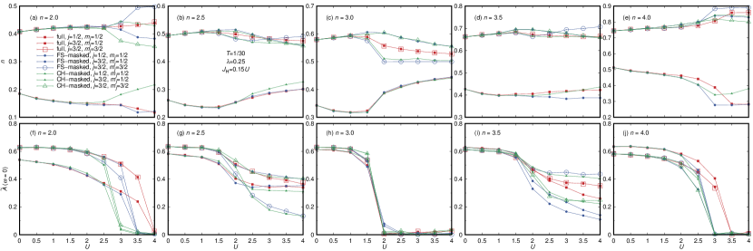
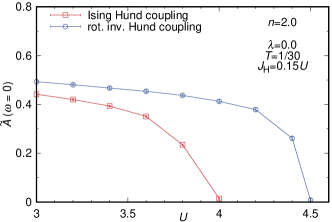
Such a modified degeneracy of the local Hamiltonian leads to substantial changes in observables, especially when the system becomes localized. In Figs. 5(a), 5(c), and 5(e), for example, one can see a sizable difference between the electron densities from the full and masked local Hamiltonians for the large- $U$ Mott insulator. The degeneracy of the electron density between the $j=3/2$ , $m_{j}=\pm 1/2$ , and $m_{j}=\pm 3/2$ flavors is naturally broken for the masked Hamiltonian. Mott localization is signaled by the suppression of the spectral function at the Fermi level, and this quantity can be approximately evaluated as $\tilde{A}(\omega=0)=-\frac{1}{\pi T}G(\tau=\beta/2)$ . Moreover, the Mott transition point $U_{c}$ for $n=2$ and $4$ is reduced as we mask the CH or FS terms. Compared to the FS-dropped Hamiltonian, the CH-dropped one shows a further reduction in $U_{c}$ for the $n=2$ case. This kind of $U_{c}$ reduction as a result of a degeneracy breaking was reported in a non-spin-orbit-coupled system in the presence of a single-particle crystal-field splitting Werner et al. (2009); Huang et al. (2012) and in the absence of the spin-flip and pair-hopping terms (so-called Ising-type Hund coupling) at the many-body level Huang et al. (2012) (see Fig. 6).

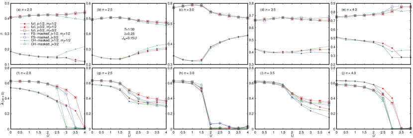
One interesting observation is that the density values of the full Hamiltonian are approximately recovered by the masked one if we artificially symmetrize the $j=3/2$ , $m_{j}=\pm 1/2$ , and $m_{j}=\pm 3/2$ flavors during the self-consistency loop of the DMFT. Figure 7 shows the corresponding electron density and the approximated spectral function at the Fermi level. The density values become much closer to those of the full Hamiltonian. Especially, the FS-dropped Hamiltonian at and below half-filling yields results which are consistent within $\sim 5\%$ relative error. As a result of the modification of the Hamiltonian, the sign problem of the CTHYB simulation is alleviated by up to $\sim 15\%$ . When applied with proper care, this symmetrization trick could provide a useful estimate for physical observables when the original Hamiltonian cannot be treated due to the serious sign problem.

$N$	$J_{z}$	Ground State
2	+2	$\alpha_{2}\left\|\leavevmode\hbox to28.85pt{\vbox to16.33pt{\pgfpicture\makeatletter\hbox{\hskip 0.2pt\lower-1.90709pt\hbox to0.0pt{\pgfsys@beginscope\pgfsys@invoke{ }\definecolor{pgfstrokecolor}{rgb}{0,0,0}\pgfsys@color@rgb@stroke{0}{0}{0}\pgfsys@invoke{ }\pgfsys@color@rgb@fill{0}{0}{0}\pgfsys@invoke{ }\pgfsys@setlinewidth{0.4pt}\pgfsys@invoke{ }\nullfont\hbox to0.0pt{\pgfsys@beginscope\pgfsys@invoke{ } {}{{}}{} {}{}{}\pgfsys@moveto{8.5359pt}{14.22638pt}\pgfsys@lineto{19.91684pt}{14.22638pt}\pgfsys@stroke\pgfsys@invoke{ } {}{{}}{} {}{}{}\pgfsys@moveto{0.0pt}{0.0pt}\pgfsys@lineto{11.38092pt}{0.0pt}\pgfsys@stroke\pgfsys@invoke{ } {}{{}}{} {}{}{}\pgfsys@moveto{17.07182pt}{0.0pt}\pgfsys@lineto{28.45276pt}{0.0pt}\pgfsys@stroke\pgfsys@invoke{ } {}{{}}{}{{{}}{}{}{}{}{}{}{}{}}{}\pgfsys@moveto{2.84544pt}{0.0pt}\pgfsys@moveto{4.55254pt}{0.0pt}\pgfsys@curveto{4.55254pt}{0.94281pt}{3.78825pt}{1.70709pt}{2.84544pt}{1.70709pt}\pgfsys@curveto{1.90263pt}{1.70709pt}{1.13835pt}{0.94281pt}{1.13835pt}{0.0pt}\pgfsys@curveto{1.13835pt}{-0.94281pt}{1.90263pt}{-1.70709pt}{2.84544pt}{-1.70709pt}\pgfsys@curveto{3.78825pt}{-1.70709pt}{4.55254pt}{-0.94281pt}{4.55254pt}{0.0pt}\pgfsys@closepath\pgfsys@moveto{2.84544pt}{0.0pt}\pgfsys@fillstroke\pgfsys@invoke{ } {}{{}}{}{{{}}{}{}{}{}{}{}{}{}}{}\pgfsys@moveto{19.91684pt}{0.0pt}\pgfsys@moveto{21.62393pt}{0.0pt}\pgfsys@curveto{21.62393pt}{0.94281pt}{20.85965pt}{1.70709pt}{19.91684pt}{1.70709pt}\pgfsys@curveto{18.97403pt}{1.70709pt}{18.20975pt}{0.94281pt}{18.20975pt}{0.0pt}\pgfsys@curveto{18.20975pt}{-0.94281pt}{18.97403pt}{-1.70709pt}{19.91684pt}{-1.70709pt}\pgfsys@curveto{20.85965pt}{-1.70709pt}{21.62393pt}{-0.94281pt}{21.62393pt}{0.0pt}\pgfsys@closepath\pgfsys@moveto{19.91684pt}{0.0pt}\pgfsys@fillstroke\pgfsys@invoke{ } {{}}\hbox{\hbox{{\pgfsys@beginscope\pgfsys@invoke{ }{{}{}{{ {}{}}}{ {}{}} {{}{{}}}{{}{}}{}{{}{}} { }{{{{}}\pgfsys@beginscope\pgfsys@invoke{ }\pgfsys@transformcm{1.0}{0.0}{0.0}{1.0}{11.38092pt}{5.69046pt}\pgfsys@invoke{ }\hbox{{\definecolor{pgfstrokecolor}{rgb}{0,0,0}\pgfsys@color@rgb@stroke{0}{0}{0}\pgfsys@invoke{ }\pgfsys@color@rgb@fill{0}{0}{0}\pgfsys@invoke{ }\hbox{} }}\pgfsys@invoke{\lxSVG@closescope }\pgfsys@endscope}}} \pgfsys@invoke{\lxSVG@closescope }\pgfsys@endscope}}} \pgfsys@invoke{\lxSVG@closescope }\pgfsys@endscope{{ {}{}{}}}{}{}\hss}\pgfsys@discardpath\pgfsys@invoke{\lxSVG@closescope }\pgfsys@endscope\hss}}\lxSVG@closescope\endpgfpicture}}\right\rangle-\beta_{2}\left\|\leavevmode\hbox to28.85pt{\vbox to18.04pt{\pgfpicture\makeatletter\hbox{\hskip 0.2pt\lower-1.90709pt\hbox to0.0pt{\pgfsys@beginscope\pgfsys@invoke{ }\definecolor{pgfstrokecolor}{rgb}{0,0,0}\pgfsys@color@rgb@stroke{0}{0}{0}\pgfsys@invoke{ }\pgfsys@color@rgb@fill{0}{0}{0}\pgfsys@invoke{ }\pgfsys@setlinewidth{0.4pt}\pgfsys@invoke{ }\nullfont\hbox to0.0pt{\pgfsys@beginscope\pgfsys@invoke{ } {}{{}}{} {}{}{}\pgfsys@moveto{8.5359pt}{14.22638pt}\pgfsys@lineto{19.91684pt}{14.22638pt}\pgfsys@stroke\pgfsys@invoke{ } {}{{}}{} {}{}{}\pgfsys@moveto{0.0pt}{0.0pt}\pgfsys@lineto{11.38092pt}{0.0pt}\pgfsys@stroke\pgfsys@invoke{ } {}{{}}{} {}{}{}\pgfsys@moveto{17.07182pt}{0.0pt}\pgfsys@lineto{28.45276pt}{0.0pt}\pgfsys@stroke\pgfsys@invoke{ } {}{{}}{}{{{}}{}{}{}{}{}{}{}{}}{}\pgfsys@moveto{11.38092pt}{14.22638pt}\pgfsys@moveto{13.08801pt}{14.22638pt}\pgfsys@curveto{13.08801pt}{15.16919pt}{12.32373pt}{15.93347pt}{11.38092pt}{15.93347pt}\pgfsys@curveto{10.43811pt}{15.93347pt}{9.67383pt}{15.16919pt}{9.67383pt}{14.22638pt}\pgfsys@curveto{9.67383pt}{13.28357pt}{10.43811pt}{12.51929pt}{11.38092pt}{12.51929pt}\pgfsys@curveto{12.32373pt}{12.51929pt}{13.08801pt}{13.28357pt}{13.08801pt}{14.22638pt}\pgfsys@closepath\pgfsys@moveto{11.38092pt}{14.22638pt}\pgfsys@fillstroke\pgfsys@invoke{ } {}{{}}{}{{{}}{}{}{}{}{}{}{}{}}{}\pgfsys@moveto{19.91684pt}{0.0pt}\pgfsys@moveto{21.62393pt}{0.0pt}\pgfsys@curveto{21.62393pt}{0.94281pt}{20.85965pt}{1.70709pt}{19.91684pt}{1.70709pt}\pgfsys@curveto{18.97403pt}{1.70709pt}{18.20975pt}{0.94281pt}{18.20975pt}{0.0pt}\pgfsys@curveto{18.20975pt}{-0.94281pt}{18.97403pt}{-1.70709pt}{19.91684pt}{-1.70709pt}\pgfsys@curveto{20.85965pt}{-1.70709pt}{21.62393pt}{-0.94281pt}{21.62393pt}{0.0pt}\pgfsys@closepath\pgfsys@moveto{19.91684pt}{0.0pt}\pgfsys@fillstroke\pgfsys@invoke{ } {{}}\hbox{\hbox{{\pgfsys@beginscope\pgfsys@invoke{ }{{}{}{{ {}{}}}{ {}{}} {{}{{}}}{{}{}}{}{{}{}} { }{{{{}}\pgfsys@beginscope\pgfsys@invoke{ }\pgfsys@transformcm{1.0}{0.0}{0.0}{1.0}{11.38092pt}{5.69046pt}\pgfsys@invoke{ }\hbox{{\definecolor{pgfstrokecolor}{rgb}{0,0,0}\pgfsys@color@rgb@stroke{0}{0}{0}\pgfsys@invoke{ }\pgfsys@color@rgb@fill{0}{0}{0}\pgfsys@invoke{ }\hbox{} }}\pgfsys@invoke{\lxSVG@closescope }\pgfsys@endscope}}} \pgfsys@invoke{\lxSVG@closescope }\pgfsys@endscope}}} \pgfsys@invoke{\lxSVG@closescope }\pgfsys@endscope{{ {}{}{}}}{}{}\hss}\pgfsys@discardpath\pgfsys@invoke{\lxSVG@closescope }\pgfsys@endscope\hss}}\lxSVG@closescope\endpgfpicture}}\right\rangle$
	+1	$\alpha_{2}^{\prime}\left\|\leavevmode\hbox to28.85pt{\vbox to16.33pt{\pgfpicture\makeatletter\hbox{\hskip 0.2pt\lower-1.90709pt\hbox to0.0pt{\pgfsys@beginscope\pgfsys@invoke{ }\definecolor{pgfstrokecolor}{rgb}{0,0,0}\pgfsys@color@rgb@stroke{0}{0}{0}\pgfsys@invoke{ }\pgfsys@color@rgb@fill{0}{0}{0}\pgfsys@invoke{ }\pgfsys@setlinewidth{0.4pt}\pgfsys@invoke{ }\nullfont\hbox to0.0pt{\pgfsys@beginscope\pgfsys@invoke{ } {}{{}}{} {}{}{}\pgfsys@moveto{8.5359pt}{14.22638pt}\pgfsys@lineto{19.91684pt}{14.22638pt}\pgfsys@stroke\pgfsys@invoke{ } {}{{}}{} {}{}{}\pgfsys@moveto{0.0pt}{0.0pt}\pgfsys@lineto{11.38092pt}{0.0pt}\pgfsys@stroke\pgfsys@invoke{ } {}{{}}{} {}{}{}\pgfsys@moveto{17.07182pt}{0.0pt}\pgfsys@lineto{28.45276pt}{0.0pt}\pgfsys@stroke\pgfsys@invoke{ } {}{{}}{}{{{}}{}{}{}{}{}{}{}{}}{}\pgfsys@moveto{19.91684pt}{0.0pt}\pgfsys@moveto{21.62393pt}{0.0pt}\pgfsys@curveto{21.62393pt}{0.94281pt}{20.85965pt}{1.70709pt}{19.91684pt}{1.70709pt}\pgfsys@curveto{18.97403pt}{1.70709pt}{18.20975pt}{0.94281pt}{18.20975pt}{0.0pt}\pgfsys@curveto{18.20975pt}{-0.94281pt}{18.97403pt}{-1.70709pt}{19.91684pt}{-1.70709pt}\pgfsys@curveto{20.85965pt}{-1.70709pt}{21.62393pt}{-0.94281pt}{21.62393pt}{0.0pt}\pgfsys@closepath\pgfsys@moveto{19.91684pt}{0.0pt}\pgfsys@fillstroke\pgfsys@invoke{ } {}{{}}{}{{{}}{}{}{}{}{}{}{}{}}{}\pgfsys@moveto{8.5359pt}{0.0pt}\pgfsys@moveto{10.243pt}{0.0pt}\pgfsys@curveto{10.243pt}{0.94281pt}{9.47871pt}{1.70709pt}{8.5359pt}{1.70709pt}\pgfsys@curveto{7.5931pt}{1.70709pt}{6.82881pt}{0.94281pt}{6.82881pt}{0.0pt}\pgfsys@curveto{6.82881pt}{-0.94281pt}{7.5931pt}{-1.70709pt}{8.5359pt}{-1.70709pt}\pgfsys@curveto{9.47871pt}{-1.70709pt}{10.243pt}{-0.94281pt}{10.243pt}{0.0pt}\pgfsys@closepath\pgfsys@moveto{8.5359pt}{0.0pt}\pgfsys@stroke\pgfsys@invoke{ } {{}}\hbox{\hbox{{\pgfsys@beginscope\pgfsys@invoke{ }{{}{}{{ {}{}}}{ {}{}} {{}{{}}}{{}{}}{}{{}{}} { }{{{{}}\pgfsys@beginscope\pgfsys@invoke{ }\pgfsys@transformcm{1.0}{0.0}{0.0}{1.0}{11.38092pt}{5.69046pt}\pgfsys@invoke{ }\hbox{{\definecolor{pgfstrokecolor}{rgb}{0,0,0}\pgfsys@color@rgb@stroke{0}{0}{0}\pgfsys@invoke{ }\pgfsys@color@rgb@fill{0}{0}{0}\pgfsys@invoke{ }\hbox{} }}\pgfsys@invoke{\lxSVG@closescope }\pgfsys@endscope}}} \pgfsys@invoke{\lxSVG@closescope }\pgfsys@endscope}}} \pgfsys@invoke{\lxSVG@closescope }\pgfsys@endscope{{ {}{}{}}}{}{}\hss}\pgfsys@discardpath\pgfsys@invoke{\lxSVG@closescope }\pgfsys@endscope\hss}}\lxSVG@closescope\endpgfpicture}}\right\rangle-\beta_{2}^{\prime}\left\|\leavevmode\hbox to28.85pt{\vbox to18.04pt{\pgfpicture\makeatletter\hbox{\hskip 0.2pt\lower-1.90709pt\hbox to0.0pt{\pgfsys@beginscope\pgfsys@invoke{ }\definecolor{pgfstrokecolor}{rgb}{0,0,0}\pgfsys@color@rgb@stroke{0}{0}{0}\pgfsys@invoke{ }\pgfsys@color@rgb@fill{0}{0}{0}\pgfsys@invoke{ }\pgfsys@setlinewidth{0.4pt}\pgfsys@invoke{ }\nullfont\hbox to0.0pt{\pgfsys@beginscope\pgfsys@invoke{ } {}{{}}{} {}{}{}\pgfsys@moveto{8.5359pt}{14.22638pt}\pgfsys@lineto{19.91684pt}{14.22638pt}\pgfsys@stroke\pgfsys@invoke{ } {}{{}}{} {}{}{}\pgfsys@moveto{0.0pt}{0.0pt}\pgfsys@lineto{11.38092pt}{0.0pt}\pgfsys@stroke\pgfsys@invoke{ } {}{{}}{} {}{}{}\pgfsys@moveto{17.07182pt}{0.0pt}\pgfsys@lineto{28.45276pt}{0.0pt}\pgfsys@stroke\pgfsys@invoke{ } {}{{}}{}{{{}}{}{}{}{}{}{}{}{}}{}\pgfsys@moveto{11.38092pt}{14.22638pt}\pgfsys@moveto{13.08801pt}{14.22638pt}\pgfsys@curveto{13.08801pt}{15.16919pt}{12.32373pt}{15.93347pt}{11.38092pt}{15.93347pt}\pgfsys@curveto{10.43811pt}{15.93347pt}{9.67383pt}{15.16919pt}{9.67383pt}{14.22638pt}\pgfsys@curveto{9.67383pt}{13.28357pt}{10.43811pt}{12.51929pt}{11.38092pt}{12.51929pt}\pgfsys@curveto{12.32373pt}{12.51929pt}{13.08801pt}{13.28357pt}{13.08801pt}{14.22638pt}\pgfsys@closepath\pgfsys@moveto{11.38092pt}{14.22638pt}\pgfsys@fillstroke\pgfsys@invoke{ } {}{{}}{}{{{}}{}{}{}{}{}{}{}{}}{}\pgfsys@moveto{2.84544pt}{0.0pt}\pgfsys@moveto{4.55254pt}{0.0pt}\pgfsys@curveto{4.55254pt}{0.94281pt}{3.78825pt}{1.70709pt}{2.84544pt}{1.70709pt}\pgfsys@curveto{1.90263pt}{1.70709pt}{1.13835pt}{0.94281pt}{1.13835pt}{0.0pt}\pgfsys@curveto{1.13835pt}{-0.94281pt}{1.90263pt}{-1.70709pt}{2.84544pt}{-1.70709pt}\pgfsys@curveto{3.78825pt}{-1.70709pt}{4.55254pt}{-0.94281pt}{4.55254pt}{0.0pt}\pgfsys@closepath\pgfsys@moveto{2.84544pt}{0.0pt}\pgfsys@fillstroke\pgfsys@invoke{ } {{}}\hbox{\hbox{{\pgfsys@beginscope\pgfsys@invoke{ }{{}{}{{ {}{}}}{ {}{}} {{}{{}}}{{}{}}{}{{}{}} { }{{{{}}\pgfsys@beginscope\pgfsys@invoke{ }\pgfsys@transformcm{1.0}{0.0}{0.0}{1.0}{11.38092pt}{5.69046pt}\pgfsys@invoke{ }\hbox{{\definecolor{pgfstrokecolor}{rgb}{0,0,0}\pgfsys@color@rgb@stroke{0}{0}{0}\pgfsys@invoke{ }\pgfsys@color@rgb@fill{0}{0}{0}\pgfsys@invoke{ }\hbox{} }}\pgfsys@invoke{\lxSVG@closescope }\pgfsys@endscope}}} \pgfsys@invoke{\lxSVG@closescope }\pgfsys@endscope}}} \pgfsys@invoke{\lxSVG@closescope }\pgfsys@endscope{{ {}{}{}}}{}{}\hss}\pgfsys@discardpath\pgfsys@invoke{\lxSVG@closescope }\pgfsys@endscope\hss}}\lxSVG@closescope\endpgfpicture}}\right\rangle-\gamma_{2}^{\prime}\left\|\leavevmode\hbox to28.85pt{\vbox to18.04pt{\pgfpicture\makeatletter\hbox{\hskip 0.2pt\lower-1.90709pt\hbox to0.0pt{\pgfsys@beginscope\pgfsys@invoke{ }\definecolor{pgfstrokecolor}{rgb}{0,0,0}\pgfsys@color@rgb@stroke{0}{0}{0}\pgfsys@invoke{ }\pgfsys@color@rgb@fill{0}{0}{0}\pgfsys@invoke{ }\pgfsys@setlinewidth{0.4pt}\pgfsys@invoke{ }\nullfont\hbox to0.0pt{\pgfsys@beginscope\pgfsys@invoke{ } {}{{}}{} {}{}{}\pgfsys@moveto{8.5359pt}{14.22638pt}\pgfsys@lineto{19.91684pt}{14.22638pt}\pgfsys@stroke\pgfsys@invoke{ } {}{{}}{} {}{}{}\pgfsys@moveto{0.0pt}{0.0pt}\pgfsys@lineto{11.38092pt}{0.0pt}\pgfsys@stroke\pgfsys@invoke{ } {}{{}}{} {}{}{}\pgfsys@moveto{17.07182pt}{0.0pt}\pgfsys@lineto{28.45276pt}{0.0pt}\pgfsys@stroke\pgfsys@invoke{ } {}{{}}{}{{{}}{}{}{}{}{}{}{}{}}{}\pgfsys@moveto{19.91684pt}{0.0pt}\pgfsys@moveto{21.62393pt}{0.0pt}\pgfsys@curveto{21.62393pt}{0.94281pt}{20.85965pt}{1.70709pt}{19.91684pt}{1.70709pt}\pgfsys@curveto{18.97403pt}{1.70709pt}{18.20975pt}{0.94281pt}{18.20975pt}{0.0pt}\pgfsys@curveto{18.20975pt}{-0.94281pt}{18.97403pt}{-1.70709pt}{19.91684pt}{-1.70709pt}\pgfsys@curveto{20.85965pt}{-1.70709pt}{21.62393pt}{-0.94281pt}{21.62393pt}{0.0pt}\pgfsys@closepath\pgfsys@moveto{19.91684pt}{0.0pt}\pgfsys@fillstroke\pgfsys@invoke{ } {}{{}}{}{{{}}{}{}{}{}{}{}{}{}}{}\pgfsys@moveto{17.07182pt}{14.22638pt}\pgfsys@moveto{18.77892pt}{14.22638pt}\pgfsys@curveto{18.77892pt}{15.16919pt}{18.01463pt}{15.93347pt}{17.07182pt}{15.93347pt}\pgfsys@curveto{16.12901pt}{15.93347pt}{15.36473pt}{15.16919pt}{15.36473pt}{14.22638pt}\pgfsys@curveto{15.36473pt}{13.28357pt}{16.12901pt}{12.51929pt}{17.07182pt}{12.51929pt}\pgfsys@curveto{18.01463pt}{12.51929pt}{18.77892pt}{13.28357pt}{18.77892pt}{14.22638pt}\pgfsys@closepath\pgfsys@moveto{17.07182pt}{14.22638pt}\pgfsys@stroke\pgfsys@invoke{ } {{}}\hbox{\hbox{{\pgfsys@beginscope\pgfsys@invoke{ }{{}{}{{ {}{}}}{ {}{}} {{}{{}}}{{}{}}{}{{}{}} { }{{{{}}\pgfsys@beginscope\pgfsys@invoke{ }\pgfsys@transformcm{1.0}{0.0}{0.0}{1.0}{11.38092pt}{5.69046pt}\pgfsys@invoke{ }\hbox{{\definecolor{pgfstrokecolor}{rgb}{0,0,0}\pgfsys@color@rgb@stroke{0}{0}{0}\pgfsys@invoke{ }\pgfsys@color@rgb@fill{0}{0}{0}\pgfsys@invoke{ }\hbox{} }}\pgfsys@invoke{\lxSVG@closescope }\pgfsys@endscope}}} \pgfsys@invoke{\lxSVG@closescope }\pgfsys@endscope}}} \pgfsys@invoke{\lxSVG@closescope }\pgfsys@endscope{{ {}{}{}}}{}{}\hss}\pgfsys@discardpath\pgfsys@invoke{\lxSVG@closescope }\pgfsys@endscope\hss}}\lxSVG@closescope\endpgfpicture}}\right\rangle$
	0	$\alpha_{2}^{\prime\prime}\left(\left\|\leavevmode\hbox to28.85pt{\vbox to16.33pt{\pgfpicture\makeatletter\hbox{\hskip 0.2pt\lower-1.90709pt\hbox to0.0pt{\pgfsys@beginscope\pgfsys@invoke{ }\definecolor{pgfstrokecolor}{rgb}{0,0,0}\pgfsys@color@rgb@stroke{0}{0}{0}\pgfsys@invoke{ }\pgfsys@color@rgb@fill{0}{0}{0}\pgfsys@invoke{ }\pgfsys@setlinewidth{0.4pt}\pgfsys@invoke{ }\nullfont\hbox to0.0pt{\pgfsys@beginscope\pgfsys@invoke{ } {}{{}}{} {}{}{}\pgfsys@moveto{8.5359pt}{14.22638pt}\pgfsys@lineto{19.91684pt}{14.22638pt}\pgfsys@stroke\pgfsys@invoke{ } {}{{}}{} {}{}{}\pgfsys@moveto{0.0pt}{0.0pt}\pgfsys@lineto{11.38092pt}{0.0pt}\pgfsys@stroke\pgfsys@invoke{ } {}{{}}{} {}{}{}\pgfsys@moveto{17.07182pt}{0.0pt}\pgfsys@lineto{28.45276pt}{0.0pt}\pgfsys@stroke\pgfsys@invoke{ } {}{{}}{}{{{}}{}{}{}{}{}{}{}{}}{}\pgfsys@moveto{2.84544pt}{0.0pt}\pgfsys@moveto{4.55254pt}{0.0pt}\pgfsys@curveto{4.55254pt}{0.94281pt}{3.78825pt}{1.70709pt}{2.84544pt}{1.70709pt}\pgfsys@curveto{1.90263pt}{1.70709pt}{1.13835pt}{0.94281pt}{1.13835pt}{0.0pt}\pgfsys@curveto{1.13835pt}{-0.94281pt}{1.90263pt}{-1.70709pt}{2.84544pt}{-1.70709pt}\pgfsys@curveto{3.78825pt}{-1.70709pt}{4.55254pt}{-0.94281pt}{4.55254pt}{0.0pt}\pgfsys@closepath\pgfsys@moveto{2.84544pt}{0.0pt}\pgfsys@fillstroke\pgfsys@invoke{ } {}{{}}{}{{{}}{}{}{}{}{}{}{}{}}{}\pgfsys@moveto{8.5359pt}{0.0pt}\pgfsys@moveto{10.243pt}{0.0pt}\pgfsys@curveto{10.243pt}{0.94281pt}{9.47871pt}{1.70709pt}{8.5359pt}{1.70709pt}\pgfsys@curveto{7.5931pt}{1.70709pt}{6.82881pt}{0.94281pt}{6.82881pt}{0.0pt}\pgfsys@curveto{6.82881pt}{-0.94281pt}{7.5931pt}{-1.70709pt}{8.5359pt}{-1.70709pt}\pgfsys@curveto{9.47871pt}{-1.70709pt}{10.243pt}{-0.94281pt}{10.243pt}{0.0pt}\pgfsys@closepath\pgfsys@moveto{8.5359pt}{0.0pt}\pgfsys@stroke\pgfsys@invoke{ } {{}}\hbox{\hbox{{\pgfsys@beginscope\pgfsys@invoke{ }{{}{}{{ {}{}}}{ {}{}} {{}{{}}}{{}{}}{}{{}{}} { }{{{{}}\pgfsys@beginscope\pgfsys@invoke{ }\pgfsys@transformcm{1.0}{0.0}{0.0}{1.0}{11.38092pt}{5.69046pt}\pgfsys@invoke{ }\hbox{{\definecolor{pgfstrokecolor}{rgb}{0,0,0}\pgfsys@color@rgb@stroke{0}{0}{0}\pgfsys@invoke{ }\pgfsys@color@rgb@fill{0}{0}{0}\pgfsys@invoke{ }\hbox{} }}\pgfsys@invoke{\lxSVG@closescope }\pgfsys@endscope}}} \pgfsys@invoke{\lxSVG@closescope }\pgfsys@endscope}}} \pgfsys@invoke{\lxSVG@closescope }\pgfsys@endscope{{ {}{}{}}}{}{}\hss}\pgfsys@discardpath\pgfsys@invoke{\lxSVG@closescope }\pgfsys@endscope\hss}}\lxSVG@closescope\endpgfpicture}}\right\rangle+\left\|\leavevmode\hbox to28.85pt{\vbox to16.33pt{\pgfpicture\makeatletter\hbox{\hskip 0.2pt\lower-1.90709pt\hbox to0.0pt{\pgfsys@beginscope\pgfsys@invoke{ }\definecolor{pgfstrokecolor}{rgb}{0,0,0}\pgfsys@color@rgb@stroke{0}{0}{0}\pgfsys@invoke{ }\pgfsys@color@rgb@fill{0}{0}{0}\pgfsys@invoke{ }\pgfsys@setlinewidth{0.4pt}\pgfsys@invoke{ }\nullfont\hbox to0.0pt{\pgfsys@beginscope\pgfsys@invoke{ } {}{{}}{} {}{}{}\pgfsys@moveto{8.5359pt}{14.22638pt}\pgfsys@lineto{19.91684pt}{14.22638pt}\pgfsys@stroke\pgfsys@invoke{ } {}{{}}{} {}{}{}\pgfsys@moveto{0.0pt}{0.0pt}\pgfsys@lineto{11.38092pt}{0.0pt}\pgfsys@stroke\pgfsys@invoke{ } {}{{}}{} {}{}{}\pgfsys@moveto{17.07182pt}{0.0pt}\pgfsys@lineto{28.45276pt}{0.0pt}\pgfsys@stroke\pgfsys@invoke{ } {}{{}}{}{{{}}{}{}{}{}{}{}{}{}}{}\pgfsys@moveto{19.91684pt}{0.0pt}\pgfsys@moveto{21.62393pt}{0.0pt}\pgfsys@curveto{21.62393pt}{0.94281pt}{20.85965pt}{1.70709pt}{19.91684pt}{1.70709pt}\pgfsys@curveto{18.97403pt}{1.70709pt}{18.20975pt}{0.94281pt}{18.20975pt}{0.0pt}\pgfsys@curveto{18.20975pt}{-0.94281pt}{18.97403pt}{-1.70709pt}{19.91684pt}{-1.70709pt}\pgfsys@curveto{20.85965pt}{-1.70709pt}{21.62393pt}{-0.94281pt}{21.62393pt}{0.0pt}\pgfsys@closepath\pgfsys@moveto{19.91684pt}{0.0pt}\pgfsys@fillstroke\pgfsys@invoke{ } {}{{}}{}{{{}}{}{}{}{}{}{}{}{}}{}\pgfsys@moveto{25.6073pt}{0.0pt}\pgfsys@moveto{27.31439pt}{0.0pt}\pgfsys@curveto{27.31439pt}{0.94281pt}{26.55011pt}{1.70709pt}{25.6073pt}{1.70709pt}\pgfsys@curveto{24.66449pt}{1.70709pt}{23.9002pt}{0.94281pt}{23.9002pt}{0.0pt}\pgfsys@curveto{23.9002pt}{-0.94281pt}{24.66449pt}{-1.70709pt}{25.6073pt}{-1.70709pt}\pgfsys@curveto{26.55011pt}{-1.70709pt}{27.31439pt}{-0.94281pt}{27.31439pt}{0.0pt}\pgfsys@closepath\pgfsys@moveto{25.6073pt}{0.0pt}\pgfsys@stroke\pgfsys@invoke{ } {{}}\hbox{\hbox{{\pgfsys@beginscope\pgfsys@invoke{ }{{}{}{{ {}{}}}{ {}{}} {{}{{}}}{{}{}}{}{{}{}} { }{{{{}}\pgfsys@beginscope\pgfsys@invoke{ }\pgfsys@transformcm{1.0}{0.0}{0.0}{1.0}{11.38092pt}{5.69046pt}\pgfsys@invoke{ }\hbox{{\definecolor{pgfstrokecolor}{rgb}{0,0,0}\pgfsys@color@rgb@stroke{0}{0}{0}\pgfsys@invoke{ }\pgfsys@color@rgb@fill{0}{0}{0}\pgfsys@invoke{ }\hbox{} }}\pgfsys@invoke{\lxSVG@closescope }\pgfsys@endscope}}} \pgfsys@invoke{\lxSVG@closescope }\pgfsys@endscope}}} \pgfsys@invoke{\lxSVG@closescope }\pgfsys@endscope{{ {}{}{}}}{}{}\hss}\pgfsys@discardpath\pgfsys@invoke{\lxSVG@closescope }\pgfsys@endscope\hss}}\lxSVG@closescope\endpgfpicture}}\right\rangle\right)+\beta_{2}^{\prime\prime}\left(\left\|\leavevmode\hbox to28.85pt{\vbox to18.04pt{\pgfpicture\makeatletter\hbox{\hskip 0.2pt\lower-1.90709pt\hbox to0.0pt{\pgfsys@beginscope\pgfsys@invoke{ }\definecolor{pgfstrokecolor}{rgb}{0,0,0}\pgfsys@color@rgb@stroke{0}{0}{0}\pgfsys@invoke{ }\pgfsys@color@rgb@fill{0}{0}{0}\pgfsys@invoke{ }\pgfsys@setlinewidth{0.4pt}\pgfsys@invoke{ }\nullfont\hbox to0.0pt{\pgfsys@beginscope\pgfsys@invoke{ } {}{{}}{} {}{}{}\pgfsys@moveto{8.5359pt}{14.22638pt}\pgfsys@lineto{19.91684pt}{14.22638pt}\pgfsys@stroke\pgfsys@invoke{ } {}{{}}{} {}{}{}\pgfsys@moveto{0.0pt}{0.0pt}\pgfsys@lineto{11.38092pt}{0.0pt}\pgfsys@stroke\pgfsys@invoke{ } {}{{}}{} {}{}{}\pgfsys@moveto{17.07182pt}{0.0pt}\pgfsys@lineto{28.45276pt}{0.0pt}\pgfsys@stroke\pgfsys@invoke{ } {}{{}}{}{{{}}{}{}{}{}{}{}{}{}}{}\pgfsys@moveto{11.38092pt}{14.22638pt}\pgfsys@moveto{13.08801pt}{14.22638pt}\pgfsys@curveto{13.08801pt}{15.16919pt}{12.32373pt}{15.93347pt}{11.38092pt}{15.93347pt}\pgfsys@curveto{10.43811pt}{15.93347pt}{9.67383pt}{15.16919pt}{9.67383pt}{14.22638pt}\pgfsys@curveto{9.67383pt}{13.28357pt}{10.43811pt}{12.51929pt}{11.38092pt}{12.51929pt}\pgfsys@curveto{12.32373pt}{12.51929pt}{13.08801pt}{13.28357pt}{13.08801pt}{14.22638pt}\pgfsys@closepath\pgfsys@moveto{11.38092pt}{14.22638pt}\pgfsys@fillstroke\pgfsys@invoke{ } {}{{}}{}{{{}}{}{}{}{}{}{}{}{}}{}\pgfsys@moveto{8.5359pt}{0.0pt}\pgfsys@moveto{10.243pt}{0.0pt}\pgfsys@curveto{10.243pt}{0.94281pt}{9.47871pt}{1.70709pt}{8.5359pt}{1.70709pt}\pgfsys@curveto{7.5931pt}{1.70709pt}{6.82881pt}{0.94281pt}{6.82881pt}{0.0pt}\pgfsys@curveto{6.82881pt}{-0.94281pt}{7.5931pt}{-1.70709pt}{8.5359pt}{-1.70709pt}\pgfsys@curveto{9.47871pt}{-1.70709pt}{10.243pt}{-0.94281pt}{10.243pt}{0.0pt}\pgfsys@closepath\pgfsys@moveto{8.5359pt}{0.0pt}\pgfsys@stroke\pgfsys@invoke{ } {{}}\hbox{\hbox{{\pgfsys@beginscope\pgfsys@invoke{ }{{}{}{{ {}{}}}{ {}{}} {{}{{}}}{{}{}}{}{{}{}} { }{{{{}}\pgfsys@beginscope\pgfsys@invoke{ }\pgfsys@transformcm{1.0}{0.0}{0.0}{1.0}{11.38092pt}{5.69046pt}\pgfsys@invoke{ }\hbox{{\definecolor{pgfstrokecolor}{rgb}{0,0,0}\pgfsys@color@rgb@stroke{0}{0}{0}\pgfsys@invoke{ }\pgfsys@color@rgb@fill{0}{0}{0}\pgfsys@invoke{ }\hbox{} }}\pgfsys@invoke{\lxSVG@closescope }\pgfsys@endscope}}} \pgfsys@invoke{\lxSVG@closescope }\pgfsys@endscope}}} \pgfsys@invoke{\lxSVG@closescope }\pgfsys@endscope{{ {}{}{}}}{}{}\hss}\pgfsys@discardpath\pgfsys@invoke{\lxSVG@closescope }\pgfsys@endscope\hss}}\lxSVG@closescope\endpgfpicture}}\right\rangle-\left\|\leavevmode\hbox to28.85pt{\vbox to18.04pt{\pgfpicture\makeatletter\hbox{\hskip 0.2pt\lower-1.90709pt\hbox to0.0pt{\pgfsys@beginscope\pgfsys@invoke{ }\definecolor{pgfstrokecolor}{rgb}{0,0,0}\pgfsys@color@rgb@stroke{0}{0}{0}\pgfsys@invoke{ }\pgfsys@color@rgb@fill{0}{0}{0}\pgfsys@invoke{ }\pgfsys@setlinewidth{0.4pt}\pgfsys@invoke{ }\nullfont\hbox to0.0pt{\pgfsys@beginscope\pgfsys@invoke{ } {}{{}}{} {}{}{}\pgfsys@moveto{8.5359pt}{14.22638pt}\pgfsys@lineto{19.91684pt}{14.22638pt}\pgfsys@stroke\pgfsys@invoke{ } {}{{}}{} {}{}{}\pgfsys@moveto{0.0pt}{0.0pt}\pgfsys@lineto{11.38092pt}{0.0pt}\pgfsys@stroke\pgfsys@invoke{ } {}{{}}{} {}{}{}\pgfsys@moveto{17.07182pt}{0.0pt}\pgfsys@lineto{28.45276pt}{0.0pt}\pgfsys@stroke\pgfsys@invoke{ } {}{{}}{}{{{}}{}{}{}{}{}{}{}{}}{}\pgfsys@moveto{2.84544pt}{0.0pt}\pgfsys@moveto{4.55254pt}{0.0pt}\pgfsys@curveto{4.55254pt}{0.94281pt}{3.78825pt}{1.70709pt}{2.84544pt}{1.70709pt}\pgfsys@curveto{1.90263pt}{1.70709pt}{1.13835pt}{0.94281pt}{1.13835pt}{0.0pt}\pgfsys@curveto{1.13835pt}{-0.94281pt}{1.90263pt}{-1.70709pt}{2.84544pt}{-1.70709pt}\pgfsys@curveto{3.78825pt}{-1.70709pt}{4.55254pt}{-0.94281pt}{4.55254pt}{0.0pt}\pgfsys@closepath\pgfsys@moveto{2.84544pt}{0.0pt}\pgfsys@fillstroke\pgfsys@invoke{ } {}{{}}{}{{{}}{}{}{}{}{}{}{}{}}{}\pgfsys@moveto{17.07182pt}{14.22638pt}\pgfsys@moveto{18.77892pt}{14.22638pt}\pgfsys@curveto{18.77892pt}{15.16919pt}{18.01463pt}{15.93347pt}{17.07182pt}{15.93347pt}\pgfsys@curveto{16.12901pt}{15.93347pt}{15.36473pt}{15.16919pt}{15.36473pt}{14.22638pt}\pgfsys@curveto{15.36473pt}{13.28357pt}{16.12901pt}{12.51929pt}{17.07182pt}{12.51929pt}\pgfsys@curveto{18.01463pt}{12.51929pt}{18.77892pt}{13.28357pt}{18.77892pt}{14.22638pt}\pgfsys@closepath\pgfsys@moveto{17.07182pt}{14.22638pt}\pgfsys@stroke\pgfsys@invoke{ } {{}}\hbox{\hbox{{\pgfsys@beginscope\pgfsys@invoke{ }{{}{}{{ {}{}}}{ {}{}} {{}{{}}}{{}{}}{}{{}{}} { }{{{{}}\pgfsys@beginscope\pgfsys@invoke{ }\pgfsys@transformcm{1.0}{0.0}{0.0}{1.0}{11.38092pt}{5.69046pt}\pgfsys@invoke{ }\hbox{{\definecolor{pgfstrokecolor}{rgb}{0,0,0}\pgfsys@color@rgb@stroke{0}{0}{0}\pgfsys@invoke{ }\pgfsys@color@rgb@fill{0}{0}{0}\pgfsys@invoke{ }\hbox{} }}\pgfsys@invoke{\lxSVG@closescope }\pgfsys@endscope}}} \pgfsys@invoke{\lxSVG@closescope }\pgfsys@endscope}}} \pgfsys@invoke{\lxSVG@closescope }\pgfsys@endscope{{ {}{}{}}}{}{}\hss}\pgfsys@discardpath\pgfsys@invoke{\lxSVG@closescope }\pgfsys@endscope\hss}}\lxSVG@closescope\endpgfpicture}}\right\rangle\right)$
	-1	$\alpha_{2}^{\prime}\left\|\leavevmode\hbox to28.85pt{\vbox to16.33pt{\pgfpicture\makeatletter\hbox{\hskip 0.2pt\lower-1.90709pt\hbox to0.0pt{\pgfsys@beginscope\pgfsys@invoke{ }\definecolor{pgfstrokecolor}{rgb}{0,0,0}\pgfsys@color@rgb@stroke{0}{0}{0}\pgfsys@invoke{ }\pgfsys@color@rgb@fill{0}{0}{0}\pgfsys@invoke{ }\pgfsys@setlinewidth{0.4pt}\pgfsys@invoke{ }\nullfont\hbox to0.0pt{\pgfsys@beginscope\pgfsys@invoke{ } {}{{}}{} {}{}{}\pgfsys@moveto{8.5359pt}{14.22638pt}\pgfsys@lineto{19.91684pt}{14.22638pt}\pgfsys@stroke\pgfsys@invoke{ } {}{{}}{} {}{}{}\pgfsys@moveto{0.0pt}{0.0pt}\pgfsys@lineto{11.38092pt}{0.0pt}\pgfsys@stroke\pgfsys@invoke{ } {}{{}}{} {}{}{}\pgfsys@moveto{17.07182pt}{0.0pt}\pgfsys@lineto{28.45276pt}{0.0pt}\pgfsys@stroke\pgfsys@invoke{ } {}{{}}{}{{{}}{}{}{}{}{}{}{}{}}{}\pgfsys@moveto{2.84544pt}{0.0pt}\pgfsys@moveto{4.55254pt}{0.0pt}\pgfsys@curveto{4.55254pt}{0.94281pt}{3.78825pt}{1.70709pt}{2.84544pt}{1.70709pt}\pgfsys@curveto{1.90263pt}{1.70709pt}{1.13835pt}{0.94281pt}{1.13835pt}{0.0pt}\pgfsys@curveto{1.13835pt}{-0.94281pt}{1.90263pt}{-1.70709pt}{2.84544pt}{-1.70709pt}\pgfsys@curveto{3.78825pt}{-1.70709pt}{4.55254pt}{-0.94281pt}{4.55254pt}{0.0pt}\pgfsys@closepath\pgfsys@moveto{2.84544pt}{0.0pt}\pgfsys@fillstroke\pgfsys@invoke{ } {}{{}}{}{{{}}{}{}{}{}{}{}{}{}}{}\pgfsys@moveto{25.6073pt}{0.0pt}\pgfsys@moveto{27.31439pt}{0.0pt}\pgfsys@curveto{27.31439pt}{0.94281pt}{26.55011pt}{1.70709pt}{25.6073pt}{1.70709pt}\pgfsys@curveto{24.66449pt}{1.70709pt}{23.9002pt}{0.94281pt}{23.9002pt}{0.0pt}\pgfsys@curveto{23.9002pt}{-0.94281pt}{24.66449pt}{-1.70709pt}{25.6073pt}{-1.70709pt}\pgfsys@curveto{26.55011pt}{-1.70709pt}{27.31439pt}{-0.94281pt}{27.31439pt}{0.0pt}\pgfsys@closepath\pgfsys@moveto{25.6073pt}{0.0pt}\pgfsys@stroke\pgfsys@invoke{ } {{}}\hbox{\hbox{{\pgfsys@beginscope\pgfsys@invoke{ }{{}{}{{ {}{}}}{ {}{}} {{}{{}}}{{}{}}{}{{}{}} { }{{{{}}\pgfsys@beginscope\pgfsys@invoke{ }\pgfsys@transformcm{1.0}{0.0}{0.0}{1.0}{11.38092pt}{5.69046pt}\pgfsys@invoke{ }\hbox{{\definecolor{pgfstrokecolor}{rgb}{0,0,0}\pgfsys@color@rgb@stroke{0}{0}{0}\pgfsys@invoke{ }\pgfsys@color@rgb@fill{0}{0}{0}\pgfsys@invoke{ }\hbox{} }}\pgfsys@invoke{\lxSVG@closescope }\pgfsys@endscope}}} \pgfsys@invoke{\lxSVG@closescope }\pgfsys@endscope}}} \pgfsys@invoke{\lxSVG@closescope }\pgfsys@endscope{{ {}{}{}}}{}{}\hss}\pgfsys@discardpath\pgfsys@invoke{\lxSVG@closescope }\pgfsys@endscope\hss}}\lxSVG@closescope\endpgfpicture}}\right\rangle+\beta_{2}^{\prime}\left\|\leavevmode\hbox to28.85pt{\vbox to18.04pt{\pgfpicture\makeatletter\hbox{\hskip 0.2pt\lower-1.90709pt\hbox to0.0pt{\pgfsys@beginscope\pgfsys@invoke{ }\definecolor{pgfstrokecolor}{rgb}{0,0,0}\pgfsys@color@rgb@stroke{0}{0}{0}\pgfsys@invoke{ }\pgfsys@color@rgb@fill{0}{0}{0}\pgfsys@invoke{ }\pgfsys@setlinewidth{0.4pt}\pgfsys@invoke{ }\nullfont\hbox to0.0pt{\pgfsys@beginscope\pgfsys@invoke{ } {}{{}}{} {}{}{}\pgfsys@moveto{8.5359pt}{14.22638pt}\pgfsys@lineto{19.91684pt}{14.22638pt}\pgfsys@stroke\pgfsys@invoke{ } {}{{}}{} {}{}{}\pgfsys@moveto{0.0pt}{0.0pt}\pgfsys@lineto{11.38092pt}{0.0pt}\pgfsys@stroke\pgfsys@invoke{ } {}{{}}{} {}{}{}\pgfsys@moveto{17.07182pt}{0.0pt}\pgfsys@lineto{28.45276pt}{0.0pt}\pgfsys@stroke\pgfsys@invoke{ } {}{{}}{}{{{}}{}{}{}{}{}{}{}{}}{}\pgfsys@moveto{17.07182pt}{14.22638pt}\pgfsys@moveto{18.77892pt}{14.22638pt}\pgfsys@curveto{18.77892pt}{15.16919pt}{18.01463pt}{15.93347pt}{17.07182pt}{15.93347pt}\pgfsys@curveto{16.12901pt}{15.93347pt}{15.36473pt}{15.16919pt}{15.36473pt}{14.22638pt}\pgfsys@curveto{15.36473pt}{13.28357pt}{16.12901pt}{12.51929pt}{17.07182pt}{12.51929pt}\pgfsys@curveto{18.01463pt}{12.51929pt}{18.77892pt}{13.28357pt}{18.77892pt}{14.22638pt}\pgfsys@closepath\pgfsys@moveto{17.07182pt}{14.22638pt}\pgfsys@stroke\pgfsys@invoke{ } {}{{}}{}{{{}}{}{}{}{}{}{}{}{}}{}\pgfsys@moveto{8.5359pt}{0.0pt}\pgfsys@moveto{10.243pt}{0.0pt}\pgfsys@curveto{10.243pt}{0.94281pt}{9.47871pt}{1.70709pt}{8.5359pt}{1.70709pt}\pgfsys@curveto{7.5931pt}{1.70709pt}{6.82881pt}{0.94281pt}{6.82881pt}{0.0pt}\pgfsys@curveto{6.82881pt}{-0.94281pt}{7.5931pt}{-1.70709pt}{8.5359pt}{-1.70709pt}\pgfsys@curveto{9.47871pt}{-1.70709pt}{10.243pt}{-0.94281pt}{10.243pt}{0.0pt}\pgfsys@closepath\pgfsys@moveto{8.5359pt}{0.0pt}\pgfsys@stroke\pgfsys@invoke{ } {{}}\hbox{\hbox{{\pgfsys@beginscope\pgfsys@invoke{ }{{}{}{{ {}{}}}{ {}{}} {{}{{}}}{{}{}}{}{{}{}} { }{{{{}}\pgfsys@beginscope\pgfsys@invoke{ }\pgfsys@transformcm{1.0}{0.0}{0.0}{1.0}{11.38092pt}{5.69046pt}\pgfsys@invoke{ }\hbox{{\definecolor{pgfstrokecolor}{rgb}{0,0,0}\pgfsys@color@rgb@stroke{0}{0}{0}\pgfsys@invoke{ }\pgfsys@color@rgb@fill{0}{0}{0}\pgfsys@invoke{ }\hbox{} }}\pgfsys@invoke{\lxSVG@closescope }\pgfsys@endscope}}} \pgfsys@invoke{\lxSVG@closescope }\pgfsys@endscope}}} \pgfsys@invoke{\lxSVG@closescope }\pgfsys@endscope{{ {}{}{}}}{}{}\hss}\pgfsys@discardpath\pgfsys@invoke{\lxSVG@closescope }\pgfsys@endscope\hss}}\lxSVG@closescope\endpgfpicture}}\right\rangle+\gamma_{2}^{\prime}\left\|\leavevmode\hbox to28.85pt{\vbox to18.04pt{\pgfpicture\makeatletter\hbox{\hskip 0.2pt\lower-1.90709pt\hbox to0.0pt{\pgfsys@beginscope\pgfsys@invoke{ }\definecolor{pgfstrokecolor}{rgb}{0,0,0}\pgfsys@color@rgb@stroke{0}{0}{0}\pgfsys@invoke{ }\pgfsys@color@rgb@fill{0}{0}{0}\pgfsys@invoke{ }\pgfsys@setlinewidth{0.4pt}\pgfsys@invoke{ }\nullfont\hbox to0.0pt{\pgfsys@beginscope\pgfsys@invoke{ } {}{{}}{} {}{}{}\pgfsys@moveto{8.5359pt}{14.22638pt}\pgfsys@lineto{19.91684pt}{14.22638pt}\pgfsys@stroke\pgfsys@invoke{ } {}{{}}{} {}{}{}\pgfsys@moveto{0.0pt}{0.0pt}\pgfsys@lineto{11.38092pt}{0.0pt}\pgfsys@stroke\pgfsys@invoke{ } {}{{}}{} {}{}{}\pgfsys@moveto{17.07182pt}{0.0pt}\pgfsys@lineto{28.45276pt}{0.0pt}\pgfsys@stroke\pgfsys@invoke{ } {}{{}}{}{{{}}{}{}{}{}{}{}{}{}}{}\pgfsys@moveto{11.38092pt}{14.22638pt}\pgfsys@moveto{13.08801pt}{14.22638pt}\pgfsys@curveto{13.08801pt}{15.16919pt}{12.32373pt}{15.93347pt}{11.38092pt}{15.93347pt}\pgfsys@curveto{10.43811pt}{15.93347pt}{9.67383pt}{15.16919pt}{9.67383pt}{14.22638pt}\pgfsys@curveto{9.67383pt}{13.28357pt}{10.43811pt}{12.51929pt}{11.38092pt}{12.51929pt}\pgfsys@curveto{12.32373pt}{12.51929pt}{13.08801pt}{13.28357pt}{13.08801pt}{14.22638pt}\pgfsys@closepath\pgfsys@moveto{11.38092pt}{14.22638pt}\pgfsys@fillstroke\pgfsys@invoke{ } {}{{}}{}{{{}}{}{}{}{}{}{}{}{}}{}\pgfsys@moveto{25.6073pt}{0.0pt}\pgfsys@moveto{27.31439pt}{0.0pt}\pgfsys@curveto{27.31439pt}{0.94281pt}{26.55011pt}{1.70709pt}{25.6073pt}{1.70709pt}\pgfsys@curveto{24.66449pt}{1.70709pt}{23.9002pt}{0.94281pt}{23.9002pt}{0.0pt}\pgfsys@curveto{23.9002pt}{-0.94281pt}{24.66449pt}{-1.70709pt}{25.6073pt}{-1.70709pt}\pgfsys@curveto{26.55011pt}{-1.70709pt}{27.31439pt}{-0.94281pt}{27.31439pt}{0.0pt}\pgfsys@closepath\pgfsys@moveto{25.6073pt}{0.0pt}\pgfsys@stroke\pgfsys@invoke{ } {{}}\hbox{\hbox{{\pgfsys@beginscope\pgfsys@invoke{ }{{}{}{{ {}{}}}{ {}{}} {{}{{}}}{{}{}}{}{{}{}} { }{{{{}}\pgfsys@beginscope\pgfsys@invoke{ }\pgfsys@transformcm{1.0}{0.0}{0.0}{1.0}{11.38092pt}{5.69046pt}\pgfsys@invoke{ }\hbox{{\definecolor{pgfstrokecolor}{rgb}{0,0,0}\pgfsys@color@rgb@stroke{0}{0}{0}\pgfsys@invoke{ }\pgfsys@color@rgb@fill{0}{0}{0}\pgfsys@invoke{ }\hbox{} }}\pgfsys@invoke{\lxSVG@closescope }\pgfsys@endscope}}} \pgfsys@invoke{\lxSVG@closescope }\pgfsys@endscope}}} \pgfsys@invoke{\lxSVG@closescope }\pgfsys@endscope{{ {}{}{}}}{}{}\hss}\pgfsys@discardpath\pgfsys@invoke{\lxSVG@closescope }\pgfsys@endscope\hss}}\lxSVG@closescope\endpgfpicture}}\right\rangle$
	-2	$\alpha_{2}\left\|\leavevmode\hbox to28.85pt{\vbox to16.33pt{\pgfpicture\makeatletter\hbox{\hskip 0.2pt\lower-1.90709pt\hbox to0.0pt{\pgfsys@beginscope\pgfsys@invoke{ }\definecolor{pgfstrokecolor}{rgb}{0,0,0}\pgfsys@color@rgb@stroke{0}{0}{0}\pgfsys@invoke{ }\pgfsys@color@rgb@fill{0}{0}{0}\pgfsys@invoke{ }\pgfsys@setlinewidth{0.4pt}\pgfsys@invoke{ }\nullfont\hbox to0.0pt{\pgfsys@beginscope\pgfsys@invoke{ } {}{{}}{} {}{}{}\pgfsys@moveto{8.5359pt}{14.22638pt}\pgfsys@lineto{19.91684pt}{14.22638pt}\pgfsys@stroke\pgfsys@invoke{ } {}{{}}{} {}{}{}\pgfsys@moveto{0.0pt}{0.0pt}\pgfsys@lineto{11.38092pt}{0.0pt}\pgfsys@stroke\pgfsys@invoke{ } {}{{}}{} {}{}{}\pgfsys@moveto{17.07182pt}{0.0pt}\pgfsys@lineto{28.45276pt}{0.0pt}\pgfsys@stroke\pgfsys@invoke{ } {}{{}}{}{{{}}{}{}{}{}{}{}{}{}}{}\pgfsys@moveto{8.5359pt}{0.0pt}\pgfsys@moveto{10.243pt}{0.0pt}\pgfsys@curveto{10.243pt}{0.94281pt}{9.47871pt}{1.70709pt}{8.5359pt}{1.70709pt}\pgfsys@curveto{7.5931pt}{1.70709pt}{6.82881pt}{0.94281pt}{6.82881pt}{0.0pt}\pgfsys@curveto{6.82881pt}{-0.94281pt}{7.5931pt}{-1.70709pt}{8.5359pt}{-1.70709pt}\pgfsys@curveto{9.47871pt}{-1.70709pt}{10.243pt}{-0.94281pt}{10.243pt}{0.0pt}\pgfsys@closepath\pgfsys@moveto{8.5359pt}{0.0pt}\pgfsys@stroke\pgfsys@invoke{ } {}{{}}{}{{{}}{}{}{}{}{}{}{}{}}{}\pgfsys@moveto{25.6073pt}{0.0pt}\pgfsys@moveto{27.31439pt}{0.0pt}\pgfsys@curveto{27.31439pt}{0.94281pt}{26.55011pt}{1.70709pt}{25.6073pt}{1.70709pt}\pgfsys@curveto{24.66449pt}{1.70709pt}{23.9002pt}{0.94281pt}{23.9002pt}{0.0pt}\pgfsys@curveto{23.9002pt}{-0.94281pt}{24.66449pt}{-1.70709pt}{25.6073pt}{-1.70709pt}\pgfsys@curveto{26.55011pt}{-1.70709pt}{27.31439pt}{-0.94281pt}{27.31439pt}{0.0pt}\pgfsys@closepath\pgfsys@moveto{25.6073pt}{0.0pt}\pgfsys@stroke\pgfsys@invoke{ } {{}}\hbox{\hbox{{\pgfsys@beginscope\pgfsys@invoke{ }{{}{}{{ {}{}}}{ {}{}} {{}{{}}}{{}{}}{}{{}{}} { }{{{{}}\pgfsys@beginscope\pgfsys@invoke{ }\pgfsys@transformcm{1.0}{0.0}{0.0}{1.0}{11.38092pt}{5.69046pt}\pgfsys@invoke{ }\hbox{{\definecolor{pgfstrokecolor}{rgb}{0,0,0}\pgfsys@color@rgb@stroke{0}{0}{0}\pgfsys@invoke{ }\pgfsys@color@rgb@fill{0}{0}{0}\pgfsys@invoke{ }\hbox{} }}\pgfsys@invoke{\lxSVG@closescope }\pgfsys@endscope}}} \pgfsys@invoke{\lxSVG@closescope }\pgfsys@endscope}}} \pgfsys@invoke{\lxSVG@closescope }\pgfsys@endscope{{ {}{}{}}}{}{}\hss}\pgfsys@discardpath\pgfsys@invoke{\lxSVG@closescope }\pgfsys@endscope\hss}}\lxSVG@closescope\endpgfpicture}}\right\rangle+\beta_{2}\left\|\leavevmode\hbox to28.85pt{\vbox to18.04pt{\pgfpicture\makeatletter\hbox{\hskip 0.2pt\lower-1.90709pt\hbox to0.0pt{\pgfsys@beginscope\pgfsys@invoke{ }\definecolor{pgfstrokecolor}{rgb}{0,0,0}\pgfsys@color@rgb@stroke{0}{0}{0}\pgfsys@invoke{ }\pgfsys@color@rgb@fill{0}{0}{0}\pgfsys@invoke{ }\pgfsys@setlinewidth{0.4pt}\pgfsys@invoke{ }\nullfont\hbox to0.0pt{\pgfsys@beginscope\pgfsys@invoke{ } {}{{}}{} {}{}{}\pgfsys@moveto{8.5359pt}{14.22638pt}\pgfsys@lineto{19.91684pt}{14.22638pt}\pgfsys@stroke\pgfsys@invoke{ } {}{{}}{} {}{}{}\pgfsys@moveto{0.0pt}{0.0pt}\pgfsys@lineto{11.38092pt}{0.0pt}\pgfsys@stroke\pgfsys@invoke{ } {}{{}}{} {}{}{}\pgfsys@moveto{17.07182pt}{0.0pt}\pgfsys@lineto{28.45276pt}{0.0pt}\pgfsys@stroke\pgfsys@invoke{ } {}{{}}{}{{{}}{}{}{}{}{}{}{}{}}{}\pgfsys@moveto{17.07182pt}{14.22638pt}\pgfsys@moveto{18.77892pt}{14.22638pt}\pgfsys@curveto{18.77892pt}{15.16919pt}{18.01463pt}{15.93347pt}{17.07182pt}{15.93347pt}\pgfsys@curveto{16.12901pt}{15.93347pt}{15.36473pt}{15.16919pt}{15.36473pt}{14.22638pt}\pgfsys@curveto{15.36473pt}{13.28357pt}{16.12901pt}{12.51929pt}{17.07182pt}{12.51929pt}\pgfsys@curveto{18.01463pt}{12.51929pt}{18.77892pt}{13.28357pt}{18.77892pt}{14.22638pt}\pgfsys@closepath\pgfsys@moveto{17.07182pt}{14.22638pt}\pgfsys@stroke\pgfsys@invoke{ } {}{{}}{}{{{}}{}{}{}{}{}{}{}{}}{}\pgfsys@moveto{25.6073pt}{0.0pt}\pgfsys@moveto{27.31439pt}{0.0pt}\pgfsys@curveto{27.31439pt}{0.94281pt}{26.55011pt}{1.70709pt}{25.6073pt}{1.70709pt}\pgfsys@curveto{24.66449pt}{1.70709pt}{23.9002pt}{0.94281pt}{23.9002pt}{0.0pt}\pgfsys@curveto{23.9002pt}{-0.94281pt}{24.66449pt}{-1.70709pt}{25.6073pt}{-1.70709pt}\pgfsys@curveto{26.55011pt}{-1.70709pt}{27.31439pt}{-0.94281pt}{27.31439pt}{0.0pt}\pgfsys@closepath\pgfsys@moveto{25.6073pt}{0.0pt}\pgfsys@stroke\pgfsys@invoke{ } {{}}\hbox{\hbox{{\pgfsys@beginscope\pgfsys@invoke{ }{{}{}{{ {}{}}}{ {}{}} {{}{{}}}{{}{}}{}{{}{}} { }{{{{}}\pgfsys@beginscope\pgfsys@invoke{ }\pgfsys@transformcm{1.0}{0.0}{0.0}{1.0}{11.38092pt}{5.69046pt}\pgfsys@invoke{ }\hbox{{\definecolor{pgfstrokecolor}{rgb}{0,0,0}\pgfsys@color@rgb@stroke{0}{0}{0}\pgfsys@invoke{ }\pgfsys@color@rgb@fill{0}{0}{0}\pgfsys@invoke{ }\hbox{} }}\pgfsys@invoke{\lxSVG@closescope }\pgfsys@endscope}}} \pgfsys@invoke{\lxSVG@closescope }\pgfsys@endscope}}} \pgfsys@invoke{\lxSVG@closescope }\pgfsys@endscope{{ {}{}{}}}{}{}\hss}\pgfsys@discardpath\pgfsys@invoke{\lxSVG@closescope }\pgfsys@endscope\hss}}\lxSVG@closescope\endpgfpicture}}\right\rangle$
3	+3/2	$\alpha_{3}\left\|\leavevmode\hbox to28.85pt{\vbox to18.04pt{\pgfpicture\makeatletter\hbox{\hskip 0.2pt\lower-1.90709pt\hbox to0.0pt{\pgfsys@beginscope\pgfsys@invoke{ }\definecolor{pgfstrokecolor}{rgb}{0,0,0}\pgfsys@color@rgb@stroke{0}{0}{0}\pgfsys@invoke{ }\pgfsys@color@rgb@fill{0}{0}{0}\pgfsys@invoke{ }\pgfsys@setlinewidth{0.4pt}\pgfsys@invoke{ }\nullfont\hbox to0.0pt{\pgfsys@beginscope\pgfsys@invoke{ } {}{{}}{} {}{}{}\pgfsys@moveto{8.5359pt}{14.22638pt}\pgfsys@lineto{19.91684pt}{14.22638pt}\pgfsys@stroke\pgfsys@invoke{ } {}{{}}{} {}{}{}\pgfsys@moveto{0.0pt}{0.0pt}\pgfsys@lineto{11.38092pt}{0.0pt}\pgfsys@stroke\pgfsys@invoke{ } {}{{}}{} {}{}{}\pgfsys@moveto{17.07182pt}{0.0pt}\pgfsys@lineto{28.45276pt}{0.0pt}\pgfsys@stroke\pgfsys@invoke{ } {}{{}}{}{{{}}{}{}{}{}{}{}{}{}}{}\pgfsys@moveto{2.84544pt}{0.0pt}\pgfsys@moveto{4.55254pt}{0.0pt}\pgfsys@curveto{4.55254pt}{0.94281pt}{3.78825pt}{1.70709pt}{2.84544pt}{1.70709pt}\pgfsys@curveto{1.90263pt}{1.70709pt}{1.13835pt}{0.94281pt}{1.13835pt}{0.0pt}\pgfsys@curveto{1.13835pt}{-0.94281pt}{1.90263pt}{-1.70709pt}{2.84544pt}{-1.70709pt}\pgfsys@curveto{3.78825pt}{-1.70709pt}{4.55254pt}{-0.94281pt}{4.55254pt}{0.0pt}\pgfsys@closepath\pgfsys@moveto{2.84544pt}{0.0pt}\pgfsys@fillstroke\pgfsys@invoke{ } {}{{}}{}{{{}}{}{}{}{}{}{}{}{}}{}\pgfsys@moveto{19.91684pt}{0.0pt}\pgfsys@moveto{21.62393pt}{0.0pt}\pgfsys@curveto{21.62393pt}{0.94281pt}{20.85965pt}{1.70709pt}{19.91684pt}{1.70709pt}\pgfsys@curveto{18.97403pt}{1.70709pt}{18.20975pt}{0.94281pt}{18.20975pt}{0.0pt}\pgfsys@curveto{18.20975pt}{-0.94281pt}{18.97403pt}{-1.70709pt}{19.91684pt}{-1.70709pt}\pgfsys@curveto{20.85965pt}{-1.70709pt}{21.62393pt}{-0.94281pt}{21.62393pt}{0.0pt}\pgfsys@closepath\pgfsys@moveto{19.91684pt}{0.0pt}\pgfsys@fillstroke\pgfsys@invoke{ } {}{{}}{}{{{}}{}{}{}{}{}{}{}{}}{}\pgfsys@moveto{17.07182pt}{14.22638pt}\pgfsys@moveto{18.77892pt}{14.22638pt}\pgfsys@curveto{18.77892pt}{15.16919pt}{18.01463pt}{15.93347pt}{17.07182pt}{15.93347pt}\pgfsys@curveto{16.12901pt}{15.93347pt}{15.36473pt}{15.16919pt}{15.36473pt}{14.22638pt}\pgfsys@curveto{15.36473pt}{13.28357pt}{16.12901pt}{12.51929pt}{17.07182pt}{12.51929pt}\pgfsys@curveto{18.01463pt}{12.51929pt}{18.77892pt}{13.28357pt}{18.77892pt}{14.22638pt}\pgfsys@closepath\pgfsys@moveto{17.07182pt}{14.22638pt}\pgfsys@stroke\pgfsys@invoke{ } {{}}\hbox{\hbox{{\pgfsys@beginscope\pgfsys@invoke{ }{{}{}{{ {}{}}}{ {}{}} {{}{{}}}{{}{}}{}{{}{}} { }{{{{}}\pgfsys@beginscope\pgfsys@invoke{ }\pgfsys@transformcm{1.0}{0.0}{0.0}{1.0}{11.38092pt}{5.69046pt}\pgfsys@invoke{ }\hbox{{\definecolor{pgfstrokecolor}{rgb}{0,0,0}\pgfsys@color@rgb@stroke{0}{0}{0}\pgfsys@invoke{ }\pgfsys@color@rgb@fill{0}{0}{0}\pgfsys@invoke{ }\hbox{} }}\pgfsys@invoke{\lxSVG@closescope }\pgfsys@endscope}}} \pgfsys@invoke{\lxSVG@closescope }\pgfsys@endscope}}} \pgfsys@invoke{\lxSVG@closescope }\pgfsys@endscope{{ {}{}{}}}{}{}\hss}\pgfsys@discardpath\pgfsys@invoke{\lxSVG@closescope }\pgfsys@endscope\hss}}\lxSVG@closescope\endpgfpicture}}\right\rangle-\beta_{3}\left\|\leavevmode\hbox to28.85pt{\vbox to16.33pt{\pgfpicture\makeatletter\hbox{\hskip 0.2pt\lower-1.90709pt\hbox to0.0pt{\pgfsys@beginscope\pgfsys@invoke{ }\definecolor{pgfstrokecolor}{rgb}{0,0,0}\pgfsys@color@rgb@stroke{0}{0}{0}\pgfsys@invoke{ }\pgfsys@color@rgb@fill{0}{0}{0}\pgfsys@invoke{ }\pgfsys@setlinewidth{0.4pt}\pgfsys@invoke{ }\nullfont\hbox to0.0pt{\pgfsys@beginscope\pgfsys@invoke{ } {}{{}}{} {}{}{}\pgfsys@moveto{8.5359pt}{14.22638pt}\pgfsys@lineto{19.91684pt}{14.22638pt}\pgfsys@stroke\pgfsys@invoke{ } {}{{}}{} {}{}{}\pgfsys@moveto{0.0pt}{0.0pt}\pgfsys@lineto{11.38092pt}{0.0pt}\pgfsys@stroke\pgfsys@invoke{ } {}{{}}{} {}{}{}\pgfsys@moveto{17.07182pt}{0.0pt}\pgfsys@lineto{28.45276pt}{0.0pt}\pgfsys@stroke\pgfsys@invoke{ } {}{{}}{}{{{}}{}{}{}{}{}{}{}{}}{}\pgfsys@moveto{2.84544pt}{0.0pt}\pgfsys@moveto{4.55254pt}{0.0pt}\pgfsys@curveto{4.55254pt}{0.94281pt}{3.78825pt}{1.70709pt}{2.84544pt}{1.70709pt}\pgfsys@curveto{1.90263pt}{1.70709pt}{1.13835pt}{0.94281pt}{1.13835pt}{0.0pt}\pgfsys@curveto{1.13835pt}{-0.94281pt}{1.90263pt}{-1.70709pt}{2.84544pt}{-1.70709pt}\pgfsys@curveto{3.78825pt}{-1.70709pt}{4.55254pt}{-0.94281pt}{4.55254pt}{0.0pt}\pgfsys@closepath\pgfsys@moveto{2.84544pt}{0.0pt}\pgfsys@fillstroke\pgfsys@invoke{ } {}{{}}{}{{{}}{}{}{}{}{}{}{}{}}{}\pgfsys@moveto{19.91684pt}{0.0pt}\pgfsys@moveto{21.62393pt}{0.0pt}\pgfsys@curveto{21.62393pt}{0.94281pt}{20.85965pt}{1.70709pt}{19.91684pt}{1.70709pt}\pgfsys@curveto{18.97403pt}{1.70709pt}{18.20975pt}{0.94281pt}{18.20975pt}{0.0pt}\pgfsys@curveto{18.20975pt}{-0.94281pt}{18.97403pt}{-1.70709pt}{19.91684pt}{-1.70709pt}\pgfsys@curveto{20.85965pt}{-1.70709pt}{21.62393pt}{-0.94281pt}{21.62393pt}{0.0pt}\pgfsys@closepath\pgfsys@moveto{19.91684pt}{0.0pt}\pgfsys@fillstroke\pgfsys@invoke{ } {}{{}}{}{{{}}{}{}{}{}{}{}{}{}}{}\pgfsys@moveto{8.5359pt}{0.0pt}\pgfsys@moveto{10.243pt}{0.0pt}\pgfsys@curveto{10.243pt}{0.94281pt}{9.47871pt}{1.70709pt}{8.5359pt}{1.70709pt}\pgfsys@curveto{7.5931pt}{1.70709pt}{6.82881pt}{0.94281pt}{6.82881pt}{0.0pt}\pgfsys@curveto{6.82881pt}{-0.94281pt}{7.5931pt}{-1.70709pt}{8.5359pt}{-1.70709pt}\pgfsys@curveto{9.47871pt}{-1.70709pt}{10.243pt}{-0.94281pt}{10.243pt}{0.0pt}\pgfsys@closepath\pgfsys@moveto{8.5359pt}{0.0pt}\pgfsys@stroke\pgfsys@invoke{ } {{}}\hbox{\hbox{{\pgfsys@beginscope\pgfsys@invoke{ }{{}{}{{ {}{}}}{ {}{}} {{}{{}}}{{}{}}{}{{}{}} { }{{{{}}\pgfsys@beginscope\pgfsys@invoke{ }\pgfsys@transformcm{1.0}{0.0}{0.0}{1.0}{11.38092pt}{5.69046pt}\pgfsys@invoke{ }\hbox{{\definecolor{pgfstrokecolor}{rgb}{0,0,0}\pgfsys@color@rgb@stroke{0}{0}{0}\pgfsys@invoke{ }\pgfsys@color@rgb@fill{0}{0}{0}\pgfsys@invoke{ }\hbox{} }}\pgfsys@invoke{\lxSVG@closescope }\pgfsys@endscope}}} \pgfsys@invoke{\lxSVG@closescope }\pgfsys@endscope}}} \pgfsys@invoke{\lxSVG@closescope }\pgfsys@endscope{{ {}{}{}}}{}{}\hss}\pgfsys@discardpath\pgfsys@invoke{\lxSVG@closescope }\pgfsys@endscope\hss}}\lxSVG@closescope\endpgfpicture}}\right\rangle-\gamma_{3}\left\|\leavevmode\hbox to28.85pt{\vbox to18.04pt{\pgfpicture\makeatletter\hbox{\hskip 0.2pt\lower-1.90709pt\hbox to0.0pt{\pgfsys@beginscope\pgfsys@invoke{ }\definecolor{pgfstrokecolor}{rgb}{0,0,0}\pgfsys@color@rgb@stroke{0}{0}{0}\pgfsys@invoke{ }\pgfsys@color@rgb@fill{0}{0}{0}\pgfsys@invoke{ }\pgfsys@setlinewidth{0.4pt}\pgfsys@invoke{ }\nullfont\hbox to0.0pt{\pgfsys@beginscope\pgfsys@invoke{ } {}{{}}{} {}{}{}\pgfsys@moveto{8.5359pt}{14.22638pt}\pgfsys@lineto{19.91684pt}{14.22638pt}\pgfsys@stroke\pgfsys@invoke{ } {}{{}}{} {}{}{}\pgfsys@moveto{0.0pt}{0.0pt}\pgfsys@lineto{11.38092pt}{0.0pt}\pgfsys@stroke\pgfsys@invoke{ } {}{{}}{} {}{}{}\pgfsys@moveto{17.07182pt}{0.0pt}\pgfsys@lineto{28.45276pt}{0.0pt}\pgfsys@stroke\pgfsys@invoke{ } {}{{}}{}{{{}}{}{}{}{}{}{}{}{}}{}\pgfsys@moveto{11.38092pt}{14.22638pt}\pgfsys@moveto{13.08801pt}{14.22638pt}\pgfsys@curveto{13.08801pt}{15.16919pt}{12.32373pt}{15.93347pt}{11.38092pt}{15.93347pt}\pgfsys@curveto{10.43811pt}{15.93347pt}{9.67383pt}{15.16919pt}{9.67383pt}{14.22638pt}\pgfsys@curveto{9.67383pt}{13.28357pt}{10.43811pt}{12.51929pt}{11.38092pt}{12.51929pt}\pgfsys@curveto{12.32373pt}{12.51929pt}{13.08801pt}{13.28357pt}{13.08801pt}{14.22638pt}\pgfsys@closepath\pgfsys@moveto{11.38092pt}{14.22638pt}\pgfsys@fillstroke\pgfsys@invoke{ } {}{{}}{}{{{}}{}{}{}{}{}{}{}{}}{}\pgfsys@moveto{19.91684pt}{0.0pt}\pgfsys@moveto{21.62393pt}{0.0pt}\pgfsys@curveto{21.62393pt}{0.94281pt}{20.85965pt}{1.70709pt}{19.91684pt}{1.70709pt}\pgfsys@curveto{18.97403pt}{1.70709pt}{18.20975pt}{0.94281pt}{18.20975pt}{0.0pt}\pgfsys@curveto{18.20975pt}{-0.94281pt}{18.97403pt}{-1.70709pt}{19.91684pt}{-1.70709pt}\pgfsys@curveto{20.85965pt}{-1.70709pt}{21.62393pt}{-0.94281pt}{21.62393pt}{0.0pt}\pgfsys@closepath\pgfsys@moveto{19.91684pt}{0.0pt}\pgfsys@fillstroke\pgfsys@invoke{ } {}{{}}{}{{{}}{}{}{}{}{}{}{}{}}{}\pgfsys@moveto{17.07182pt}{14.22638pt}\pgfsys@moveto{18.77892pt}{14.22638pt}\pgfsys@curveto{18.77892pt}{15.16919pt}{18.01463pt}{15.93347pt}{17.07182pt}{15.93347pt}\pgfsys@curveto{16.12901pt}{15.93347pt}{15.36473pt}{15.16919pt}{15.36473pt}{14.22638pt}\pgfsys@curveto{15.36473pt}{13.28357pt}{16.12901pt}{12.51929pt}{17.07182pt}{12.51929pt}\pgfsys@curveto{18.01463pt}{12.51929pt}{18.77892pt}{13.28357pt}{18.77892pt}{14.22638pt}\pgfsys@closepath\pgfsys@moveto{17.07182pt}{14.22638pt}\pgfsys@stroke\pgfsys@invoke{ } {{}}\hbox{\hbox{{\pgfsys@beginscope\pgfsys@invoke{ }{{}{}{{ {}{}}}{ {}{}} {{}{{}}}{{}{}}{}{{}{}} { }{{{{}}\pgfsys@beginscope\pgfsys@invoke{ }\pgfsys@transformcm{1.0}{0.0}{0.0}{1.0}{11.38092pt}{5.69046pt}\pgfsys@invoke{ }\hbox{{\definecolor{pgfstrokecolor}{rgb}{0,0,0}\pgfsys@color@rgb@stroke{0}{0}{0}\pgfsys@invoke{ }\pgfsys@color@rgb@fill{0}{0}{0}\pgfsys@invoke{ }\hbox{} }}\pgfsys@invoke{\lxSVG@closescope }\pgfsys@endscope}}} \pgfsys@invoke{\lxSVG@closescope }\pgfsys@endscope}}} \pgfsys@invoke{\lxSVG@closescope }\pgfsys@endscope{{ {}{}{}}}{}{}\hss}\pgfsys@discardpath\pgfsys@invoke{\lxSVG@closescope }\pgfsys@endscope\hss}}\lxSVG@closescope\endpgfpicture}}\right\rangle+\delta_{3}\left\|\leavevmode\hbox to28.85pt{\vbox to18.04pt{\pgfpicture\makeatletter\hbox{\hskip 0.2pt\lower-1.90709pt\hbox to0.0pt{\pgfsys@beginscope\pgfsys@invoke{ }\definecolor{pgfstrokecolor}{rgb}{0,0,0}\pgfsys@color@rgb@stroke{0}{0}{0}\pgfsys@invoke{ }\pgfsys@color@rgb@fill{0}{0}{0}\pgfsys@invoke{ }\pgfsys@setlinewidth{0.4pt}\pgfsys@invoke{ }\nullfont\hbox to0.0pt{\pgfsys@beginscope\pgfsys@invoke{ } {}{{}}{} {}{}{}\pgfsys@moveto{8.5359pt}{14.22638pt}\pgfsys@lineto{19.91684pt}{14.22638pt}\pgfsys@stroke\pgfsys@invoke{ } {}{{}}{} {}{}{}\pgfsys@moveto{0.0pt}{0.0pt}\pgfsys@lineto{11.38092pt}{0.0pt}\pgfsys@stroke\pgfsys@invoke{ } {}{{}}{} {}{}{}\pgfsys@moveto{17.07182pt}{0.0pt}\pgfsys@lineto{28.45276pt}{0.0pt}\pgfsys@stroke\pgfsys@invoke{ } {}{{}}{}{{{}}{}{}{}{}{}{}{}{}}{}\pgfsys@moveto{11.38092pt}{14.22638pt}\pgfsys@moveto{13.08801pt}{14.22638pt}\pgfsys@curveto{13.08801pt}{15.16919pt}{12.32373pt}{15.93347pt}{11.38092pt}{15.93347pt}\pgfsys@curveto{10.43811pt}{15.93347pt}{9.67383pt}{15.16919pt}{9.67383pt}{14.22638pt}\pgfsys@curveto{9.67383pt}{13.28357pt}{10.43811pt}{12.51929pt}{11.38092pt}{12.51929pt}\pgfsys@curveto{12.32373pt}{12.51929pt}{13.08801pt}{13.28357pt}{13.08801pt}{14.22638pt}\pgfsys@closepath\pgfsys@moveto{11.38092pt}{14.22638pt}\pgfsys@fillstroke\pgfsys@invoke{ } {}{{}}{}{{{}}{}{}{}{}{}{}{}{}}{}\pgfsys@moveto{19.91684pt}{0.0pt}\pgfsys@moveto{21.62393pt}{0.0pt}\pgfsys@curveto{21.62393pt}{0.94281pt}{20.85965pt}{1.70709pt}{19.91684pt}{1.70709pt}\pgfsys@curveto{18.97403pt}{1.70709pt}{18.20975pt}{0.94281pt}{18.20975pt}{0.0pt}\pgfsys@curveto{18.20975pt}{-0.94281pt}{18.97403pt}{-1.70709pt}{19.91684pt}{-1.70709pt}\pgfsys@curveto{20.85965pt}{-1.70709pt}{21.62393pt}{-0.94281pt}{21.62393pt}{0.0pt}\pgfsys@closepath\pgfsys@moveto{19.91684pt}{0.0pt}\pgfsys@fillstroke\pgfsys@invoke{ } {}{{}}{}{{{}}{}{}{}{}{}{}{}{}}{}\pgfsys@moveto{8.5359pt}{0.0pt}\pgfsys@moveto{10.243pt}{0.0pt}\pgfsys@curveto{10.243pt}{0.94281pt}{9.47871pt}{1.70709pt}{8.5359pt}{1.70709pt}\pgfsys@curveto{7.5931pt}{1.70709pt}{6.82881pt}{0.94281pt}{6.82881pt}{0.0pt}\pgfsys@curveto{6.82881pt}{-0.94281pt}{7.5931pt}{-1.70709pt}{8.5359pt}{-1.70709pt}\pgfsys@curveto{9.47871pt}{-1.70709pt}{10.243pt}{-0.94281pt}{10.243pt}{0.0pt}\pgfsys@closepath\pgfsys@moveto{8.5359pt}{0.0pt}\pgfsys@stroke\pgfsys@invoke{ } {{}}\hbox{\hbox{{\pgfsys@beginscope\pgfsys@invoke{ }{{}{}{{ {}{}}}{ {}{}} {{}{{}}}{{}{}}{}{{}{}} { }{{{{}}\pgfsys@beginscope\pgfsys@invoke{ }\pgfsys@transformcm{1.0}{0.0}{0.0}{1.0}{11.38092pt}{5.69046pt}\pgfsys@invoke{ }\hbox{{\definecolor{pgfstrokecolor}{rgb}{0,0,0}\pgfsys@color@rgb@stroke{0}{0}{0}\pgfsys@invoke{ }\pgfsys@color@rgb@fill{0}{0}{0}\pgfsys@invoke{ }\hbox{} }}\pgfsys@invoke{\lxSVG@closescope }\pgfsys@endscope}}} \pgfsys@invoke{\lxSVG@closescope }\pgfsys@endscope}}} \pgfsys@invoke{\lxSVG@closescope }\pgfsys@endscope{{ {}{}{}}}{}{}\hss}\pgfsys@discardpath\pgfsys@invoke{\lxSVG@closescope }\pgfsys@endscope\hss}}\lxSVG@closescope\endpgfpicture}}\right\rangle$
	+1/2	$\alpha_{3}^{\prime}\left\|\leavevmode\hbox to28.85pt{\vbox to18.04pt{\pgfpicture\makeatletter\hbox{\hskip 0.2pt\lower-1.90709pt\hbox to0.0pt{\pgfsys@beginscope\pgfsys@invoke{ }\definecolor{pgfstrokecolor}{rgb}{0,0,0}\pgfsys@color@rgb@stroke{0}{0}{0}\pgfsys@invoke{ }\pgfsys@color@rgb@fill{0}{0}{0}\pgfsys@invoke{ }\pgfsys@setlinewidth{0.4pt}\pgfsys@invoke{ }\nullfont\hbox to0.0pt{\pgfsys@beginscope\pgfsys@invoke{ } {}{{}}{} {}{}{}\pgfsys@moveto{8.5359pt}{14.22638pt}\pgfsys@lineto{19.91684pt}{14.22638pt}\pgfsys@stroke\pgfsys@invoke{ } {}{{}}{} {}{}{}\pgfsys@moveto{0.0pt}{0.0pt}\pgfsys@lineto{11.38092pt}{0.0pt}\pgfsys@stroke\pgfsys@invoke{ } {}{{}}{} {}{}{}\pgfsys@moveto{17.07182pt}{0.0pt}\pgfsys@lineto{28.45276pt}{0.0pt}\pgfsys@stroke\pgfsys@invoke{ } {}{{}}{}{{{}}{}{}{}{}{}{}{}{}}{}\pgfsys@moveto{19.91684pt}{0.0pt}\pgfsys@moveto{21.62393pt}{0.0pt}\pgfsys@curveto{21.62393pt}{0.94281pt}{20.85965pt}{1.70709pt}{19.91684pt}{1.70709pt}\pgfsys@curveto{18.97403pt}{1.70709pt}{18.20975pt}{0.94281pt}{18.20975pt}{0.0pt}\pgfsys@curveto{18.20975pt}{-0.94281pt}{18.97403pt}{-1.70709pt}{19.91684pt}{-1.70709pt}\pgfsys@curveto{20.85965pt}{-1.70709pt}{21.62393pt}{-0.94281pt}{21.62393pt}{0.0pt}\pgfsys@closepath\pgfsys@moveto{19.91684pt}{0.0pt}\pgfsys@fillstroke\pgfsys@invoke{ } {}{{}}{}{{{}}{}{}{}{}{}{}{}{}}{}\pgfsys@moveto{17.07182pt}{14.22638pt}\pgfsys@moveto{18.77892pt}{14.22638pt}\pgfsys@curveto{18.77892pt}{15.16919pt}{18.01463pt}{15.93347pt}{17.07182pt}{15.93347pt}\pgfsys@curveto{16.12901pt}{15.93347pt}{15.36473pt}{15.16919pt}{15.36473pt}{14.22638pt}\pgfsys@curveto{15.36473pt}{13.28357pt}{16.12901pt}{12.51929pt}{17.07182pt}{12.51929pt}\pgfsys@curveto{18.01463pt}{12.51929pt}{18.77892pt}{13.28357pt}{18.77892pt}{14.22638pt}\pgfsys@closepath\pgfsys@moveto{17.07182pt}{14.22638pt}\pgfsys@stroke\pgfsys@invoke{ } {}{{}}{}{{{}}{}{}{}{}{}{}{}{}}{}\pgfsys@moveto{8.5359pt}{0.0pt}\pgfsys@moveto{10.243pt}{0.0pt}\pgfsys@curveto{10.243pt}{0.94281pt}{9.47871pt}{1.70709pt}{8.5359pt}{1.70709pt}\pgfsys@curveto{7.5931pt}{1.70709pt}{6.82881pt}{0.94281pt}{6.82881pt}{0.0pt}\pgfsys@curveto{6.82881pt}{-0.94281pt}{7.5931pt}{-1.70709pt}{8.5359pt}{-1.70709pt}\pgfsys@curveto{9.47871pt}{-1.70709pt}{10.243pt}{-0.94281pt}{10.243pt}{0.0pt}\pgfsys@closepath\pgfsys@moveto{8.5359pt}{0.0pt}\pgfsys@stroke\pgfsys@invoke{ } {{}}\hbox{\hbox{{\pgfsys@beginscope\pgfsys@invoke{ }{{}{}{{ {}{}}}{ {}{}} {{}{{}}}{{}{}}{}{{}{}} { }{{{{}}\pgfsys@beginscope\pgfsys@invoke{ }\pgfsys@transformcm{1.0}{0.0}{0.0}{1.0}{11.38092pt}{5.69046pt}\pgfsys@invoke{ }\hbox{{\definecolor{pgfstrokecolor}{rgb}{0,0,0}\pgfsys@color@rgb@stroke{0}{0}{0}\pgfsys@invoke{ }\pgfsys@color@rgb@fill{0}{0}{0}\pgfsys@invoke{ }\hbox{} }}\pgfsys@invoke{\lxSVG@closescope }\pgfsys@endscope}}} \pgfsys@invoke{\lxSVG@closescope }\pgfsys@endscope}}} \pgfsys@invoke{\lxSVG@closescope }\pgfsys@endscope{{ {}{}{}}}{}{}\hss}\pgfsys@discardpath\pgfsys@invoke{\lxSVG@closescope }\pgfsys@endscope\hss}}\lxSVG@closescope\endpgfpicture}}\right\rangle-\beta_{3}^{\prime}\left\|\leavevmode\hbox to28.85pt{\vbox to16.33pt{\pgfpicture\makeatletter\hbox{\hskip 0.2pt\lower-1.90709pt\hbox to0.0pt{\pgfsys@beginscope\pgfsys@invoke{ }\definecolor{pgfstrokecolor}{rgb}{0,0,0}\pgfsys@color@rgb@stroke{0}{0}{0}\pgfsys@invoke{ }\pgfsys@color@rgb@fill{0}{0}{0}\pgfsys@invoke{ }\pgfsys@setlinewidth{0.4pt}\pgfsys@invoke{ }\nullfont\hbox to0.0pt{\pgfsys@beginscope\pgfsys@invoke{ } {}{{}}{} {}{}{}\pgfsys@moveto{8.5359pt}{14.22638pt}\pgfsys@lineto{19.91684pt}{14.22638pt}\pgfsys@stroke\pgfsys@invoke{ } {}{{}}{} {}{}{}\pgfsys@moveto{0.0pt}{0.0pt}\pgfsys@lineto{11.38092pt}{0.0pt}\pgfsys@stroke\pgfsys@invoke{ } {}{{}}{} {}{}{}\pgfsys@moveto{17.07182pt}{0.0pt}\pgfsys@lineto{28.45276pt}{0.0pt}\pgfsys@stroke\pgfsys@invoke{ } {}{{}}{}{{{}}{}{}{}{}{}{}{}{}}{}\pgfsys@moveto{2.84544pt}{0.0pt}\pgfsys@moveto{4.55254pt}{0.0pt}\pgfsys@curveto{4.55254pt}{0.94281pt}{3.78825pt}{1.70709pt}{2.84544pt}{1.70709pt}\pgfsys@curveto{1.90263pt}{1.70709pt}{1.13835pt}{0.94281pt}{1.13835pt}{0.0pt}\pgfsys@curveto{1.13835pt}{-0.94281pt}{1.90263pt}{-1.70709pt}{2.84544pt}{-1.70709pt}\pgfsys@curveto{3.78825pt}{-1.70709pt}{4.55254pt}{-0.94281pt}{4.55254pt}{0.0pt}\pgfsys@closepath\pgfsys@moveto{2.84544pt}{0.0pt}\pgfsys@fillstroke\pgfsys@invoke{ } {}{{}}{}{{{}}{}{}{}{}{}{}{}{}}{}\pgfsys@moveto{19.91684pt}{0.0pt}\pgfsys@moveto{21.62393pt}{0.0pt}\pgfsys@curveto{21.62393pt}{0.94281pt}{20.85965pt}{1.70709pt}{19.91684pt}{1.70709pt}\pgfsys@curveto{18.97403pt}{1.70709pt}{18.20975pt}{0.94281pt}{18.20975pt}{0.0pt}\pgfsys@curveto{18.20975pt}{-0.94281pt}{18.97403pt}{-1.70709pt}{19.91684pt}{-1.70709pt}\pgfsys@curveto{20.85965pt}{-1.70709pt}{21.62393pt}{-0.94281pt}{21.62393pt}{0.0pt}\pgfsys@closepath\pgfsys@moveto{19.91684pt}{0.0pt}\pgfsys@fillstroke\pgfsys@invoke{ } {}{{}}{}{{{}}{}{}{}{}{}{}{}{}}{}\pgfsys@moveto{25.6073pt}{0.0pt}\pgfsys@moveto{27.31439pt}{0.0pt}\pgfsys@curveto{27.31439pt}{0.94281pt}{26.55011pt}{1.70709pt}{25.6073pt}{1.70709pt}\pgfsys@curveto{24.66449pt}{1.70709pt}{23.9002pt}{0.94281pt}{23.9002pt}{0.0pt}\pgfsys@curveto{23.9002pt}{-0.94281pt}{24.66449pt}{-1.70709pt}{25.6073pt}{-1.70709pt}\pgfsys@curveto{26.55011pt}{-1.70709pt}{27.31439pt}{-0.94281pt}{27.31439pt}{0.0pt}\pgfsys@closepath\pgfsys@moveto{25.6073pt}{0.0pt}\pgfsys@stroke\pgfsys@invoke{ } {{}}\hbox{\hbox{{\pgfsys@beginscope\pgfsys@invoke{ }{{}{}{{ {}{}}}{ {}{}} {{}{{}}}{{}{}}{}{{}{}} { }{{{{}}\pgfsys@beginscope\pgfsys@invoke{ }\pgfsys@transformcm{1.0}{0.0}{0.0}{1.0}{11.38092pt}{5.69046pt}\pgfsys@invoke{ }\hbox{{\definecolor{pgfstrokecolor}{rgb}{0,0,0}\pgfsys@color@rgb@stroke{0}{0}{0}\pgfsys@invoke{ }\pgfsys@color@rgb@fill{0}{0}{0}\pgfsys@invoke{ }\hbox{} }}\pgfsys@invoke{\lxSVG@closescope }\pgfsys@endscope}}} \pgfsys@invoke{\lxSVG@closescope }\pgfsys@endscope}}} \pgfsys@invoke{\lxSVG@closescope }\pgfsys@endscope{{ {}{}{}}}{}{}\hss}\pgfsys@discardpath\pgfsys@invoke{\lxSVG@closescope }\pgfsys@endscope\hss}}\lxSVG@closescope\endpgfpicture}}\right\rangle-\gamma_{3}^{\prime}\left\|\leavevmode\hbox to28.85pt{\vbox to18.04pt{\pgfpicture\makeatletter\hbox{\hskip 0.2pt\lower-1.90709pt\hbox to0.0pt{\pgfsys@beginscope\pgfsys@invoke{ }\definecolor{pgfstrokecolor}{rgb}{0,0,0}\pgfsys@color@rgb@stroke{0}{0}{0}\pgfsys@invoke{ }\pgfsys@color@rgb@fill{0}{0}{0}\pgfsys@invoke{ }\pgfsys@setlinewidth{0.4pt}\pgfsys@invoke{ }\nullfont\hbox to0.0pt{\pgfsys@beginscope\pgfsys@invoke{ } {}{{}}{} {}{}{}\pgfsys@moveto{8.5359pt}{14.22638pt}\pgfsys@lineto{19.91684pt}{14.22638pt}\pgfsys@stroke\pgfsys@invoke{ } {}{{}}{} {}{}{}\pgfsys@moveto{0.0pt}{0.0pt}\pgfsys@lineto{11.38092pt}{0.0pt}\pgfsys@stroke\pgfsys@invoke{ } {}{{}}{} {}{}{}\pgfsys@moveto{17.07182pt}{0.0pt}\pgfsys@lineto{28.45276pt}{0.0pt}\pgfsys@stroke\pgfsys@invoke{ } {}{{}}{}{{{}}{}{}{}{}{}{}{}{}}{}\pgfsys@moveto{11.38092pt}{14.22638pt}\pgfsys@moveto{13.08801pt}{14.22638pt}\pgfsys@curveto{13.08801pt}{15.16919pt}{12.32373pt}{15.93347pt}{11.38092pt}{15.93347pt}\pgfsys@curveto{10.43811pt}{15.93347pt}{9.67383pt}{15.16919pt}{9.67383pt}{14.22638pt}\pgfsys@curveto{9.67383pt}{13.28357pt}{10.43811pt}{12.51929pt}{11.38092pt}{12.51929pt}\pgfsys@curveto{12.32373pt}{12.51929pt}{13.08801pt}{13.28357pt}{13.08801pt}{14.22638pt}\pgfsys@closepath\pgfsys@moveto{11.38092pt}{14.22638pt}\pgfsys@fillstroke\pgfsys@invoke{ } {}{{}}{}{{{}}{}{}{}{}{}{}{}{}}{}\pgfsys@moveto{2.84544pt}{0.0pt}\pgfsys@moveto{4.55254pt}{0.0pt}\pgfsys@curveto{4.55254pt}{0.94281pt}{3.78825pt}{1.70709pt}{2.84544pt}{1.70709pt}\pgfsys@curveto{1.90263pt}{1.70709pt}{1.13835pt}{0.94281pt}{1.13835pt}{0.0pt}\pgfsys@curveto{1.13835pt}{-0.94281pt}{1.90263pt}{-1.70709pt}{2.84544pt}{-1.70709pt}\pgfsys@curveto{3.78825pt}{-1.70709pt}{4.55254pt}{-0.94281pt}{4.55254pt}{0.0pt}\pgfsys@closepath\pgfsys@moveto{2.84544pt}{0.0pt}\pgfsys@fillstroke\pgfsys@invoke{ } {}{{}}{}{{{}}{}{}{}{}{}{}{}{}}{}\pgfsys@moveto{17.07182pt}{14.22638pt}\pgfsys@moveto{18.77892pt}{14.22638pt}\pgfsys@curveto{18.77892pt}{15.16919pt}{18.01463pt}{15.93347pt}{17.07182pt}{15.93347pt}\pgfsys@curveto{16.12901pt}{15.93347pt}{15.36473pt}{15.16919pt}{15.36473pt}{14.22638pt}\pgfsys@curveto{15.36473pt}{13.28357pt}{16.12901pt}{12.51929pt}{17.07182pt}{12.51929pt}\pgfsys@curveto{18.01463pt}{12.51929pt}{18.77892pt}{13.28357pt}{18.77892pt}{14.22638pt}\pgfsys@closepath\pgfsys@moveto{17.07182pt}{14.22638pt}\pgfsys@stroke\pgfsys@invoke{ } {{}}\hbox{\hbox{{\pgfsys@beginscope\pgfsys@invoke{ }{{}{}{{ {}{}}}{ {}{}} {{}{{}}}{{}{}}{}{{}{}} { }{{{{}}\pgfsys@beginscope\pgfsys@invoke{ }\pgfsys@transformcm{1.0}{0.0}{0.0}{1.0}{11.38092pt}{5.69046pt}\pgfsys@invoke{ }\hbox{{\definecolor{pgfstrokecolor}{rgb}{0,0,0}\pgfsys@color@rgb@stroke{0}{0}{0}\pgfsys@invoke{ }\pgfsys@color@rgb@fill{0}{0}{0}\pgfsys@invoke{ }\hbox{} }}\pgfsys@invoke{\lxSVG@closescope }\pgfsys@endscope}}} \pgfsys@invoke{\lxSVG@closescope }\pgfsys@endscope}}} \pgfsys@invoke{\lxSVG@closescope }\pgfsys@endscope{{ {}{}{}}}{}{}\hss}\pgfsys@discardpath\pgfsys@invoke{\lxSVG@closescope }\pgfsys@endscope\hss}}\lxSVG@closescope\endpgfpicture}}\right\rangle+\delta_{3}^{\prime}\left(\left\|\leavevmode\hbox to28.85pt{\vbox to18.04pt{\pgfpicture\makeatletter\hbox{\hskip 0.2pt\lower-1.90709pt\hbox to0.0pt{\pgfsys@beginscope\pgfsys@invoke{ }\definecolor{pgfstrokecolor}{rgb}{0,0,0}\pgfsys@color@rgb@stroke{0}{0}{0}\pgfsys@invoke{ }\pgfsys@color@rgb@fill{0}{0}{0}\pgfsys@invoke{ }\pgfsys@setlinewidth{0.4pt}\pgfsys@invoke{ }\nullfont\hbox to0.0pt{\pgfsys@beginscope\pgfsys@invoke{ } {}{{}}{} {}{}{}\pgfsys@moveto{8.5359pt}{14.22638pt}\pgfsys@lineto{19.91684pt}{14.22638pt}\pgfsys@stroke\pgfsys@invoke{ } {}{{}}{} {}{}{}\pgfsys@moveto{0.0pt}{0.0pt}\pgfsys@lineto{11.38092pt}{0.0pt}\pgfsys@stroke\pgfsys@invoke{ } {}{{}}{} {}{}{}\pgfsys@moveto{17.07182pt}{0.0pt}\pgfsys@lineto{28.45276pt}{0.0pt}\pgfsys@stroke\pgfsys@invoke{ } {}{{}}{}{{{}}{}{}{}{}{}{}{}{}}{}\pgfsys@moveto{11.38092pt}{14.22638pt}\pgfsys@moveto{13.08801pt}{14.22638pt}\pgfsys@curveto{13.08801pt}{15.16919pt}{12.32373pt}{15.93347pt}{11.38092pt}{15.93347pt}\pgfsys@curveto{10.43811pt}{15.93347pt}{9.67383pt}{15.16919pt}{9.67383pt}{14.22638pt}\pgfsys@curveto{9.67383pt}{13.28357pt}{10.43811pt}{12.51929pt}{11.38092pt}{12.51929pt}\pgfsys@curveto{12.32373pt}{12.51929pt}{13.08801pt}{13.28357pt}{13.08801pt}{14.22638pt}\pgfsys@closepath\pgfsys@moveto{11.38092pt}{14.22638pt}\pgfsys@fillstroke\pgfsys@invoke{ } {}{{}}{}{{{}}{}{}{}{}{}{}{}{}}{}\pgfsys@moveto{2.84544pt}{0.0pt}\pgfsys@moveto{4.55254pt}{0.0pt}\pgfsys@curveto{4.55254pt}{0.94281pt}{3.78825pt}{1.70709pt}{2.84544pt}{1.70709pt}\pgfsys@curveto{1.90263pt}{1.70709pt}{1.13835pt}{0.94281pt}{1.13835pt}{0.0pt}\pgfsys@curveto{1.13835pt}{-0.94281pt}{1.90263pt}{-1.70709pt}{2.84544pt}{-1.70709pt}\pgfsys@curveto{3.78825pt}{-1.70709pt}{4.55254pt}{-0.94281pt}{4.55254pt}{0.0pt}\pgfsys@closepath\pgfsys@moveto{2.84544pt}{0.0pt}\pgfsys@fillstroke\pgfsys@invoke{ } {}{{}}{}{{{}}{}{}{}{}{}{}{}{}}{}\pgfsys@moveto{8.5359pt}{0.0pt}\pgfsys@moveto{10.243pt}{0.0pt}\pgfsys@curveto{10.243pt}{0.94281pt}{9.47871pt}{1.70709pt}{8.5359pt}{1.70709pt}\pgfsys@curveto{7.5931pt}{1.70709pt}{6.82881pt}{0.94281pt}{6.82881pt}{0.0pt}\pgfsys@curveto{6.82881pt}{-0.94281pt}{7.5931pt}{-1.70709pt}{8.5359pt}{-1.70709pt}\pgfsys@curveto{9.47871pt}{-1.70709pt}{10.243pt}{-0.94281pt}{10.243pt}{0.0pt}\pgfsys@closepath\pgfsys@moveto{8.5359pt}{0.0pt}\pgfsys@stroke\pgfsys@invoke{ } {{}}\hbox{\hbox{{\pgfsys@beginscope\pgfsys@invoke{ }{{}{}{{ {}{}}}{ {}{}} {{}{{}}}{{}{}}{}{{}{}} { }{{{{}}\pgfsys@beginscope\pgfsys@invoke{ }\pgfsys@transformcm{1.0}{0.0}{0.0}{1.0}{11.38092pt}{5.69046pt}\pgfsys@invoke{ }\hbox{{\definecolor{pgfstrokecolor}{rgb}{0,0,0}\pgfsys@color@rgb@stroke{0}{0}{0}\pgfsys@invoke{ }\pgfsys@color@rgb@fill{0}{0}{0}\pgfsys@invoke{ }\hbox{} }}\pgfsys@invoke{\lxSVG@closescope }\pgfsys@endscope}}} \pgfsys@invoke{\lxSVG@closescope }\pgfsys@endscope}}} \pgfsys@invoke{\lxSVG@closescope }\pgfsys@endscope{{ {}{}{}}}{}{}\hss}\pgfsys@discardpath\pgfsys@invoke{\lxSVG@closescope }\pgfsys@endscope\hss}}\lxSVG@closescope\endpgfpicture}}\right\rangle+\left\|\leavevmode\hbox to28.85pt{\vbox to18.04pt{\pgfpicture\makeatletter\hbox{\hskip 0.2pt\lower-1.90709pt\hbox to0.0pt{\pgfsys@beginscope\pgfsys@invoke{ }\definecolor{pgfstrokecolor}{rgb}{0,0,0}\pgfsys@color@rgb@stroke{0}{0}{0}\pgfsys@invoke{ }\pgfsys@color@rgb@fill{0}{0}{0}\pgfsys@invoke{ }\pgfsys@setlinewidth{0.4pt}\pgfsys@invoke{ }\nullfont\hbox to0.0pt{\pgfsys@beginscope\pgfsys@invoke{ } {}{{}}{} {}{}{}\pgfsys@moveto{8.5359pt}{14.22638pt}\pgfsys@lineto{19.91684pt}{14.22638pt}\pgfsys@stroke\pgfsys@invoke{ } {}{{}}{} {}{}{}\pgfsys@moveto{0.0pt}{0.0pt}\pgfsys@lineto{11.38092pt}{0.0pt}\pgfsys@stroke\pgfsys@invoke{ } {}{{}}{} {}{}{}\pgfsys@moveto{17.07182pt}{0.0pt}\pgfsys@lineto{28.45276pt}{0.0pt}\pgfsys@stroke\pgfsys@invoke{ } {}{{}}{}{{{}}{}{}{}{}{}{}{}{}}{}\pgfsys@moveto{11.38092pt}{14.22638pt}\pgfsys@moveto{13.08801pt}{14.22638pt}\pgfsys@curveto{13.08801pt}{15.16919pt}{12.32373pt}{15.93347pt}{11.38092pt}{15.93347pt}\pgfsys@curveto{10.43811pt}{15.93347pt}{9.67383pt}{15.16919pt}{9.67383pt}{14.22638pt}\pgfsys@curveto{9.67383pt}{13.28357pt}{10.43811pt}{12.51929pt}{11.38092pt}{12.51929pt}\pgfsys@curveto{12.32373pt}{12.51929pt}{13.08801pt}{13.28357pt}{13.08801pt}{14.22638pt}\pgfsys@closepath\pgfsys@moveto{11.38092pt}{14.22638pt}\pgfsys@fillstroke\pgfsys@invoke{ } {}{{}}{}{{{}}{}{}{}{}{}{}{}{}}{}\pgfsys@moveto{19.91684pt}{0.0pt}\pgfsys@moveto{21.62393pt}{0.0pt}\pgfsys@curveto{21.62393pt}{0.94281pt}{20.85965pt}{1.70709pt}{19.91684pt}{1.70709pt}\pgfsys@curveto{18.97403pt}{1.70709pt}{18.20975pt}{0.94281pt}{18.20975pt}{0.0pt}\pgfsys@curveto{18.20975pt}{-0.94281pt}{18.97403pt}{-1.70709pt}{19.91684pt}{-1.70709pt}\pgfsys@curveto{20.85965pt}{-1.70709pt}{21.62393pt}{-0.94281pt}{21.62393pt}{0.0pt}\pgfsys@closepath\pgfsys@moveto{19.91684pt}{0.0pt}\pgfsys@fillstroke\pgfsys@invoke{ } {}{{}}{}{{{}}{}{}{}{}{}{}{}{}}{}\pgfsys@moveto{25.6073pt}{0.0pt}\pgfsys@moveto{27.31439pt}{0.0pt}\pgfsys@curveto{27.31439pt}{0.94281pt}{26.55011pt}{1.70709pt}{25.6073pt}{1.70709pt}\pgfsys@curveto{24.66449pt}{1.70709pt}{23.9002pt}{0.94281pt}{23.9002pt}{0.0pt}\pgfsys@curveto{23.9002pt}{-0.94281pt}{24.66449pt}{-1.70709pt}{25.6073pt}{-1.70709pt}\pgfsys@curveto{26.55011pt}{-1.70709pt}{27.31439pt}{-0.94281pt}{27.31439pt}{0.0pt}\pgfsys@closepath\pgfsys@moveto{25.6073pt}{0.0pt}\pgfsys@stroke\pgfsys@invoke{ } {{}}\hbox{\hbox{{\pgfsys@beginscope\pgfsys@invoke{ }{{}{}{{ {}{}}}{ {}{}} {{}{{}}}{{}{}}{}{{}{}} { }{{{{}}\pgfsys@beginscope\pgfsys@invoke{ }\pgfsys@transformcm{1.0}{0.0}{0.0}{1.0}{11.38092pt}{5.69046pt}\pgfsys@invoke{ }\hbox{{\definecolor{pgfstrokecolor}{rgb}{0,0,0}\pgfsys@color@rgb@stroke{0}{0}{0}\pgfsys@invoke{ }\pgfsys@color@rgb@fill{0}{0}{0}\pgfsys@invoke{ }\hbox{} }}\pgfsys@invoke{\lxSVG@closescope }\pgfsys@endscope}}} \pgfsys@invoke{\lxSVG@closescope }\pgfsys@endscope}}} \pgfsys@invoke{\lxSVG@closescope }\pgfsys@endscope{{ {}{}{}}}{}{}\hss}\pgfsys@discardpath\pgfsys@invoke{\lxSVG@closescope }\pgfsys@endscope\hss}}\lxSVG@closescope\endpgfpicture}}\right\rangle\right)$
	-1/2	$\alpha_{3}^{\prime}\left\|\leavevmode\hbox to28.85pt{\vbox to18.04pt{\pgfpicture\makeatletter\hbox{\hskip 0.2pt\lower-1.90709pt\hbox to0.0pt{\pgfsys@beginscope\pgfsys@invoke{ }\definecolor{pgfstrokecolor}{rgb}{0,0,0}\pgfsys@color@rgb@stroke{0}{0}{0}\pgfsys@invoke{ }\pgfsys@color@rgb@fill{0}{0}{0}\pgfsys@invoke{ }\pgfsys@setlinewidth{0.4pt}\pgfsys@invoke{ }\nullfont\hbox to0.0pt{\pgfsys@beginscope\pgfsys@invoke{ } {}{{}}{} {}{}{}\pgfsys@moveto{8.5359pt}{14.22638pt}\pgfsys@lineto{19.91684pt}{14.22638pt}\pgfsys@stroke\pgfsys@invoke{ } {}{{}}{} {}{}{}\pgfsys@moveto{0.0pt}{0.0pt}\pgfsys@lineto{11.38092pt}{0.0pt}\pgfsys@stroke\pgfsys@invoke{ } {}{{}}{} {}{}{}\pgfsys@moveto{17.07182pt}{0.0pt}\pgfsys@lineto{28.45276pt}{0.0pt}\pgfsys@stroke\pgfsys@invoke{ } {}{{}}{}{{{}}{}{}{}{}{}{}{}{}}{}\pgfsys@moveto{11.38092pt}{14.22638pt}\pgfsys@moveto{13.08801pt}{14.22638pt}\pgfsys@curveto{13.08801pt}{15.16919pt}{12.32373pt}{15.93347pt}{11.38092pt}{15.93347pt}\pgfsys@curveto{10.43811pt}{15.93347pt}{9.67383pt}{15.16919pt}{9.67383pt}{14.22638pt}\pgfsys@curveto{9.67383pt}{13.28357pt}{10.43811pt}{12.51929pt}{11.38092pt}{12.51929pt}\pgfsys@curveto{12.32373pt}{12.51929pt}{13.08801pt}{13.28357pt}{13.08801pt}{14.22638pt}\pgfsys@closepath\pgfsys@moveto{11.38092pt}{14.22638pt}\pgfsys@fillstroke\pgfsys@invoke{ } {}{{}}{}{{{}}{}{}{}{}{}{}{}{}}{}\pgfsys@moveto{2.84544pt}{0.0pt}\pgfsys@moveto{4.55254pt}{0.0pt}\pgfsys@curveto{4.55254pt}{0.94281pt}{3.78825pt}{1.70709pt}{2.84544pt}{1.70709pt}\pgfsys@curveto{1.90263pt}{1.70709pt}{1.13835pt}{0.94281pt}{1.13835pt}{0.0pt}\pgfsys@curveto{1.13835pt}{-0.94281pt}{1.90263pt}{-1.70709pt}{2.84544pt}{-1.70709pt}\pgfsys@curveto{3.78825pt}{-1.70709pt}{4.55254pt}{-0.94281pt}{4.55254pt}{0.0pt}\pgfsys@closepath\pgfsys@moveto{2.84544pt}{0.0pt}\pgfsys@fillstroke\pgfsys@invoke{ } {}{{}}{}{{{}}{}{}{}{}{}{}{}{}}{}\pgfsys@moveto{25.6073pt}{0.0pt}\pgfsys@moveto{27.31439pt}{0.0pt}\pgfsys@curveto{27.31439pt}{0.94281pt}{26.55011pt}{1.70709pt}{25.6073pt}{1.70709pt}\pgfsys@curveto{24.66449pt}{1.70709pt}{23.9002pt}{0.94281pt}{23.9002pt}{0.0pt}\pgfsys@curveto{23.9002pt}{-0.94281pt}{24.66449pt}{-1.70709pt}{25.6073pt}{-1.70709pt}\pgfsys@curveto{26.55011pt}{-1.70709pt}{27.31439pt}{-0.94281pt}{27.31439pt}{0.0pt}\pgfsys@closepath\pgfsys@moveto{25.6073pt}{0.0pt}\pgfsys@stroke\pgfsys@invoke{ } {{}}\hbox{\hbox{{\pgfsys@beginscope\pgfsys@invoke{ }{{}{}{{ {}{}}}{ {}{}} {{}{{}}}{{}{}}{}{{}{}} { }{{{{}}\pgfsys@beginscope\pgfsys@invoke{ }\pgfsys@transformcm{1.0}{0.0}{0.0}{1.0}{11.38092pt}{5.69046pt}\pgfsys@invoke{ }\hbox{{\definecolor{pgfstrokecolor}{rgb}{0,0,0}\pgfsys@color@rgb@stroke{0}{0}{0}\pgfsys@invoke{ }\pgfsys@color@rgb@fill{0}{0}{0}\pgfsys@invoke{ }\hbox{} }}\pgfsys@invoke{\lxSVG@closescope }\pgfsys@endscope}}} \pgfsys@invoke{\lxSVG@closescope }\pgfsys@endscope}}} \pgfsys@invoke{\lxSVG@closescope }\pgfsys@endscope{{ {}{}{}}}{}{}\hss}\pgfsys@discardpath\pgfsys@invoke{\lxSVG@closescope }\pgfsys@endscope\hss}}\lxSVG@closescope\endpgfpicture}}\right\rangle-\beta_{3}^{\prime}\left\|\leavevmode\hbox to28.85pt{\vbox to16.33pt{\pgfpicture\makeatletter\hbox{\hskip 0.2pt\lower-1.90709pt\hbox to0.0pt{\pgfsys@beginscope\pgfsys@invoke{ }\definecolor{pgfstrokecolor}{rgb}{0,0,0}\pgfsys@color@rgb@stroke{0}{0}{0}\pgfsys@invoke{ }\pgfsys@color@rgb@fill{0}{0}{0}\pgfsys@invoke{ }\pgfsys@setlinewidth{0.4pt}\pgfsys@invoke{ }\nullfont\hbox to0.0pt{\pgfsys@beginscope\pgfsys@invoke{ } {}{{}}{} {}{}{}\pgfsys@moveto{8.5359pt}{14.22638pt}\pgfsys@lineto{19.91684pt}{14.22638pt}\pgfsys@stroke\pgfsys@invoke{ } {}{{}}{} {}{}{}\pgfsys@moveto{0.0pt}{0.0pt}\pgfsys@lineto{11.38092pt}{0.0pt}\pgfsys@stroke\pgfsys@invoke{ } {}{{}}{} {}{}{}\pgfsys@moveto{17.07182pt}{0.0pt}\pgfsys@lineto{28.45276pt}{0.0pt}\pgfsys@stroke\pgfsys@invoke{ } {}{{}}{}{{{}}{}{}{}{}{}{}{}{}}{}\pgfsys@moveto{19.91684pt}{0.0pt}\pgfsys@moveto{21.62393pt}{0.0pt}\pgfsys@curveto{21.62393pt}{0.94281pt}{20.85965pt}{1.70709pt}{19.91684pt}{1.70709pt}\pgfsys@curveto{18.97403pt}{1.70709pt}{18.20975pt}{0.94281pt}{18.20975pt}{0.0pt}\pgfsys@curveto{18.20975pt}{-0.94281pt}{18.97403pt}{-1.70709pt}{19.91684pt}{-1.70709pt}\pgfsys@curveto{20.85965pt}{-1.70709pt}{21.62393pt}{-0.94281pt}{21.62393pt}{0.0pt}\pgfsys@closepath\pgfsys@moveto{19.91684pt}{0.0pt}\pgfsys@fillstroke\pgfsys@invoke{ } {}{{}}{}{{{}}{}{}{}{}{}{}{}{}}{}\pgfsys@moveto{8.5359pt}{0.0pt}\pgfsys@moveto{10.243pt}{0.0pt}\pgfsys@curveto{10.243pt}{0.94281pt}{9.47871pt}{1.70709pt}{8.5359pt}{1.70709pt}\pgfsys@curveto{7.5931pt}{1.70709pt}{6.82881pt}{0.94281pt}{6.82881pt}{0.0pt}\pgfsys@curveto{6.82881pt}{-0.94281pt}{7.5931pt}{-1.70709pt}{8.5359pt}{-1.70709pt}\pgfsys@curveto{9.47871pt}{-1.70709pt}{10.243pt}{-0.94281pt}{10.243pt}{0.0pt}\pgfsys@closepath\pgfsys@moveto{8.5359pt}{0.0pt}\pgfsys@stroke\pgfsys@invoke{ } {}{{}}{}{{{}}{}{}{}{}{}{}{}{}}{}\pgfsys@moveto{25.6073pt}{0.0pt}\pgfsys@moveto{27.31439pt}{0.0pt}\pgfsys@curveto{27.31439pt}{0.94281pt}{26.55011pt}{1.70709pt}{25.6073pt}{1.70709pt}\pgfsys@curveto{24.66449pt}{1.70709pt}{23.9002pt}{0.94281pt}{23.9002pt}{0.0pt}\pgfsys@curveto{23.9002pt}{-0.94281pt}{24.66449pt}{-1.70709pt}{25.6073pt}{-1.70709pt}\pgfsys@curveto{26.55011pt}{-1.70709pt}{27.31439pt}{-0.94281pt}{27.31439pt}{0.0pt}\pgfsys@closepath\pgfsys@moveto{25.6073pt}{0.0pt}\pgfsys@stroke\pgfsys@invoke{ } {{}}\hbox{\hbox{{\pgfsys@beginscope\pgfsys@invoke{ }{{}{}{{ {}{}}}{ {}{}} {{}{{}}}{{}{}}{}{{}{}} { }{{{{}}\pgfsys@beginscope\pgfsys@invoke{ }\pgfsys@transformcm{1.0}{0.0}{0.0}{1.0}{11.38092pt}{5.69046pt}\pgfsys@invoke{ }\hbox{{\definecolor{pgfstrokecolor}{rgb}{0,0,0}\pgfsys@color@rgb@stroke{0}{0}{0}\pgfsys@invoke{ }\pgfsys@color@rgb@fill{0}{0}{0}\pgfsys@invoke{ }\hbox{} }}\pgfsys@invoke{\lxSVG@closescope }\pgfsys@endscope}}} \pgfsys@invoke{\lxSVG@closescope }\pgfsys@endscope}}} \pgfsys@invoke{\lxSVG@closescope }\pgfsys@endscope{{ {}{}{}}}{}{}\hss}\pgfsys@discardpath\pgfsys@invoke{\lxSVG@closescope }\pgfsys@endscope\hss}}\lxSVG@closescope\endpgfpicture}}\right\rangle+\gamma_{3}^{\prime}\left\|\leavevmode\hbox to28.85pt{\vbox to18.04pt{\pgfpicture\makeatletter\hbox{\hskip 0.2pt\lower-1.90709pt\hbox to0.0pt{\pgfsys@beginscope\pgfsys@invoke{ }\definecolor{pgfstrokecolor}{rgb}{0,0,0}\pgfsys@color@rgb@stroke{0}{0}{0}\pgfsys@invoke{ }\pgfsys@color@rgb@fill{0}{0}{0}\pgfsys@invoke{ }\pgfsys@setlinewidth{0.4pt}\pgfsys@invoke{ }\nullfont\hbox to0.0pt{\pgfsys@beginscope\pgfsys@invoke{ } {}{{}}{} {}{}{}\pgfsys@moveto{8.5359pt}{14.22638pt}\pgfsys@lineto{19.91684pt}{14.22638pt}\pgfsys@stroke\pgfsys@invoke{ } {}{{}}{} {}{}{}\pgfsys@moveto{0.0pt}{0.0pt}\pgfsys@lineto{11.38092pt}{0.0pt}\pgfsys@stroke\pgfsys@invoke{ } {}{{}}{} {}{}{}\pgfsys@moveto{17.07182pt}{0.0pt}\pgfsys@lineto{28.45276pt}{0.0pt}\pgfsys@stroke\pgfsys@invoke{ } {}{{}}{}{{{}}{}{}{}{}{}{}{}{}}{}\pgfsys@moveto{11.38092pt}{14.22638pt}\pgfsys@moveto{13.08801pt}{14.22638pt}\pgfsys@curveto{13.08801pt}{15.16919pt}{12.32373pt}{15.93347pt}{11.38092pt}{15.93347pt}\pgfsys@curveto{10.43811pt}{15.93347pt}{9.67383pt}{15.16919pt}{9.67383pt}{14.22638pt}\pgfsys@curveto{9.67383pt}{13.28357pt}{10.43811pt}{12.51929pt}{11.38092pt}{12.51929pt}\pgfsys@curveto{12.32373pt}{12.51929pt}{13.08801pt}{13.28357pt}{13.08801pt}{14.22638pt}\pgfsys@closepath\pgfsys@moveto{11.38092pt}{14.22638pt}\pgfsys@fillstroke\pgfsys@invoke{ } {}{{}}{}{{{}}{}{}{}{}{}{}{}{}}{}\pgfsys@moveto{17.07182pt}{14.22638pt}\pgfsys@moveto{18.77892pt}{14.22638pt}\pgfsys@curveto{18.77892pt}{15.16919pt}{18.01463pt}{15.93347pt}{17.07182pt}{15.93347pt}\pgfsys@curveto{16.12901pt}{15.93347pt}{15.36473pt}{15.16919pt}{15.36473pt}{14.22638pt}\pgfsys@curveto{15.36473pt}{13.28357pt}{16.12901pt}{12.51929pt}{17.07182pt}{12.51929pt}\pgfsys@curveto{18.01463pt}{12.51929pt}{18.77892pt}{13.28357pt}{18.77892pt}{14.22638pt}\pgfsys@closepath\pgfsys@moveto{17.07182pt}{14.22638pt}\pgfsys@stroke\pgfsys@invoke{ } {}{{}}{}{{{}}{}{}{}{}{}{}{}{}}{}\pgfsys@moveto{8.5359pt}{0.0pt}\pgfsys@moveto{10.243pt}{0.0pt}\pgfsys@curveto{10.243pt}{0.94281pt}{9.47871pt}{1.70709pt}{8.5359pt}{1.70709pt}\pgfsys@curveto{7.5931pt}{1.70709pt}{6.82881pt}{0.94281pt}{6.82881pt}{0.0pt}\pgfsys@curveto{6.82881pt}{-0.94281pt}{7.5931pt}{-1.70709pt}{8.5359pt}{-1.70709pt}\pgfsys@curveto{9.47871pt}{-1.70709pt}{10.243pt}{-0.94281pt}{10.243pt}{0.0pt}\pgfsys@closepath\pgfsys@moveto{8.5359pt}{0.0pt}\pgfsys@stroke\pgfsys@invoke{ } {{}}\hbox{\hbox{{\pgfsys@beginscope\pgfsys@invoke{ }{{}{}{{ {}{}}}{ {}{}} {{}{{}}}{{}{}}{}{{}{}} { }{{{{}}\pgfsys@beginscope\pgfsys@invoke{ }\pgfsys@transformcm{1.0}{0.0}{0.0}{1.0}{11.38092pt}{5.69046pt}\pgfsys@invoke{ }\hbox{{\definecolor{pgfstrokecolor}{rgb}{0,0,0}\pgfsys@color@rgb@stroke{0}{0}{0}\pgfsys@invoke{ }\pgfsys@color@rgb@fill{0}{0}{0}\pgfsys@invoke{ }\hbox{} }}\pgfsys@invoke{\lxSVG@closescope }\pgfsys@endscope}}} \pgfsys@invoke{\lxSVG@closescope }\pgfsys@endscope}}} \pgfsys@invoke{\lxSVG@closescope }\pgfsys@endscope{{ {}{}{}}}{}{}\hss}\pgfsys@discardpath\pgfsys@invoke{\lxSVG@closescope }\pgfsys@endscope\hss}}\lxSVG@closescope\endpgfpicture}}\right\rangle+\delta_{3}^{\prime}\left(\left\|\leavevmode\hbox to28.85pt{\vbox to18.04pt{\pgfpicture\makeatletter\hbox{\hskip 0.2pt\lower-1.90709pt\hbox to0.0pt{\pgfsys@beginscope\pgfsys@invoke{ }\definecolor{pgfstrokecolor}{rgb}{0,0,0}\pgfsys@color@rgb@stroke{0}{0}{0}\pgfsys@invoke{ }\pgfsys@color@rgb@fill{0}{0}{0}\pgfsys@invoke{ }\pgfsys@setlinewidth{0.4pt}\pgfsys@invoke{ }\nullfont\hbox to0.0pt{\pgfsys@beginscope\pgfsys@invoke{ } {}{{}}{} {}{}{}\pgfsys@moveto{8.5359pt}{14.22638pt}\pgfsys@lineto{19.91684pt}{14.22638pt}\pgfsys@stroke\pgfsys@invoke{ } {}{{}}{} {}{}{}\pgfsys@moveto{0.0pt}{0.0pt}\pgfsys@lineto{11.38092pt}{0.0pt}\pgfsys@stroke\pgfsys@invoke{ } {}{{}}{} {}{}{}\pgfsys@moveto{17.07182pt}{0.0pt}\pgfsys@lineto{28.45276pt}{0.0pt}\pgfsys@stroke\pgfsys@invoke{ } {}{{}}{}{{{}}{}{}{}{}{}{}{}{}}{}\pgfsys@moveto{2.84544pt}{0.0pt}\pgfsys@moveto{4.55254pt}{0.0pt}\pgfsys@curveto{4.55254pt}{0.94281pt}{3.78825pt}{1.70709pt}{2.84544pt}{1.70709pt}\pgfsys@curveto{1.90263pt}{1.70709pt}{1.13835pt}{0.94281pt}{1.13835pt}{0.0pt}\pgfsys@curveto{1.13835pt}{-0.94281pt}{1.90263pt}{-1.70709pt}{2.84544pt}{-1.70709pt}\pgfsys@curveto{3.78825pt}{-1.70709pt}{4.55254pt}{-0.94281pt}{4.55254pt}{0.0pt}\pgfsys@closepath\pgfsys@moveto{2.84544pt}{0.0pt}\pgfsys@fillstroke\pgfsys@invoke{ } {}{{}}{}{{{}}{}{}{}{}{}{}{}{}}{}\pgfsys@moveto{17.07182pt}{14.22638pt}\pgfsys@moveto{18.77892pt}{14.22638pt}\pgfsys@curveto{18.77892pt}{15.16919pt}{18.01463pt}{15.93347pt}{17.07182pt}{15.93347pt}\pgfsys@curveto{16.12901pt}{15.93347pt}{15.36473pt}{15.16919pt}{15.36473pt}{14.22638pt}\pgfsys@curveto{15.36473pt}{13.28357pt}{16.12901pt}{12.51929pt}{17.07182pt}{12.51929pt}\pgfsys@curveto{18.01463pt}{12.51929pt}{18.77892pt}{13.28357pt}{18.77892pt}{14.22638pt}\pgfsys@closepath\pgfsys@moveto{17.07182pt}{14.22638pt}\pgfsys@stroke\pgfsys@invoke{ } {}{{}}{}{{{}}{}{}{}{}{}{}{}{}}{}\pgfsys@moveto{8.5359pt}{0.0pt}\pgfsys@moveto{10.243pt}{0.0pt}\pgfsys@curveto{10.243pt}{0.94281pt}{9.47871pt}{1.70709pt}{8.5359pt}{1.70709pt}\pgfsys@curveto{7.5931pt}{1.70709pt}{6.82881pt}{0.94281pt}{6.82881pt}{0.0pt}\pgfsys@curveto{6.82881pt}{-0.94281pt}{7.5931pt}{-1.70709pt}{8.5359pt}{-1.70709pt}\pgfsys@curveto{9.47871pt}{-1.70709pt}{10.243pt}{-0.94281pt}{10.243pt}{0.0pt}\pgfsys@closepath\pgfsys@moveto{8.5359pt}{0.0pt}\pgfsys@stroke\pgfsys@invoke{ } {{}}\hbox{\hbox{{\pgfsys@beginscope\pgfsys@invoke{ }{{}{}{{ {}{}}}{ {}{}} {{}{{}}}{{}{}}{}{{}{}} { }{{{{}}\pgfsys@beginscope\pgfsys@invoke{ }\pgfsys@transformcm{1.0}{0.0}{0.0}{1.0}{11.38092pt}{5.69046pt}\pgfsys@invoke{ }\hbox{{\definecolor{pgfstrokecolor}{rgb}{0,0,0}\pgfsys@color@rgb@stroke{0}{0}{0}\pgfsys@invoke{ }\pgfsys@color@rgb@fill{0}{0}{0}\pgfsys@invoke{ }\hbox{} }}\pgfsys@invoke{\lxSVG@closescope }\pgfsys@endscope}}} \pgfsys@invoke{\lxSVG@closescope }\pgfsys@endscope}}} \pgfsys@invoke{\lxSVG@closescope }\pgfsys@endscope{{ {}{}{}}}{}{}\hss}\pgfsys@discardpath\pgfsys@invoke{\lxSVG@closescope }\pgfsys@endscope\hss}}\lxSVG@closescope\endpgfpicture}}\right\rangle-\left\|\leavevmode\hbox to28.85pt{\vbox to18.04pt{\pgfpicture\makeatletter\hbox{\hskip 0.2pt\lower-1.90709pt\hbox to0.0pt{\pgfsys@beginscope\pgfsys@invoke{ }\definecolor{pgfstrokecolor}{rgb}{0,0,0}\pgfsys@color@rgb@stroke{0}{0}{0}\pgfsys@invoke{ }\pgfsys@color@rgb@fill{0}{0}{0}\pgfsys@invoke{ }\pgfsys@setlinewidth{0.4pt}\pgfsys@invoke{ }\nullfont\hbox to0.0pt{\pgfsys@beginscope\pgfsys@invoke{ } {}{{}}{} {}{}{}\pgfsys@moveto{8.5359pt}{14.22638pt}\pgfsys@lineto{19.91684pt}{14.22638pt}\pgfsys@stroke\pgfsys@invoke{ } {}{{}}{} {}{}{}\pgfsys@moveto{0.0pt}{0.0pt}\pgfsys@lineto{11.38092pt}{0.0pt}\pgfsys@stroke\pgfsys@invoke{ } {}{{}}{} {}{}{}\pgfsys@moveto{17.07182pt}{0.0pt}\pgfsys@lineto{28.45276pt}{0.0pt}\pgfsys@stroke\pgfsys@invoke{ } {}{{}}{}{{{}}{}{}{}{}{}{}{}{}}{}\pgfsys@moveto{19.91684pt}{0.0pt}\pgfsys@moveto{21.62393pt}{0.0pt}\pgfsys@curveto{21.62393pt}{0.94281pt}{20.85965pt}{1.70709pt}{19.91684pt}{1.70709pt}\pgfsys@curveto{18.97403pt}{1.70709pt}{18.20975pt}{0.94281pt}{18.20975pt}{0.0pt}\pgfsys@curveto{18.20975pt}{-0.94281pt}{18.97403pt}{-1.70709pt}{19.91684pt}{-1.70709pt}\pgfsys@curveto{20.85965pt}{-1.70709pt}{21.62393pt}{-0.94281pt}{21.62393pt}{0.0pt}\pgfsys@closepath\pgfsys@moveto{19.91684pt}{0.0pt}\pgfsys@fillstroke\pgfsys@invoke{ } {}{{}}{}{{{}}{}{}{}{}{}{}{}{}}{}\pgfsys@moveto{17.07182pt}{14.22638pt}\pgfsys@moveto{18.77892pt}{14.22638pt}\pgfsys@curveto{18.77892pt}{15.16919pt}{18.01463pt}{15.93347pt}{17.07182pt}{15.93347pt}\pgfsys@curveto{16.12901pt}{15.93347pt}{15.36473pt}{15.16919pt}{15.36473pt}{14.22638pt}\pgfsys@curveto{15.36473pt}{13.28357pt}{16.12901pt}{12.51929pt}{17.07182pt}{12.51929pt}\pgfsys@curveto{18.01463pt}{12.51929pt}{18.77892pt}{13.28357pt}{18.77892pt}{14.22638pt}\pgfsys@closepath\pgfsys@moveto{17.07182pt}{14.22638pt}\pgfsys@stroke\pgfsys@invoke{ } {}{{}}{}{{{}}{}{}{}{}{}{}{}{}}{}\pgfsys@moveto{25.6073pt}{0.0pt}\pgfsys@moveto{27.31439pt}{0.0pt}\pgfsys@curveto{27.31439pt}{0.94281pt}{26.55011pt}{1.70709pt}{25.6073pt}{1.70709pt}\pgfsys@curveto{24.66449pt}{1.70709pt}{23.9002pt}{0.94281pt}{23.9002pt}{0.0pt}\pgfsys@curveto{23.9002pt}{-0.94281pt}{24.66449pt}{-1.70709pt}{25.6073pt}{-1.70709pt}\pgfsys@curveto{26.55011pt}{-1.70709pt}{27.31439pt}{-0.94281pt}{27.31439pt}{0.0pt}\pgfsys@closepath\pgfsys@moveto{25.6073pt}{0.0pt}\pgfsys@stroke\pgfsys@invoke{ } {{}}\hbox{\hbox{{\pgfsys@beginscope\pgfsys@invoke{ }{{}{}{{ {}{}}}{ {}{}} {{}{{}}}{{}{}}{}{{}{}} { }{{{{}}\pgfsys@beginscope\pgfsys@invoke{ }\pgfsys@transformcm{1.0}{0.0}{0.0}{1.0}{11.38092pt}{5.69046pt}\pgfsys@invoke{ }\hbox{{\definecolor{pgfstrokecolor}{rgb}{0,0,0}\pgfsys@color@rgb@stroke{0}{0}{0}\pgfsys@invoke{ }\pgfsys@color@rgb@fill{0}{0}{0}\pgfsys@invoke{ }\hbox{} }}\pgfsys@invoke{\lxSVG@closescope }\pgfsys@endscope}}} \pgfsys@invoke{\lxSVG@closescope }\pgfsys@endscope}}} \pgfsys@invoke{\lxSVG@closescope }\pgfsys@endscope{{ {}{}{}}}{}{}\hss}\pgfsys@discardpath\pgfsys@invoke{\lxSVG@closescope }\pgfsys@endscope\hss}}\lxSVG@closescope\endpgfpicture}}\right\rangle\right)$
	-3/2	$\alpha_{3}\left\|\leavevmode\hbox to28.85pt{\vbox to18.04pt{\pgfpicture\makeatletter\hbox{\hskip 0.2pt\lower-1.90709pt\hbox to0.0pt{\pgfsys@beginscope\pgfsys@invoke{ }\definecolor{pgfstrokecolor}{rgb}{0,0,0}\pgfsys@color@rgb@stroke{0}{0}{0}\pgfsys@invoke{ }\pgfsys@color@rgb@fill{0}{0}{0}\pgfsys@invoke{ }\pgfsys@setlinewidth{0.4pt}\pgfsys@invoke{ }\nullfont\hbox to0.0pt{\pgfsys@beginscope\pgfsys@invoke{ } {}{{}}{} {}{}{}\pgfsys@moveto{8.5359pt}{14.22638pt}\pgfsys@lineto{19.91684pt}{14.22638pt}\pgfsys@stroke\pgfsys@invoke{ } {}{{}}{} {}{}{}\pgfsys@moveto{0.0pt}{0.0pt}\pgfsys@lineto{11.38092pt}{0.0pt}\pgfsys@stroke\pgfsys@invoke{ } {}{{}}{} {}{}{}\pgfsys@moveto{17.07182pt}{0.0pt}\pgfsys@lineto{28.45276pt}{0.0pt}\pgfsys@stroke\pgfsys@invoke{ } {}{{}}{}{{{}}{}{}{}{}{}{}{}{}}{}\pgfsys@moveto{11.38092pt}{14.22638pt}\pgfsys@moveto{13.08801pt}{14.22638pt}\pgfsys@curveto{13.08801pt}{15.16919pt}{12.32373pt}{15.93347pt}{11.38092pt}{15.93347pt}\pgfsys@curveto{10.43811pt}{15.93347pt}{9.67383pt}{15.16919pt}{9.67383pt}{14.22638pt}\pgfsys@curveto{9.67383pt}{13.28357pt}{10.43811pt}{12.51929pt}{11.38092pt}{12.51929pt}\pgfsys@curveto{12.32373pt}{12.51929pt}{13.08801pt}{13.28357pt}{13.08801pt}{14.22638pt}\pgfsys@closepath\pgfsys@moveto{11.38092pt}{14.22638pt}\pgfsys@fillstroke\pgfsys@invoke{ } {}{{}}{}{{{}}{}{}{}{}{}{}{}{}}{}\pgfsys@moveto{8.5359pt}{0.0pt}\pgfsys@moveto{10.243pt}{0.0pt}\pgfsys@curveto{10.243pt}{0.94281pt}{9.47871pt}{1.70709pt}{8.5359pt}{1.70709pt}\pgfsys@curveto{7.5931pt}{1.70709pt}{6.82881pt}{0.94281pt}{6.82881pt}{0.0pt}\pgfsys@curveto{6.82881pt}{-0.94281pt}{7.5931pt}{-1.70709pt}{8.5359pt}{-1.70709pt}\pgfsys@curveto{9.47871pt}{-1.70709pt}{10.243pt}{-0.94281pt}{10.243pt}{0.0pt}\pgfsys@closepath\pgfsys@moveto{8.5359pt}{0.0pt}\pgfsys@stroke\pgfsys@invoke{ } {}{{}}{}{{{}}{}{}{}{}{}{}{}{}}{}\pgfsys@moveto{25.6073pt}{0.0pt}\pgfsys@moveto{27.31439pt}{0.0pt}\pgfsys@curveto{27.31439pt}{0.94281pt}{26.55011pt}{1.70709pt}{25.6073pt}{1.70709pt}\pgfsys@curveto{24.66449pt}{1.70709pt}{23.9002pt}{0.94281pt}{23.9002pt}{0.0pt}\pgfsys@curveto{23.9002pt}{-0.94281pt}{24.66449pt}{-1.70709pt}{25.6073pt}{-1.70709pt}\pgfsys@curveto{26.55011pt}{-1.70709pt}{27.31439pt}{-0.94281pt}{27.31439pt}{0.0pt}\pgfsys@closepath\pgfsys@moveto{25.6073pt}{0.0pt}\pgfsys@stroke\pgfsys@invoke{ } {{}}\hbox{\hbox{{\pgfsys@beginscope\pgfsys@invoke{ }{{}{}{{ {}{}}}{ {}{}} {{}{{}}}{{}{}}{}{{}{}} { }{{{{}}\pgfsys@beginscope\pgfsys@invoke{ }\pgfsys@transformcm{1.0}{0.0}{0.0}{1.0}{11.38092pt}{5.69046pt}\pgfsys@invoke{ }\hbox{{\definecolor{pgfstrokecolor}{rgb}{0,0,0}\pgfsys@color@rgb@stroke{0}{0}{0}\pgfsys@invoke{ }\pgfsys@color@rgb@fill{0}{0}{0}\pgfsys@invoke{ }\hbox{} }}\pgfsys@invoke{\lxSVG@closescope }\pgfsys@endscope}}} \pgfsys@invoke{\lxSVG@closescope }\pgfsys@endscope}}} \pgfsys@invoke{\lxSVG@closescope }\pgfsys@endscope{{ {}{}{}}}{}{}\hss}\pgfsys@discardpath\pgfsys@invoke{\lxSVG@closescope }\pgfsys@endscope\hss}}\lxSVG@closescope\endpgfpicture}}\right\rangle+\beta_{3}\left\|\leavevmode\hbox to28.85pt{\vbox to16.33pt{\pgfpicture\makeatletter\hbox{\hskip 0.2pt\lower-1.90709pt\hbox to0.0pt{\pgfsys@beginscope\pgfsys@invoke{ }\definecolor{pgfstrokecolor}{rgb}{0,0,0}\pgfsys@color@rgb@stroke{0}{0}{0}\pgfsys@invoke{ }\pgfsys@color@rgb@fill{0}{0}{0}\pgfsys@invoke{ }\pgfsys@setlinewidth{0.4pt}\pgfsys@invoke{ }\nullfont\hbox to0.0pt{\pgfsys@beginscope\pgfsys@invoke{ } {}{{}}{} {}{}{}\pgfsys@moveto{8.5359pt}{14.22638pt}\pgfsys@lineto{19.91684pt}{14.22638pt}\pgfsys@stroke\pgfsys@invoke{ } {}{{}}{} {}{}{}\pgfsys@moveto{0.0pt}{0.0pt}\pgfsys@lineto{11.38092pt}{0.0pt}\pgfsys@stroke\pgfsys@invoke{ } {}{{}}{} {}{}{}\pgfsys@moveto{17.07182pt}{0.0pt}\pgfsys@lineto{28.45276pt}{0.0pt}\pgfsys@stroke\pgfsys@invoke{ } {}{{}}{}{{{}}{}{}{}{}{}{}{}{}}{}\pgfsys@moveto{2.84544pt}{0.0pt}\pgfsys@moveto{4.55254pt}{0.0pt}\pgfsys@curveto{4.55254pt}{0.94281pt}{3.78825pt}{1.70709pt}{2.84544pt}{1.70709pt}\pgfsys@curveto{1.90263pt}{1.70709pt}{1.13835pt}{0.94281pt}{1.13835pt}{0.0pt}\pgfsys@curveto{1.13835pt}{-0.94281pt}{1.90263pt}{-1.70709pt}{2.84544pt}{-1.70709pt}\pgfsys@curveto{3.78825pt}{-1.70709pt}{4.55254pt}{-0.94281pt}{4.55254pt}{0.0pt}\pgfsys@closepath\pgfsys@moveto{2.84544pt}{0.0pt}\pgfsys@fillstroke\pgfsys@invoke{ } {}{{}}{}{{{}}{}{}{}{}{}{}{}{}}{}\pgfsys@moveto{8.5359pt}{0.0pt}\pgfsys@moveto{10.243pt}{0.0pt}\pgfsys@curveto{10.243pt}{0.94281pt}{9.47871pt}{1.70709pt}{8.5359pt}{1.70709pt}\pgfsys@curveto{7.5931pt}{1.70709pt}{6.82881pt}{0.94281pt}{6.82881pt}{0.0pt}\pgfsys@curveto{6.82881pt}{-0.94281pt}{7.5931pt}{-1.70709pt}{8.5359pt}{-1.70709pt}\pgfsys@curveto{9.47871pt}{-1.70709pt}{10.243pt}{-0.94281pt}{10.243pt}{0.0pt}\pgfsys@closepath\pgfsys@moveto{8.5359pt}{0.0pt}\pgfsys@stroke\pgfsys@invoke{ } {}{{}}{}{{{}}{}{}{}{}{}{}{}{}}{}\pgfsys@moveto{25.6073pt}{0.0pt}\pgfsys@moveto{27.31439pt}{0.0pt}\pgfsys@curveto{27.31439pt}{0.94281pt}{26.55011pt}{1.70709pt}{25.6073pt}{1.70709pt}\pgfsys@curveto{24.66449pt}{1.70709pt}{23.9002pt}{0.94281pt}{23.9002pt}{0.0pt}\pgfsys@curveto{23.9002pt}{-0.94281pt}{24.66449pt}{-1.70709pt}{25.6073pt}{-1.70709pt}\pgfsys@curveto{26.55011pt}{-1.70709pt}{27.31439pt}{-0.94281pt}{27.31439pt}{0.0pt}\pgfsys@closepath\pgfsys@moveto{25.6073pt}{0.0pt}\pgfsys@stroke\pgfsys@invoke{ } {{}}\hbox{\hbox{{\pgfsys@beginscope\pgfsys@invoke{ }{{}{}{{ {}{}}}{ {}{}} {{}{{}}}{{}{}}{}{{}{}} { }{{{{}}\pgfsys@beginscope\pgfsys@invoke{ }\pgfsys@transformcm{1.0}{0.0}{0.0}{1.0}{11.38092pt}{5.69046pt}\pgfsys@invoke{ }\hbox{{\definecolor{pgfstrokecolor}{rgb}{0,0,0}\pgfsys@color@rgb@stroke{0}{0}{0}\pgfsys@invoke{ }\pgfsys@color@rgb@fill{0}{0}{0}\pgfsys@invoke{ }\hbox{} }}\pgfsys@invoke{\lxSVG@closescope }\pgfsys@endscope}}} \pgfsys@invoke{\lxSVG@closescope }\pgfsys@endscope}}} \pgfsys@invoke{\lxSVG@closescope }\pgfsys@endscope{{ {}{}{}}}{}{}\hss}\pgfsys@discardpath\pgfsys@invoke{\lxSVG@closescope }\pgfsys@endscope\hss}}\lxSVG@closescope\endpgfpicture}}\right\rangle+\gamma_{3}\left\|\leavevmode\hbox to28.85pt{\vbox to18.04pt{\pgfpicture\makeatletter\hbox{\hskip 0.2pt\lower-1.90709pt\hbox to0.0pt{\pgfsys@beginscope\pgfsys@invoke{ }\definecolor{pgfstrokecolor}{rgb}{0,0,0}\pgfsys@color@rgb@stroke{0}{0}{0}\pgfsys@invoke{ }\pgfsys@color@rgb@fill{0}{0}{0}\pgfsys@invoke{ }\pgfsys@setlinewidth{0.4pt}\pgfsys@invoke{ }\nullfont\hbox to0.0pt{\pgfsys@beginscope\pgfsys@invoke{ } {}{{}}{} {}{}{}\pgfsys@moveto{8.5359pt}{14.22638pt}\pgfsys@lineto{19.91684pt}{14.22638pt}\pgfsys@stroke\pgfsys@invoke{ } {}{{}}{} {}{}{}\pgfsys@moveto{0.0pt}{0.0pt}\pgfsys@lineto{11.38092pt}{0.0pt}\pgfsys@stroke\pgfsys@invoke{ } {}{{}}{} {}{}{}\pgfsys@moveto{17.07182pt}{0.0pt}\pgfsys@lineto{28.45276pt}{0.0pt}\pgfsys@stroke\pgfsys@invoke{ } {}{{}}{}{{{}}{}{}{}{}{}{}{}{}}{}\pgfsys@moveto{11.38092pt}{14.22638pt}\pgfsys@moveto{13.08801pt}{14.22638pt}\pgfsys@curveto{13.08801pt}{15.16919pt}{12.32373pt}{15.93347pt}{11.38092pt}{15.93347pt}\pgfsys@curveto{10.43811pt}{15.93347pt}{9.67383pt}{15.16919pt}{9.67383pt}{14.22638pt}\pgfsys@curveto{9.67383pt}{13.28357pt}{10.43811pt}{12.51929pt}{11.38092pt}{12.51929pt}\pgfsys@curveto{12.32373pt}{12.51929pt}{13.08801pt}{13.28357pt}{13.08801pt}{14.22638pt}\pgfsys@closepath\pgfsys@moveto{11.38092pt}{14.22638pt}\pgfsys@fillstroke\pgfsys@invoke{ } {}{{}}{}{{{}}{}{}{}{}{}{}{}{}}{}\pgfsys@moveto{17.07182pt}{14.22638pt}\pgfsys@moveto{18.77892pt}{14.22638pt}\pgfsys@curveto{18.77892pt}{15.16919pt}{18.01463pt}{15.93347pt}{17.07182pt}{15.93347pt}\pgfsys@curveto{16.12901pt}{15.93347pt}{15.36473pt}{15.16919pt}{15.36473pt}{14.22638pt}\pgfsys@curveto{15.36473pt}{13.28357pt}{16.12901pt}{12.51929pt}{17.07182pt}{12.51929pt}\pgfsys@curveto{18.01463pt}{12.51929pt}{18.77892pt}{13.28357pt}{18.77892pt}{14.22638pt}\pgfsys@closepath\pgfsys@moveto{17.07182pt}{14.22638pt}\pgfsys@stroke\pgfsys@invoke{ } {}{{}}{}{{{}}{}{}{}{}{}{}{}{}}{}\pgfsys@moveto{25.6073pt}{0.0pt}\pgfsys@moveto{27.31439pt}{0.0pt}\pgfsys@curveto{27.31439pt}{0.94281pt}{26.55011pt}{1.70709pt}{25.6073pt}{1.70709pt}\pgfsys@curveto{24.66449pt}{1.70709pt}{23.9002pt}{0.94281pt}{23.9002pt}{0.0pt}\pgfsys@curveto{23.9002pt}{-0.94281pt}{24.66449pt}{-1.70709pt}{25.6073pt}{-1.70709pt}\pgfsys@curveto{26.55011pt}{-1.70709pt}{27.31439pt}{-0.94281pt}{27.31439pt}{0.0pt}\pgfsys@closepath\pgfsys@moveto{25.6073pt}{0.0pt}\pgfsys@stroke\pgfsys@invoke{ } {{}}\hbox{\hbox{{\pgfsys@beginscope\pgfsys@invoke{ }{{}{}{{ {}{}}}{ {}{}} {{}{{}}}{{}{}}{}{{}{}} { }{{{{}}\pgfsys@beginscope\pgfsys@invoke{ }\pgfsys@transformcm{1.0}{0.0}{0.0}{1.0}{11.38092pt}{5.69046pt}\pgfsys@invoke{ }\hbox{{\definecolor{pgfstrokecolor}{rgb}{0,0,0}\pgfsys@color@rgb@stroke{0}{0}{0}\pgfsys@invoke{ }\pgfsys@color@rgb@fill{0}{0}{0}\pgfsys@invoke{ }\hbox{} }}\pgfsys@invoke{\lxSVG@closescope }\pgfsys@endscope}}} \pgfsys@invoke{\lxSVG@closescope }\pgfsys@endscope}}} \pgfsys@invoke{\lxSVG@closescope }\pgfsys@endscope{{ {}{}{}}}{}{}\hss}\pgfsys@discardpath\pgfsys@invoke{\lxSVG@closescope }\pgfsys@endscope\hss}}\lxSVG@closescope\endpgfpicture}}\right\rangle+\delta_{3}\left\|\leavevmode\hbox to28.85pt{\vbox to18.04pt{\pgfpicture\makeatletter\hbox{\hskip 0.2pt\lower-1.90709pt\hbox to0.0pt{\pgfsys@beginscope\pgfsys@invoke{ }\definecolor{pgfstrokecolor}{rgb}{0,0,0}\pgfsys@color@rgb@stroke{0}{0}{0}\pgfsys@invoke{ }\pgfsys@color@rgb@fill{0}{0}{0}\pgfsys@invoke{ }\pgfsys@setlinewidth{0.4pt}\pgfsys@invoke{ }\nullfont\hbox to0.0pt{\pgfsys@beginscope\pgfsys@invoke{ } {}{{}}{} {}{}{}\pgfsys@moveto{8.5359pt}{14.22638pt}\pgfsys@lineto{19.91684pt}{14.22638pt}\pgfsys@stroke\pgfsys@invoke{ } {}{{}}{} {}{}{}\pgfsys@moveto{0.0pt}{0.0pt}\pgfsys@lineto{11.38092pt}{0.0pt}\pgfsys@stroke\pgfsys@invoke{ } {}{{}}{} {}{}{}\pgfsys@moveto{17.07182pt}{0.0pt}\pgfsys@lineto{28.45276pt}{0.0pt}\pgfsys@stroke\pgfsys@invoke{ } {}{{}}{}{{{}}{}{}{}{}{}{}{}{}}{}\pgfsys@moveto{2.84544pt}{0.0pt}\pgfsys@moveto{4.55254pt}{0.0pt}\pgfsys@curveto{4.55254pt}{0.94281pt}{3.78825pt}{1.70709pt}{2.84544pt}{1.70709pt}\pgfsys@curveto{1.90263pt}{1.70709pt}{1.13835pt}{0.94281pt}{1.13835pt}{0.0pt}\pgfsys@curveto{1.13835pt}{-0.94281pt}{1.90263pt}{-1.70709pt}{2.84544pt}{-1.70709pt}\pgfsys@curveto{3.78825pt}{-1.70709pt}{4.55254pt}{-0.94281pt}{4.55254pt}{0.0pt}\pgfsys@closepath\pgfsys@moveto{2.84544pt}{0.0pt}\pgfsys@fillstroke\pgfsys@invoke{ } {}{{}}{}{{{}}{}{}{}{}{}{}{}{}}{}\pgfsys@moveto{17.07182pt}{14.22638pt}\pgfsys@moveto{18.77892pt}{14.22638pt}\pgfsys@curveto{18.77892pt}{15.16919pt}{18.01463pt}{15.93347pt}{17.07182pt}{15.93347pt}\pgfsys@curveto{16.12901pt}{15.93347pt}{15.36473pt}{15.16919pt}{15.36473pt}{14.22638pt}\pgfsys@curveto{15.36473pt}{13.28357pt}{16.12901pt}{12.51929pt}{17.07182pt}{12.51929pt}\pgfsys@curveto{18.01463pt}{12.51929pt}{18.77892pt}{13.28357pt}{18.77892pt}{14.22638pt}\pgfsys@closepath\pgfsys@moveto{17.07182pt}{14.22638pt}\pgfsys@stroke\pgfsys@invoke{ } {}{{}}{}{{{}}{}{}{}{}{}{}{}{}}{}\pgfsys@moveto{25.6073pt}{0.0pt}\pgfsys@moveto{27.31439pt}{0.0pt}\pgfsys@curveto{27.31439pt}{0.94281pt}{26.55011pt}{1.70709pt}{25.6073pt}{1.70709pt}\pgfsys@curveto{24.66449pt}{1.70709pt}{23.9002pt}{0.94281pt}{23.9002pt}{0.0pt}\pgfsys@curveto{23.9002pt}{-0.94281pt}{24.66449pt}{-1.70709pt}{25.6073pt}{-1.70709pt}\pgfsys@curveto{26.55011pt}{-1.70709pt}{27.31439pt}{-0.94281pt}{27.31439pt}{0.0pt}\pgfsys@closepath\pgfsys@moveto{25.6073pt}{0.0pt}\pgfsys@stroke\pgfsys@invoke{ } {{}}\hbox{\hbox{{\pgfsys@beginscope\pgfsys@invoke{ }{{}{}{{ {}{}}}{ {}{}} {{}{{}}}{{}{}}{}{{}{}} { }{{{{}}\pgfsys@beginscope\pgfsys@invoke{ }\pgfsys@transformcm{1.0}{0.0}{0.0}{1.0}{11.38092pt}{5.69046pt}\pgfsys@invoke{ }\hbox{{\definecolor{pgfstrokecolor}{rgb}{0,0,0}\pgfsys@color@rgb@stroke{0}{0}{0}\pgfsys@invoke{ }\pgfsys@color@rgb@fill{0}{0}{0}\pgfsys@invoke{ }\hbox{} }}\pgfsys@invoke{\lxSVG@closescope }\pgfsys@endscope}}} \pgfsys@invoke{\lxSVG@closescope }\pgfsys@endscope}}} \pgfsys@invoke{\lxSVG@closescope }\pgfsys@endscope{{ {}{}{}}}{}{}\hss}\pgfsys@discardpath\pgfsys@invoke{\lxSVG@closescope }\pgfsys@endscope\hss}}\lxSVG@closescope\endpgfpicture}}\right\rangle$
4	0	$\alpha_{4}\left\|\leavevmode\hbox to28.85pt{\vbox to16.33pt{\pgfpicture\makeatletter\hbox{\hskip 0.2pt\lower-1.90709pt\hbox to0.0pt{\pgfsys@beginscope\pgfsys@invoke{ }\definecolor{pgfstrokecolor}{rgb}{0,0,0}\pgfsys@color@rgb@stroke{0}{0}{0}\pgfsys@invoke{ }\pgfsys@color@rgb@fill{0}{0}{0}\pgfsys@invoke{ }\pgfsys@setlinewidth{0.4pt}\pgfsys@invoke{ }\nullfont\hbox to0.0pt{\pgfsys@beginscope\pgfsys@invoke{ } {}{{}}{} {}{}{}\pgfsys@moveto{8.5359pt}{14.22638pt}\pgfsys@lineto{19.91684pt}{14.22638pt}\pgfsys@stroke\pgfsys@invoke{ } {}{{}}{} {}{}{}\pgfsys@moveto{0.0pt}{0.0pt}\pgfsys@lineto{11.38092pt}{0.0pt}\pgfsys@stroke\pgfsys@invoke{ } {}{{}}{} {}{}{}\pgfsys@moveto{17.07182pt}{0.0pt}\pgfsys@lineto{28.45276pt}{0.0pt}\pgfsys@stroke\pgfsys@invoke{ } {}{{}}{}{{{}}{}{}{}{}{}{}{}{}}{}\pgfsys@moveto{2.84544pt}{0.0pt}\pgfsys@moveto{4.55254pt}{0.0pt}\pgfsys@curveto{4.55254pt}{0.94281pt}{3.78825pt}{1.70709pt}{2.84544pt}{1.70709pt}\pgfsys@curveto{1.90263pt}{1.70709pt}{1.13835pt}{0.94281pt}{1.13835pt}{0.0pt}\pgfsys@curveto{1.13835pt}{-0.94281pt}{1.90263pt}{-1.70709pt}{2.84544pt}{-1.70709pt}\pgfsys@curveto{3.78825pt}{-1.70709pt}{4.55254pt}{-0.94281pt}{4.55254pt}{0.0pt}\pgfsys@closepath\pgfsys@moveto{2.84544pt}{0.0pt}\pgfsys@fillstroke\pgfsys@invoke{ } {}{{}}{}{{{}}{}{}{}{}{}{}{}{}}{}\pgfsys@moveto{19.91684pt}{0.0pt}\pgfsys@moveto{21.62393pt}{0.0pt}\pgfsys@curveto{21.62393pt}{0.94281pt}{20.85965pt}{1.70709pt}{19.91684pt}{1.70709pt}\pgfsys@curveto{18.97403pt}{1.70709pt}{18.20975pt}{0.94281pt}{18.20975pt}{0.0pt}\pgfsys@curveto{18.20975pt}{-0.94281pt}{18.97403pt}{-1.70709pt}{19.91684pt}{-1.70709pt}\pgfsys@curveto{20.85965pt}{-1.70709pt}{21.62393pt}{-0.94281pt}{21.62393pt}{0.0pt}\pgfsys@closepath\pgfsys@moveto{19.91684pt}{0.0pt}\pgfsys@fillstroke\pgfsys@invoke{ } {}{{}}{}{{{}}{}{}{}{}{}{}{}{}}{}\pgfsys@moveto{8.5359pt}{0.0pt}\pgfsys@moveto{10.243pt}{0.0pt}\pgfsys@curveto{10.243pt}{0.94281pt}{9.47871pt}{1.70709pt}{8.5359pt}{1.70709pt}\pgfsys@curveto{7.5931pt}{1.70709pt}{6.82881pt}{0.94281pt}{6.82881pt}{0.0pt}\pgfsys@curveto{6.82881pt}{-0.94281pt}{7.5931pt}{-1.70709pt}{8.5359pt}{-1.70709pt}\pgfsys@curveto{9.47871pt}{-1.70709pt}{10.243pt}{-0.94281pt}{10.243pt}{0.0pt}\pgfsys@closepath\pgfsys@moveto{8.5359pt}{0.0pt}\pgfsys@stroke\pgfsys@invoke{ } {}{{}}{}{{{}}{}{}{}{}{}{}{}{}}{}\pgfsys@moveto{25.6073pt}{0.0pt}\pgfsys@moveto{27.31439pt}{0.0pt}\pgfsys@curveto{27.31439pt}{0.94281pt}{26.55011pt}{1.70709pt}{25.6073pt}{1.70709pt}\pgfsys@curveto{24.66449pt}{1.70709pt}{23.9002pt}{0.94281pt}{23.9002pt}{0.0pt}\pgfsys@curveto{23.9002pt}{-0.94281pt}{24.66449pt}{-1.70709pt}{25.6073pt}{-1.70709pt}\pgfsys@curveto{26.55011pt}{-1.70709pt}{27.31439pt}{-0.94281pt}{27.31439pt}{0.0pt}\pgfsys@closepath\pgfsys@moveto{25.6073pt}{0.0pt}\pgfsys@stroke\pgfsys@invoke{ } {{}}\hbox{\hbox{{\pgfsys@beginscope\pgfsys@invoke{ }{{}{}{{ {}{}}}{ {}{}} {{}{{}}}{{}{}}{}{{}{}} { }{{{{}}\pgfsys@beginscope\pgfsys@invoke{ }\pgfsys@transformcm{1.0}{0.0}{0.0}{1.0}{11.38092pt}{5.69046pt}\pgfsys@invoke{ }\hbox{{\definecolor{pgfstrokecolor}{rgb}{0,0,0}\pgfsys@color@rgb@stroke{0}{0}{0}\pgfsys@invoke{ }\pgfsys@color@rgb@fill{0}{0}{0}\pgfsys@invoke{ }\hbox{} }}\pgfsys@invoke{\lxSVG@closescope }\pgfsys@endscope}}} \pgfsys@invoke{\lxSVG@closescope }\pgfsys@endscope}}} \pgfsys@invoke{\lxSVG@closescope }\pgfsys@endscope{{ {}{}{}}}{}{}\hss}\pgfsys@discardpath\pgfsys@invoke{\lxSVG@closescope }\pgfsys@endscope\hss}}\lxSVG@closescope\endpgfpicture}}\right\rangle+\beta_{4}\left(\left\|\leavevmode\hbox to28.85pt{\vbox to18.04pt{\pgfpicture\makeatletter\hbox{\hskip 0.2pt\lower-1.90709pt\hbox to0.0pt{\pgfsys@beginscope\pgfsys@invoke{ }\definecolor{pgfstrokecolor}{rgb}{0,0,0}\pgfsys@color@rgb@stroke{0}{0}{0}\pgfsys@invoke{ }\pgfsys@color@rgb@fill{0}{0}{0}\pgfsys@invoke{ }\pgfsys@setlinewidth{0.4pt}\pgfsys@invoke{ }\nullfont\hbox to0.0pt{\pgfsys@beginscope\pgfsys@invoke{ } {}{{}}{} {}{}{}\pgfsys@moveto{8.5359pt}{14.22638pt}\pgfsys@lineto{19.91684pt}{14.22638pt}\pgfsys@stroke\pgfsys@invoke{ } {}{{}}{} {}{}{}\pgfsys@moveto{0.0pt}{0.0pt}\pgfsys@lineto{11.38092pt}{0.0pt}\pgfsys@stroke\pgfsys@invoke{ } {}{{}}{} {}{}{}\pgfsys@moveto{17.07182pt}{0.0pt}\pgfsys@lineto{28.45276pt}{0.0pt}\pgfsys@stroke\pgfsys@invoke{ } {}{{}}{}{{{}}{}{}{}{}{}{}{}{}}{}\pgfsys@moveto{11.38092pt}{14.22638pt}\pgfsys@moveto{13.08801pt}{14.22638pt}\pgfsys@curveto{13.08801pt}{15.16919pt}{12.32373pt}{15.93347pt}{11.38092pt}{15.93347pt}\pgfsys@curveto{10.43811pt}{15.93347pt}{9.67383pt}{15.16919pt}{9.67383pt}{14.22638pt}\pgfsys@curveto{9.67383pt}{13.28357pt}{10.43811pt}{12.51929pt}{11.38092pt}{12.51929pt}\pgfsys@curveto{12.32373pt}{12.51929pt}{13.08801pt}{13.28357pt}{13.08801pt}{14.22638pt}\pgfsys@closepath\pgfsys@moveto{11.38092pt}{14.22638pt}\pgfsys@fillstroke\pgfsys@invoke{ } {}{{}}{}{{{}}{}{}{}{}{}{}{}{}}{}\pgfsys@moveto{19.91684pt}{0.0pt}\pgfsys@moveto{21.62393pt}{0.0pt}\pgfsys@curveto{21.62393pt}{0.94281pt}{20.85965pt}{1.70709pt}{19.91684pt}{1.70709pt}\pgfsys@curveto{18.97403pt}{1.70709pt}{18.20975pt}{0.94281pt}{18.20975pt}{0.0pt}\pgfsys@curveto{18.20975pt}{-0.94281pt}{18.97403pt}{-1.70709pt}{19.91684pt}{-1.70709pt}\pgfsys@curveto{20.85965pt}{-1.70709pt}{21.62393pt}{-0.94281pt}{21.62393pt}{0.0pt}\pgfsys@closepath\pgfsys@moveto{19.91684pt}{0.0pt}\pgfsys@fillstroke\pgfsys@invoke{ } {}{{}}{}{{{}}{}{}{}{}{}{}{}{}}{}\pgfsys@moveto{17.07182pt}{14.22638pt}\pgfsys@moveto{18.77892pt}{14.22638pt}\pgfsys@curveto{18.77892pt}{15.16919pt}{18.01463pt}{15.93347pt}{17.07182pt}{15.93347pt}\pgfsys@curveto{16.12901pt}{15.93347pt}{15.36473pt}{15.16919pt}{15.36473pt}{14.22638pt}\pgfsys@curveto{15.36473pt}{13.28357pt}{16.12901pt}{12.51929pt}{17.07182pt}{12.51929pt}\pgfsys@curveto{18.01463pt}{12.51929pt}{18.77892pt}{13.28357pt}{18.77892pt}{14.22638pt}\pgfsys@closepath\pgfsys@moveto{17.07182pt}{14.22638pt}\pgfsys@stroke\pgfsys@invoke{ } {}{{}}{}{{{}}{}{}{}{}{}{}{}{}}{}\pgfsys@moveto{25.6073pt}{0.0pt}\pgfsys@moveto{27.31439pt}{0.0pt}\pgfsys@curveto{27.31439pt}{0.94281pt}{26.55011pt}{1.70709pt}{25.6073pt}{1.70709pt}\pgfsys@curveto{24.66449pt}{1.70709pt}{23.9002pt}{0.94281pt}{23.9002pt}{0.0pt}\pgfsys@curveto{23.9002pt}{-0.94281pt}{24.66449pt}{-1.70709pt}{25.6073pt}{-1.70709pt}\pgfsys@curveto{26.55011pt}{-1.70709pt}{27.31439pt}{-0.94281pt}{27.31439pt}{0.0pt}\pgfsys@closepath\pgfsys@moveto{25.6073pt}{0.0pt}\pgfsys@stroke\pgfsys@invoke{ } {{}}\hbox{\hbox{{\pgfsys@beginscope\pgfsys@invoke{ }{{}{}{{ {}{}}}{ {}{}} {{}{{}}}{{}{}}{}{{}{}} { }{{{{}}\pgfsys@beginscope\pgfsys@invoke{ }\pgfsys@transformcm{1.0}{0.0}{0.0}{1.0}{11.38092pt}{5.69046pt}\pgfsys@invoke{ }\hbox{{\definecolor{pgfstrokecolor}{rgb}{0,0,0}\pgfsys@color@rgb@stroke{0}{0}{0}\pgfsys@invoke{ }\pgfsys@color@rgb@fill{0}{0}{0}\pgfsys@invoke{ }\hbox{} }}\pgfsys@invoke{\lxSVG@closescope }\pgfsys@endscope}}} \pgfsys@invoke{\lxSVG@closescope }\pgfsys@endscope}}} \pgfsys@invoke{\lxSVG@closescope }\pgfsys@endscope{{ {}{}{}}}{}{}\hss}\pgfsys@discardpath\pgfsys@invoke{\lxSVG@closescope }\pgfsys@endscope\hss}}\lxSVG@closescope\endpgfpicture}}\right\rangle+\left\|\leavevmode\hbox to28.85pt{\vbox to18.04pt{\pgfpicture\makeatletter\hbox{\hskip 0.2pt\lower-1.90709pt\hbox to0.0pt{\pgfsys@beginscope\pgfsys@invoke{ }\definecolor{pgfstrokecolor}{rgb}{0,0,0}\pgfsys@color@rgb@stroke{0}{0}{0}\pgfsys@invoke{ }\pgfsys@color@rgb@fill{0}{0}{0}\pgfsys@invoke{ }\pgfsys@setlinewidth{0.4pt}\pgfsys@invoke{ }\nullfont\hbox to0.0pt{\pgfsys@beginscope\pgfsys@invoke{ } {}{{}}{} {}{}{}\pgfsys@moveto{8.5359pt}{14.22638pt}\pgfsys@lineto{19.91684pt}{14.22638pt}\pgfsys@stroke\pgfsys@invoke{ } {}{{}}{} {}{}{}\pgfsys@moveto{0.0pt}{0.0pt}\pgfsys@lineto{11.38092pt}{0.0pt}\pgfsys@stroke\pgfsys@invoke{ } {}{{}}{} {}{}{}\pgfsys@moveto{17.07182pt}{0.0pt}\pgfsys@lineto{28.45276pt}{0.0pt}\pgfsys@stroke\pgfsys@invoke{ } {}{{}}{}{{{}}{}{}{}{}{}{}{}{}}{}\pgfsys@moveto{11.38092pt}{14.22638pt}\pgfsys@moveto{13.08801pt}{14.22638pt}\pgfsys@curveto{13.08801pt}{15.16919pt}{12.32373pt}{15.93347pt}{11.38092pt}{15.93347pt}\pgfsys@curveto{10.43811pt}{15.93347pt}{9.67383pt}{15.16919pt}{9.67383pt}{14.22638pt}\pgfsys@curveto{9.67383pt}{13.28357pt}{10.43811pt}{12.51929pt}{11.38092pt}{12.51929pt}\pgfsys@curveto{12.32373pt}{12.51929pt}{13.08801pt}{13.28357pt}{13.08801pt}{14.22638pt}\pgfsys@closepath\pgfsys@moveto{11.38092pt}{14.22638pt}\pgfsys@fillstroke\pgfsys@invoke{ } {}{{}}{}{{{}}{}{}{}{}{}{}{}{}}{}\pgfsys@moveto{2.84544pt}{0.0pt}\pgfsys@moveto{4.55254pt}{0.0pt}\pgfsys@curveto{4.55254pt}{0.94281pt}{3.78825pt}{1.70709pt}{2.84544pt}{1.70709pt}\pgfsys@curveto{1.90263pt}{1.70709pt}{1.13835pt}{0.94281pt}{1.13835pt}{0.0pt}\pgfsys@curveto{1.13835pt}{-0.94281pt}{1.90263pt}{-1.70709pt}{2.84544pt}{-1.70709pt}\pgfsys@curveto{3.78825pt}{-1.70709pt}{4.55254pt}{-0.94281pt}{4.55254pt}{0.0pt}\pgfsys@closepath\pgfsys@moveto{2.84544pt}{0.0pt}\pgfsys@fillstroke\pgfsys@invoke{ } {}{{}}{}{{{}}{}{}{}{}{}{}{}{}}{}\pgfsys@moveto{17.07182pt}{14.22638pt}\pgfsys@moveto{18.77892pt}{14.22638pt}\pgfsys@curveto{18.77892pt}{15.16919pt}{18.01463pt}{15.93347pt}{17.07182pt}{15.93347pt}\pgfsys@curveto{16.12901pt}{15.93347pt}{15.36473pt}{15.16919pt}{15.36473pt}{14.22638pt}\pgfsys@curveto{15.36473pt}{13.28357pt}{16.12901pt}{12.51929pt}{17.07182pt}{12.51929pt}\pgfsys@curveto{18.01463pt}{12.51929pt}{18.77892pt}{13.28357pt}{18.77892pt}{14.22638pt}\pgfsys@closepath\pgfsys@moveto{17.07182pt}{14.22638pt}\pgfsys@stroke\pgfsys@invoke{ } {}{{}}{}{{{}}{}{}{}{}{}{}{}{}}{}\pgfsys@moveto{8.5359pt}{0.0pt}\pgfsys@moveto{10.243pt}{0.0pt}\pgfsys@curveto{10.243pt}{0.94281pt}{9.47871pt}{1.70709pt}{8.5359pt}{1.70709pt}\pgfsys@curveto{7.5931pt}{1.70709pt}{6.82881pt}{0.94281pt}{6.82881pt}{0.0pt}\pgfsys@curveto{6.82881pt}{-0.94281pt}{7.5931pt}{-1.70709pt}{8.5359pt}{-1.70709pt}\pgfsys@curveto{9.47871pt}{-1.70709pt}{10.243pt}{-0.94281pt}{10.243pt}{0.0pt}\pgfsys@closepath\pgfsys@moveto{8.5359pt}{0.0pt}\pgfsys@stroke\pgfsys@invoke{ } {{}}\hbox{\hbox{{\pgfsys@beginscope\pgfsys@invoke{ }{{}{}{{ {}{}}}{ {}{}} {{}{{}}}{{}{}}{}{{}{}} { }{{{{}}\pgfsys@beginscope\pgfsys@invoke{ }\pgfsys@transformcm{1.0}{0.0}{0.0}{1.0}{11.38092pt}{5.69046pt}\pgfsys@invoke{ }\hbox{{\definecolor{pgfstrokecolor}{rgb}{0,0,0}\pgfsys@color@rgb@stroke{0}{0}{0}\pgfsys@invoke{ }\pgfsys@color@rgb@fill{0}{0}{0}\pgfsys@invoke{ }\hbox{} }}\pgfsys@invoke{\lxSVG@closescope }\pgfsys@endscope}}} \pgfsys@invoke{\lxSVG@closescope }\pgfsys@endscope}}} \pgfsys@invoke{\lxSVG@closescope }\pgfsys@endscope{{ {}{}{}}}{}{}\hss}\pgfsys@discardpath\pgfsys@invoke{\lxSVG@closescope }\pgfsys@endscope\hss}}\lxSVG@closescope\endpgfpicture}}\right\rangle\right)$

Table 3: Ground state for a given sector of the full local Hamiltonian. In our notation, the upper (lower) level represents the

j=1/2

(

3/2

) flavors, and the lower left (right) level corresponds to the

m_{j}=\pm 1/2

(

m_{j}=\pm 3/2

) flavor. Solid (open) circles mark the positive (negative)

m_{j}

electron. The subscript of the coefficients represents the corresponding

N

sector.

$N$	$J_{z}$	Ground State
2	+1	$\alpha_{2}^{\prime\prime\prime}\left\|\leavevmode\hbox to28.85pt{\vbox to16.33pt{\pgfpicture\makeatletter\hbox{\hskip 0.2pt\lower-1.90709pt\hbox to0.0pt{\pgfsys@beginscope\pgfsys@invoke{ }\definecolor{pgfstrokecolor}{rgb}{0,0,0}\pgfsys@color@rgb@stroke{0}{0}{0}\pgfsys@invoke{ }\pgfsys@color@rgb@fill{0}{0}{0}\pgfsys@invoke{ }\pgfsys@setlinewidth{0.4pt}\pgfsys@invoke{ }\nullfont\hbox to0.0pt{\pgfsys@beginscope\pgfsys@invoke{ } {}{{}}{} {}{}{}\pgfsys@moveto{8.5359pt}{14.22638pt}\pgfsys@lineto{19.91684pt}{14.22638pt}\pgfsys@stroke\pgfsys@invoke{ } {}{{}}{} {}{}{}\pgfsys@moveto{0.0pt}{0.0pt}\pgfsys@lineto{11.38092pt}{0.0pt}\pgfsys@stroke\pgfsys@invoke{ } {}{{}}{} {}{}{}\pgfsys@moveto{17.07182pt}{0.0pt}\pgfsys@lineto{28.45276pt}{0.0pt}\pgfsys@stroke\pgfsys@invoke{ } {}{{}}{}{{{}}{}{}{}{}{}{}{}{}}{}\pgfsys@moveto{19.91684pt}{0.0pt}\pgfsys@moveto{21.62393pt}{0.0pt}\pgfsys@curveto{21.62393pt}{0.94281pt}{20.85965pt}{1.70709pt}{19.91684pt}{1.70709pt}\pgfsys@curveto{18.97403pt}{1.70709pt}{18.20975pt}{0.94281pt}{18.20975pt}{0.0pt}\pgfsys@curveto{18.20975pt}{-0.94281pt}{18.97403pt}{-1.70709pt}{19.91684pt}{-1.70709pt}\pgfsys@curveto{20.85965pt}{-1.70709pt}{21.62393pt}{-0.94281pt}{21.62393pt}{0.0pt}\pgfsys@closepath\pgfsys@moveto{19.91684pt}{0.0pt}\pgfsys@fillstroke\pgfsys@invoke{ } {}{{}}{}{{{}}{}{}{}{}{}{}{}{}}{}\pgfsys@moveto{8.5359pt}{0.0pt}\pgfsys@moveto{10.243pt}{0.0pt}\pgfsys@curveto{10.243pt}{0.94281pt}{9.47871pt}{1.70709pt}{8.5359pt}{1.70709pt}\pgfsys@curveto{7.5931pt}{1.70709pt}{6.82881pt}{0.94281pt}{6.82881pt}{0.0pt}\pgfsys@curveto{6.82881pt}{-0.94281pt}{7.5931pt}{-1.70709pt}{8.5359pt}{-1.70709pt}\pgfsys@curveto{9.47871pt}{-1.70709pt}{10.243pt}{-0.94281pt}{10.243pt}{0.0pt}\pgfsys@closepath\pgfsys@moveto{8.5359pt}{0.0pt}\pgfsys@stroke\pgfsys@invoke{ } {{}}\hbox{\hbox{{\pgfsys@beginscope\pgfsys@invoke{ }{{}{}{{ {}{}}}{ {}{}} {{}{{}}}{{}{}}{}{{}{}} { }{{{{}}\pgfsys@beginscope\pgfsys@invoke{ }\pgfsys@transformcm{1.0}{0.0}{0.0}{1.0}{11.38092pt}{5.69046pt}\pgfsys@invoke{ }\hbox{{\definecolor{pgfstrokecolor}{rgb}{0,0,0}\pgfsys@color@rgb@stroke{0}{0}{0}\pgfsys@invoke{ }\pgfsys@color@rgb@fill{0}{0}{0}\pgfsys@invoke{ }\hbox{} }}\pgfsys@invoke{\lxSVG@closescope }\pgfsys@endscope}}} \pgfsys@invoke{\lxSVG@closescope }\pgfsys@endscope}}} \pgfsys@invoke{\lxSVG@closescope }\pgfsys@endscope{{ {}{}{}}}{}{}\hss}\pgfsys@discardpath\pgfsys@invoke{\lxSVG@closescope }\pgfsys@endscope\hss}}\lxSVG@closescope\endpgfpicture}}\right\rangle-\beta_{2}^{\prime\prime\prime}\left\|\leavevmode\hbox to28.85pt{\vbox to18.04pt{\pgfpicture\makeatletter\hbox{\hskip 0.2pt\lower-1.90709pt\hbox to0.0pt{\pgfsys@beginscope\pgfsys@invoke{ }\definecolor{pgfstrokecolor}{rgb}{0,0,0}\pgfsys@color@rgb@stroke{0}{0}{0}\pgfsys@invoke{ }\pgfsys@color@rgb@fill{0}{0}{0}\pgfsys@invoke{ }\pgfsys@setlinewidth{0.4pt}\pgfsys@invoke{ }\nullfont\hbox to0.0pt{\pgfsys@beginscope\pgfsys@invoke{ } {}{{}}{} {}{}{}\pgfsys@moveto{8.5359pt}{14.22638pt}\pgfsys@lineto{19.91684pt}{14.22638pt}\pgfsys@stroke\pgfsys@invoke{ } {}{{}}{} {}{}{}\pgfsys@moveto{0.0pt}{0.0pt}\pgfsys@lineto{11.38092pt}{0.0pt}\pgfsys@stroke\pgfsys@invoke{ } {}{{}}{} {}{}{}\pgfsys@moveto{17.07182pt}{0.0pt}\pgfsys@lineto{28.45276pt}{0.0pt}\pgfsys@stroke\pgfsys@invoke{ } {}{{}}{}{{{}}{}{}{}{}{}{}{}{}}{}\pgfsys@moveto{11.38092pt}{14.22638pt}\pgfsys@moveto{13.08801pt}{14.22638pt}\pgfsys@curveto{13.08801pt}{15.16919pt}{12.32373pt}{15.93347pt}{11.38092pt}{15.93347pt}\pgfsys@curveto{10.43811pt}{15.93347pt}{9.67383pt}{15.16919pt}{9.67383pt}{14.22638pt}\pgfsys@curveto{9.67383pt}{13.28357pt}{10.43811pt}{12.51929pt}{11.38092pt}{12.51929pt}\pgfsys@curveto{12.32373pt}{12.51929pt}{13.08801pt}{13.28357pt}{13.08801pt}{14.22638pt}\pgfsys@closepath\pgfsys@moveto{11.38092pt}{14.22638pt}\pgfsys@fillstroke\pgfsys@invoke{ } {}{{}}{}{{{}}{}{}{}{}{}{}{}{}}{}\pgfsys@moveto{2.84544pt}{0.0pt}\pgfsys@moveto{4.55254pt}{0.0pt}\pgfsys@curveto{4.55254pt}{0.94281pt}{3.78825pt}{1.70709pt}{2.84544pt}{1.70709pt}\pgfsys@curveto{1.90263pt}{1.70709pt}{1.13835pt}{0.94281pt}{1.13835pt}{0.0pt}\pgfsys@curveto{1.13835pt}{-0.94281pt}{1.90263pt}{-1.70709pt}{2.84544pt}{-1.70709pt}\pgfsys@curveto{3.78825pt}{-1.70709pt}{4.55254pt}{-0.94281pt}{4.55254pt}{0.0pt}\pgfsys@closepath\pgfsys@moveto{2.84544pt}{0.0pt}\pgfsys@fillstroke\pgfsys@invoke{ } {{}}\hbox{\hbox{{\pgfsys@beginscope\pgfsys@invoke{ }{{}{}{{ {}{}}}{ {}{}} {{}{{}}}{{}{}}{}{{}{}} { }{{{{}}\pgfsys@beginscope\pgfsys@invoke{ }\pgfsys@transformcm{1.0}{0.0}{0.0}{1.0}{11.38092pt}{5.69046pt}\pgfsys@invoke{ }\hbox{{\definecolor{pgfstrokecolor}{rgb}{0,0,0}\pgfsys@color@rgb@stroke{0}{0}{0}\pgfsys@invoke{ }\pgfsys@color@rgb@fill{0}{0}{0}\pgfsys@invoke{ }\hbox{} }}\pgfsys@invoke{\lxSVG@closescope }\pgfsys@endscope}}} \pgfsys@invoke{\lxSVG@closescope }\pgfsys@endscope}}} \pgfsys@invoke{\lxSVG@closescope }\pgfsys@endscope{{ {}{}{}}}{}{}\hss}\pgfsys@discardpath\pgfsys@invoke{\lxSVG@closescope }\pgfsys@endscope\hss}}\lxSVG@closescope\endpgfpicture}}\right\rangle+\gamma_{2}^{\prime\prime\prime}\left\|\leavevmode\hbox to28.85pt{\vbox to18.04pt{\pgfpicture\makeatletter\hbox{\hskip 0.2pt\lower-1.90709pt\hbox to0.0pt{\pgfsys@beginscope\pgfsys@invoke{ }\definecolor{pgfstrokecolor}{rgb}{0,0,0}\pgfsys@color@rgb@stroke{0}{0}{0}\pgfsys@invoke{ }\pgfsys@color@rgb@fill{0}{0}{0}\pgfsys@invoke{ }\pgfsys@setlinewidth{0.4pt}\pgfsys@invoke{ }\nullfont\hbox to0.0pt{\pgfsys@beginscope\pgfsys@invoke{ } {}{{}}{} {}{}{}\pgfsys@moveto{8.5359pt}{14.22638pt}\pgfsys@lineto{19.91684pt}{14.22638pt}\pgfsys@stroke\pgfsys@invoke{ } {}{{}}{} {}{}{}\pgfsys@moveto{0.0pt}{0.0pt}\pgfsys@lineto{11.38092pt}{0.0pt}\pgfsys@stroke\pgfsys@invoke{ } {}{{}}{} {}{}{}\pgfsys@moveto{17.07182pt}{0.0pt}\pgfsys@lineto{28.45276pt}{0.0pt}\pgfsys@stroke\pgfsys@invoke{ } {}{{}}{}{{{}}{}{}{}{}{}{}{}{}}{}\pgfsys@moveto{19.91684pt}{0.0pt}\pgfsys@moveto{21.62393pt}{0.0pt}\pgfsys@curveto{21.62393pt}{0.94281pt}{20.85965pt}{1.70709pt}{19.91684pt}{1.70709pt}\pgfsys@curveto{18.97403pt}{1.70709pt}{18.20975pt}{0.94281pt}{18.20975pt}{0.0pt}\pgfsys@curveto{18.20975pt}{-0.94281pt}{18.97403pt}{-1.70709pt}{19.91684pt}{-1.70709pt}\pgfsys@curveto{20.85965pt}{-1.70709pt}{21.62393pt}{-0.94281pt}{21.62393pt}{0.0pt}\pgfsys@closepath\pgfsys@moveto{19.91684pt}{0.0pt}\pgfsys@fillstroke\pgfsys@invoke{ } {}{{}}{}{{{}}{}{}{}{}{}{}{}{}}{}\pgfsys@moveto{17.07182pt}{14.22638pt}\pgfsys@moveto{18.77892pt}{14.22638pt}\pgfsys@curveto{18.77892pt}{15.16919pt}{18.01463pt}{15.93347pt}{17.07182pt}{15.93347pt}\pgfsys@curveto{16.12901pt}{15.93347pt}{15.36473pt}{15.16919pt}{15.36473pt}{14.22638pt}\pgfsys@curveto{15.36473pt}{13.28357pt}{16.12901pt}{12.51929pt}{17.07182pt}{12.51929pt}\pgfsys@curveto{18.01463pt}{12.51929pt}{18.77892pt}{13.28357pt}{18.77892pt}{14.22638pt}\pgfsys@closepath\pgfsys@moveto{17.07182pt}{14.22638pt}\pgfsys@stroke\pgfsys@invoke{ } {{}}\hbox{\hbox{{\pgfsys@beginscope\pgfsys@invoke{ }{{}{}{{ {}{}}}{ {}{}} {{}{{}}}{{}{}}{}{{}{}} { }{{{{}}\pgfsys@beginscope\pgfsys@invoke{ }\pgfsys@transformcm{1.0}{0.0}{0.0}{1.0}{11.38092pt}{5.69046pt}\pgfsys@invoke{ }\hbox{{\definecolor{pgfstrokecolor}{rgb}{0,0,0}\pgfsys@color@rgb@stroke{0}{0}{0}\pgfsys@invoke{ }\pgfsys@color@rgb@fill{0}{0}{0}\pgfsys@invoke{ }\hbox{} }}\pgfsys@invoke{\lxSVG@closescope }\pgfsys@endscope}}} \pgfsys@invoke{\lxSVG@closescope }\pgfsys@endscope}}} \pgfsys@invoke{\lxSVG@closescope }\pgfsys@endscope{{ {}{}{}}}{}{}\hss}\pgfsys@discardpath\pgfsys@invoke{\lxSVG@closescope }\pgfsys@endscope\hss}}\lxSVG@closescope\endpgfpicture}}\right\rangle$
2	-1	$\alpha_{2}^{\prime\prime\prime}\left\|\leavevmode\hbox to28.85pt{\vbox to16.33pt{\pgfpicture\makeatletter\hbox{\hskip 0.2pt\lower-1.90709pt\hbox to0.0pt{\pgfsys@beginscope\pgfsys@invoke{ }\definecolor{pgfstrokecolor}{rgb}{0,0,0}\pgfsys@color@rgb@stroke{0}{0}{0}\pgfsys@invoke{ }\pgfsys@color@rgb@fill{0}{0}{0}\pgfsys@invoke{ }\pgfsys@setlinewidth{0.4pt}\pgfsys@invoke{ }\nullfont\hbox to0.0pt{\pgfsys@beginscope\pgfsys@invoke{ } {}{{}}{} {}{}{}\pgfsys@moveto{8.5359pt}{14.22638pt}\pgfsys@lineto{19.91684pt}{14.22638pt}\pgfsys@stroke\pgfsys@invoke{ } {}{{}}{} {}{}{}\pgfsys@moveto{0.0pt}{0.0pt}\pgfsys@lineto{11.38092pt}{0.0pt}\pgfsys@stroke\pgfsys@invoke{ } {}{{}}{} {}{}{}\pgfsys@moveto{17.07182pt}{0.0pt}\pgfsys@lineto{28.45276pt}{0.0pt}\pgfsys@stroke\pgfsys@invoke{ } {}{{}}{}{{{}}{}{}{}{}{}{}{}{}}{}\pgfsys@moveto{2.84544pt}{0.0pt}\pgfsys@moveto{4.55254pt}{0.0pt}\pgfsys@curveto{4.55254pt}{0.94281pt}{3.78825pt}{1.70709pt}{2.84544pt}{1.70709pt}\pgfsys@curveto{1.90263pt}{1.70709pt}{1.13835pt}{0.94281pt}{1.13835pt}{0.0pt}\pgfsys@curveto{1.13835pt}{-0.94281pt}{1.90263pt}{-1.70709pt}{2.84544pt}{-1.70709pt}\pgfsys@curveto{3.78825pt}{-1.70709pt}{4.55254pt}{-0.94281pt}{4.55254pt}{0.0pt}\pgfsys@closepath\pgfsys@moveto{2.84544pt}{0.0pt}\pgfsys@fillstroke\pgfsys@invoke{ } {}{{}}{}{{{}}{}{}{}{}{}{}{}{}}{}\pgfsys@moveto{25.6073pt}{0.0pt}\pgfsys@moveto{27.31439pt}{0.0pt}\pgfsys@curveto{27.31439pt}{0.94281pt}{26.55011pt}{1.70709pt}{25.6073pt}{1.70709pt}\pgfsys@curveto{24.66449pt}{1.70709pt}{23.9002pt}{0.94281pt}{23.9002pt}{0.0pt}\pgfsys@curveto{23.9002pt}{-0.94281pt}{24.66449pt}{-1.70709pt}{25.6073pt}{-1.70709pt}\pgfsys@curveto{26.55011pt}{-1.70709pt}{27.31439pt}{-0.94281pt}{27.31439pt}{0.0pt}\pgfsys@closepath\pgfsys@moveto{25.6073pt}{0.0pt}\pgfsys@stroke\pgfsys@invoke{ } {{}}\hbox{\hbox{{\pgfsys@beginscope\pgfsys@invoke{ }{{}{}{{ {}{}}}{ {}{}} {{}{{}}}{{}{}}{}{{}{}} { }{{{{}}\pgfsys@beginscope\pgfsys@invoke{ }\pgfsys@transformcm{1.0}{0.0}{0.0}{1.0}{11.38092pt}{5.69046pt}\pgfsys@invoke{ }\hbox{{\definecolor{pgfstrokecolor}{rgb}{0,0,0}\pgfsys@color@rgb@stroke{0}{0}{0}\pgfsys@invoke{ }\pgfsys@color@rgb@fill{0}{0}{0}\pgfsys@invoke{ }\hbox{} }}\pgfsys@invoke{\lxSVG@closescope }\pgfsys@endscope}}} \pgfsys@invoke{\lxSVG@closescope }\pgfsys@endscope}}} \pgfsys@invoke{\lxSVG@closescope }\pgfsys@endscope{{ {}{}{}}}{}{}\hss}\pgfsys@discardpath\pgfsys@invoke{\lxSVG@closescope }\pgfsys@endscope\hss}}\lxSVG@closescope\endpgfpicture}}\right\rangle+\beta_{2}^{\prime\prime\prime}\left\|\leavevmode\hbox to28.85pt{\vbox to18.04pt{\pgfpicture\makeatletter\hbox{\hskip 0.2pt\lower-1.90709pt\hbox to0.0pt{\pgfsys@beginscope\pgfsys@invoke{ }\definecolor{pgfstrokecolor}{rgb}{0,0,0}\pgfsys@color@rgb@stroke{0}{0}{0}\pgfsys@invoke{ }\pgfsys@color@rgb@fill{0}{0}{0}\pgfsys@invoke{ }\pgfsys@setlinewidth{0.4pt}\pgfsys@invoke{ }\nullfont\hbox to0.0pt{\pgfsys@beginscope\pgfsys@invoke{ } {}{{}}{} {}{}{}\pgfsys@moveto{8.5359pt}{14.22638pt}\pgfsys@lineto{19.91684pt}{14.22638pt}\pgfsys@stroke\pgfsys@invoke{ } {}{{}}{} {}{}{}\pgfsys@moveto{0.0pt}{0.0pt}\pgfsys@lineto{11.38092pt}{0.0pt}\pgfsys@stroke\pgfsys@invoke{ } {}{{}}{} {}{}{}\pgfsys@moveto{17.07182pt}{0.0pt}\pgfsys@lineto{28.45276pt}{0.0pt}\pgfsys@stroke\pgfsys@invoke{ } {}{{}}{}{{{}}{}{}{}{}{}{}{}{}}{}\pgfsys@moveto{17.07182pt}{14.22638pt}\pgfsys@moveto{18.77892pt}{14.22638pt}\pgfsys@curveto{18.77892pt}{15.16919pt}{18.01463pt}{15.93347pt}{17.07182pt}{15.93347pt}\pgfsys@curveto{16.12901pt}{15.93347pt}{15.36473pt}{15.16919pt}{15.36473pt}{14.22638pt}\pgfsys@curveto{15.36473pt}{13.28357pt}{16.12901pt}{12.51929pt}{17.07182pt}{12.51929pt}\pgfsys@curveto{18.01463pt}{12.51929pt}{18.77892pt}{13.28357pt}{18.77892pt}{14.22638pt}\pgfsys@closepath\pgfsys@moveto{17.07182pt}{14.22638pt}\pgfsys@stroke\pgfsys@invoke{ } {}{{}}{}{{{}}{}{}{}{}{}{}{}{}}{}\pgfsys@moveto{8.5359pt}{0.0pt}\pgfsys@moveto{10.243pt}{0.0pt}\pgfsys@curveto{10.243pt}{0.94281pt}{9.47871pt}{1.70709pt}{8.5359pt}{1.70709pt}\pgfsys@curveto{7.5931pt}{1.70709pt}{6.82881pt}{0.94281pt}{6.82881pt}{0.0pt}\pgfsys@curveto{6.82881pt}{-0.94281pt}{7.5931pt}{-1.70709pt}{8.5359pt}{-1.70709pt}\pgfsys@curveto{9.47871pt}{-1.70709pt}{10.243pt}{-0.94281pt}{10.243pt}{0.0pt}\pgfsys@closepath\pgfsys@moveto{8.5359pt}{0.0pt}\pgfsys@stroke\pgfsys@invoke{ } {{}}\hbox{\hbox{{\pgfsys@beginscope\pgfsys@invoke{ }{{}{}{{ {}{}}}{ {}{}} {{}{{}}}{{}{}}{}{{}{}} { }{{{{}}\pgfsys@beginscope\pgfsys@invoke{ }\pgfsys@transformcm{1.0}{0.0}{0.0}{1.0}{11.38092pt}{5.69046pt}\pgfsys@invoke{ }\hbox{{\definecolor{pgfstrokecolor}{rgb}{0,0,0}\pgfsys@color@rgb@stroke{0}{0}{0}\pgfsys@invoke{ }\pgfsys@color@rgb@fill{0}{0}{0}\pgfsys@invoke{ }\hbox{} }}\pgfsys@invoke{\lxSVG@closescope }\pgfsys@endscope}}} \pgfsys@invoke{\lxSVG@closescope }\pgfsys@endscope}}} \pgfsys@invoke{\lxSVG@closescope }\pgfsys@endscope{{ {}{}{}}}{}{}\hss}\pgfsys@discardpath\pgfsys@invoke{\lxSVG@closescope }\pgfsys@endscope\hss}}\lxSVG@closescope\endpgfpicture}}\right\rangle-\gamma_{2}^{\prime\prime\prime}\left\|\leavevmode\hbox to28.85pt{\vbox to18.04pt{\pgfpicture\makeatletter\hbox{\hskip 0.2pt\lower-1.90709pt\hbox to0.0pt{\pgfsys@beginscope\pgfsys@invoke{ }\definecolor{pgfstrokecolor}{rgb}{0,0,0}\pgfsys@color@rgb@stroke{0}{0}{0}\pgfsys@invoke{ }\pgfsys@color@rgb@fill{0}{0}{0}\pgfsys@invoke{ }\pgfsys@setlinewidth{0.4pt}\pgfsys@invoke{ }\nullfont\hbox to0.0pt{\pgfsys@beginscope\pgfsys@invoke{ } {}{{}}{} {}{}{}\pgfsys@moveto{8.5359pt}{14.22638pt}\pgfsys@lineto{19.91684pt}{14.22638pt}\pgfsys@stroke\pgfsys@invoke{ } {}{{}}{} {}{}{}\pgfsys@moveto{0.0pt}{0.0pt}\pgfsys@lineto{11.38092pt}{0.0pt}\pgfsys@stroke\pgfsys@invoke{ } {}{{}}{} {}{}{}\pgfsys@moveto{17.07182pt}{0.0pt}\pgfsys@lineto{28.45276pt}{0.0pt}\pgfsys@stroke\pgfsys@invoke{ } {}{{}}{}{{{}}{}{}{}{}{}{}{}{}}{}\pgfsys@moveto{11.38092pt}{14.22638pt}\pgfsys@moveto{13.08801pt}{14.22638pt}\pgfsys@curveto{13.08801pt}{15.16919pt}{12.32373pt}{15.93347pt}{11.38092pt}{15.93347pt}\pgfsys@curveto{10.43811pt}{15.93347pt}{9.67383pt}{15.16919pt}{9.67383pt}{14.22638pt}\pgfsys@curveto{9.67383pt}{13.28357pt}{10.43811pt}{12.51929pt}{11.38092pt}{12.51929pt}\pgfsys@curveto{12.32373pt}{12.51929pt}{13.08801pt}{13.28357pt}{13.08801pt}{14.22638pt}\pgfsys@closepath\pgfsys@moveto{11.38092pt}{14.22638pt}\pgfsys@fillstroke\pgfsys@invoke{ } {}{{}}{}{{{}}{}{}{}{}{}{}{}{}}{}\pgfsys@moveto{25.6073pt}{0.0pt}\pgfsys@moveto{27.31439pt}{0.0pt}\pgfsys@curveto{27.31439pt}{0.94281pt}{26.55011pt}{1.70709pt}{25.6073pt}{1.70709pt}\pgfsys@curveto{24.66449pt}{1.70709pt}{23.9002pt}{0.94281pt}{23.9002pt}{0.0pt}\pgfsys@curveto{23.9002pt}{-0.94281pt}{24.66449pt}{-1.70709pt}{25.6073pt}{-1.70709pt}\pgfsys@curveto{26.55011pt}{-1.70709pt}{27.31439pt}{-0.94281pt}{27.31439pt}{0.0pt}\pgfsys@closepath\pgfsys@moveto{25.6073pt}{0.0pt}\pgfsys@stroke\pgfsys@invoke{ } {{}}\hbox{\hbox{{\pgfsys@beginscope\pgfsys@invoke{ }{{}{}{{ {}{}}}{ {}{}} {{}{{}}}{{}{}}{}{{}{}} { }{{{{}}\pgfsys@beginscope\pgfsys@invoke{ }\pgfsys@transformcm{1.0}{0.0}{0.0}{1.0}{11.38092pt}{5.69046pt}\pgfsys@invoke{ }\hbox{{\definecolor{pgfstrokecolor}{rgb}{0,0,0}\pgfsys@color@rgb@stroke{0}{0}{0}\pgfsys@invoke{ }\pgfsys@color@rgb@fill{0}{0}{0}\pgfsys@invoke{ }\hbox{} }}\pgfsys@invoke{\lxSVG@closescope }\pgfsys@endscope}}} \pgfsys@invoke{\lxSVG@closescope }\pgfsys@endscope}}} \pgfsys@invoke{\lxSVG@closescope }\pgfsys@endscope{{ {}{}{}}}{}{}\hss}\pgfsys@discardpath\pgfsys@invoke{\lxSVG@closescope }\pgfsys@endscope\hss}}\lxSVG@closescope\endpgfpicture}}\right\rangle$
3	+1/2	$\alpha_{3}^{\prime\prime}\left\|\leavevmode\hbox to28.85pt{\vbox to16.33pt{\pgfpicture\makeatletter\hbox{\hskip 0.2pt\lower-1.90709pt\hbox to0.0pt{\pgfsys@beginscope\pgfsys@invoke{ }\definecolor{pgfstrokecolor}{rgb}{0,0,0}\pgfsys@color@rgb@stroke{0}{0}{0}\pgfsys@invoke{ }\pgfsys@color@rgb@fill{0}{0}{0}\pgfsys@invoke{ }\pgfsys@setlinewidth{0.4pt}\pgfsys@invoke{ }\nullfont\hbox to0.0pt{\pgfsys@beginscope\pgfsys@invoke{ } {}{{}}{} {}{}{}\pgfsys@moveto{8.5359pt}{14.22638pt}\pgfsys@lineto{19.91684pt}{14.22638pt}\pgfsys@stroke\pgfsys@invoke{ } {}{{}}{} {}{}{}\pgfsys@moveto{0.0pt}{0.0pt}\pgfsys@lineto{11.38092pt}{0.0pt}\pgfsys@stroke\pgfsys@invoke{ } {}{{}}{} {}{}{}\pgfsys@moveto{17.07182pt}{0.0pt}\pgfsys@lineto{28.45276pt}{0.0pt}\pgfsys@stroke\pgfsys@invoke{ } {}{{}}{}{{{}}{}{}{}{}{}{}{}{}}{}\pgfsys@moveto{2.84544pt}{0.0pt}\pgfsys@moveto{4.55254pt}{0.0pt}\pgfsys@curveto{4.55254pt}{0.94281pt}{3.78825pt}{1.70709pt}{2.84544pt}{1.70709pt}\pgfsys@curveto{1.90263pt}{1.70709pt}{1.13835pt}{0.94281pt}{1.13835pt}{0.0pt}\pgfsys@curveto{1.13835pt}{-0.94281pt}{1.90263pt}{-1.70709pt}{2.84544pt}{-1.70709pt}\pgfsys@curveto{3.78825pt}{-1.70709pt}{4.55254pt}{-0.94281pt}{4.55254pt}{0.0pt}\pgfsys@closepath\pgfsys@moveto{2.84544pt}{0.0pt}\pgfsys@fillstroke\pgfsys@invoke{ } {}{{}}{}{{{}}{}{}{}{}{}{}{}{}}{}\pgfsys@moveto{19.91684pt}{0.0pt}\pgfsys@moveto{21.62393pt}{0.0pt}\pgfsys@curveto{21.62393pt}{0.94281pt}{20.85965pt}{1.70709pt}{19.91684pt}{1.70709pt}\pgfsys@curveto{18.97403pt}{1.70709pt}{18.20975pt}{0.94281pt}{18.20975pt}{0.0pt}\pgfsys@curveto{18.20975pt}{-0.94281pt}{18.97403pt}{-1.70709pt}{19.91684pt}{-1.70709pt}\pgfsys@curveto{20.85965pt}{-1.70709pt}{21.62393pt}{-0.94281pt}{21.62393pt}{0.0pt}\pgfsys@closepath\pgfsys@moveto{19.91684pt}{0.0pt}\pgfsys@fillstroke\pgfsys@invoke{ } {}{{}}{}{{{}}{}{}{}{}{}{}{}{}}{}\pgfsys@moveto{25.6073pt}{0.0pt}\pgfsys@moveto{27.31439pt}{0.0pt}\pgfsys@curveto{27.31439pt}{0.94281pt}{26.55011pt}{1.70709pt}{25.6073pt}{1.70709pt}\pgfsys@curveto{24.66449pt}{1.70709pt}{23.9002pt}{0.94281pt}{23.9002pt}{0.0pt}\pgfsys@curveto{23.9002pt}{-0.94281pt}{24.66449pt}{-1.70709pt}{25.6073pt}{-1.70709pt}\pgfsys@curveto{26.55011pt}{-1.70709pt}{27.31439pt}{-0.94281pt}{27.31439pt}{0.0pt}\pgfsys@closepath\pgfsys@moveto{25.6073pt}{0.0pt}\pgfsys@stroke\pgfsys@invoke{ } {{}}\hbox{\hbox{{\pgfsys@beginscope\pgfsys@invoke{ }{{}{}{{ {}{}}}{ {}{}} {{}{{}}}{{}{}}{}{{}{}} { }{{{{}}\pgfsys@beginscope\pgfsys@invoke{ }\pgfsys@transformcm{1.0}{0.0}{0.0}{1.0}{11.38092pt}{5.69046pt}\pgfsys@invoke{ }\hbox{{\definecolor{pgfstrokecolor}{rgb}{0,0,0}\pgfsys@color@rgb@stroke{0}{0}{0}\pgfsys@invoke{ }\pgfsys@color@rgb@fill{0}{0}{0}\pgfsys@invoke{ }\hbox{} }}\pgfsys@invoke{\lxSVG@closescope }\pgfsys@endscope}}} \pgfsys@invoke{\lxSVG@closescope }\pgfsys@endscope}}} \pgfsys@invoke{\lxSVG@closescope }\pgfsys@endscope{{ {}{}{}}}{}{}\hss}\pgfsys@discardpath\pgfsys@invoke{\lxSVG@closescope }\pgfsys@endscope\hss}}\lxSVG@closescope\endpgfpicture}}\right\rangle-\beta_{3}^{\prime\prime}\left\|\leavevmode\hbox to28.85pt{\vbox to18.04pt{\pgfpicture\makeatletter\hbox{\hskip 0.2pt\lower-1.90709pt\hbox to0.0pt{\pgfsys@beginscope\pgfsys@invoke{ }\definecolor{pgfstrokecolor}{rgb}{0,0,0}\pgfsys@color@rgb@stroke{0}{0}{0}\pgfsys@invoke{ }\pgfsys@color@rgb@fill{0}{0}{0}\pgfsys@invoke{ }\pgfsys@setlinewidth{0.4pt}\pgfsys@invoke{ }\nullfont\hbox to0.0pt{\pgfsys@beginscope\pgfsys@invoke{ } {}{{}}{} {}{}{}\pgfsys@moveto{8.5359pt}{14.22638pt}\pgfsys@lineto{19.91684pt}{14.22638pt}\pgfsys@stroke\pgfsys@invoke{ } {}{{}}{} {}{}{}\pgfsys@moveto{0.0pt}{0.0pt}\pgfsys@lineto{11.38092pt}{0.0pt}\pgfsys@stroke\pgfsys@invoke{ } {}{{}}{} {}{}{}\pgfsys@moveto{17.07182pt}{0.0pt}\pgfsys@lineto{28.45276pt}{0.0pt}\pgfsys@stroke\pgfsys@invoke{ } {}{{}}{}{{{}}{}{}{}{}{}{}{}{}}{}\pgfsys@moveto{19.91684pt}{0.0pt}\pgfsys@moveto{21.62393pt}{0.0pt}\pgfsys@curveto{21.62393pt}{0.94281pt}{20.85965pt}{1.70709pt}{19.91684pt}{1.70709pt}\pgfsys@curveto{18.97403pt}{1.70709pt}{18.20975pt}{0.94281pt}{18.20975pt}{0.0pt}\pgfsys@curveto{18.20975pt}{-0.94281pt}{18.97403pt}{-1.70709pt}{19.91684pt}{-1.70709pt}\pgfsys@curveto{20.85965pt}{-1.70709pt}{21.62393pt}{-0.94281pt}{21.62393pt}{0.0pt}\pgfsys@closepath\pgfsys@moveto{19.91684pt}{0.0pt}\pgfsys@fillstroke\pgfsys@invoke{ } {}{{}}{}{{{}}{}{}{}{}{}{}{}{}}{}\pgfsys@moveto{17.07182pt}{14.22638pt}\pgfsys@moveto{18.77892pt}{14.22638pt}\pgfsys@curveto{18.77892pt}{15.16919pt}{18.01463pt}{15.93347pt}{17.07182pt}{15.93347pt}\pgfsys@curveto{16.12901pt}{15.93347pt}{15.36473pt}{15.16919pt}{15.36473pt}{14.22638pt}\pgfsys@curveto{15.36473pt}{13.28357pt}{16.12901pt}{12.51929pt}{17.07182pt}{12.51929pt}\pgfsys@curveto{18.01463pt}{12.51929pt}{18.77892pt}{13.28357pt}{18.77892pt}{14.22638pt}\pgfsys@closepath\pgfsys@moveto{17.07182pt}{14.22638pt}\pgfsys@stroke\pgfsys@invoke{ } {}{{}}{}{{{}}{}{}{}{}{}{}{}{}}{}\pgfsys@moveto{8.5359pt}{0.0pt}\pgfsys@moveto{10.243pt}{0.0pt}\pgfsys@curveto{10.243pt}{0.94281pt}{9.47871pt}{1.70709pt}{8.5359pt}{1.70709pt}\pgfsys@curveto{7.5931pt}{1.70709pt}{6.82881pt}{0.94281pt}{6.82881pt}{0.0pt}\pgfsys@curveto{6.82881pt}{-0.94281pt}{7.5931pt}{-1.70709pt}{8.5359pt}{-1.70709pt}\pgfsys@curveto{9.47871pt}{-1.70709pt}{10.243pt}{-0.94281pt}{10.243pt}{0.0pt}\pgfsys@closepath\pgfsys@moveto{8.5359pt}{0.0pt}\pgfsys@stroke\pgfsys@invoke{ } {{}}\hbox{\hbox{{\pgfsys@beginscope\pgfsys@invoke{ }{{}{}{{ {}{}}}{ {}{}} {{}{{}}}{{}{}}{}{{}{}} { }{{{{}}\pgfsys@beginscope\pgfsys@invoke{ }\pgfsys@transformcm{1.0}{0.0}{0.0}{1.0}{11.38092pt}{5.69046pt}\pgfsys@invoke{ }\hbox{{\definecolor{pgfstrokecolor}{rgb}{0,0,0}\pgfsys@color@rgb@stroke{0}{0}{0}\pgfsys@invoke{ }\pgfsys@color@rgb@fill{0}{0}{0}\pgfsys@invoke{ }\hbox{} }}\pgfsys@invoke{\lxSVG@closescope }\pgfsys@endscope}}} \pgfsys@invoke{\lxSVG@closescope }\pgfsys@endscope}}} \pgfsys@invoke{\lxSVG@closescope }\pgfsys@endscope{{ {}{}{}}}{}{}\hss}\pgfsys@discardpath\pgfsys@invoke{\lxSVG@closescope }\pgfsys@endscope\hss}}\lxSVG@closescope\endpgfpicture}}\right\rangle+\gamma_{3}^{\prime\prime}\left\|\leavevmode\hbox to28.85pt{\vbox to18.04pt{\pgfpicture\makeatletter\hbox{\hskip 0.2pt\lower-1.90709pt\hbox to0.0pt{\pgfsys@beginscope\pgfsys@invoke{ }\definecolor{pgfstrokecolor}{rgb}{0,0,0}\pgfsys@color@rgb@stroke{0}{0}{0}\pgfsys@invoke{ }\pgfsys@color@rgb@fill{0}{0}{0}\pgfsys@invoke{ }\pgfsys@setlinewidth{0.4pt}\pgfsys@invoke{ }\nullfont\hbox to0.0pt{\pgfsys@beginscope\pgfsys@invoke{ } {}{{}}{} {}{}{}\pgfsys@moveto{8.5359pt}{14.22638pt}\pgfsys@lineto{19.91684pt}{14.22638pt}\pgfsys@stroke\pgfsys@invoke{ } {}{{}}{} {}{}{}\pgfsys@moveto{0.0pt}{0.0pt}\pgfsys@lineto{11.38092pt}{0.0pt}\pgfsys@stroke\pgfsys@invoke{ } {}{{}}{} {}{}{}\pgfsys@moveto{17.07182pt}{0.0pt}\pgfsys@lineto{28.45276pt}{0.0pt}\pgfsys@stroke\pgfsys@invoke{ } {}{{}}{}{{{}}{}{}{}{}{}{}{}{}}{}\pgfsys@moveto{11.38092pt}{14.22638pt}\pgfsys@moveto{13.08801pt}{14.22638pt}\pgfsys@curveto{13.08801pt}{15.16919pt}{12.32373pt}{15.93347pt}{11.38092pt}{15.93347pt}\pgfsys@curveto{10.43811pt}{15.93347pt}{9.67383pt}{15.16919pt}{9.67383pt}{14.22638pt}\pgfsys@curveto{9.67383pt}{13.28357pt}{10.43811pt}{12.51929pt}{11.38092pt}{12.51929pt}\pgfsys@curveto{12.32373pt}{12.51929pt}{13.08801pt}{13.28357pt}{13.08801pt}{14.22638pt}\pgfsys@closepath\pgfsys@moveto{11.38092pt}{14.22638pt}\pgfsys@fillstroke\pgfsys@invoke{ } {}{{}}{}{{{}}{}{}{}{}{}{}{}{}}{}\pgfsys@moveto{2.84544pt}{0.0pt}\pgfsys@moveto{4.55254pt}{0.0pt}\pgfsys@curveto{4.55254pt}{0.94281pt}{3.78825pt}{1.70709pt}{2.84544pt}{1.70709pt}\pgfsys@curveto{1.90263pt}{1.70709pt}{1.13835pt}{0.94281pt}{1.13835pt}{0.0pt}\pgfsys@curveto{1.13835pt}{-0.94281pt}{1.90263pt}{-1.70709pt}{2.84544pt}{-1.70709pt}\pgfsys@curveto{3.78825pt}{-1.70709pt}{4.55254pt}{-0.94281pt}{4.55254pt}{0.0pt}\pgfsys@closepath\pgfsys@moveto{2.84544pt}{0.0pt}\pgfsys@fillstroke\pgfsys@invoke{ } {}{{}}{}{{{}}{}{}{}{}{}{}{}{}}{}\pgfsys@moveto{17.07182pt}{14.22638pt}\pgfsys@moveto{18.77892pt}{14.22638pt}\pgfsys@curveto{18.77892pt}{15.16919pt}{18.01463pt}{15.93347pt}{17.07182pt}{15.93347pt}\pgfsys@curveto{16.12901pt}{15.93347pt}{15.36473pt}{15.16919pt}{15.36473pt}{14.22638pt}\pgfsys@curveto{15.36473pt}{13.28357pt}{16.12901pt}{12.51929pt}{17.07182pt}{12.51929pt}\pgfsys@curveto{18.01463pt}{12.51929pt}{18.77892pt}{13.28357pt}{18.77892pt}{14.22638pt}\pgfsys@closepath\pgfsys@moveto{17.07182pt}{14.22638pt}\pgfsys@stroke\pgfsys@invoke{ } {{}}\hbox{\hbox{{\pgfsys@beginscope\pgfsys@invoke{ }{{}{}{{ {}{}}}{ {}{}} {{}{{}}}{{}{}}{}{{}{}} { }{{{{}}\pgfsys@beginscope\pgfsys@invoke{ }\pgfsys@transformcm{1.0}{0.0}{0.0}{1.0}{11.38092pt}{5.69046pt}\pgfsys@invoke{ }\hbox{{\definecolor{pgfstrokecolor}{rgb}{0,0,0}\pgfsys@color@rgb@stroke{0}{0}{0}\pgfsys@invoke{ }\pgfsys@color@rgb@fill{0}{0}{0}\pgfsys@invoke{ }\hbox{} }}\pgfsys@invoke{\lxSVG@closescope }\pgfsys@endscope}}} \pgfsys@invoke{\lxSVG@closescope }\pgfsys@endscope}}} \pgfsys@invoke{\lxSVG@closescope }\pgfsys@endscope{{ {}{}{}}}{}{}\hss}\pgfsys@discardpath\pgfsys@invoke{\lxSVG@closescope }\pgfsys@endscope\hss}}\lxSVG@closescope\endpgfpicture}}\right\rangle-\delta_{3}^{\prime\prime}\left\|\leavevmode\hbox to28.85pt{\vbox to18.04pt{\pgfpicture\makeatletter\hbox{\hskip 0.2pt\lower-1.90709pt\hbox to0.0pt{\pgfsys@beginscope\pgfsys@invoke{ }\definecolor{pgfstrokecolor}{rgb}{0,0,0}\pgfsys@color@rgb@stroke{0}{0}{0}\pgfsys@invoke{ }\pgfsys@color@rgb@fill{0}{0}{0}\pgfsys@invoke{ }\pgfsys@setlinewidth{0.4pt}\pgfsys@invoke{ }\nullfont\hbox to0.0pt{\pgfsys@beginscope\pgfsys@invoke{ } {}{{}}{} {}{}{}\pgfsys@moveto{8.5359pt}{14.22638pt}\pgfsys@lineto{19.91684pt}{14.22638pt}\pgfsys@stroke\pgfsys@invoke{ } {}{{}}{} {}{}{}\pgfsys@moveto{0.0pt}{0.0pt}\pgfsys@lineto{11.38092pt}{0.0pt}\pgfsys@stroke\pgfsys@invoke{ } {}{{}}{} {}{}{}\pgfsys@moveto{17.07182pt}{0.0pt}\pgfsys@lineto{28.45276pt}{0.0pt}\pgfsys@stroke\pgfsys@invoke{ } {}{{}}{}{{{}}{}{}{}{}{}{}{}{}}{}\pgfsys@moveto{11.38092pt}{14.22638pt}\pgfsys@moveto{13.08801pt}{14.22638pt}\pgfsys@curveto{13.08801pt}{15.16919pt}{12.32373pt}{15.93347pt}{11.38092pt}{15.93347pt}\pgfsys@curveto{10.43811pt}{15.93347pt}{9.67383pt}{15.16919pt}{9.67383pt}{14.22638pt}\pgfsys@curveto{9.67383pt}{13.28357pt}{10.43811pt}{12.51929pt}{11.38092pt}{12.51929pt}\pgfsys@curveto{12.32373pt}{12.51929pt}{13.08801pt}{13.28357pt}{13.08801pt}{14.22638pt}\pgfsys@closepath\pgfsys@moveto{11.38092pt}{14.22638pt}\pgfsys@fillstroke\pgfsys@invoke{ } {}{{}}{}{{{}}{}{}{}{}{}{}{}{}}{}\pgfsys@moveto{2.84544pt}{0.0pt}\pgfsys@moveto{4.55254pt}{0.0pt}\pgfsys@curveto{4.55254pt}{0.94281pt}{3.78825pt}{1.70709pt}{2.84544pt}{1.70709pt}\pgfsys@curveto{1.90263pt}{1.70709pt}{1.13835pt}{0.94281pt}{1.13835pt}{0.0pt}\pgfsys@curveto{1.13835pt}{-0.94281pt}{1.90263pt}{-1.70709pt}{2.84544pt}{-1.70709pt}\pgfsys@curveto{3.78825pt}{-1.70709pt}{4.55254pt}{-0.94281pt}{4.55254pt}{0.0pt}\pgfsys@closepath\pgfsys@moveto{2.84544pt}{0.0pt}\pgfsys@fillstroke\pgfsys@invoke{ } {}{{}}{}{{{}}{}{}{}{}{}{}{}{}}{}\pgfsys@moveto{8.5359pt}{0.0pt}\pgfsys@moveto{10.243pt}{0.0pt}\pgfsys@curveto{10.243pt}{0.94281pt}{9.47871pt}{1.70709pt}{8.5359pt}{1.70709pt}\pgfsys@curveto{7.5931pt}{1.70709pt}{6.82881pt}{0.94281pt}{6.82881pt}{0.0pt}\pgfsys@curveto{6.82881pt}{-0.94281pt}{7.5931pt}{-1.70709pt}{8.5359pt}{-1.70709pt}\pgfsys@curveto{9.47871pt}{-1.70709pt}{10.243pt}{-0.94281pt}{10.243pt}{0.0pt}\pgfsys@closepath\pgfsys@moveto{8.5359pt}{0.0pt}\pgfsys@stroke\pgfsys@invoke{ } {{}}\hbox{\hbox{{\pgfsys@beginscope\pgfsys@invoke{ }{{}{}{{ {}{}}}{ {}{}} {{}{{}}}{{}{}}{}{{}{}} { }{{{{}}\pgfsys@beginscope\pgfsys@invoke{ }\pgfsys@transformcm{1.0}{0.0}{0.0}{1.0}{11.38092pt}{5.69046pt}\pgfsys@invoke{ }\hbox{{\definecolor{pgfstrokecolor}{rgb}{0,0,0}\pgfsys@color@rgb@stroke{0}{0}{0}\pgfsys@invoke{ }\pgfsys@color@rgb@fill{0}{0}{0}\pgfsys@invoke{ }\hbox{} }}\pgfsys@invoke{\lxSVG@closescope }\pgfsys@endscope}}} \pgfsys@invoke{\lxSVG@closescope }\pgfsys@endscope}}} \pgfsys@invoke{\lxSVG@closescope }\pgfsys@endscope{{ {}{}{}}}{}{}\hss}\pgfsys@discardpath\pgfsys@invoke{\lxSVG@closescope }\pgfsys@endscope\hss}}\lxSVG@closescope\endpgfpicture}}\right\rangle-\eta\left\|\leavevmode\hbox to28.85pt{\vbox to18.04pt{\pgfpicture\makeatletter\hbox{\hskip 0.2pt\lower-1.90709pt\hbox to0.0pt{\pgfsys@beginscope\pgfsys@invoke{ }\definecolor{pgfstrokecolor}{rgb}{0,0,0}\pgfsys@color@rgb@stroke{0}{0}{0}\pgfsys@invoke{ }\pgfsys@color@rgb@fill{0}{0}{0}\pgfsys@invoke{ }\pgfsys@setlinewidth{0.4pt}\pgfsys@invoke{ }\nullfont\hbox to0.0pt{\pgfsys@beginscope\pgfsys@invoke{ } {}{{}}{} {}{}{}\pgfsys@moveto{8.5359pt}{14.22638pt}\pgfsys@lineto{19.91684pt}{14.22638pt}\pgfsys@stroke\pgfsys@invoke{ } {}{{}}{} {}{}{}\pgfsys@moveto{0.0pt}{0.0pt}\pgfsys@lineto{11.38092pt}{0.0pt}\pgfsys@stroke\pgfsys@invoke{ } {}{{}}{} {}{}{}\pgfsys@moveto{17.07182pt}{0.0pt}\pgfsys@lineto{28.45276pt}{0.0pt}\pgfsys@stroke\pgfsys@invoke{ } {}{{}}{}{{{}}{}{}{}{}{}{}{}{}}{}\pgfsys@moveto{11.38092pt}{14.22638pt}\pgfsys@moveto{13.08801pt}{14.22638pt}\pgfsys@curveto{13.08801pt}{15.16919pt}{12.32373pt}{15.93347pt}{11.38092pt}{15.93347pt}\pgfsys@curveto{10.43811pt}{15.93347pt}{9.67383pt}{15.16919pt}{9.67383pt}{14.22638pt}\pgfsys@curveto{9.67383pt}{13.28357pt}{10.43811pt}{12.51929pt}{11.38092pt}{12.51929pt}\pgfsys@curveto{12.32373pt}{12.51929pt}{13.08801pt}{13.28357pt}{13.08801pt}{14.22638pt}\pgfsys@closepath\pgfsys@moveto{11.38092pt}{14.22638pt}\pgfsys@fillstroke\pgfsys@invoke{ } {}{{}}{}{{{}}{}{}{}{}{}{}{}{}}{}\pgfsys@moveto{19.91684pt}{0.0pt}\pgfsys@moveto{21.62393pt}{0.0pt}\pgfsys@curveto{21.62393pt}{0.94281pt}{20.85965pt}{1.70709pt}{19.91684pt}{1.70709pt}\pgfsys@curveto{18.97403pt}{1.70709pt}{18.20975pt}{0.94281pt}{18.20975pt}{0.0pt}\pgfsys@curveto{18.20975pt}{-0.94281pt}{18.97403pt}{-1.70709pt}{19.91684pt}{-1.70709pt}\pgfsys@curveto{20.85965pt}{-1.70709pt}{21.62393pt}{-0.94281pt}{21.62393pt}{0.0pt}\pgfsys@closepath\pgfsys@moveto{19.91684pt}{0.0pt}\pgfsys@fillstroke\pgfsys@invoke{ } {}{{}}{}{{{}}{}{}{}{}{}{}{}{}}{}\pgfsys@moveto{25.6073pt}{0.0pt}\pgfsys@moveto{27.31439pt}{0.0pt}\pgfsys@curveto{27.31439pt}{0.94281pt}{26.55011pt}{1.70709pt}{25.6073pt}{1.70709pt}\pgfsys@curveto{24.66449pt}{1.70709pt}{23.9002pt}{0.94281pt}{23.9002pt}{0.0pt}\pgfsys@curveto{23.9002pt}{-0.94281pt}{24.66449pt}{-1.70709pt}{25.6073pt}{-1.70709pt}\pgfsys@curveto{26.55011pt}{-1.70709pt}{27.31439pt}{-0.94281pt}{27.31439pt}{0.0pt}\pgfsys@closepath\pgfsys@moveto{25.6073pt}{0.0pt}\pgfsys@stroke\pgfsys@invoke{ } {{}}\hbox{\hbox{{\pgfsys@beginscope\pgfsys@invoke{ }{{}{}{{ {}{}}}{ {}{}} {{}{{}}}{{}{}}{}{{}{}} { }{{{{}}\pgfsys@beginscope\pgfsys@invoke{ }\pgfsys@transformcm{1.0}{0.0}{0.0}{1.0}{11.38092pt}{5.69046pt}\pgfsys@invoke{ }\hbox{{\definecolor{pgfstrokecolor}{rgb}{0,0,0}\pgfsys@color@rgb@stroke{0}{0}{0}\pgfsys@invoke{ }\pgfsys@color@rgb@fill{0}{0}{0}\pgfsys@invoke{ }\hbox{} }}\pgfsys@invoke{\lxSVG@closescope }\pgfsys@endscope}}} \pgfsys@invoke{\lxSVG@closescope }\pgfsys@endscope}}} \pgfsys@invoke{\lxSVG@closescope }\pgfsys@endscope{{ {}{}{}}}{}{}\hss}\pgfsys@discardpath\pgfsys@invoke{\lxSVG@closescope }\pgfsys@endscope\hss}}\lxSVG@closescope\endpgfpicture}}\right\rangle$
3	-1/2	$\alpha_{3}^{\prime\prime}\left\|\leavevmode\hbox to28.85pt{\vbox to16.33pt{\pgfpicture\makeatletter\hbox{\hskip 0.2pt\lower-1.90709pt\hbox to0.0pt{\pgfsys@beginscope\pgfsys@invoke{ }\definecolor{pgfstrokecolor}{rgb}{0,0,0}\pgfsys@color@rgb@stroke{0}{0}{0}\pgfsys@invoke{ }\pgfsys@color@rgb@fill{0}{0}{0}\pgfsys@invoke{ }\pgfsys@setlinewidth{0.4pt}\pgfsys@invoke{ }\nullfont\hbox to0.0pt{\pgfsys@beginscope\pgfsys@invoke{ } {}{{}}{} {}{}{}\pgfsys@moveto{8.5359pt}{14.22638pt}\pgfsys@lineto{19.91684pt}{14.22638pt}\pgfsys@stroke\pgfsys@invoke{ } {}{{}}{} {}{}{}\pgfsys@moveto{0.0pt}{0.0pt}\pgfsys@lineto{11.38092pt}{0.0pt}\pgfsys@stroke\pgfsys@invoke{ } {}{{}}{} {}{}{}\pgfsys@moveto{17.07182pt}{0.0pt}\pgfsys@lineto{28.45276pt}{0.0pt}\pgfsys@stroke\pgfsys@invoke{ } {}{{}}{}{{{}}{}{}{}{}{}{}{}{}}{}\pgfsys@moveto{19.91684pt}{0.0pt}\pgfsys@moveto{21.62393pt}{0.0pt}\pgfsys@curveto{21.62393pt}{0.94281pt}{20.85965pt}{1.70709pt}{19.91684pt}{1.70709pt}\pgfsys@curveto{18.97403pt}{1.70709pt}{18.20975pt}{0.94281pt}{18.20975pt}{0.0pt}\pgfsys@curveto{18.20975pt}{-0.94281pt}{18.97403pt}{-1.70709pt}{19.91684pt}{-1.70709pt}\pgfsys@curveto{20.85965pt}{-1.70709pt}{21.62393pt}{-0.94281pt}{21.62393pt}{0.0pt}\pgfsys@closepath\pgfsys@moveto{19.91684pt}{0.0pt}\pgfsys@fillstroke\pgfsys@invoke{ } {}{{}}{}{{{}}{}{}{}{}{}{}{}{}}{}\pgfsys@moveto{8.5359pt}{0.0pt}\pgfsys@moveto{10.243pt}{0.0pt}\pgfsys@curveto{10.243pt}{0.94281pt}{9.47871pt}{1.70709pt}{8.5359pt}{1.70709pt}\pgfsys@curveto{7.5931pt}{1.70709pt}{6.82881pt}{0.94281pt}{6.82881pt}{0.0pt}\pgfsys@curveto{6.82881pt}{-0.94281pt}{7.5931pt}{-1.70709pt}{8.5359pt}{-1.70709pt}\pgfsys@curveto{9.47871pt}{-1.70709pt}{10.243pt}{-0.94281pt}{10.243pt}{0.0pt}\pgfsys@closepath\pgfsys@moveto{8.5359pt}{0.0pt}\pgfsys@stroke\pgfsys@invoke{ } {}{{}}{}{{{}}{}{}{}{}{}{}{}{}}{}\pgfsys@moveto{25.6073pt}{0.0pt}\pgfsys@moveto{27.31439pt}{0.0pt}\pgfsys@curveto{27.31439pt}{0.94281pt}{26.55011pt}{1.70709pt}{25.6073pt}{1.70709pt}\pgfsys@curveto{24.66449pt}{1.70709pt}{23.9002pt}{0.94281pt}{23.9002pt}{0.0pt}\pgfsys@curveto{23.9002pt}{-0.94281pt}{24.66449pt}{-1.70709pt}{25.6073pt}{-1.70709pt}\pgfsys@curveto{26.55011pt}{-1.70709pt}{27.31439pt}{-0.94281pt}{27.31439pt}{0.0pt}\pgfsys@closepath\pgfsys@moveto{25.6073pt}{0.0pt}\pgfsys@stroke\pgfsys@invoke{ } {{}}\hbox{\hbox{{\pgfsys@beginscope\pgfsys@invoke{ }{{}{}{{ {}{}}}{ {}{}} {{}{{}}}{{}{}}{}{{}{}} { }{{{{}}\pgfsys@beginscope\pgfsys@invoke{ }\pgfsys@transformcm{1.0}{0.0}{0.0}{1.0}{11.38092pt}{5.69046pt}\pgfsys@invoke{ }\hbox{{\definecolor{pgfstrokecolor}{rgb}{0,0,0}\pgfsys@color@rgb@stroke{0}{0}{0}\pgfsys@invoke{ }\pgfsys@color@rgb@fill{0}{0}{0}\pgfsys@invoke{ }\hbox{} }}\pgfsys@invoke{\lxSVG@closescope }\pgfsys@endscope}}} \pgfsys@invoke{\lxSVG@closescope }\pgfsys@endscope}}} \pgfsys@invoke{\lxSVG@closescope }\pgfsys@endscope{{ {}{}{}}}{}{}\hss}\pgfsys@discardpath\pgfsys@invoke{\lxSVG@closescope }\pgfsys@endscope\hss}}\lxSVG@closescope\endpgfpicture}}\right\rangle-\beta_{3}^{\prime\prime}\left\|\leavevmode\hbox to28.85pt{\vbox to18.04pt{\pgfpicture\makeatletter\hbox{\hskip 0.2pt\lower-1.90709pt\hbox to0.0pt{\pgfsys@beginscope\pgfsys@invoke{ }\definecolor{pgfstrokecolor}{rgb}{0,0,0}\pgfsys@color@rgb@stroke{0}{0}{0}\pgfsys@invoke{ }\pgfsys@color@rgb@fill{0}{0}{0}\pgfsys@invoke{ }\pgfsys@setlinewidth{0.4pt}\pgfsys@invoke{ }\nullfont\hbox to0.0pt{\pgfsys@beginscope\pgfsys@invoke{ } {}{{}}{} {}{}{}\pgfsys@moveto{8.5359pt}{14.22638pt}\pgfsys@lineto{19.91684pt}{14.22638pt}\pgfsys@stroke\pgfsys@invoke{ } {}{{}}{} {}{}{}\pgfsys@moveto{0.0pt}{0.0pt}\pgfsys@lineto{11.38092pt}{0.0pt}\pgfsys@stroke\pgfsys@invoke{ } {}{{}}{} {}{}{}\pgfsys@moveto{17.07182pt}{0.0pt}\pgfsys@lineto{28.45276pt}{0.0pt}\pgfsys@stroke\pgfsys@invoke{ } {}{{}}{}{{{}}{}{}{}{}{}{}{}{}}{}\pgfsys@moveto{11.38092pt}{14.22638pt}\pgfsys@moveto{13.08801pt}{14.22638pt}\pgfsys@curveto{13.08801pt}{15.16919pt}{12.32373pt}{15.93347pt}{11.38092pt}{15.93347pt}\pgfsys@curveto{10.43811pt}{15.93347pt}{9.67383pt}{15.16919pt}{9.67383pt}{14.22638pt}\pgfsys@curveto{9.67383pt}{13.28357pt}{10.43811pt}{12.51929pt}{11.38092pt}{12.51929pt}\pgfsys@curveto{12.32373pt}{12.51929pt}{13.08801pt}{13.28357pt}{13.08801pt}{14.22638pt}\pgfsys@closepath\pgfsys@moveto{11.38092pt}{14.22638pt}\pgfsys@fillstroke\pgfsys@invoke{ } {}{{}}{}{{{}}{}{}{}{}{}{}{}{}}{}\pgfsys@moveto{2.84544pt}{0.0pt}\pgfsys@moveto{4.55254pt}{0.0pt}\pgfsys@curveto{4.55254pt}{0.94281pt}{3.78825pt}{1.70709pt}{2.84544pt}{1.70709pt}\pgfsys@curveto{1.90263pt}{1.70709pt}{1.13835pt}{0.94281pt}{1.13835pt}{0.0pt}\pgfsys@curveto{1.13835pt}{-0.94281pt}{1.90263pt}{-1.70709pt}{2.84544pt}{-1.70709pt}\pgfsys@curveto{3.78825pt}{-1.70709pt}{4.55254pt}{-0.94281pt}{4.55254pt}{0.0pt}\pgfsys@closepath\pgfsys@moveto{2.84544pt}{0.0pt}\pgfsys@fillstroke\pgfsys@invoke{ } {}{{}}{}{{{}}{}{}{}{}{}{}{}{}}{}\pgfsys@moveto{25.6073pt}{0.0pt}\pgfsys@moveto{27.31439pt}{0.0pt}\pgfsys@curveto{27.31439pt}{0.94281pt}{26.55011pt}{1.70709pt}{25.6073pt}{1.70709pt}\pgfsys@curveto{24.66449pt}{1.70709pt}{23.9002pt}{0.94281pt}{23.9002pt}{0.0pt}\pgfsys@curveto{23.9002pt}{-0.94281pt}{24.66449pt}{-1.70709pt}{25.6073pt}{-1.70709pt}\pgfsys@curveto{26.55011pt}{-1.70709pt}{27.31439pt}{-0.94281pt}{27.31439pt}{0.0pt}\pgfsys@closepath\pgfsys@moveto{25.6073pt}{0.0pt}\pgfsys@stroke\pgfsys@invoke{ } {{}}\hbox{\hbox{{\pgfsys@beginscope\pgfsys@invoke{ }{{}{}{{ {}{}}}{ {}{}} {{}{{}}}{{}{}}{}{{}{}} { }{{{{}}\pgfsys@beginscope\pgfsys@invoke{ }\pgfsys@transformcm{1.0}{0.0}{0.0}{1.0}{11.38092pt}{5.69046pt}\pgfsys@invoke{ }\hbox{{\definecolor{pgfstrokecolor}{rgb}{0,0,0}\pgfsys@color@rgb@stroke{0}{0}{0}\pgfsys@invoke{ }\pgfsys@color@rgb@fill{0}{0}{0}\pgfsys@invoke{ }\hbox{} }}\pgfsys@invoke{\lxSVG@closescope }\pgfsys@endscope}}} \pgfsys@invoke{\lxSVG@closescope }\pgfsys@endscope}}} \pgfsys@invoke{\lxSVG@closescope }\pgfsys@endscope{{ {}{}{}}}{}{}\hss}\pgfsys@discardpath\pgfsys@invoke{\lxSVG@closescope }\pgfsys@endscope\hss}}\lxSVG@closescope\endpgfpicture}}\right\rangle-\gamma_{3}^{\prime\prime}\left\|\leavevmode\hbox to28.85pt{\vbox to18.04pt{\pgfpicture\makeatletter\hbox{\hskip 0.2pt\lower-1.90709pt\hbox to0.0pt{\pgfsys@beginscope\pgfsys@invoke{ }\definecolor{pgfstrokecolor}{rgb}{0,0,0}\pgfsys@color@rgb@stroke{0}{0}{0}\pgfsys@invoke{ }\pgfsys@color@rgb@fill{0}{0}{0}\pgfsys@invoke{ }\pgfsys@setlinewidth{0.4pt}\pgfsys@invoke{ }\nullfont\hbox to0.0pt{\pgfsys@beginscope\pgfsys@invoke{ } {}{{}}{} {}{}{}\pgfsys@moveto{8.5359pt}{14.22638pt}\pgfsys@lineto{19.91684pt}{14.22638pt}\pgfsys@stroke\pgfsys@invoke{ } {}{{}}{} {}{}{}\pgfsys@moveto{0.0pt}{0.0pt}\pgfsys@lineto{11.38092pt}{0.0pt}\pgfsys@stroke\pgfsys@invoke{ } {}{{}}{} {}{}{}\pgfsys@moveto{17.07182pt}{0.0pt}\pgfsys@lineto{28.45276pt}{0.0pt}\pgfsys@stroke\pgfsys@invoke{ } {}{{}}{}{{{}}{}{}{}{}{}{}{}{}}{}\pgfsys@moveto{11.38092pt}{14.22638pt}\pgfsys@moveto{13.08801pt}{14.22638pt}\pgfsys@curveto{13.08801pt}{15.16919pt}{12.32373pt}{15.93347pt}{11.38092pt}{15.93347pt}\pgfsys@curveto{10.43811pt}{15.93347pt}{9.67383pt}{15.16919pt}{9.67383pt}{14.22638pt}\pgfsys@curveto{9.67383pt}{13.28357pt}{10.43811pt}{12.51929pt}{11.38092pt}{12.51929pt}\pgfsys@curveto{12.32373pt}{12.51929pt}{13.08801pt}{13.28357pt}{13.08801pt}{14.22638pt}\pgfsys@closepath\pgfsys@moveto{11.38092pt}{14.22638pt}\pgfsys@fillstroke\pgfsys@invoke{ } {}{{}}{}{{{}}{}{}{}{}{}{}{}{}}{}\pgfsys@moveto{17.07182pt}{14.22638pt}\pgfsys@moveto{18.77892pt}{14.22638pt}\pgfsys@curveto{18.77892pt}{15.16919pt}{18.01463pt}{15.93347pt}{17.07182pt}{15.93347pt}\pgfsys@curveto{16.12901pt}{15.93347pt}{15.36473pt}{15.16919pt}{15.36473pt}{14.22638pt}\pgfsys@curveto{15.36473pt}{13.28357pt}{16.12901pt}{12.51929pt}{17.07182pt}{12.51929pt}\pgfsys@curveto{18.01463pt}{12.51929pt}{18.77892pt}{13.28357pt}{18.77892pt}{14.22638pt}\pgfsys@closepath\pgfsys@moveto{17.07182pt}{14.22638pt}\pgfsys@stroke\pgfsys@invoke{ } {}{{}}{}{{{}}{}{}{}{}{}{}{}{}}{}\pgfsys@moveto{8.5359pt}{0.0pt}\pgfsys@moveto{10.243pt}{0.0pt}\pgfsys@curveto{10.243pt}{0.94281pt}{9.47871pt}{1.70709pt}{8.5359pt}{1.70709pt}\pgfsys@curveto{7.5931pt}{1.70709pt}{6.82881pt}{0.94281pt}{6.82881pt}{0.0pt}\pgfsys@curveto{6.82881pt}{-0.94281pt}{7.5931pt}{-1.70709pt}{8.5359pt}{-1.70709pt}\pgfsys@curveto{9.47871pt}{-1.70709pt}{10.243pt}{-0.94281pt}{10.243pt}{0.0pt}\pgfsys@closepath\pgfsys@moveto{8.5359pt}{0.0pt}\pgfsys@stroke\pgfsys@invoke{ } {{}}\hbox{\hbox{{\pgfsys@beginscope\pgfsys@invoke{ }{{}{}{{ {}{}}}{ {}{}} {{}{{}}}{{}{}}{}{{}{}} { }{{{{}}\pgfsys@beginscope\pgfsys@invoke{ }\pgfsys@transformcm{1.0}{0.0}{0.0}{1.0}{11.38092pt}{5.69046pt}\pgfsys@invoke{ }\hbox{{\definecolor{pgfstrokecolor}{rgb}{0,0,0}\pgfsys@color@rgb@stroke{0}{0}{0}\pgfsys@invoke{ }\pgfsys@color@rgb@fill{0}{0}{0}\pgfsys@invoke{ }\hbox{} }}\pgfsys@invoke{\lxSVG@closescope }\pgfsys@endscope}}} \pgfsys@invoke{\lxSVG@closescope }\pgfsys@endscope}}} \pgfsys@invoke{\lxSVG@closescope }\pgfsys@endscope{{ {}{}{}}}{}{}\hss}\pgfsys@discardpath\pgfsys@invoke{\lxSVG@closescope }\pgfsys@endscope\hss}}\lxSVG@closescope\endpgfpicture}}\right\rangle-\delta_{3}^{\prime\prime}\left\|\leavevmode\hbox to28.85pt{\vbox to18.04pt{\pgfpicture\makeatletter\hbox{\hskip 0.2pt\lower-1.90709pt\hbox to0.0pt{\pgfsys@beginscope\pgfsys@invoke{ }\definecolor{pgfstrokecolor}{rgb}{0,0,0}\pgfsys@color@rgb@stroke{0}{0}{0}\pgfsys@invoke{ }\pgfsys@color@rgb@fill{0}{0}{0}\pgfsys@invoke{ }\pgfsys@setlinewidth{0.4pt}\pgfsys@invoke{ }\nullfont\hbox to0.0pt{\pgfsys@beginscope\pgfsys@invoke{ } {}{{}}{} {}{}{}\pgfsys@moveto{8.5359pt}{14.22638pt}\pgfsys@lineto{19.91684pt}{14.22638pt}\pgfsys@stroke\pgfsys@invoke{ } {}{{}}{} {}{}{}\pgfsys@moveto{0.0pt}{0.0pt}\pgfsys@lineto{11.38092pt}{0.0pt}\pgfsys@stroke\pgfsys@invoke{ } {}{{}}{} {}{}{}\pgfsys@moveto{17.07182pt}{0.0pt}\pgfsys@lineto{28.45276pt}{0.0pt}\pgfsys@stroke\pgfsys@invoke{ } {}{{}}{}{{{}}{}{}{}{}{}{}{}{}}{}\pgfsys@moveto{2.84544pt}{0.0pt}\pgfsys@moveto{4.55254pt}{0.0pt}\pgfsys@curveto{4.55254pt}{0.94281pt}{3.78825pt}{1.70709pt}{2.84544pt}{1.70709pt}\pgfsys@curveto{1.90263pt}{1.70709pt}{1.13835pt}{0.94281pt}{1.13835pt}{0.0pt}\pgfsys@curveto{1.13835pt}{-0.94281pt}{1.90263pt}{-1.70709pt}{2.84544pt}{-1.70709pt}\pgfsys@curveto{3.78825pt}{-1.70709pt}{4.55254pt}{-0.94281pt}{4.55254pt}{0.0pt}\pgfsys@closepath\pgfsys@moveto{2.84544pt}{0.0pt}\pgfsys@fillstroke\pgfsys@invoke{ } {}{{}}{}{{{}}{}{}{}{}{}{}{}{}}{}\pgfsys@moveto{17.07182pt}{14.22638pt}\pgfsys@moveto{18.77892pt}{14.22638pt}\pgfsys@curveto{18.77892pt}{15.16919pt}{18.01463pt}{15.93347pt}{17.07182pt}{15.93347pt}\pgfsys@curveto{16.12901pt}{15.93347pt}{15.36473pt}{15.16919pt}{15.36473pt}{14.22638pt}\pgfsys@curveto{15.36473pt}{13.28357pt}{16.12901pt}{12.51929pt}{17.07182pt}{12.51929pt}\pgfsys@curveto{18.01463pt}{12.51929pt}{18.77892pt}{13.28357pt}{18.77892pt}{14.22638pt}\pgfsys@closepath\pgfsys@moveto{17.07182pt}{14.22638pt}\pgfsys@stroke\pgfsys@invoke{ } {}{{}}{}{{{}}{}{}{}{}{}{}{}{}}{}\pgfsys@moveto{8.5359pt}{0.0pt}\pgfsys@moveto{10.243pt}{0.0pt}\pgfsys@curveto{10.243pt}{0.94281pt}{9.47871pt}{1.70709pt}{8.5359pt}{1.70709pt}\pgfsys@curveto{7.5931pt}{1.70709pt}{6.82881pt}{0.94281pt}{6.82881pt}{0.0pt}\pgfsys@curveto{6.82881pt}{-0.94281pt}{7.5931pt}{-1.70709pt}{8.5359pt}{-1.70709pt}\pgfsys@curveto{9.47871pt}{-1.70709pt}{10.243pt}{-0.94281pt}{10.243pt}{0.0pt}\pgfsys@closepath\pgfsys@moveto{8.5359pt}{0.0pt}\pgfsys@stroke\pgfsys@invoke{ } {{}}\hbox{\hbox{{\pgfsys@beginscope\pgfsys@invoke{ }{{}{}{{ {}{}}}{ {}{}} {{}{{}}}{{}{}}{}{{}{}} { }{{{{}}\pgfsys@beginscope\pgfsys@invoke{ }\pgfsys@transformcm{1.0}{0.0}{0.0}{1.0}{11.38092pt}{5.69046pt}\pgfsys@invoke{ }\hbox{{\definecolor{pgfstrokecolor}{rgb}{0,0,0}\pgfsys@color@rgb@stroke{0}{0}{0}\pgfsys@invoke{ }\pgfsys@color@rgb@fill{0}{0}{0}\pgfsys@invoke{ }\hbox{} }}\pgfsys@invoke{\lxSVG@closescope }\pgfsys@endscope}}} \pgfsys@invoke{\lxSVG@closescope }\pgfsys@endscope}}} \pgfsys@invoke{\lxSVG@closescope }\pgfsys@endscope{{ {}{}{}}}{}{}\hss}\pgfsys@discardpath\pgfsys@invoke{\lxSVG@closescope }\pgfsys@endscope\hss}}\lxSVG@closescope\endpgfpicture}}\right\rangle+\eta\left\|\leavevmode\hbox to28.85pt{\vbox to18.04pt{\pgfpicture\makeatletter\hbox{\hskip 0.2pt\lower-1.90709pt\hbox to0.0pt{\pgfsys@beginscope\pgfsys@invoke{ }\definecolor{pgfstrokecolor}{rgb}{0,0,0}\pgfsys@color@rgb@stroke{0}{0}{0}\pgfsys@invoke{ }\pgfsys@color@rgb@fill{0}{0}{0}\pgfsys@invoke{ }\pgfsys@setlinewidth{0.4pt}\pgfsys@invoke{ }\nullfont\hbox to0.0pt{\pgfsys@beginscope\pgfsys@invoke{ } {}{{}}{} {}{}{}\pgfsys@moveto{8.5359pt}{14.22638pt}\pgfsys@lineto{19.91684pt}{14.22638pt}\pgfsys@stroke\pgfsys@invoke{ } {}{{}}{} {}{}{}\pgfsys@moveto{0.0pt}{0.0pt}\pgfsys@lineto{11.38092pt}{0.0pt}\pgfsys@stroke\pgfsys@invoke{ } {}{{}}{} {}{}{}\pgfsys@moveto{17.07182pt}{0.0pt}\pgfsys@lineto{28.45276pt}{0.0pt}\pgfsys@stroke\pgfsys@invoke{ } {}{{}}{}{{{}}{}{}{}{}{}{}{}{}}{}\pgfsys@moveto{19.91684pt}{0.0pt}\pgfsys@moveto{21.62393pt}{0.0pt}\pgfsys@curveto{21.62393pt}{0.94281pt}{20.85965pt}{1.70709pt}{19.91684pt}{1.70709pt}\pgfsys@curveto{18.97403pt}{1.70709pt}{18.20975pt}{0.94281pt}{18.20975pt}{0.0pt}\pgfsys@curveto{18.20975pt}{-0.94281pt}{18.97403pt}{-1.70709pt}{19.91684pt}{-1.70709pt}\pgfsys@curveto{20.85965pt}{-1.70709pt}{21.62393pt}{-0.94281pt}{21.62393pt}{0.0pt}\pgfsys@closepath\pgfsys@moveto{19.91684pt}{0.0pt}\pgfsys@fillstroke\pgfsys@invoke{ } {}{{}}{}{{{}}{}{}{}{}{}{}{}{}}{}\pgfsys@moveto{17.07182pt}{14.22638pt}\pgfsys@moveto{18.77892pt}{14.22638pt}\pgfsys@curveto{18.77892pt}{15.16919pt}{18.01463pt}{15.93347pt}{17.07182pt}{15.93347pt}\pgfsys@curveto{16.12901pt}{15.93347pt}{15.36473pt}{15.16919pt}{15.36473pt}{14.22638pt}\pgfsys@curveto{15.36473pt}{13.28357pt}{16.12901pt}{12.51929pt}{17.07182pt}{12.51929pt}\pgfsys@curveto{18.01463pt}{12.51929pt}{18.77892pt}{13.28357pt}{18.77892pt}{14.22638pt}\pgfsys@closepath\pgfsys@moveto{17.07182pt}{14.22638pt}\pgfsys@stroke\pgfsys@invoke{ } {}{{}}{}{{{}}{}{}{}{}{}{}{}{}}{}\pgfsys@moveto{25.6073pt}{0.0pt}\pgfsys@moveto{27.31439pt}{0.0pt}\pgfsys@curveto{27.31439pt}{0.94281pt}{26.55011pt}{1.70709pt}{25.6073pt}{1.70709pt}\pgfsys@curveto{24.66449pt}{1.70709pt}{23.9002pt}{0.94281pt}{23.9002pt}{0.0pt}\pgfsys@curveto{23.9002pt}{-0.94281pt}{24.66449pt}{-1.70709pt}{25.6073pt}{-1.70709pt}\pgfsys@curveto{26.55011pt}{-1.70709pt}{27.31439pt}{-0.94281pt}{27.31439pt}{0.0pt}\pgfsys@closepath\pgfsys@moveto{25.6073pt}{0.0pt}\pgfsys@stroke\pgfsys@invoke{ } {{}}\hbox{\hbox{{\pgfsys@beginscope\pgfsys@invoke{ }{{}{}{{ {}{}}}{ {}{}} {{}{{}}}{{}{}}{}{{}{}} { }{{{{}}\pgfsys@beginscope\pgfsys@invoke{ }\pgfsys@transformcm{1.0}{0.0}{0.0}{1.0}{11.38092pt}{5.69046pt}\pgfsys@invoke{ }\hbox{{\definecolor{pgfstrokecolor}{rgb}{0,0,0}\pgfsys@color@rgb@stroke{0}{0}{0}\pgfsys@invoke{ }\pgfsys@color@rgb@fill{0}{0}{0}\pgfsys@invoke{ }\hbox{} }}\pgfsys@invoke{\lxSVG@closescope }\pgfsys@endscope}}} \pgfsys@invoke{\lxSVG@closescope }\pgfsys@endscope}}} \pgfsys@invoke{\lxSVG@closescope }\pgfsys@endscope{{ {}{}{}}}{}{}\hss}\pgfsys@discardpath\pgfsys@invoke{\lxSVG@closescope }\pgfsys@endscope\hss}}\lxSVG@closescope\endpgfpicture}}\right\rangle$
4	0	$\alpha_{4}^{\prime}\left\|\leavevmode\hbox to28.85pt{\vbox to16.33pt{\pgfpicture\makeatletter\hbox{\hskip 0.2pt\lower-1.90709pt\hbox to0.0pt{\pgfsys@beginscope\pgfsys@invoke{ }\definecolor{pgfstrokecolor}{rgb}{0,0,0}\pgfsys@color@rgb@stroke{0}{0}{0}\pgfsys@invoke{ }\pgfsys@color@rgb@fill{0}{0}{0}\pgfsys@invoke{ }\pgfsys@setlinewidth{0.4pt}\pgfsys@invoke{ }\nullfont\hbox to0.0pt{\pgfsys@beginscope\pgfsys@invoke{ } {}{{}}{} {}{}{}\pgfsys@moveto{8.5359pt}{14.22638pt}\pgfsys@lineto{19.91684pt}{14.22638pt}\pgfsys@stroke\pgfsys@invoke{ } {}{{}}{} {}{}{}\pgfsys@moveto{0.0pt}{0.0pt}\pgfsys@lineto{11.38092pt}{0.0pt}\pgfsys@stroke\pgfsys@invoke{ } {}{{}}{} {}{}{}\pgfsys@moveto{17.07182pt}{0.0pt}\pgfsys@lineto{28.45276pt}{0.0pt}\pgfsys@stroke\pgfsys@invoke{ } {}{{}}{}{{{}}{}{}{}{}{}{}{}{}}{}\pgfsys@moveto{2.84544pt}{0.0pt}\pgfsys@moveto{4.55254pt}{0.0pt}\pgfsys@curveto{4.55254pt}{0.94281pt}{3.78825pt}{1.70709pt}{2.84544pt}{1.70709pt}\pgfsys@curveto{1.90263pt}{1.70709pt}{1.13835pt}{0.94281pt}{1.13835pt}{0.0pt}\pgfsys@curveto{1.13835pt}{-0.94281pt}{1.90263pt}{-1.70709pt}{2.84544pt}{-1.70709pt}\pgfsys@curveto{3.78825pt}{-1.70709pt}{4.55254pt}{-0.94281pt}{4.55254pt}{0.0pt}\pgfsys@closepath\pgfsys@moveto{2.84544pt}{0.0pt}\pgfsys@fillstroke\pgfsys@invoke{ } {}{{}}{}{{{}}{}{}{}{}{}{}{}{}}{}\pgfsys@moveto{19.91684pt}{0.0pt}\pgfsys@moveto{21.62393pt}{0.0pt}\pgfsys@curveto{21.62393pt}{0.94281pt}{20.85965pt}{1.70709pt}{19.91684pt}{1.70709pt}\pgfsys@curveto{18.97403pt}{1.70709pt}{18.20975pt}{0.94281pt}{18.20975pt}{0.0pt}\pgfsys@curveto{18.20975pt}{-0.94281pt}{18.97403pt}{-1.70709pt}{19.91684pt}{-1.70709pt}\pgfsys@curveto{20.85965pt}{-1.70709pt}{21.62393pt}{-0.94281pt}{21.62393pt}{0.0pt}\pgfsys@closepath\pgfsys@moveto{19.91684pt}{0.0pt}\pgfsys@fillstroke\pgfsys@invoke{ } {}{{}}{}{{{}}{}{}{}{}{}{}{}{}}{}\pgfsys@moveto{8.5359pt}{0.0pt}\pgfsys@moveto{10.243pt}{0.0pt}\pgfsys@curveto{10.243pt}{0.94281pt}{9.47871pt}{1.70709pt}{8.5359pt}{1.70709pt}\pgfsys@curveto{7.5931pt}{1.70709pt}{6.82881pt}{0.94281pt}{6.82881pt}{0.0pt}\pgfsys@curveto{6.82881pt}{-0.94281pt}{7.5931pt}{-1.70709pt}{8.5359pt}{-1.70709pt}\pgfsys@curveto{9.47871pt}{-1.70709pt}{10.243pt}{-0.94281pt}{10.243pt}{0.0pt}\pgfsys@closepath\pgfsys@moveto{8.5359pt}{0.0pt}\pgfsys@stroke\pgfsys@invoke{ } {}{{}}{}{{{}}{}{}{}{}{}{}{}{}}{}\pgfsys@moveto{25.6073pt}{0.0pt}\pgfsys@moveto{27.31439pt}{0.0pt}\pgfsys@curveto{27.31439pt}{0.94281pt}{26.55011pt}{1.70709pt}{25.6073pt}{1.70709pt}\pgfsys@curveto{24.66449pt}{1.70709pt}{23.9002pt}{0.94281pt}{23.9002pt}{0.0pt}\pgfsys@curveto{23.9002pt}{-0.94281pt}{24.66449pt}{-1.70709pt}{25.6073pt}{-1.70709pt}\pgfsys@curveto{26.55011pt}{-1.70709pt}{27.31439pt}{-0.94281pt}{27.31439pt}{0.0pt}\pgfsys@closepath\pgfsys@moveto{25.6073pt}{0.0pt}\pgfsys@stroke\pgfsys@invoke{ } {{}}\hbox{\hbox{{\pgfsys@beginscope\pgfsys@invoke{ }{{}{}{{ {}{}}}{ {}{}} {{}{{}}}{{}{}}{}{{}{}} { }{{{{}}\pgfsys@beginscope\pgfsys@invoke{ }\pgfsys@transformcm{1.0}{0.0}{0.0}{1.0}{11.38092pt}{5.69046pt}\pgfsys@invoke{ }\hbox{{\definecolor{pgfstrokecolor}{rgb}{0,0,0}\pgfsys@color@rgb@stroke{0}{0}{0}\pgfsys@invoke{ }\pgfsys@color@rgb@fill{0}{0}{0}\pgfsys@invoke{ }\hbox{} }}\pgfsys@invoke{\lxSVG@closescope }\pgfsys@endscope}}} \pgfsys@invoke{\lxSVG@closescope }\pgfsys@endscope}}} \pgfsys@invoke{\lxSVG@closescope }\pgfsys@endscope{{ {}{}{}}}{}{}\hss}\pgfsys@discardpath\pgfsys@invoke{\lxSVG@closescope }\pgfsys@endscope\hss}}\lxSVG@closescope\endpgfpicture}}\right\rangle+\beta_{4}^{\prime}\left\|\leavevmode\hbox to28.85pt{\vbox to18.04pt{\pgfpicture\makeatletter\hbox{\hskip 0.2pt\lower-1.90709pt\hbox to0.0pt{\pgfsys@beginscope\pgfsys@invoke{ }\definecolor{pgfstrokecolor}{rgb}{0,0,0}\pgfsys@color@rgb@stroke{0}{0}{0}\pgfsys@invoke{ }\pgfsys@color@rgb@fill{0}{0}{0}\pgfsys@invoke{ }\pgfsys@setlinewidth{0.4pt}\pgfsys@invoke{ }\nullfont\hbox to0.0pt{\pgfsys@beginscope\pgfsys@invoke{ } {}{{}}{} {}{}{}\pgfsys@moveto{8.5359pt}{14.22638pt}\pgfsys@lineto{19.91684pt}{14.22638pt}\pgfsys@stroke\pgfsys@invoke{ } {}{{}}{} {}{}{}\pgfsys@moveto{0.0pt}{0.0pt}\pgfsys@lineto{11.38092pt}{0.0pt}\pgfsys@stroke\pgfsys@invoke{ } {}{{}}{} {}{}{}\pgfsys@moveto{17.07182pt}{0.0pt}\pgfsys@lineto{28.45276pt}{0.0pt}\pgfsys@stroke\pgfsys@invoke{ } {}{{}}{}{{{}}{}{}{}{}{}{}{}{}}{}\pgfsys@moveto{11.38092pt}{14.22638pt}\pgfsys@moveto{13.08801pt}{14.22638pt}\pgfsys@curveto{13.08801pt}{15.16919pt}{12.32373pt}{15.93347pt}{11.38092pt}{15.93347pt}\pgfsys@curveto{10.43811pt}{15.93347pt}{9.67383pt}{15.16919pt}{9.67383pt}{14.22638pt}\pgfsys@curveto{9.67383pt}{13.28357pt}{10.43811pt}{12.51929pt}{11.38092pt}{12.51929pt}\pgfsys@curveto{12.32373pt}{12.51929pt}{13.08801pt}{13.28357pt}{13.08801pt}{14.22638pt}\pgfsys@closepath\pgfsys@moveto{11.38092pt}{14.22638pt}\pgfsys@fillstroke\pgfsys@invoke{ } {}{{}}{}{{{}}{}{}{}{}{}{}{}{}}{}\pgfsys@moveto{2.84544pt}{0.0pt}\pgfsys@moveto{4.55254pt}{0.0pt}\pgfsys@curveto{4.55254pt}{0.94281pt}{3.78825pt}{1.70709pt}{2.84544pt}{1.70709pt}\pgfsys@curveto{1.90263pt}{1.70709pt}{1.13835pt}{0.94281pt}{1.13835pt}{0.0pt}\pgfsys@curveto{1.13835pt}{-0.94281pt}{1.90263pt}{-1.70709pt}{2.84544pt}{-1.70709pt}\pgfsys@curveto{3.78825pt}{-1.70709pt}{4.55254pt}{-0.94281pt}{4.55254pt}{0.0pt}\pgfsys@closepath\pgfsys@moveto{2.84544pt}{0.0pt}\pgfsys@fillstroke\pgfsys@invoke{ } {}{{}}{}{{{}}{}{}{}{}{}{}{}{}}{}\pgfsys@moveto{17.07182pt}{14.22638pt}\pgfsys@moveto{18.77892pt}{14.22638pt}\pgfsys@curveto{18.77892pt}{15.16919pt}{18.01463pt}{15.93347pt}{17.07182pt}{15.93347pt}\pgfsys@curveto{16.12901pt}{15.93347pt}{15.36473pt}{15.16919pt}{15.36473pt}{14.22638pt}\pgfsys@curveto{15.36473pt}{13.28357pt}{16.12901pt}{12.51929pt}{17.07182pt}{12.51929pt}\pgfsys@curveto{18.01463pt}{12.51929pt}{18.77892pt}{13.28357pt}{18.77892pt}{14.22638pt}\pgfsys@closepath\pgfsys@moveto{17.07182pt}{14.22638pt}\pgfsys@stroke\pgfsys@invoke{ } {}{{}}{}{{{}}{}{}{}{}{}{}{}{}}{}\pgfsys@moveto{8.5359pt}{0.0pt}\pgfsys@moveto{10.243pt}{0.0pt}\pgfsys@curveto{10.243pt}{0.94281pt}{9.47871pt}{1.70709pt}{8.5359pt}{1.70709pt}\pgfsys@curveto{7.5931pt}{1.70709pt}{6.82881pt}{0.94281pt}{6.82881pt}{0.0pt}\pgfsys@curveto{6.82881pt}{-0.94281pt}{7.5931pt}{-1.70709pt}{8.5359pt}{-1.70709pt}\pgfsys@curveto{9.47871pt}{-1.70709pt}{10.243pt}{-0.94281pt}{10.243pt}{0.0pt}\pgfsys@closepath\pgfsys@moveto{8.5359pt}{0.0pt}\pgfsys@stroke\pgfsys@invoke{ } {{}}\hbox{\hbox{{\pgfsys@beginscope\pgfsys@invoke{ }{{}{}{{ {}{}}}{ {}{}} {{}{{}}}{{}{}}{}{{}{}} { }{{{{}}\pgfsys@beginscope\pgfsys@invoke{ }\pgfsys@transformcm{1.0}{0.0}{0.0}{1.0}{11.38092pt}{5.69046pt}\pgfsys@invoke{ }\hbox{{\definecolor{pgfstrokecolor}{rgb}{0,0,0}\pgfsys@color@rgb@stroke{0}{0}{0}\pgfsys@invoke{ }\pgfsys@color@rgb@fill{0}{0}{0}\pgfsys@invoke{ }\hbox{} }}\pgfsys@invoke{\lxSVG@closescope }\pgfsys@endscope}}} \pgfsys@invoke{\lxSVG@closescope }\pgfsys@endscope}}} \pgfsys@invoke{\lxSVG@closescope }\pgfsys@endscope{{ {}{}{}}}{}{}\hss}\pgfsys@discardpath\pgfsys@invoke{\lxSVG@closescope }\pgfsys@endscope\hss}}\lxSVG@closescope\endpgfpicture}}\right\rangle+\gamma_{4}^{\prime}\left\|\leavevmode\hbox to28.85pt{\vbox to18.04pt{\pgfpicture\makeatletter\hbox{\hskip 0.2pt\lower-1.90709pt\hbox to0.0pt{\pgfsys@beginscope\pgfsys@invoke{ }\definecolor{pgfstrokecolor}{rgb}{0,0,0}\pgfsys@color@rgb@stroke{0}{0}{0}\pgfsys@invoke{ }\pgfsys@color@rgb@fill{0}{0}{0}\pgfsys@invoke{ }\pgfsys@setlinewidth{0.4pt}\pgfsys@invoke{ }\nullfont\hbox to0.0pt{\pgfsys@beginscope\pgfsys@invoke{ } {}{{}}{} {}{}{}\pgfsys@moveto{8.5359pt}{14.22638pt}\pgfsys@lineto{19.91684pt}{14.22638pt}\pgfsys@stroke\pgfsys@invoke{ } {}{{}}{} {}{}{}\pgfsys@moveto{0.0pt}{0.0pt}\pgfsys@lineto{11.38092pt}{0.0pt}\pgfsys@stroke\pgfsys@invoke{ } {}{{}}{} {}{}{}\pgfsys@moveto{17.07182pt}{0.0pt}\pgfsys@lineto{28.45276pt}{0.0pt}\pgfsys@stroke\pgfsys@invoke{ } {}{{}}{}{{{}}{}{}{}{}{}{}{}{}}{}\pgfsys@moveto{11.38092pt}{14.22638pt}\pgfsys@moveto{13.08801pt}{14.22638pt}\pgfsys@curveto{13.08801pt}{15.16919pt}{12.32373pt}{15.93347pt}{11.38092pt}{15.93347pt}\pgfsys@curveto{10.43811pt}{15.93347pt}{9.67383pt}{15.16919pt}{9.67383pt}{14.22638pt}\pgfsys@curveto{9.67383pt}{13.28357pt}{10.43811pt}{12.51929pt}{11.38092pt}{12.51929pt}\pgfsys@curveto{12.32373pt}{12.51929pt}{13.08801pt}{13.28357pt}{13.08801pt}{14.22638pt}\pgfsys@closepath\pgfsys@moveto{11.38092pt}{14.22638pt}\pgfsys@fillstroke\pgfsys@invoke{ } {}{{}}{}{{{}}{}{}{}{}{}{}{}{}}{}\pgfsys@moveto{19.91684pt}{0.0pt}\pgfsys@moveto{21.62393pt}{0.0pt}\pgfsys@curveto{21.62393pt}{0.94281pt}{20.85965pt}{1.70709pt}{19.91684pt}{1.70709pt}\pgfsys@curveto{18.97403pt}{1.70709pt}{18.20975pt}{0.94281pt}{18.20975pt}{0.0pt}\pgfsys@curveto{18.20975pt}{-0.94281pt}{18.97403pt}{-1.70709pt}{19.91684pt}{-1.70709pt}\pgfsys@curveto{20.85965pt}{-1.70709pt}{21.62393pt}{-0.94281pt}{21.62393pt}{0.0pt}\pgfsys@closepath\pgfsys@moveto{19.91684pt}{0.0pt}\pgfsys@fillstroke\pgfsys@invoke{ } {}{{}}{}{{{}}{}{}{}{}{}{}{}{}}{}\pgfsys@moveto{17.07182pt}{14.22638pt}\pgfsys@moveto{18.77892pt}{14.22638pt}\pgfsys@curveto{18.77892pt}{15.16919pt}{18.01463pt}{15.93347pt}{17.07182pt}{15.93347pt}\pgfsys@curveto{16.12901pt}{15.93347pt}{15.36473pt}{15.16919pt}{15.36473pt}{14.22638pt}\pgfsys@curveto{15.36473pt}{13.28357pt}{16.12901pt}{12.51929pt}{17.07182pt}{12.51929pt}\pgfsys@curveto{18.01463pt}{12.51929pt}{18.77892pt}{13.28357pt}{18.77892pt}{14.22638pt}\pgfsys@closepath\pgfsys@moveto{17.07182pt}{14.22638pt}\pgfsys@stroke\pgfsys@invoke{ } {}{{}}{}{{{}}{}{}{}{}{}{}{}{}}{}\pgfsys@moveto{25.6073pt}{0.0pt}\pgfsys@moveto{27.31439pt}{0.0pt}\pgfsys@curveto{27.31439pt}{0.94281pt}{26.55011pt}{1.70709pt}{25.6073pt}{1.70709pt}\pgfsys@curveto{24.66449pt}{1.70709pt}{23.9002pt}{0.94281pt}{23.9002pt}{0.0pt}\pgfsys@curveto{23.9002pt}{-0.94281pt}{24.66449pt}{-1.70709pt}{25.6073pt}{-1.70709pt}\pgfsys@curveto{26.55011pt}{-1.70709pt}{27.31439pt}{-0.94281pt}{27.31439pt}{0.0pt}\pgfsys@closepath\pgfsys@moveto{25.6073pt}{0.0pt}\pgfsys@stroke\pgfsys@invoke{ } {{}}\hbox{\hbox{{\pgfsys@beginscope\pgfsys@invoke{ }{{}{}{{ {}{}}}{ {}{}} {{}{{}}}{{}{}}{}{{}{}} { }{{{{}}\pgfsys@beginscope\pgfsys@invoke{ }\pgfsys@transformcm{1.0}{0.0}{0.0}{1.0}{11.38092pt}{5.69046pt}\pgfsys@invoke{ }\hbox{{\definecolor{pgfstrokecolor}{rgb}{0,0,0}\pgfsys@color@rgb@stroke{0}{0}{0}\pgfsys@invoke{ }\pgfsys@color@rgb@fill{0}{0}{0}\pgfsys@invoke{ }\hbox{} }}\pgfsys@invoke{\lxSVG@closescope }\pgfsys@endscope}}} \pgfsys@invoke{\lxSVG@closescope }\pgfsys@endscope}}} \pgfsys@invoke{\lxSVG@closescope }\pgfsys@endscope{{ {}{}{}}}{}{}\hss}\pgfsys@discardpath\pgfsys@invoke{\lxSVG@closescope }\pgfsys@endscope\hss}}\lxSVG@closescope\endpgfpicture}}\right\rangle+\delta_{4}^{\prime}\left(\left\|\leavevmode\hbox to28.85pt{\vbox to18.04pt{\pgfpicture\makeatletter\hbox{\hskip 0.2pt\lower-1.90709pt\hbox to0.0pt{\pgfsys@beginscope\pgfsys@invoke{ }\definecolor{pgfstrokecolor}{rgb}{0,0,0}\pgfsys@color@rgb@stroke{0}{0}{0}\pgfsys@invoke{ }\pgfsys@color@rgb@fill{0}{0}{0}\pgfsys@invoke{ }\pgfsys@setlinewidth{0.4pt}\pgfsys@invoke{ }\nullfont\hbox to0.0pt{\pgfsys@beginscope\pgfsys@invoke{ } {}{{}}{} {}{}{}\pgfsys@moveto{8.5359pt}{14.22638pt}\pgfsys@lineto{19.91684pt}{14.22638pt}\pgfsys@stroke\pgfsys@invoke{ } {}{{}}{} {}{}{}\pgfsys@moveto{0.0pt}{0.0pt}\pgfsys@lineto{11.38092pt}{0.0pt}\pgfsys@stroke\pgfsys@invoke{ } {}{{}}{} {}{}{}\pgfsys@moveto{17.07182pt}{0.0pt}\pgfsys@lineto{28.45276pt}{0.0pt}\pgfsys@stroke\pgfsys@invoke{ } {}{{}}{}{{{}}{}{}{}{}{}{}{}{}}{}\pgfsys@moveto{11.38092pt}{14.22638pt}\pgfsys@moveto{13.08801pt}{14.22638pt}\pgfsys@curveto{13.08801pt}{15.16919pt}{12.32373pt}{15.93347pt}{11.38092pt}{15.93347pt}\pgfsys@curveto{10.43811pt}{15.93347pt}{9.67383pt}{15.16919pt}{9.67383pt}{14.22638pt}\pgfsys@curveto{9.67383pt}{13.28357pt}{10.43811pt}{12.51929pt}{11.38092pt}{12.51929pt}\pgfsys@curveto{12.32373pt}{12.51929pt}{13.08801pt}{13.28357pt}{13.08801pt}{14.22638pt}\pgfsys@closepath\pgfsys@moveto{11.38092pt}{14.22638pt}\pgfsys@fillstroke\pgfsys@invoke{ } {}{{}}{}{{{}}{}{}{}{}{}{}{}{}}{}\pgfsys@moveto{19.91684pt}{0.0pt}\pgfsys@moveto{21.62393pt}{0.0pt}\pgfsys@curveto{21.62393pt}{0.94281pt}{20.85965pt}{1.70709pt}{19.91684pt}{1.70709pt}\pgfsys@curveto{18.97403pt}{1.70709pt}{18.20975pt}{0.94281pt}{18.20975pt}{0.0pt}\pgfsys@curveto{18.20975pt}{-0.94281pt}{18.97403pt}{-1.70709pt}{19.91684pt}{-1.70709pt}\pgfsys@curveto{20.85965pt}{-1.70709pt}{21.62393pt}{-0.94281pt}{21.62393pt}{0.0pt}\pgfsys@closepath\pgfsys@moveto{19.91684pt}{0.0pt}\pgfsys@fillstroke\pgfsys@invoke{ } {}{{}}{}{{{}}{}{}{}{}{}{}{}{}}{}\pgfsys@moveto{8.5359pt}{0.0pt}\pgfsys@moveto{10.243pt}{0.0pt}\pgfsys@curveto{10.243pt}{0.94281pt}{9.47871pt}{1.70709pt}{8.5359pt}{1.70709pt}\pgfsys@curveto{7.5931pt}{1.70709pt}{6.82881pt}{0.94281pt}{6.82881pt}{0.0pt}\pgfsys@curveto{6.82881pt}{-0.94281pt}{7.5931pt}{-1.70709pt}{8.5359pt}{-1.70709pt}\pgfsys@curveto{9.47871pt}{-1.70709pt}{10.243pt}{-0.94281pt}{10.243pt}{0.0pt}\pgfsys@closepath\pgfsys@moveto{8.5359pt}{0.0pt}\pgfsys@stroke\pgfsys@invoke{ } {}{{}}{}{{{}}{}{}{}{}{}{}{}{}}{}\pgfsys@moveto{25.6073pt}{0.0pt}\pgfsys@moveto{27.31439pt}{0.0pt}\pgfsys@curveto{27.31439pt}{0.94281pt}{26.55011pt}{1.70709pt}{25.6073pt}{1.70709pt}\pgfsys@curveto{24.66449pt}{1.70709pt}{23.9002pt}{0.94281pt}{23.9002pt}{0.0pt}\pgfsys@curveto{23.9002pt}{-0.94281pt}{24.66449pt}{-1.70709pt}{25.6073pt}{-1.70709pt}\pgfsys@curveto{26.55011pt}{-1.70709pt}{27.31439pt}{-0.94281pt}{27.31439pt}{0.0pt}\pgfsys@closepath\pgfsys@moveto{25.6073pt}{0.0pt}\pgfsys@stroke\pgfsys@invoke{ } {{}}\hbox{\hbox{{\pgfsys@beginscope\pgfsys@invoke{ }{{}{}{{ {}{}}}{ {}{}} {{}{{}}}{{}{}}{}{{}{}} { }{{{{}}\pgfsys@beginscope\pgfsys@invoke{ }\pgfsys@transformcm{1.0}{0.0}{0.0}{1.0}{11.38092pt}{5.69046pt}\pgfsys@invoke{ }\hbox{{\definecolor{pgfstrokecolor}{rgb}{0,0,0}\pgfsys@color@rgb@stroke{0}{0}{0}\pgfsys@invoke{ }\pgfsys@color@rgb@fill{0}{0}{0}\pgfsys@invoke{ }\hbox{} }}\pgfsys@invoke{\lxSVG@closescope }\pgfsys@endscope}}} \pgfsys@invoke{\lxSVG@closescope }\pgfsys@endscope}}} \pgfsys@invoke{\lxSVG@closescope }\pgfsys@endscope{{ {}{}{}}}{}{}\hss}\pgfsys@discardpath\pgfsys@invoke{\lxSVG@closescope }\pgfsys@endscope\hss}}\lxSVG@closescope\endpgfpicture}}\right\rangle+\left\|\leavevmode\hbox to28.85pt{\vbox to18.04pt{\pgfpicture\makeatletter\hbox{\hskip 0.2pt\lower-1.90709pt\hbox to0.0pt{\pgfsys@beginscope\pgfsys@invoke{ }\definecolor{pgfstrokecolor}{rgb}{0,0,0}\pgfsys@color@rgb@stroke{0}{0}{0}\pgfsys@invoke{ }\pgfsys@color@rgb@fill{0}{0}{0}\pgfsys@invoke{ }\pgfsys@setlinewidth{0.4pt}\pgfsys@invoke{ }\nullfont\hbox to0.0pt{\pgfsys@beginscope\pgfsys@invoke{ } {}{{}}{} {}{}{}\pgfsys@moveto{8.5359pt}{14.22638pt}\pgfsys@lineto{19.91684pt}{14.22638pt}\pgfsys@stroke\pgfsys@invoke{ } {}{{}}{} {}{}{}\pgfsys@moveto{0.0pt}{0.0pt}\pgfsys@lineto{11.38092pt}{0.0pt}\pgfsys@stroke\pgfsys@invoke{ } {}{{}}{} {}{}{}\pgfsys@moveto{17.07182pt}{0.0pt}\pgfsys@lineto{28.45276pt}{0.0pt}\pgfsys@stroke\pgfsys@invoke{ } {}{{}}{}{{{}}{}{}{}{}{}{}{}{}}{}\pgfsys@moveto{2.84544pt}{0.0pt}\pgfsys@moveto{4.55254pt}{0.0pt}\pgfsys@curveto{4.55254pt}{0.94281pt}{3.78825pt}{1.70709pt}{2.84544pt}{1.70709pt}\pgfsys@curveto{1.90263pt}{1.70709pt}{1.13835pt}{0.94281pt}{1.13835pt}{0.0pt}\pgfsys@curveto{1.13835pt}{-0.94281pt}{1.90263pt}{-1.70709pt}{2.84544pt}{-1.70709pt}\pgfsys@curveto{3.78825pt}{-1.70709pt}{4.55254pt}{-0.94281pt}{4.55254pt}{0.0pt}\pgfsys@closepath\pgfsys@moveto{2.84544pt}{0.0pt}\pgfsys@fillstroke\pgfsys@invoke{ } {}{{}}{}{{{}}{}{}{}{}{}{}{}{}}{}\pgfsys@moveto{19.91684pt}{0.0pt}\pgfsys@moveto{21.62393pt}{0.0pt}\pgfsys@curveto{21.62393pt}{0.94281pt}{20.85965pt}{1.70709pt}{19.91684pt}{1.70709pt}\pgfsys@curveto{18.97403pt}{1.70709pt}{18.20975pt}{0.94281pt}{18.20975pt}{0.0pt}\pgfsys@curveto{18.20975pt}{-0.94281pt}{18.97403pt}{-1.70709pt}{19.91684pt}{-1.70709pt}\pgfsys@curveto{20.85965pt}{-1.70709pt}{21.62393pt}{-0.94281pt}{21.62393pt}{0.0pt}\pgfsys@closepath\pgfsys@moveto{19.91684pt}{0.0pt}\pgfsys@fillstroke\pgfsys@invoke{ } {}{{}}{}{{{}}{}{}{}{}{}{}{}{}}{}\pgfsys@moveto{17.07182pt}{14.22638pt}\pgfsys@moveto{18.77892pt}{14.22638pt}\pgfsys@curveto{18.77892pt}{15.16919pt}{18.01463pt}{15.93347pt}{17.07182pt}{15.93347pt}\pgfsys@curveto{16.12901pt}{15.93347pt}{15.36473pt}{15.16919pt}{15.36473pt}{14.22638pt}\pgfsys@curveto{15.36473pt}{13.28357pt}{16.12901pt}{12.51929pt}{17.07182pt}{12.51929pt}\pgfsys@curveto{18.01463pt}{12.51929pt}{18.77892pt}{13.28357pt}{18.77892pt}{14.22638pt}\pgfsys@closepath\pgfsys@moveto{17.07182pt}{14.22638pt}\pgfsys@stroke\pgfsys@invoke{ } {}{{}}{}{{{}}{}{}{}{}{}{}{}{}}{}\pgfsys@moveto{25.6073pt}{0.0pt}\pgfsys@moveto{27.31439pt}{0.0pt}\pgfsys@curveto{27.31439pt}{0.94281pt}{26.55011pt}{1.70709pt}{25.6073pt}{1.70709pt}\pgfsys@curveto{24.66449pt}{1.70709pt}{23.9002pt}{0.94281pt}{23.9002pt}{0.0pt}\pgfsys@curveto{23.9002pt}{-0.94281pt}{24.66449pt}{-1.70709pt}{25.6073pt}{-1.70709pt}\pgfsys@curveto{26.55011pt}{-1.70709pt}{27.31439pt}{-0.94281pt}{27.31439pt}{0.0pt}\pgfsys@closepath\pgfsys@moveto{25.6073pt}{0.0pt}\pgfsys@stroke\pgfsys@invoke{ } {{}}\hbox{\hbox{{\pgfsys@beginscope\pgfsys@invoke{ }{{}{}{{ {}{}}}{ {}{}} {{}{{}}}{{}{}}{}{{}{}} { }{{{{}}\pgfsys@beginscope\pgfsys@invoke{ }\pgfsys@transformcm{1.0}{0.0}{0.0}{1.0}{11.38092pt}{5.69046pt}\pgfsys@invoke{ }\hbox{{\definecolor{pgfstrokecolor}{rgb}{0,0,0}\pgfsys@color@rgb@stroke{0}{0}{0}\pgfsys@invoke{ }\pgfsys@color@rgb@fill{0}{0}{0}\pgfsys@invoke{ }\hbox{} }}\pgfsys@invoke{\lxSVG@closescope }\pgfsys@endscope}}} \pgfsys@invoke{\lxSVG@closescope }\pgfsys@endscope}}} \pgfsys@invoke{\lxSVG@closescope }\pgfsys@endscope{{ {}{}{}}}{}{}\hss}\pgfsys@discardpath\pgfsys@invoke{\lxSVG@closescope }\pgfsys@endscope\hss}}\lxSVG@closescope\endpgfpicture}}\right\rangle\right)$

Table 4: Ground state for a given sector of the local Hamiltonian without the correlated-hopping terms. In our notation, the upper (lower) level represents the

j=1/2

(

3/2

) flavors and the lower left (right) level corresponds to the

m_{j}=\pm 1/2

(

m_{j}=\pm 3/2

) flavor. Solid (open) circles mark the positive (negative)

m_{j}

electron.

$N$	$J_{z}$	Ground State
2	+2	$\alpha_{2}\left\|\leavevmode\hbox to28.85pt{\vbox to16.33pt{\pgfpicture\makeatletter\hbox{\hskip 0.2pt\lower-1.90709pt\hbox to0.0pt{\pgfsys@beginscope\pgfsys@invoke{ }\definecolor{pgfstrokecolor}{rgb}{0,0,0}\pgfsys@color@rgb@stroke{0}{0}{0}\pgfsys@invoke{ }\pgfsys@color@rgb@fill{0}{0}{0}\pgfsys@invoke{ }\pgfsys@setlinewidth{0.4pt}\pgfsys@invoke{ }\nullfont\hbox to0.0pt{\pgfsys@beginscope\pgfsys@invoke{ } {}{{}}{} {}{}{}\pgfsys@moveto{8.5359pt}{14.22638pt}\pgfsys@lineto{19.91684pt}{14.22638pt}\pgfsys@stroke\pgfsys@invoke{ } {}{{}}{} {}{}{}\pgfsys@moveto{0.0pt}{0.0pt}\pgfsys@lineto{11.38092pt}{0.0pt}\pgfsys@stroke\pgfsys@invoke{ } {}{{}}{} {}{}{}\pgfsys@moveto{17.07182pt}{0.0pt}\pgfsys@lineto{28.45276pt}{0.0pt}\pgfsys@stroke\pgfsys@invoke{ } {}{{}}{}{{{}}{}{}{}{}{}{}{}{}}{}\pgfsys@moveto{2.84544pt}{0.0pt}\pgfsys@moveto{4.55254pt}{0.0pt}\pgfsys@curveto{4.55254pt}{0.94281pt}{3.78825pt}{1.70709pt}{2.84544pt}{1.70709pt}\pgfsys@curveto{1.90263pt}{1.70709pt}{1.13835pt}{0.94281pt}{1.13835pt}{0.0pt}\pgfsys@curveto{1.13835pt}{-0.94281pt}{1.90263pt}{-1.70709pt}{2.84544pt}{-1.70709pt}\pgfsys@curveto{3.78825pt}{-1.70709pt}{4.55254pt}{-0.94281pt}{4.55254pt}{0.0pt}\pgfsys@closepath\pgfsys@moveto{2.84544pt}{0.0pt}\pgfsys@fillstroke\pgfsys@invoke{ } {}{{}}{}{{{}}{}{}{}{}{}{}{}{}}{}\pgfsys@moveto{19.91684pt}{0.0pt}\pgfsys@moveto{21.62393pt}{0.0pt}\pgfsys@curveto{21.62393pt}{0.94281pt}{20.85965pt}{1.70709pt}{19.91684pt}{1.70709pt}\pgfsys@curveto{18.97403pt}{1.70709pt}{18.20975pt}{0.94281pt}{18.20975pt}{0.0pt}\pgfsys@curveto{18.20975pt}{-0.94281pt}{18.97403pt}{-1.70709pt}{19.91684pt}{-1.70709pt}\pgfsys@curveto{20.85965pt}{-1.70709pt}{21.62393pt}{-0.94281pt}{21.62393pt}{0.0pt}\pgfsys@closepath\pgfsys@moveto{19.91684pt}{0.0pt}\pgfsys@fillstroke\pgfsys@invoke{ } {{}}\hbox{\hbox{{\pgfsys@beginscope\pgfsys@invoke{ }{{}{}{{ {}{}}}{ {}{}} {{}{{}}}{{}{}}{}{{}{}} { }{{{{}}\pgfsys@beginscope\pgfsys@invoke{ }\pgfsys@transformcm{1.0}{0.0}{0.0}{1.0}{11.38092pt}{5.69046pt}\pgfsys@invoke{ }\hbox{{\definecolor{pgfstrokecolor}{rgb}{0,0,0}\pgfsys@color@rgb@stroke{0}{0}{0}\pgfsys@invoke{ }\pgfsys@color@rgb@fill{0}{0}{0}\pgfsys@invoke{ }\hbox{} }}\pgfsys@invoke{\lxSVG@closescope }\pgfsys@endscope}}} \pgfsys@invoke{\lxSVG@closescope }\pgfsys@endscope}}} \pgfsys@invoke{\lxSVG@closescope }\pgfsys@endscope{{ {}{}{}}}{}{}\hss}\pgfsys@discardpath\pgfsys@invoke{\lxSVG@closescope }\pgfsys@endscope\hss}}\lxSVG@closescope\endpgfpicture}}\right\rangle-\beta_{2}\left\|\leavevmode\hbox to28.85pt{\vbox to18.04pt{\pgfpicture\makeatletter\hbox{\hskip 0.2pt\lower-1.90709pt\hbox to0.0pt{\pgfsys@beginscope\pgfsys@invoke{ }\definecolor{pgfstrokecolor}{rgb}{0,0,0}\pgfsys@color@rgb@stroke{0}{0}{0}\pgfsys@invoke{ }\pgfsys@color@rgb@fill{0}{0}{0}\pgfsys@invoke{ }\pgfsys@setlinewidth{0.4pt}\pgfsys@invoke{ }\nullfont\hbox to0.0pt{\pgfsys@beginscope\pgfsys@invoke{ } {}{{}}{} {}{}{}\pgfsys@moveto{8.5359pt}{14.22638pt}\pgfsys@lineto{19.91684pt}{14.22638pt}\pgfsys@stroke\pgfsys@invoke{ } {}{{}}{} {}{}{}\pgfsys@moveto{0.0pt}{0.0pt}\pgfsys@lineto{11.38092pt}{0.0pt}\pgfsys@stroke\pgfsys@invoke{ } {}{{}}{} {}{}{}\pgfsys@moveto{17.07182pt}{0.0pt}\pgfsys@lineto{28.45276pt}{0.0pt}\pgfsys@stroke\pgfsys@invoke{ } {}{{}}{}{{{}}{}{}{}{}{}{}{}{}}{}\pgfsys@moveto{11.38092pt}{14.22638pt}\pgfsys@moveto{13.08801pt}{14.22638pt}\pgfsys@curveto{13.08801pt}{15.16919pt}{12.32373pt}{15.93347pt}{11.38092pt}{15.93347pt}\pgfsys@curveto{10.43811pt}{15.93347pt}{9.67383pt}{15.16919pt}{9.67383pt}{14.22638pt}\pgfsys@curveto{9.67383pt}{13.28357pt}{10.43811pt}{12.51929pt}{11.38092pt}{12.51929pt}\pgfsys@curveto{12.32373pt}{12.51929pt}{13.08801pt}{13.28357pt}{13.08801pt}{14.22638pt}\pgfsys@closepath\pgfsys@moveto{11.38092pt}{14.22638pt}\pgfsys@fillstroke\pgfsys@invoke{ } {}{{}}{}{{{}}{}{}{}{}{}{}{}{}}{}\pgfsys@moveto{19.91684pt}{0.0pt}\pgfsys@moveto{21.62393pt}{0.0pt}\pgfsys@curveto{21.62393pt}{0.94281pt}{20.85965pt}{1.70709pt}{19.91684pt}{1.70709pt}\pgfsys@curveto{18.97403pt}{1.70709pt}{18.20975pt}{0.94281pt}{18.20975pt}{0.0pt}\pgfsys@curveto{18.20975pt}{-0.94281pt}{18.97403pt}{-1.70709pt}{19.91684pt}{-1.70709pt}\pgfsys@curveto{20.85965pt}{-1.70709pt}{21.62393pt}{-0.94281pt}{21.62393pt}{0.0pt}\pgfsys@closepath\pgfsys@moveto{19.91684pt}{0.0pt}\pgfsys@fillstroke\pgfsys@invoke{ } {{}}\hbox{\hbox{{\pgfsys@beginscope\pgfsys@invoke{ }{{}{}{{ {}{}}}{ {}{}} {{}{{}}}{{}{}}{}{{}{}} { }{{{{}}\pgfsys@beginscope\pgfsys@invoke{ }\pgfsys@transformcm{1.0}{0.0}{0.0}{1.0}{11.38092pt}{5.69046pt}\pgfsys@invoke{ }\hbox{{\definecolor{pgfstrokecolor}{rgb}{0,0,0}\pgfsys@color@rgb@stroke{0}{0}{0}\pgfsys@invoke{ }\pgfsys@color@rgb@fill{0}{0}{0}\pgfsys@invoke{ }\hbox{} }}\pgfsys@invoke{\lxSVG@closescope }\pgfsys@endscope}}} \pgfsys@invoke{\lxSVG@closescope }\pgfsys@endscope}}} \pgfsys@invoke{\lxSVG@closescope }\pgfsys@endscope{{ {}{}{}}}{}{}\hss}\pgfsys@discardpath\pgfsys@invoke{\lxSVG@closescope }\pgfsys@endscope\hss}}\lxSVG@closescope\endpgfpicture}}\right\rangle$
2	-2	$\alpha_{2}\left\|\leavevmode\hbox to28.85pt{\vbox to16.33pt{\pgfpicture\makeatletter\hbox{\hskip 0.2pt\lower-1.90709pt\hbox to0.0pt{\pgfsys@beginscope\pgfsys@invoke{ }\definecolor{pgfstrokecolor}{rgb}{0,0,0}\pgfsys@color@rgb@stroke{0}{0}{0}\pgfsys@invoke{ }\pgfsys@color@rgb@fill{0}{0}{0}\pgfsys@invoke{ }\pgfsys@setlinewidth{0.4pt}\pgfsys@invoke{ }\nullfont\hbox to0.0pt{\pgfsys@beginscope\pgfsys@invoke{ } {}{{}}{} {}{}{}\pgfsys@moveto{8.5359pt}{14.22638pt}\pgfsys@lineto{19.91684pt}{14.22638pt}\pgfsys@stroke\pgfsys@invoke{ } {}{{}}{} {}{}{}\pgfsys@moveto{0.0pt}{0.0pt}\pgfsys@lineto{11.38092pt}{0.0pt}\pgfsys@stroke\pgfsys@invoke{ } {}{{}}{} {}{}{}\pgfsys@moveto{17.07182pt}{0.0pt}\pgfsys@lineto{28.45276pt}{0.0pt}\pgfsys@stroke\pgfsys@invoke{ } {}{{}}{}{{{}}{}{}{}{}{}{}{}{}}{}\pgfsys@moveto{8.5359pt}{0.0pt}\pgfsys@moveto{10.243pt}{0.0pt}\pgfsys@curveto{10.243pt}{0.94281pt}{9.47871pt}{1.70709pt}{8.5359pt}{1.70709pt}\pgfsys@curveto{7.5931pt}{1.70709pt}{6.82881pt}{0.94281pt}{6.82881pt}{0.0pt}\pgfsys@curveto{6.82881pt}{-0.94281pt}{7.5931pt}{-1.70709pt}{8.5359pt}{-1.70709pt}\pgfsys@curveto{9.47871pt}{-1.70709pt}{10.243pt}{-0.94281pt}{10.243pt}{0.0pt}\pgfsys@closepath\pgfsys@moveto{8.5359pt}{0.0pt}\pgfsys@stroke\pgfsys@invoke{ } {}{{}}{}{{{}}{}{}{}{}{}{}{}{}}{}\pgfsys@moveto{25.6073pt}{0.0pt}\pgfsys@moveto{27.31439pt}{0.0pt}\pgfsys@curveto{27.31439pt}{0.94281pt}{26.55011pt}{1.70709pt}{25.6073pt}{1.70709pt}\pgfsys@curveto{24.66449pt}{1.70709pt}{23.9002pt}{0.94281pt}{23.9002pt}{0.0pt}\pgfsys@curveto{23.9002pt}{-0.94281pt}{24.66449pt}{-1.70709pt}{25.6073pt}{-1.70709pt}\pgfsys@curveto{26.55011pt}{-1.70709pt}{27.31439pt}{-0.94281pt}{27.31439pt}{0.0pt}\pgfsys@closepath\pgfsys@moveto{25.6073pt}{0.0pt}\pgfsys@stroke\pgfsys@invoke{ } {{}}\hbox{\hbox{{\pgfsys@beginscope\pgfsys@invoke{ }{{}{}{{ {}{}}}{ {}{}} {{}{{}}}{{}{}}{}{{}{}} { }{{{{}}\pgfsys@beginscope\pgfsys@invoke{ }\pgfsys@transformcm{1.0}{0.0}{0.0}{1.0}{11.38092pt}{5.69046pt}\pgfsys@invoke{ }\hbox{{\definecolor{pgfstrokecolor}{rgb}{0,0,0}\pgfsys@color@rgb@stroke{0}{0}{0}\pgfsys@invoke{ }\pgfsys@color@rgb@fill{0}{0}{0}\pgfsys@invoke{ }\hbox{} }}\pgfsys@invoke{\lxSVG@closescope }\pgfsys@endscope}}} \pgfsys@invoke{\lxSVG@closescope }\pgfsys@endscope}}} \pgfsys@invoke{\lxSVG@closescope }\pgfsys@endscope{{ {}{}{}}}{}{}\hss}\pgfsys@discardpath\pgfsys@invoke{\lxSVG@closescope }\pgfsys@endscope\hss}}\lxSVG@closescope\endpgfpicture}}\right\rangle+\beta_{2}\left\|\leavevmode\hbox to28.85pt{\vbox to18.04pt{\pgfpicture\makeatletter\hbox{\hskip 0.2pt\lower-1.90709pt\hbox to0.0pt{\pgfsys@beginscope\pgfsys@invoke{ }\definecolor{pgfstrokecolor}{rgb}{0,0,0}\pgfsys@color@rgb@stroke{0}{0}{0}\pgfsys@invoke{ }\pgfsys@color@rgb@fill{0}{0}{0}\pgfsys@invoke{ }\pgfsys@setlinewidth{0.4pt}\pgfsys@invoke{ }\nullfont\hbox to0.0pt{\pgfsys@beginscope\pgfsys@invoke{ } {}{{}}{} {}{}{}\pgfsys@moveto{8.5359pt}{14.22638pt}\pgfsys@lineto{19.91684pt}{14.22638pt}\pgfsys@stroke\pgfsys@invoke{ } {}{{}}{} {}{}{}\pgfsys@moveto{0.0pt}{0.0pt}\pgfsys@lineto{11.38092pt}{0.0pt}\pgfsys@stroke\pgfsys@invoke{ } {}{{}}{} {}{}{}\pgfsys@moveto{17.07182pt}{0.0pt}\pgfsys@lineto{28.45276pt}{0.0pt}\pgfsys@stroke\pgfsys@invoke{ } {}{{}}{}{{{}}{}{}{}{}{}{}{}{}}{}\pgfsys@moveto{17.07182pt}{14.22638pt}\pgfsys@moveto{18.77892pt}{14.22638pt}\pgfsys@curveto{18.77892pt}{15.16919pt}{18.01463pt}{15.93347pt}{17.07182pt}{15.93347pt}\pgfsys@curveto{16.12901pt}{15.93347pt}{15.36473pt}{15.16919pt}{15.36473pt}{14.22638pt}\pgfsys@curveto{15.36473pt}{13.28357pt}{16.12901pt}{12.51929pt}{17.07182pt}{12.51929pt}\pgfsys@curveto{18.01463pt}{12.51929pt}{18.77892pt}{13.28357pt}{18.77892pt}{14.22638pt}\pgfsys@closepath\pgfsys@moveto{17.07182pt}{14.22638pt}\pgfsys@stroke\pgfsys@invoke{ } {}{{}}{}{{{}}{}{}{}{}{}{}{}{}}{}\pgfsys@moveto{25.6073pt}{0.0pt}\pgfsys@moveto{27.31439pt}{0.0pt}\pgfsys@curveto{27.31439pt}{0.94281pt}{26.55011pt}{1.70709pt}{25.6073pt}{1.70709pt}\pgfsys@curveto{24.66449pt}{1.70709pt}{23.9002pt}{0.94281pt}{23.9002pt}{0.0pt}\pgfsys@curveto{23.9002pt}{-0.94281pt}{24.66449pt}{-1.70709pt}{25.6073pt}{-1.70709pt}\pgfsys@curveto{26.55011pt}{-1.70709pt}{27.31439pt}{-0.94281pt}{27.31439pt}{0.0pt}\pgfsys@closepath\pgfsys@moveto{25.6073pt}{0.0pt}\pgfsys@stroke\pgfsys@invoke{ } {{}}\hbox{\hbox{{\pgfsys@beginscope\pgfsys@invoke{ }{{}{}{{ {}{}}}{ {}{}} {{}{{}}}{{}{}}{}{{}{}} { }{{{{}}\pgfsys@beginscope\pgfsys@invoke{ }\pgfsys@transformcm{1.0}{0.0}{0.0}{1.0}{11.38092pt}{5.69046pt}\pgfsys@invoke{ }\hbox{{\definecolor{pgfstrokecolor}{rgb}{0,0,0}\pgfsys@color@rgb@stroke{0}{0}{0}\pgfsys@invoke{ }\pgfsys@color@rgb@fill{0}{0}{0}\pgfsys@invoke{ }\hbox{} }}\pgfsys@invoke{\lxSVG@closescope }\pgfsys@endscope}}} \pgfsys@invoke{\lxSVG@closescope }\pgfsys@endscope}}} \pgfsys@invoke{\lxSVG@closescope }\pgfsys@endscope{{ {}{}{}}}{}{}\hss}\pgfsys@discardpath\pgfsys@invoke{\lxSVG@closescope }\pgfsys@endscope\hss}}\lxSVG@closescope\endpgfpicture}}\right\rangle$
3	+3/2	$\alpha_{3}\left\|\leavevmode\hbox to28.85pt{\vbox to18.04pt{\pgfpicture\makeatletter\hbox{\hskip 0.2pt\lower-1.90709pt\hbox to0.0pt{\pgfsys@beginscope\pgfsys@invoke{ }\definecolor{pgfstrokecolor}{rgb}{0,0,0}\pgfsys@color@rgb@stroke{0}{0}{0}\pgfsys@invoke{ }\pgfsys@color@rgb@fill{0}{0}{0}\pgfsys@invoke{ }\pgfsys@setlinewidth{0.4pt}\pgfsys@invoke{ }\nullfont\hbox to0.0pt{\pgfsys@beginscope\pgfsys@invoke{ } {}{{}}{} {}{}{}\pgfsys@moveto{8.5359pt}{14.22638pt}\pgfsys@lineto{19.91684pt}{14.22638pt}\pgfsys@stroke\pgfsys@invoke{ } {}{{}}{} {}{}{}\pgfsys@moveto{0.0pt}{0.0pt}\pgfsys@lineto{11.38092pt}{0.0pt}\pgfsys@stroke\pgfsys@invoke{ } {}{{}}{} {}{}{}\pgfsys@moveto{17.07182pt}{0.0pt}\pgfsys@lineto{28.45276pt}{0.0pt}\pgfsys@stroke\pgfsys@invoke{ } {}{{}}{}{{{}}{}{}{}{}{}{}{}{}}{}\pgfsys@moveto{2.84544pt}{0.0pt}\pgfsys@moveto{4.55254pt}{0.0pt}\pgfsys@curveto{4.55254pt}{0.94281pt}{3.78825pt}{1.70709pt}{2.84544pt}{1.70709pt}\pgfsys@curveto{1.90263pt}{1.70709pt}{1.13835pt}{0.94281pt}{1.13835pt}{0.0pt}\pgfsys@curveto{1.13835pt}{-0.94281pt}{1.90263pt}{-1.70709pt}{2.84544pt}{-1.70709pt}\pgfsys@curveto{3.78825pt}{-1.70709pt}{4.55254pt}{-0.94281pt}{4.55254pt}{0.0pt}\pgfsys@closepath\pgfsys@moveto{2.84544pt}{0.0pt}\pgfsys@fillstroke\pgfsys@invoke{ } {}{{}}{}{{{}}{}{}{}{}{}{}{}{}}{}\pgfsys@moveto{19.91684pt}{0.0pt}\pgfsys@moveto{21.62393pt}{0.0pt}\pgfsys@curveto{21.62393pt}{0.94281pt}{20.85965pt}{1.70709pt}{19.91684pt}{1.70709pt}\pgfsys@curveto{18.97403pt}{1.70709pt}{18.20975pt}{0.94281pt}{18.20975pt}{0.0pt}\pgfsys@curveto{18.20975pt}{-0.94281pt}{18.97403pt}{-1.70709pt}{19.91684pt}{-1.70709pt}\pgfsys@curveto{20.85965pt}{-1.70709pt}{21.62393pt}{-0.94281pt}{21.62393pt}{0.0pt}\pgfsys@closepath\pgfsys@moveto{19.91684pt}{0.0pt}\pgfsys@fillstroke\pgfsys@invoke{ } {}{{}}{}{{{}}{}{}{}{}{}{}{}{}}{}\pgfsys@moveto{17.07182pt}{14.22638pt}\pgfsys@moveto{18.77892pt}{14.22638pt}\pgfsys@curveto{18.77892pt}{15.16919pt}{18.01463pt}{15.93347pt}{17.07182pt}{15.93347pt}\pgfsys@curveto{16.12901pt}{15.93347pt}{15.36473pt}{15.16919pt}{15.36473pt}{14.22638pt}\pgfsys@curveto{15.36473pt}{13.28357pt}{16.12901pt}{12.51929pt}{17.07182pt}{12.51929pt}\pgfsys@curveto{18.01463pt}{12.51929pt}{18.77892pt}{13.28357pt}{18.77892pt}{14.22638pt}\pgfsys@closepath\pgfsys@moveto{17.07182pt}{14.22638pt}\pgfsys@stroke\pgfsys@invoke{ } {{}}\hbox{\hbox{{\pgfsys@beginscope\pgfsys@invoke{ }{{}{}{{ {}{}}}{ {}{}} {{}{{}}}{{}{}}{}{{}{}} { }{{{{}}\pgfsys@beginscope\pgfsys@invoke{ }\pgfsys@transformcm{1.0}{0.0}{0.0}{1.0}{11.38092pt}{5.69046pt}\pgfsys@invoke{ }\hbox{{\definecolor{pgfstrokecolor}{rgb}{0,0,0}\pgfsys@color@rgb@stroke{0}{0}{0}\pgfsys@invoke{ }\pgfsys@color@rgb@fill{0}{0}{0}\pgfsys@invoke{ }\hbox{} }}\pgfsys@invoke{\lxSVG@closescope }\pgfsys@endscope}}} \pgfsys@invoke{\lxSVG@closescope }\pgfsys@endscope}}} \pgfsys@invoke{\lxSVG@closescope }\pgfsys@endscope{{ {}{}{}}}{}{}\hss}\pgfsys@discardpath\pgfsys@invoke{\lxSVG@closescope }\pgfsys@endscope\hss}}\lxSVG@closescope\endpgfpicture}}\right\rangle-\beta_{3}\left\|\leavevmode\hbox to28.85pt{\vbox to16.33pt{\pgfpicture\makeatletter\hbox{\hskip 0.2pt\lower-1.90709pt\hbox to0.0pt{\pgfsys@beginscope\pgfsys@invoke{ }\definecolor{pgfstrokecolor}{rgb}{0,0,0}\pgfsys@color@rgb@stroke{0}{0}{0}\pgfsys@invoke{ }\pgfsys@color@rgb@fill{0}{0}{0}\pgfsys@invoke{ }\pgfsys@setlinewidth{0.4pt}\pgfsys@invoke{ }\nullfont\hbox to0.0pt{\pgfsys@beginscope\pgfsys@invoke{ } {}{{}}{} {}{}{}\pgfsys@moveto{8.5359pt}{14.22638pt}\pgfsys@lineto{19.91684pt}{14.22638pt}\pgfsys@stroke\pgfsys@invoke{ } {}{{}}{} {}{}{}\pgfsys@moveto{0.0pt}{0.0pt}\pgfsys@lineto{11.38092pt}{0.0pt}\pgfsys@stroke\pgfsys@invoke{ } {}{{}}{} {}{}{}\pgfsys@moveto{17.07182pt}{0.0pt}\pgfsys@lineto{28.45276pt}{0.0pt}\pgfsys@stroke\pgfsys@invoke{ } {}{{}}{}{{{}}{}{}{}{}{}{}{}{}}{}\pgfsys@moveto{2.84544pt}{0.0pt}\pgfsys@moveto{4.55254pt}{0.0pt}\pgfsys@curveto{4.55254pt}{0.94281pt}{3.78825pt}{1.70709pt}{2.84544pt}{1.70709pt}\pgfsys@curveto{1.90263pt}{1.70709pt}{1.13835pt}{0.94281pt}{1.13835pt}{0.0pt}\pgfsys@curveto{1.13835pt}{-0.94281pt}{1.90263pt}{-1.70709pt}{2.84544pt}{-1.70709pt}\pgfsys@curveto{3.78825pt}{-1.70709pt}{4.55254pt}{-0.94281pt}{4.55254pt}{0.0pt}\pgfsys@closepath\pgfsys@moveto{2.84544pt}{0.0pt}\pgfsys@fillstroke\pgfsys@invoke{ } {}{{}}{}{{{}}{}{}{}{}{}{}{}{}}{}\pgfsys@moveto{19.91684pt}{0.0pt}\pgfsys@moveto{21.62393pt}{0.0pt}\pgfsys@curveto{21.62393pt}{0.94281pt}{20.85965pt}{1.70709pt}{19.91684pt}{1.70709pt}\pgfsys@curveto{18.97403pt}{1.70709pt}{18.20975pt}{0.94281pt}{18.20975pt}{0.0pt}\pgfsys@curveto{18.20975pt}{-0.94281pt}{18.97403pt}{-1.70709pt}{19.91684pt}{-1.70709pt}\pgfsys@curveto{20.85965pt}{-1.70709pt}{21.62393pt}{-0.94281pt}{21.62393pt}{0.0pt}\pgfsys@closepath\pgfsys@moveto{19.91684pt}{0.0pt}\pgfsys@fillstroke\pgfsys@invoke{ } {}{{}}{}{{{}}{}{}{}{}{}{}{}{}}{}\pgfsys@moveto{8.5359pt}{0.0pt}\pgfsys@moveto{10.243pt}{0.0pt}\pgfsys@curveto{10.243pt}{0.94281pt}{9.47871pt}{1.70709pt}{8.5359pt}{1.70709pt}\pgfsys@curveto{7.5931pt}{1.70709pt}{6.82881pt}{0.94281pt}{6.82881pt}{0.0pt}\pgfsys@curveto{6.82881pt}{-0.94281pt}{7.5931pt}{-1.70709pt}{8.5359pt}{-1.70709pt}\pgfsys@curveto{9.47871pt}{-1.70709pt}{10.243pt}{-0.94281pt}{10.243pt}{0.0pt}\pgfsys@closepath\pgfsys@moveto{8.5359pt}{0.0pt}\pgfsys@stroke\pgfsys@invoke{ } {{}}\hbox{\hbox{{\pgfsys@beginscope\pgfsys@invoke{ }{{}{}{{ {}{}}}{ {}{}} {{}{{}}}{{}{}}{}{{}{}} { }{{{{}}\pgfsys@beginscope\pgfsys@invoke{ }\pgfsys@transformcm{1.0}{0.0}{0.0}{1.0}{11.38092pt}{5.69046pt}\pgfsys@invoke{ }\hbox{{\definecolor{pgfstrokecolor}{rgb}{0,0,0}\pgfsys@color@rgb@stroke{0}{0}{0}\pgfsys@invoke{ }\pgfsys@color@rgb@fill{0}{0}{0}\pgfsys@invoke{ }\hbox{} }}\pgfsys@invoke{\lxSVG@closescope }\pgfsys@endscope}}} \pgfsys@invoke{\lxSVG@closescope }\pgfsys@endscope}}} \pgfsys@invoke{\lxSVG@closescope }\pgfsys@endscope{{ {}{}{}}}{}{}\hss}\pgfsys@discardpath\pgfsys@invoke{\lxSVG@closescope }\pgfsys@endscope\hss}}\lxSVG@closescope\endpgfpicture}}\right\rangle-\gamma_{3}\left\|\leavevmode\hbox to28.85pt{\vbox to18.04pt{\pgfpicture\makeatletter\hbox{\hskip 0.2pt\lower-1.90709pt\hbox to0.0pt{\pgfsys@beginscope\pgfsys@invoke{ }\definecolor{pgfstrokecolor}{rgb}{0,0,0}\pgfsys@color@rgb@stroke{0}{0}{0}\pgfsys@invoke{ }\pgfsys@color@rgb@fill{0}{0}{0}\pgfsys@invoke{ }\pgfsys@setlinewidth{0.4pt}\pgfsys@invoke{ }\nullfont\hbox to0.0pt{\pgfsys@beginscope\pgfsys@invoke{ } {}{{}}{} {}{}{}\pgfsys@moveto{8.5359pt}{14.22638pt}\pgfsys@lineto{19.91684pt}{14.22638pt}\pgfsys@stroke\pgfsys@invoke{ } {}{{}}{} {}{}{}\pgfsys@moveto{0.0pt}{0.0pt}\pgfsys@lineto{11.38092pt}{0.0pt}\pgfsys@stroke\pgfsys@invoke{ } {}{{}}{} {}{}{}\pgfsys@moveto{17.07182pt}{0.0pt}\pgfsys@lineto{28.45276pt}{0.0pt}\pgfsys@stroke\pgfsys@invoke{ } {}{{}}{}{{{}}{}{}{}{}{}{}{}{}}{}\pgfsys@moveto{11.38092pt}{14.22638pt}\pgfsys@moveto{13.08801pt}{14.22638pt}\pgfsys@curveto{13.08801pt}{15.16919pt}{12.32373pt}{15.93347pt}{11.38092pt}{15.93347pt}\pgfsys@curveto{10.43811pt}{15.93347pt}{9.67383pt}{15.16919pt}{9.67383pt}{14.22638pt}\pgfsys@curveto{9.67383pt}{13.28357pt}{10.43811pt}{12.51929pt}{11.38092pt}{12.51929pt}\pgfsys@curveto{12.32373pt}{12.51929pt}{13.08801pt}{13.28357pt}{13.08801pt}{14.22638pt}\pgfsys@closepath\pgfsys@moveto{11.38092pt}{14.22638pt}\pgfsys@fillstroke\pgfsys@invoke{ } {}{{}}{}{{{}}{}{}{}{}{}{}{}{}}{}\pgfsys@moveto{19.91684pt}{0.0pt}\pgfsys@moveto{21.62393pt}{0.0pt}\pgfsys@curveto{21.62393pt}{0.94281pt}{20.85965pt}{1.70709pt}{19.91684pt}{1.70709pt}\pgfsys@curveto{18.97403pt}{1.70709pt}{18.20975pt}{0.94281pt}{18.20975pt}{0.0pt}\pgfsys@curveto{18.20975pt}{-0.94281pt}{18.97403pt}{-1.70709pt}{19.91684pt}{-1.70709pt}\pgfsys@curveto{20.85965pt}{-1.70709pt}{21.62393pt}{-0.94281pt}{21.62393pt}{0.0pt}\pgfsys@closepath\pgfsys@moveto{19.91684pt}{0.0pt}\pgfsys@fillstroke\pgfsys@invoke{ } {}{{}}{}{{{}}{}{}{}{}{}{}{}{}}{}\pgfsys@moveto{17.07182pt}{14.22638pt}\pgfsys@moveto{18.77892pt}{14.22638pt}\pgfsys@curveto{18.77892pt}{15.16919pt}{18.01463pt}{15.93347pt}{17.07182pt}{15.93347pt}\pgfsys@curveto{16.12901pt}{15.93347pt}{15.36473pt}{15.16919pt}{15.36473pt}{14.22638pt}\pgfsys@curveto{15.36473pt}{13.28357pt}{16.12901pt}{12.51929pt}{17.07182pt}{12.51929pt}\pgfsys@curveto{18.01463pt}{12.51929pt}{18.77892pt}{13.28357pt}{18.77892pt}{14.22638pt}\pgfsys@closepath\pgfsys@moveto{17.07182pt}{14.22638pt}\pgfsys@stroke\pgfsys@invoke{ } {{}}\hbox{\hbox{{\pgfsys@beginscope\pgfsys@invoke{ }{{}{}{{ {}{}}}{ {}{}} {{}{{}}}{{}{}}{}{{}{}} { }{{{{}}\pgfsys@beginscope\pgfsys@invoke{ }\pgfsys@transformcm{1.0}{0.0}{0.0}{1.0}{11.38092pt}{5.69046pt}\pgfsys@invoke{ }\hbox{{\definecolor{pgfstrokecolor}{rgb}{0,0,0}\pgfsys@color@rgb@stroke{0}{0}{0}\pgfsys@invoke{ }\pgfsys@color@rgb@fill{0}{0}{0}\pgfsys@invoke{ }\hbox{} }}\pgfsys@invoke{\lxSVG@closescope }\pgfsys@endscope}}} \pgfsys@invoke{\lxSVG@closescope }\pgfsys@endscope}}} \pgfsys@invoke{\lxSVG@closescope }\pgfsys@endscope{{ {}{}{}}}{}{}\hss}\pgfsys@discardpath\pgfsys@invoke{\lxSVG@closescope }\pgfsys@endscope\hss}}\lxSVG@closescope\endpgfpicture}}\right\rangle+\delta_{3}\left\|\leavevmode\hbox to28.85pt{\vbox to18.04pt{\pgfpicture\makeatletter\hbox{\hskip 0.2pt\lower-1.90709pt\hbox to0.0pt{\pgfsys@beginscope\pgfsys@invoke{ }\definecolor{pgfstrokecolor}{rgb}{0,0,0}\pgfsys@color@rgb@stroke{0}{0}{0}\pgfsys@invoke{ }\pgfsys@color@rgb@fill{0}{0}{0}\pgfsys@invoke{ }\pgfsys@setlinewidth{0.4pt}\pgfsys@invoke{ }\nullfont\hbox to0.0pt{\pgfsys@beginscope\pgfsys@invoke{ } {}{{}}{} {}{}{}\pgfsys@moveto{8.5359pt}{14.22638pt}\pgfsys@lineto{19.91684pt}{14.22638pt}\pgfsys@stroke\pgfsys@invoke{ } {}{{}}{} {}{}{}\pgfsys@moveto{0.0pt}{0.0pt}\pgfsys@lineto{11.38092pt}{0.0pt}\pgfsys@stroke\pgfsys@invoke{ } {}{{}}{} {}{}{}\pgfsys@moveto{17.07182pt}{0.0pt}\pgfsys@lineto{28.45276pt}{0.0pt}\pgfsys@stroke\pgfsys@invoke{ } {}{{}}{}{{{}}{}{}{}{}{}{}{}{}}{}\pgfsys@moveto{11.38092pt}{14.22638pt}\pgfsys@moveto{13.08801pt}{14.22638pt}\pgfsys@curveto{13.08801pt}{15.16919pt}{12.32373pt}{15.93347pt}{11.38092pt}{15.93347pt}\pgfsys@curveto{10.43811pt}{15.93347pt}{9.67383pt}{15.16919pt}{9.67383pt}{14.22638pt}\pgfsys@curveto{9.67383pt}{13.28357pt}{10.43811pt}{12.51929pt}{11.38092pt}{12.51929pt}\pgfsys@curveto{12.32373pt}{12.51929pt}{13.08801pt}{13.28357pt}{13.08801pt}{14.22638pt}\pgfsys@closepath\pgfsys@moveto{11.38092pt}{14.22638pt}\pgfsys@fillstroke\pgfsys@invoke{ } {}{{}}{}{{{}}{}{}{}{}{}{}{}{}}{}\pgfsys@moveto{19.91684pt}{0.0pt}\pgfsys@moveto{21.62393pt}{0.0pt}\pgfsys@curveto{21.62393pt}{0.94281pt}{20.85965pt}{1.70709pt}{19.91684pt}{1.70709pt}\pgfsys@curveto{18.97403pt}{1.70709pt}{18.20975pt}{0.94281pt}{18.20975pt}{0.0pt}\pgfsys@curveto{18.20975pt}{-0.94281pt}{18.97403pt}{-1.70709pt}{19.91684pt}{-1.70709pt}\pgfsys@curveto{20.85965pt}{-1.70709pt}{21.62393pt}{-0.94281pt}{21.62393pt}{0.0pt}\pgfsys@closepath\pgfsys@moveto{19.91684pt}{0.0pt}\pgfsys@fillstroke\pgfsys@invoke{ } {}{{}}{}{{{}}{}{}{}{}{}{}{}{}}{}\pgfsys@moveto{8.5359pt}{0.0pt}\pgfsys@moveto{10.243pt}{0.0pt}\pgfsys@curveto{10.243pt}{0.94281pt}{9.47871pt}{1.70709pt}{8.5359pt}{1.70709pt}\pgfsys@curveto{7.5931pt}{1.70709pt}{6.82881pt}{0.94281pt}{6.82881pt}{0.0pt}\pgfsys@curveto{6.82881pt}{-0.94281pt}{7.5931pt}{-1.70709pt}{8.5359pt}{-1.70709pt}\pgfsys@curveto{9.47871pt}{-1.70709pt}{10.243pt}{-0.94281pt}{10.243pt}{0.0pt}\pgfsys@closepath\pgfsys@moveto{8.5359pt}{0.0pt}\pgfsys@stroke\pgfsys@invoke{ } {{}}\hbox{\hbox{{\pgfsys@beginscope\pgfsys@invoke{ }{{}{}{{ {}{}}}{ {}{}} {{}{{}}}{{}{}}{}{{}{}} { }{{{{}}\pgfsys@beginscope\pgfsys@invoke{ }\pgfsys@transformcm{1.0}{0.0}{0.0}{1.0}{11.38092pt}{5.69046pt}\pgfsys@invoke{ }\hbox{{\definecolor{pgfstrokecolor}{rgb}{0,0,0}\pgfsys@color@rgb@stroke{0}{0}{0}\pgfsys@invoke{ }\pgfsys@color@rgb@fill{0}{0}{0}\pgfsys@invoke{ }\hbox{} }}\pgfsys@invoke{\lxSVG@closescope }\pgfsys@endscope}}} \pgfsys@invoke{\lxSVG@closescope }\pgfsys@endscope}}} \pgfsys@invoke{\lxSVG@closescope }\pgfsys@endscope{{ {}{}{}}}{}{}\hss}\pgfsys@discardpath\pgfsys@invoke{\lxSVG@closescope }\pgfsys@endscope\hss}}\lxSVG@closescope\endpgfpicture}}\right\rangle$
3	-3/2	$\alpha_{3}\left\|\leavevmode\hbox to28.85pt{\vbox to18.04pt{\pgfpicture\makeatletter\hbox{\hskip 0.2pt\lower-1.90709pt\hbox to0.0pt{\pgfsys@beginscope\pgfsys@invoke{ }\definecolor{pgfstrokecolor}{rgb}{0,0,0}\pgfsys@color@rgb@stroke{0}{0}{0}\pgfsys@invoke{ }\pgfsys@color@rgb@fill{0}{0}{0}\pgfsys@invoke{ }\pgfsys@setlinewidth{0.4pt}\pgfsys@invoke{ }\nullfont\hbox to0.0pt{\pgfsys@beginscope\pgfsys@invoke{ } {}{{}}{} {}{}{}\pgfsys@moveto{8.5359pt}{14.22638pt}\pgfsys@lineto{19.91684pt}{14.22638pt}\pgfsys@stroke\pgfsys@invoke{ } {}{{}}{} {}{}{}\pgfsys@moveto{0.0pt}{0.0pt}\pgfsys@lineto{11.38092pt}{0.0pt}\pgfsys@stroke\pgfsys@invoke{ } {}{{}}{} {}{}{}\pgfsys@moveto{17.07182pt}{0.0pt}\pgfsys@lineto{28.45276pt}{0.0pt}\pgfsys@stroke\pgfsys@invoke{ } {}{{}}{}{{{}}{}{}{}{}{}{}{}{}}{}\pgfsys@moveto{11.38092pt}{14.22638pt}\pgfsys@moveto{13.08801pt}{14.22638pt}\pgfsys@curveto{13.08801pt}{15.16919pt}{12.32373pt}{15.93347pt}{11.38092pt}{15.93347pt}\pgfsys@curveto{10.43811pt}{15.93347pt}{9.67383pt}{15.16919pt}{9.67383pt}{14.22638pt}\pgfsys@curveto{9.67383pt}{13.28357pt}{10.43811pt}{12.51929pt}{11.38092pt}{12.51929pt}\pgfsys@curveto{12.32373pt}{12.51929pt}{13.08801pt}{13.28357pt}{13.08801pt}{14.22638pt}\pgfsys@closepath\pgfsys@moveto{11.38092pt}{14.22638pt}\pgfsys@fillstroke\pgfsys@invoke{ } {}{{}}{}{{{}}{}{}{}{}{}{}{}{}}{}\pgfsys@moveto{8.5359pt}{0.0pt}\pgfsys@moveto{10.243pt}{0.0pt}\pgfsys@curveto{10.243pt}{0.94281pt}{9.47871pt}{1.70709pt}{8.5359pt}{1.70709pt}\pgfsys@curveto{7.5931pt}{1.70709pt}{6.82881pt}{0.94281pt}{6.82881pt}{0.0pt}\pgfsys@curveto{6.82881pt}{-0.94281pt}{7.5931pt}{-1.70709pt}{8.5359pt}{-1.70709pt}\pgfsys@curveto{9.47871pt}{-1.70709pt}{10.243pt}{-0.94281pt}{10.243pt}{0.0pt}\pgfsys@closepath\pgfsys@moveto{8.5359pt}{0.0pt}\pgfsys@stroke\pgfsys@invoke{ } {}{{}}{}{{{}}{}{}{}{}{}{}{}{}}{}\pgfsys@moveto{25.6073pt}{0.0pt}\pgfsys@moveto{27.31439pt}{0.0pt}\pgfsys@curveto{27.31439pt}{0.94281pt}{26.55011pt}{1.70709pt}{25.6073pt}{1.70709pt}\pgfsys@curveto{24.66449pt}{1.70709pt}{23.9002pt}{0.94281pt}{23.9002pt}{0.0pt}\pgfsys@curveto{23.9002pt}{-0.94281pt}{24.66449pt}{-1.70709pt}{25.6073pt}{-1.70709pt}\pgfsys@curveto{26.55011pt}{-1.70709pt}{27.31439pt}{-0.94281pt}{27.31439pt}{0.0pt}\pgfsys@closepath\pgfsys@moveto{25.6073pt}{0.0pt}\pgfsys@stroke\pgfsys@invoke{ } {{}}\hbox{\hbox{{\pgfsys@beginscope\pgfsys@invoke{ }{{}{}{{ {}{}}}{ {}{}} {{}{{}}}{{}{}}{}{{}{}} { }{{{{}}\pgfsys@beginscope\pgfsys@invoke{ }\pgfsys@transformcm{1.0}{0.0}{0.0}{1.0}{11.38092pt}{5.69046pt}\pgfsys@invoke{ }\hbox{{\definecolor{pgfstrokecolor}{rgb}{0,0,0}\pgfsys@color@rgb@stroke{0}{0}{0}\pgfsys@invoke{ }\pgfsys@color@rgb@fill{0}{0}{0}\pgfsys@invoke{ }\hbox{} }}\pgfsys@invoke{\lxSVG@closescope }\pgfsys@endscope}}} \pgfsys@invoke{\lxSVG@closescope }\pgfsys@endscope}}} \pgfsys@invoke{\lxSVG@closescope }\pgfsys@endscope{{ {}{}{}}}{}{}\hss}\pgfsys@discardpath\pgfsys@invoke{\lxSVG@closescope }\pgfsys@endscope\hss}}\lxSVG@closescope\endpgfpicture}}\right\rangle+\beta_{3}\left\|\leavevmode\hbox to28.85pt{\vbox to16.33pt{\pgfpicture\makeatletter\hbox{\hskip 0.2pt\lower-1.90709pt\hbox to0.0pt{\pgfsys@beginscope\pgfsys@invoke{ }\definecolor{pgfstrokecolor}{rgb}{0,0,0}\pgfsys@color@rgb@stroke{0}{0}{0}\pgfsys@invoke{ }\pgfsys@color@rgb@fill{0}{0}{0}\pgfsys@invoke{ }\pgfsys@setlinewidth{0.4pt}\pgfsys@invoke{ }\nullfont\hbox to0.0pt{\pgfsys@beginscope\pgfsys@invoke{ } {}{{}}{} {}{}{}\pgfsys@moveto{8.5359pt}{14.22638pt}\pgfsys@lineto{19.91684pt}{14.22638pt}\pgfsys@stroke\pgfsys@invoke{ } {}{{}}{} {}{}{}\pgfsys@moveto{0.0pt}{0.0pt}\pgfsys@lineto{11.38092pt}{0.0pt}\pgfsys@stroke\pgfsys@invoke{ } {}{{}}{} {}{}{}\pgfsys@moveto{17.07182pt}{0.0pt}\pgfsys@lineto{28.45276pt}{0.0pt}\pgfsys@stroke\pgfsys@invoke{ } {}{{}}{}{{{}}{}{}{}{}{}{}{}{}}{}\pgfsys@moveto{2.84544pt}{0.0pt}\pgfsys@moveto{4.55254pt}{0.0pt}\pgfsys@curveto{4.55254pt}{0.94281pt}{3.78825pt}{1.70709pt}{2.84544pt}{1.70709pt}\pgfsys@curveto{1.90263pt}{1.70709pt}{1.13835pt}{0.94281pt}{1.13835pt}{0.0pt}\pgfsys@curveto{1.13835pt}{-0.94281pt}{1.90263pt}{-1.70709pt}{2.84544pt}{-1.70709pt}\pgfsys@curveto{3.78825pt}{-1.70709pt}{4.55254pt}{-0.94281pt}{4.55254pt}{0.0pt}\pgfsys@closepath\pgfsys@moveto{2.84544pt}{0.0pt}\pgfsys@fillstroke\pgfsys@invoke{ } {}{{}}{}{{{}}{}{}{}{}{}{}{}{}}{}\pgfsys@moveto{8.5359pt}{0.0pt}\pgfsys@moveto{10.243pt}{0.0pt}\pgfsys@curveto{10.243pt}{0.94281pt}{9.47871pt}{1.70709pt}{8.5359pt}{1.70709pt}\pgfsys@curveto{7.5931pt}{1.70709pt}{6.82881pt}{0.94281pt}{6.82881pt}{0.0pt}\pgfsys@curveto{6.82881pt}{-0.94281pt}{7.5931pt}{-1.70709pt}{8.5359pt}{-1.70709pt}\pgfsys@curveto{9.47871pt}{-1.70709pt}{10.243pt}{-0.94281pt}{10.243pt}{0.0pt}\pgfsys@closepath\pgfsys@moveto{8.5359pt}{0.0pt}\pgfsys@stroke\pgfsys@invoke{ } {}{{}}{}{{{}}{}{}{}{}{}{}{}{}}{}\pgfsys@moveto{25.6073pt}{0.0pt}\pgfsys@moveto{27.31439pt}{0.0pt}\pgfsys@curveto{27.31439pt}{0.94281pt}{26.55011pt}{1.70709pt}{25.6073pt}{1.70709pt}\pgfsys@curveto{24.66449pt}{1.70709pt}{23.9002pt}{0.94281pt}{23.9002pt}{0.0pt}\pgfsys@curveto{23.9002pt}{-0.94281pt}{24.66449pt}{-1.70709pt}{25.6073pt}{-1.70709pt}\pgfsys@curveto{26.55011pt}{-1.70709pt}{27.31439pt}{-0.94281pt}{27.31439pt}{0.0pt}\pgfsys@closepath\pgfsys@moveto{25.6073pt}{0.0pt}\pgfsys@stroke\pgfsys@invoke{ } {{}}\hbox{\hbox{{\pgfsys@beginscope\pgfsys@invoke{ }{{}{}{{ {}{}}}{ {}{}} {{}{{}}}{{}{}}{}{{}{}} { }{{{{}}\pgfsys@beginscope\pgfsys@invoke{ }\pgfsys@transformcm{1.0}{0.0}{0.0}{1.0}{11.38092pt}{5.69046pt}\pgfsys@invoke{ }\hbox{{\definecolor{pgfstrokecolor}{rgb}{0,0,0}\pgfsys@color@rgb@stroke{0}{0}{0}\pgfsys@invoke{ }\pgfsys@color@rgb@fill{0}{0}{0}\pgfsys@invoke{ }\hbox{} }}\pgfsys@invoke{\lxSVG@closescope }\pgfsys@endscope}}} \pgfsys@invoke{\lxSVG@closescope }\pgfsys@endscope}}} \pgfsys@invoke{\lxSVG@closescope }\pgfsys@endscope{{ {}{}{}}}{}{}\hss}\pgfsys@discardpath\pgfsys@invoke{\lxSVG@closescope }\pgfsys@endscope\hss}}\lxSVG@closescope\endpgfpicture}}\right\rangle+\gamma_{3}\left\|\leavevmode\hbox to28.85pt{\vbox to18.04pt{\pgfpicture\makeatletter\hbox{\hskip 0.2pt\lower-1.90709pt\hbox to0.0pt{\pgfsys@beginscope\pgfsys@invoke{ }\definecolor{pgfstrokecolor}{rgb}{0,0,0}\pgfsys@color@rgb@stroke{0}{0}{0}\pgfsys@invoke{ }\pgfsys@color@rgb@fill{0}{0}{0}\pgfsys@invoke{ }\pgfsys@setlinewidth{0.4pt}\pgfsys@invoke{ }\nullfont\hbox to0.0pt{\pgfsys@beginscope\pgfsys@invoke{ } {}{{}}{} {}{}{}\pgfsys@moveto{8.5359pt}{14.22638pt}\pgfsys@lineto{19.91684pt}{14.22638pt}\pgfsys@stroke\pgfsys@invoke{ } {}{{}}{} {}{}{}\pgfsys@moveto{0.0pt}{0.0pt}\pgfsys@lineto{11.38092pt}{0.0pt}\pgfsys@stroke\pgfsys@invoke{ } {}{{}}{} {}{}{}\pgfsys@moveto{17.07182pt}{0.0pt}\pgfsys@lineto{28.45276pt}{0.0pt}\pgfsys@stroke\pgfsys@invoke{ } {}{{}}{}{{{}}{}{}{}{}{}{}{}{}}{}\pgfsys@moveto{11.38092pt}{14.22638pt}\pgfsys@moveto{13.08801pt}{14.22638pt}\pgfsys@curveto{13.08801pt}{15.16919pt}{12.32373pt}{15.93347pt}{11.38092pt}{15.93347pt}\pgfsys@curveto{10.43811pt}{15.93347pt}{9.67383pt}{15.16919pt}{9.67383pt}{14.22638pt}\pgfsys@curveto{9.67383pt}{13.28357pt}{10.43811pt}{12.51929pt}{11.38092pt}{12.51929pt}\pgfsys@curveto{12.32373pt}{12.51929pt}{13.08801pt}{13.28357pt}{13.08801pt}{14.22638pt}\pgfsys@closepath\pgfsys@moveto{11.38092pt}{14.22638pt}\pgfsys@fillstroke\pgfsys@invoke{ } {}{{}}{}{{{}}{}{}{}{}{}{}{}{}}{}\pgfsys@moveto{17.07182pt}{14.22638pt}\pgfsys@moveto{18.77892pt}{14.22638pt}\pgfsys@curveto{18.77892pt}{15.16919pt}{18.01463pt}{15.93347pt}{17.07182pt}{15.93347pt}\pgfsys@curveto{16.12901pt}{15.93347pt}{15.36473pt}{15.16919pt}{15.36473pt}{14.22638pt}\pgfsys@curveto{15.36473pt}{13.28357pt}{16.12901pt}{12.51929pt}{17.07182pt}{12.51929pt}\pgfsys@curveto{18.01463pt}{12.51929pt}{18.77892pt}{13.28357pt}{18.77892pt}{14.22638pt}\pgfsys@closepath\pgfsys@moveto{17.07182pt}{14.22638pt}\pgfsys@stroke\pgfsys@invoke{ } {}{{}}{}{{{}}{}{}{}{}{}{}{}{}}{}\pgfsys@moveto{25.6073pt}{0.0pt}\pgfsys@moveto{27.31439pt}{0.0pt}\pgfsys@curveto{27.31439pt}{0.94281pt}{26.55011pt}{1.70709pt}{25.6073pt}{1.70709pt}\pgfsys@curveto{24.66449pt}{1.70709pt}{23.9002pt}{0.94281pt}{23.9002pt}{0.0pt}\pgfsys@curveto{23.9002pt}{-0.94281pt}{24.66449pt}{-1.70709pt}{25.6073pt}{-1.70709pt}\pgfsys@curveto{26.55011pt}{-1.70709pt}{27.31439pt}{-0.94281pt}{27.31439pt}{0.0pt}\pgfsys@closepath\pgfsys@moveto{25.6073pt}{0.0pt}\pgfsys@stroke\pgfsys@invoke{ } {{}}\hbox{\hbox{{\pgfsys@beginscope\pgfsys@invoke{ }{{}{}{{ {}{}}}{ {}{}} {{}{{}}}{{}{}}{}{{}{}} { }{{{{}}\pgfsys@beginscope\pgfsys@invoke{ }\pgfsys@transformcm{1.0}{0.0}{0.0}{1.0}{11.38092pt}{5.69046pt}\pgfsys@invoke{ }\hbox{{\definecolor{pgfstrokecolor}{rgb}{0,0,0}\pgfsys@color@rgb@stroke{0}{0}{0}\pgfsys@invoke{ }\pgfsys@color@rgb@fill{0}{0}{0}\pgfsys@invoke{ }\hbox{} }}\pgfsys@invoke{\lxSVG@closescope }\pgfsys@endscope}}} \pgfsys@invoke{\lxSVG@closescope }\pgfsys@endscope}}} \pgfsys@invoke{\lxSVG@closescope }\pgfsys@endscope{{ {}{}{}}}{}{}\hss}\pgfsys@discardpath\pgfsys@invoke{\lxSVG@closescope }\pgfsys@endscope\hss}}\lxSVG@closescope\endpgfpicture}}\right\rangle+\delta_{3}\left\|\leavevmode\hbox to28.85pt{\vbox to18.04pt{\pgfpicture\makeatletter\hbox{\hskip 0.2pt\lower-1.90709pt\hbox to0.0pt{\pgfsys@beginscope\pgfsys@invoke{ }\definecolor{pgfstrokecolor}{rgb}{0,0,0}\pgfsys@color@rgb@stroke{0}{0}{0}\pgfsys@invoke{ }\pgfsys@color@rgb@fill{0}{0}{0}\pgfsys@invoke{ }\pgfsys@setlinewidth{0.4pt}\pgfsys@invoke{ }\nullfont\hbox to0.0pt{\pgfsys@beginscope\pgfsys@invoke{ } {}{{}}{} {}{}{}\pgfsys@moveto{8.5359pt}{14.22638pt}\pgfsys@lineto{19.91684pt}{14.22638pt}\pgfsys@stroke\pgfsys@invoke{ } {}{{}}{} {}{}{}\pgfsys@moveto{0.0pt}{0.0pt}\pgfsys@lineto{11.38092pt}{0.0pt}\pgfsys@stroke\pgfsys@invoke{ } {}{{}}{} {}{}{}\pgfsys@moveto{17.07182pt}{0.0pt}\pgfsys@lineto{28.45276pt}{0.0pt}\pgfsys@stroke\pgfsys@invoke{ } {}{{}}{}{{{}}{}{}{}{}{}{}{}{}}{}\pgfsys@moveto{2.84544pt}{0.0pt}\pgfsys@moveto{4.55254pt}{0.0pt}\pgfsys@curveto{4.55254pt}{0.94281pt}{3.78825pt}{1.70709pt}{2.84544pt}{1.70709pt}\pgfsys@curveto{1.90263pt}{1.70709pt}{1.13835pt}{0.94281pt}{1.13835pt}{0.0pt}\pgfsys@curveto{1.13835pt}{-0.94281pt}{1.90263pt}{-1.70709pt}{2.84544pt}{-1.70709pt}\pgfsys@curveto{3.78825pt}{-1.70709pt}{4.55254pt}{-0.94281pt}{4.55254pt}{0.0pt}\pgfsys@closepath\pgfsys@moveto{2.84544pt}{0.0pt}\pgfsys@fillstroke\pgfsys@invoke{ } {}{{}}{}{{{}}{}{}{}{}{}{}{}{}}{}\pgfsys@moveto{17.07182pt}{14.22638pt}\pgfsys@moveto{18.77892pt}{14.22638pt}\pgfsys@curveto{18.77892pt}{15.16919pt}{18.01463pt}{15.93347pt}{17.07182pt}{15.93347pt}\pgfsys@curveto{16.12901pt}{15.93347pt}{15.36473pt}{15.16919pt}{15.36473pt}{14.22638pt}\pgfsys@curveto{15.36473pt}{13.28357pt}{16.12901pt}{12.51929pt}{17.07182pt}{12.51929pt}\pgfsys@curveto{18.01463pt}{12.51929pt}{18.77892pt}{13.28357pt}{18.77892pt}{14.22638pt}\pgfsys@closepath\pgfsys@moveto{17.07182pt}{14.22638pt}\pgfsys@stroke\pgfsys@invoke{ } {}{{}}{}{{{}}{}{}{}{}{}{}{}{}}{}\pgfsys@moveto{25.6073pt}{0.0pt}\pgfsys@moveto{27.31439pt}{0.0pt}\pgfsys@curveto{27.31439pt}{0.94281pt}{26.55011pt}{1.70709pt}{25.6073pt}{1.70709pt}\pgfsys@curveto{24.66449pt}{1.70709pt}{23.9002pt}{0.94281pt}{23.9002pt}{0.0pt}\pgfsys@curveto{23.9002pt}{-0.94281pt}{24.66449pt}{-1.70709pt}{25.6073pt}{-1.70709pt}\pgfsys@curveto{26.55011pt}{-1.70709pt}{27.31439pt}{-0.94281pt}{27.31439pt}{0.0pt}\pgfsys@closepath\pgfsys@moveto{25.6073pt}{0.0pt}\pgfsys@stroke\pgfsys@invoke{ } {{}}\hbox{\hbox{{\pgfsys@beginscope\pgfsys@invoke{ }{{}{}{{ {}{}}}{ {}{}} {{}{{}}}{{}{}}{}{{}{}} { }{{{{}}\pgfsys@beginscope\pgfsys@invoke{ }\pgfsys@transformcm{1.0}{0.0}{0.0}{1.0}{11.38092pt}{5.69046pt}\pgfsys@invoke{ }\hbox{{\definecolor{pgfstrokecolor}{rgb}{0,0,0}\pgfsys@color@rgb@stroke{0}{0}{0}\pgfsys@invoke{ }\pgfsys@color@rgb@fill{0}{0}{0}\pgfsys@invoke{ }\hbox{} }}\pgfsys@invoke{\lxSVG@closescope }\pgfsys@endscope}}} \pgfsys@invoke{\lxSVG@closescope }\pgfsys@endscope}}} \pgfsys@invoke{\lxSVG@closescope }\pgfsys@endscope{{ {}{}{}}}{}{}\hss}\pgfsys@discardpath\pgfsys@invoke{\lxSVG@closescope }\pgfsys@endscope\hss}}\lxSVG@closescope\endpgfpicture}}\right\rangle$
4	0	$\alpha_{4}^{\prime}\left\|\leavevmode\hbox to28.85pt{\vbox to16.33pt{\pgfpicture\makeatletter\hbox{\hskip 0.2pt\lower-1.90709pt\hbox to0.0pt{\pgfsys@beginscope\pgfsys@invoke{ }\definecolor{pgfstrokecolor}{rgb}{0,0,0}\pgfsys@color@rgb@stroke{0}{0}{0}\pgfsys@invoke{ }\pgfsys@color@rgb@fill{0}{0}{0}\pgfsys@invoke{ }\pgfsys@setlinewidth{0.4pt}\pgfsys@invoke{ }\nullfont\hbox to0.0pt{\pgfsys@beginscope\pgfsys@invoke{ } {}{{}}{} {}{}{}\pgfsys@moveto{8.5359pt}{14.22638pt}\pgfsys@lineto{19.91684pt}{14.22638pt}\pgfsys@stroke\pgfsys@invoke{ } {}{{}}{} {}{}{}\pgfsys@moveto{0.0pt}{0.0pt}\pgfsys@lineto{11.38092pt}{0.0pt}\pgfsys@stroke\pgfsys@invoke{ } {}{{}}{} {}{}{}\pgfsys@moveto{17.07182pt}{0.0pt}\pgfsys@lineto{28.45276pt}{0.0pt}\pgfsys@stroke\pgfsys@invoke{ } {}{{}}{}{{{}}{}{}{}{}{}{}{}{}}{}\pgfsys@moveto{2.84544pt}{0.0pt}\pgfsys@moveto{4.55254pt}{0.0pt}\pgfsys@curveto{4.55254pt}{0.94281pt}{3.78825pt}{1.70709pt}{2.84544pt}{1.70709pt}\pgfsys@curveto{1.90263pt}{1.70709pt}{1.13835pt}{0.94281pt}{1.13835pt}{0.0pt}\pgfsys@curveto{1.13835pt}{-0.94281pt}{1.90263pt}{-1.70709pt}{2.84544pt}{-1.70709pt}\pgfsys@curveto{3.78825pt}{-1.70709pt}{4.55254pt}{-0.94281pt}{4.55254pt}{0.0pt}\pgfsys@closepath\pgfsys@moveto{2.84544pt}{0.0pt}\pgfsys@fillstroke\pgfsys@invoke{ } {}{{}}{}{{{}}{}{}{}{}{}{}{}{}}{}\pgfsys@moveto{19.91684pt}{0.0pt}\pgfsys@moveto{21.62393pt}{0.0pt}\pgfsys@curveto{21.62393pt}{0.94281pt}{20.85965pt}{1.70709pt}{19.91684pt}{1.70709pt}\pgfsys@curveto{18.97403pt}{1.70709pt}{18.20975pt}{0.94281pt}{18.20975pt}{0.0pt}\pgfsys@curveto{18.20975pt}{-0.94281pt}{18.97403pt}{-1.70709pt}{19.91684pt}{-1.70709pt}\pgfsys@curveto{20.85965pt}{-1.70709pt}{21.62393pt}{-0.94281pt}{21.62393pt}{0.0pt}\pgfsys@closepath\pgfsys@moveto{19.91684pt}{0.0pt}\pgfsys@fillstroke\pgfsys@invoke{ } {}{{}}{}{{{}}{}{}{}{}{}{}{}{}}{}\pgfsys@moveto{8.5359pt}{0.0pt}\pgfsys@moveto{10.243pt}{0.0pt}\pgfsys@curveto{10.243pt}{0.94281pt}{9.47871pt}{1.70709pt}{8.5359pt}{1.70709pt}\pgfsys@curveto{7.5931pt}{1.70709pt}{6.82881pt}{0.94281pt}{6.82881pt}{0.0pt}\pgfsys@curveto{6.82881pt}{-0.94281pt}{7.5931pt}{-1.70709pt}{8.5359pt}{-1.70709pt}\pgfsys@curveto{9.47871pt}{-1.70709pt}{10.243pt}{-0.94281pt}{10.243pt}{0.0pt}\pgfsys@closepath\pgfsys@moveto{8.5359pt}{0.0pt}\pgfsys@stroke\pgfsys@invoke{ } {}{{}}{}{{{}}{}{}{}{}{}{}{}{}}{}\pgfsys@moveto{25.6073pt}{0.0pt}\pgfsys@moveto{27.31439pt}{0.0pt}\pgfsys@curveto{27.31439pt}{0.94281pt}{26.55011pt}{1.70709pt}{25.6073pt}{1.70709pt}\pgfsys@curveto{24.66449pt}{1.70709pt}{23.9002pt}{0.94281pt}{23.9002pt}{0.0pt}\pgfsys@curveto{23.9002pt}{-0.94281pt}{24.66449pt}{-1.70709pt}{25.6073pt}{-1.70709pt}\pgfsys@curveto{26.55011pt}{-1.70709pt}{27.31439pt}{-0.94281pt}{27.31439pt}{0.0pt}\pgfsys@closepath\pgfsys@moveto{25.6073pt}{0.0pt}\pgfsys@stroke\pgfsys@invoke{ } {{}}\hbox{\hbox{{\pgfsys@beginscope\pgfsys@invoke{ }{{}{}{{ {}{}}}{ {}{}} {{}{{}}}{{}{}}{}{{}{}} { }{{{{}}\pgfsys@beginscope\pgfsys@invoke{ }\pgfsys@transformcm{1.0}{0.0}{0.0}{1.0}{11.38092pt}{5.69046pt}\pgfsys@invoke{ }\hbox{{\definecolor{pgfstrokecolor}{rgb}{0,0,0}\pgfsys@color@rgb@stroke{0}{0}{0}\pgfsys@invoke{ }\pgfsys@color@rgb@fill{0}{0}{0}\pgfsys@invoke{ }\hbox{} }}\pgfsys@invoke{\lxSVG@closescope }\pgfsys@endscope}}} \pgfsys@invoke{\lxSVG@closescope }\pgfsys@endscope}}} \pgfsys@invoke{\lxSVG@closescope }\pgfsys@endscope{{ {}{}{}}}{}{}\hss}\pgfsys@discardpath\pgfsys@invoke{\lxSVG@closescope }\pgfsys@endscope\hss}}\lxSVG@closescope\endpgfpicture}}\right\rangle+\gamma_{4}^{\prime}\left\|\leavevmode\hbox to28.85pt{\vbox to18.04pt{\pgfpicture\makeatletter\hbox{\hskip 0.2pt\lower-1.90709pt\hbox to0.0pt{\pgfsys@beginscope\pgfsys@invoke{ }\definecolor{pgfstrokecolor}{rgb}{0,0,0}\pgfsys@color@rgb@stroke{0}{0}{0}\pgfsys@invoke{ }\pgfsys@color@rgb@fill{0}{0}{0}\pgfsys@invoke{ }\pgfsys@setlinewidth{0.4pt}\pgfsys@invoke{ }\nullfont\hbox to0.0pt{\pgfsys@beginscope\pgfsys@invoke{ } {}{{}}{} {}{}{}\pgfsys@moveto{8.5359pt}{14.22638pt}\pgfsys@lineto{19.91684pt}{14.22638pt}\pgfsys@stroke\pgfsys@invoke{ } {}{{}}{} {}{}{}\pgfsys@moveto{0.0pt}{0.0pt}\pgfsys@lineto{11.38092pt}{0.0pt}\pgfsys@stroke\pgfsys@invoke{ } {}{{}}{} {}{}{}\pgfsys@moveto{17.07182pt}{0.0pt}\pgfsys@lineto{28.45276pt}{0.0pt}\pgfsys@stroke\pgfsys@invoke{ } {}{{}}{}{{{}}{}{}{}{}{}{}{}{}}{}\pgfsys@moveto{11.38092pt}{14.22638pt}\pgfsys@moveto{13.08801pt}{14.22638pt}\pgfsys@curveto{13.08801pt}{15.16919pt}{12.32373pt}{15.93347pt}{11.38092pt}{15.93347pt}\pgfsys@curveto{10.43811pt}{15.93347pt}{9.67383pt}{15.16919pt}{9.67383pt}{14.22638pt}\pgfsys@curveto{9.67383pt}{13.28357pt}{10.43811pt}{12.51929pt}{11.38092pt}{12.51929pt}\pgfsys@curveto{12.32373pt}{12.51929pt}{13.08801pt}{13.28357pt}{13.08801pt}{14.22638pt}\pgfsys@closepath\pgfsys@moveto{11.38092pt}{14.22638pt}\pgfsys@fillstroke\pgfsys@invoke{ } {}{{}}{}{{{}}{}{}{}{}{}{}{}{}}{}\pgfsys@moveto{2.84544pt}{0.0pt}\pgfsys@moveto{4.55254pt}{0.0pt}\pgfsys@curveto{4.55254pt}{0.94281pt}{3.78825pt}{1.70709pt}{2.84544pt}{1.70709pt}\pgfsys@curveto{1.90263pt}{1.70709pt}{1.13835pt}{0.94281pt}{1.13835pt}{0.0pt}\pgfsys@curveto{1.13835pt}{-0.94281pt}{1.90263pt}{-1.70709pt}{2.84544pt}{-1.70709pt}\pgfsys@curveto{3.78825pt}{-1.70709pt}{4.55254pt}{-0.94281pt}{4.55254pt}{0.0pt}\pgfsys@closepath\pgfsys@moveto{2.84544pt}{0.0pt}\pgfsys@fillstroke\pgfsys@invoke{ } {}{{}}{}{{{}}{}{}{}{}{}{}{}{}}{}\pgfsys@moveto{17.07182pt}{14.22638pt}\pgfsys@moveto{18.77892pt}{14.22638pt}\pgfsys@curveto{18.77892pt}{15.16919pt}{18.01463pt}{15.93347pt}{17.07182pt}{15.93347pt}\pgfsys@curveto{16.12901pt}{15.93347pt}{15.36473pt}{15.16919pt}{15.36473pt}{14.22638pt}\pgfsys@curveto{15.36473pt}{13.28357pt}{16.12901pt}{12.51929pt}{17.07182pt}{12.51929pt}\pgfsys@curveto{18.01463pt}{12.51929pt}{18.77892pt}{13.28357pt}{18.77892pt}{14.22638pt}\pgfsys@closepath\pgfsys@moveto{17.07182pt}{14.22638pt}\pgfsys@stroke\pgfsys@invoke{ } {}{{}}{}{{{}}{}{}{}{}{}{}{}{}}{}\pgfsys@moveto{8.5359pt}{0.0pt}\pgfsys@moveto{10.243pt}{0.0pt}\pgfsys@curveto{10.243pt}{0.94281pt}{9.47871pt}{1.70709pt}{8.5359pt}{1.70709pt}\pgfsys@curveto{7.5931pt}{1.70709pt}{6.82881pt}{0.94281pt}{6.82881pt}{0.0pt}\pgfsys@curveto{6.82881pt}{-0.94281pt}{7.5931pt}{-1.70709pt}{8.5359pt}{-1.70709pt}\pgfsys@curveto{9.47871pt}{-1.70709pt}{10.243pt}{-0.94281pt}{10.243pt}{0.0pt}\pgfsys@closepath\pgfsys@moveto{8.5359pt}{0.0pt}\pgfsys@stroke\pgfsys@invoke{ } {{}}\hbox{\hbox{{\pgfsys@beginscope\pgfsys@invoke{ }{{}{}{{ {}{}}}{ {}{}} {{}{{}}}{{}{}}{}{{}{}} { }{{{{}}\pgfsys@beginscope\pgfsys@invoke{ }\pgfsys@transformcm{1.0}{0.0}{0.0}{1.0}{11.38092pt}{5.69046pt}\pgfsys@invoke{ }\hbox{{\definecolor{pgfstrokecolor}{rgb}{0,0,0}\pgfsys@color@rgb@stroke{0}{0}{0}\pgfsys@invoke{ }\pgfsys@color@rgb@fill{0}{0}{0}\pgfsys@invoke{ }\hbox{} }}\pgfsys@invoke{\lxSVG@closescope }\pgfsys@endscope}}} \pgfsys@invoke{\lxSVG@closescope }\pgfsys@endscope}}} \pgfsys@invoke{\lxSVG@closescope }\pgfsys@endscope{{ {}{}{}}}{}{}\hss}\pgfsys@discardpath\pgfsys@invoke{\lxSVG@closescope }\pgfsys@endscope\hss}}\lxSVG@closescope\endpgfpicture}}\right\rangle+\beta_{4}^{\prime}\left\|\leavevmode\hbox to28.85pt{\vbox to18.04pt{\pgfpicture\makeatletter\hbox{\hskip 0.2pt\lower-1.90709pt\hbox to0.0pt{\pgfsys@beginscope\pgfsys@invoke{ }\definecolor{pgfstrokecolor}{rgb}{0,0,0}\pgfsys@color@rgb@stroke{0}{0}{0}\pgfsys@invoke{ }\pgfsys@color@rgb@fill{0}{0}{0}\pgfsys@invoke{ }\pgfsys@setlinewidth{0.4pt}\pgfsys@invoke{ }\nullfont\hbox to0.0pt{\pgfsys@beginscope\pgfsys@invoke{ } {}{{}}{} {}{}{}\pgfsys@moveto{8.5359pt}{14.22638pt}\pgfsys@lineto{19.91684pt}{14.22638pt}\pgfsys@stroke\pgfsys@invoke{ } {}{{}}{} {}{}{}\pgfsys@moveto{0.0pt}{0.0pt}\pgfsys@lineto{11.38092pt}{0.0pt}\pgfsys@stroke\pgfsys@invoke{ } {}{{}}{} {}{}{}\pgfsys@moveto{17.07182pt}{0.0pt}\pgfsys@lineto{28.45276pt}{0.0pt}\pgfsys@stroke\pgfsys@invoke{ } {}{{}}{}{{{}}{}{}{}{}{}{}{}{}}{}\pgfsys@moveto{11.38092pt}{14.22638pt}\pgfsys@moveto{13.08801pt}{14.22638pt}\pgfsys@curveto{13.08801pt}{15.16919pt}{12.32373pt}{15.93347pt}{11.38092pt}{15.93347pt}\pgfsys@curveto{10.43811pt}{15.93347pt}{9.67383pt}{15.16919pt}{9.67383pt}{14.22638pt}\pgfsys@curveto{9.67383pt}{13.28357pt}{10.43811pt}{12.51929pt}{11.38092pt}{12.51929pt}\pgfsys@curveto{12.32373pt}{12.51929pt}{13.08801pt}{13.28357pt}{13.08801pt}{14.22638pt}\pgfsys@closepath\pgfsys@moveto{11.38092pt}{14.22638pt}\pgfsys@fillstroke\pgfsys@invoke{ } {}{{}}{}{{{}}{}{}{}{}{}{}{}{}}{}\pgfsys@moveto{19.91684pt}{0.0pt}\pgfsys@moveto{21.62393pt}{0.0pt}\pgfsys@curveto{21.62393pt}{0.94281pt}{20.85965pt}{1.70709pt}{19.91684pt}{1.70709pt}\pgfsys@curveto{18.97403pt}{1.70709pt}{18.20975pt}{0.94281pt}{18.20975pt}{0.0pt}\pgfsys@curveto{18.20975pt}{-0.94281pt}{18.97403pt}{-1.70709pt}{19.91684pt}{-1.70709pt}\pgfsys@curveto{20.85965pt}{-1.70709pt}{21.62393pt}{-0.94281pt}{21.62393pt}{0.0pt}\pgfsys@closepath\pgfsys@moveto{19.91684pt}{0.0pt}\pgfsys@fillstroke\pgfsys@invoke{ } {}{{}}{}{{{}}{}{}{}{}{}{}{}{}}{}\pgfsys@moveto{17.07182pt}{14.22638pt}\pgfsys@moveto{18.77892pt}{14.22638pt}\pgfsys@curveto{18.77892pt}{15.16919pt}{18.01463pt}{15.93347pt}{17.07182pt}{15.93347pt}\pgfsys@curveto{16.12901pt}{15.93347pt}{15.36473pt}{15.16919pt}{15.36473pt}{14.22638pt}\pgfsys@curveto{15.36473pt}{13.28357pt}{16.12901pt}{12.51929pt}{17.07182pt}{12.51929pt}\pgfsys@curveto{18.01463pt}{12.51929pt}{18.77892pt}{13.28357pt}{18.77892pt}{14.22638pt}\pgfsys@closepath\pgfsys@moveto{17.07182pt}{14.22638pt}\pgfsys@stroke\pgfsys@invoke{ } {}{{}}{}{{{}}{}{}{}{}{}{}{}{}}{}\pgfsys@moveto{25.6073pt}{0.0pt}\pgfsys@moveto{27.31439pt}{0.0pt}\pgfsys@curveto{27.31439pt}{0.94281pt}{26.55011pt}{1.70709pt}{25.6073pt}{1.70709pt}\pgfsys@curveto{24.66449pt}{1.70709pt}{23.9002pt}{0.94281pt}{23.9002pt}{0.0pt}\pgfsys@curveto{23.9002pt}{-0.94281pt}{24.66449pt}{-1.70709pt}{25.6073pt}{-1.70709pt}\pgfsys@curveto{26.55011pt}{-1.70709pt}{27.31439pt}{-0.94281pt}{27.31439pt}{0.0pt}\pgfsys@closepath\pgfsys@moveto{25.6073pt}{0.0pt}\pgfsys@stroke\pgfsys@invoke{ } {{}}\hbox{\hbox{{\pgfsys@beginscope\pgfsys@invoke{ }{{}{}{{ {}{}}}{ {}{}} {{}{{}}}{{}{}}{}{{}{}} { }{{{{}}\pgfsys@beginscope\pgfsys@invoke{ }\pgfsys@transformcm{1.0}{0.0}{0.0}{1.0}{11.38092pt}{5.69046pt}\pgfsys@invoke{ }\hbox{{\definecolor{pgfstrokecolor}{rgb}{0,0,0}\pgfsys@color@rgb@stroke{0}{0}{0}\pgfsys@invoke{ }\pgfsys@color@rgb@fill{0}{0}{0}\pgfsys@invoke{ }\hbox{} }}\pgfsys@invoke{\lxSVG@closescope }\pgfsys@endscope}}} \pgfsys@invoke{\lxSVG@closescope }\pgfsys@endscope}}} \pgfsys@invoke{\lxSVG@closescope }\pgfsys@endscope{{ {}{}{}}}{}{}\hss}\pgfsys@discardpath\pgfsys@invoke{\lxSVG@closescope }\pgfsys@endscope\hss}}\lxSVG@closescope\endpgfpicture}}\right\rangle-\delta_{4}^{\prime}\left(\left\|\leavevmode\hbox to28.85pt{\vbox to18.04pt{\pgfpicture\makeatletter\hbox{\hskip 0.2pt\lower-1.90709pt\hbox to0.0pt{\pgfsys@beginscope\pgfsys@invoke{ }\definecolor{pgfstrokecolor}{rgb}{0,0,0}\pgfsys@color@rgb@stroke{0}{0}{0}\pgfsys@invoke{ }\pgfsys@color@rgb@fill{0}{0}{0}\pgfsys@invoke{ }\pgfsys@setlinewidth{0.4pt}\pgfsys@invoke{ }\nullfont\hbox to0.0pt{\pgfsys@beginscope\pgfsys@invoke{ } {}{{}}{} {}{}{}\pgfsys@moveto{8.5359pt}{14.22638pt}\pgfsys@lineto{19.91684pt}{14.22638pt}\pgfsys@stroke\pgfsys@invoke{ } {}{{}}{} {}{}{}\pgfsys@moveto{0.0pt}{0.0pt}\pgfsys@lineto{11.38092pt}{0.0pt}\pgfsys@stroke\pgfsys@invoke{ } {}{{}}{} {}{}{}\pgfsys@moveto{17.07182pt}{0.0pt}\pgfsys@lineto{28.45276pt}{0.0pt}\pgfsys@stroke\pgfsys@invoke{ } {}{{}}{}{{{}}{}{}{}{}{}{}{}{}}{}\pgfsys@moveto{11.38092pt}{14.22638pt}\pgfsys@moveto{13.08801pt}{14.22638pt}\pgfsys@curveto{13.08801pt}{15.16919pt}{12.32373pt}{15.93347pt}{11.38092pt}{15.93347pt}\pgfsys@curveto{10.43811pt}{15.93347pt}{9.67383pt}{15.16919pt}{9.67383pt}{14.22638pt}\pgfsys@curveto{9.67383pt}{13.28357pt}{10.43811pt}{12.51929pt}{11.38092pt}{12.51929pt}\pgfsys@curveto{12.32373pt}{12.51929pt}{13.08801pt}{13.28357pt}{13.08801pt}{14.22638pt}\pgfsys@closepath\pgfsys@moveto{11.38092pt}{14.22638pt}\pgfsys@fillstroke\pgfsys@invoke{ } {}{{}}{}{{{}}{}{}{}{}{}{}{}{}}{}\pgfsys@moveto{19.91684pt}{0.0pt}\pgfsys@moveto{21.62393pt}{0.0pt}\pgfsys@curveto{21.62393pt}{0.94281pt}{20.85965pt}{1.70709pt}{19.91684pt}{1.70709pt}\pgfsys@curveto{18.97403pt}{1.70709pt}{18.20975pt}{0.94281pt}{18.20975pt}{0.0pt}\pgfsys@curveto{18.20975pt}{-0.94281pt}{18.97403pt}{-1.70709pt}{19.91684pt}{-1.70709pt}\pgfsys@curveto{20.85965pt}{-1.70709pt}{21.62393pt}{-0.94281pt}{21.62393pt}{0.0pt}\pgfsys@closepath\pgfsys@moveto{19.91684pt}{0.0pt}\pgfsys@fillstroke\pgfsys@invoke{ } {}{{}}{}{{{}}{}{}{}{}{}{}{}{}}{}\pgfsys@moveto{8.5359pt}{0.0pt}\pgfsys@moveto{10.243pt}{0.0pt}\pgfsys@curveto{10.243pt}{0.94281pt}{9.47871pt}{1.70709pt}{8.5359pt}{1.70709pt}\pgfsys@curveto{7.5931pt}{1.70709pt}{6.82881pt}{0.94281pt}{6.82881pt}{0.0pt}\pgfsys@curveto{6.82881pt}{-0.94281pt}{7.5931pt}{-1.70709pt}{8.5359pt}{-1.70709pt}\pgfsys@curveto{9.47871pt}{-1.70709pt}{10.243pt}{-0.94281pt}{10.243pt}{0.0pt}\pgfsys@closepath\pgfsys@moveto{8.5359pt}{0.0pt}\pgfsys@stroke\pgfsys@invoke{ } {}{{}}{}{{{}}{}{}{}{}{}{}{}{}}{}\pgfsys@moveto{25.6073pt}{0.0pt}\pgfsys@moveto{27.31439pt}{0.0pt}\pgfsys@curveto{27.31439pt}{0.94281pt}{26.55011pt}{1.70709pt}{25.6073pt}{1.70709pt}\pgfsys@curveto{24.66449pt}{1.70709pt}{23.9002pt}{0.94281pt}{23.9002pt}{0.0pt}\pgfsys@curveto{23.9002pt}{-0.94281pt}{24.66449pt}{-1.70709pt}{25.6073pt}{-1.70709pt}\pgfsys@curveto{26.55011pt}{-1.70709pt}{27.31439pt}{-0.94281pt}{27.31439pt}{0.0pt}\pgfsys@closepath\pgfsys@moveto{25.6073pt}{0.0pt}\pgfsys@stroke\pgfsys@invoke{ } {{}}\hbox{\hbox{{\pgfsys@beginscope\pgfsys@invoke{ }{{}{}{{ {}{}}}{ {}{}} {{}{{}}}{{}{}}{}{{}{}} { }{{{{}}\pgfsys@beginscope\pgfsys@invoke{ }\pgfsys@transformcm{1.0}{0.0}{0.0}{1.0}{11.38092pt}{5.69046pt}\pgfsys@invoke{ }\hbox{{\definecolor{pgfstrokecolor}{rgb}{0,0,0}\pgfsys@color@rgb@stroke{0}{0}{0}\pgfsys@invoke{ }\pgfsys@color@rgb@fill{0}{0}{0}\pgfsys@invoke{ }\hbox{} }}\pgfsys@invoke{\lxSVG@closescope }\pgfsys@endscope}}} \pgfsys@invoke{\lxSVG@closescope }\pgfsys@endscope}}} \pgfsys@invoke{\lxSVG@closescope }\pgfsys@endscope{{ {}{}{}}}{}{}\hss}\pgfsys@discardpath\pgfsys@invoke{\lxSVG@closescope }\pgfsys@endscope\hss}}\lxSVG@closescope\endpgfpicture}}\right\rangle-\left\|\leavevmode\hbox to28.85pt{\vbox to18.04pt{\pgfpicture\makeatletter\hbox{\hskip 0.2pt\lower-1.90709pt\hbox to0.0pt{\pgfsys@beginscope\pgfsys@invoke{ }\definecolor{pgfstrokecolor}{rgb}{0,0,0}\pgfsys@color@rgb@stroke{0}{0}{0}\pgfsys@invoke{ }\pgfsys@color@rgb@fill{0}{0}{0}\pgfsys@invoke{ }\pgfsys@setlinewidth{0.4pt}\pgfsys@invoke{ }\nullfont\hbox to0.0pt{\pgfsys@beginscope\pgfsys@invoke{ } {}{{}}{} {}{}{}\pgfsys@moveto{8.5359pt}{14.22638pt}\pgfsys@lineto{19.91684pt}{14.22638pt}\pgfsys@stroke\pgfsys@invoke{ } {}{{}}{} {}{}{}\pgfsys@moveto{0.0pt}{0.0pt}\pgfsys@lineto{11.38092pt}{0.0pt}\pgfsys@stroke\pgfsys@invoke{ } {}{{}}{} {}{}{}\pgfsys@moveto{17.07182pt}{0.0pt}\pgfsys@lineto{28.45276pt}{0.0pt}\pgfsys@stroke\pgfsys@invoke{ } {}{{}}{}{{{}}{}{}{}{}{}{}{}{}}{}\pgfsys@moveto{2.84544pt}{0.0pt}\pgfsys@moveto{4.55254pt}{0.0pt}\pgfsys@curveto{4.55254pt}{0.94281pt}{3.78825pt}{1.70709pt}{2.84544pt}{1.70709pt}\pgfsys@curveto{1.90263pt}{1.70709pt}{1.13835pt}{0.94281pt}{1.13835pt}{0.0pt}\pgfsys@curveto{1.13835pt}{-0.94281pt}{1.90263pt}{-1.70709pt}{2.84544pt}{-1.70709pt}\pgfsys@curveto{3.78825pt}{-1.70709pt}{4.55254pt}{-0.94281pt}{4.55254pt}{0.0pt}\pgfsys@closepath\pgfsys@moveto{2.84544pt}{0.0pt}\pgfsys@fillstroke\pgfsys@invoke{ } {}{{}}{}{{{}}{}{}{}{}{}{}{}{}}{}\pgfsys@moveto{19.91684pt}{0.0pt}\pgfsys@moveto{21.62393pt}{0.0pt}\pgfsys@curveto{21.62393pt}{0.94281pt}{20.85965pt}{1.70709pt}{19.91684pt}{1.70709pt}\pgfsys@curveto{18.97403pt}{1.70709pt}{18.20975pt}{0.94281pt}{18.20975pt}{0.0pt}\pgfsys@curveto{18.20975pt}{-0.94281pt}{18.97403pt}{-1.70709pt}{19.91684pt}{-1.70709pt}\pgfsys@curveto{20.85965pt}{-1.70709pt}{21.62393pt}{-0.94281pt}{21.62393pt}{0.0pt}\pgfsys@closepath\pgfsys@moveto{19.91684pt}{0.0pt}\pgfsys@fillstroke\pgfsys@invoke{ } {}{{}}{}{{{}}{}{}{}{}{}{}{}{}}{}\pgfsys@moveto{17.07182pt}{14.22638pt}\pgfsys@moveto{18.77892pt}{14.22638pt}\pgfsys@curveto{18.77892pt}{15.16919pt}{18.01463pt}{15.93347pt}{17.07182pt}{15.93347pt}\pgfsys@curveto{16.12901pt}{15.93347pt}{15.36473pt}{15.16919pt}{15.36473pt}{14.22638pt}\pgfsys@curveto{15.36473pt}{13.28357pt}{16.12901pt}{12.51929pt}{17.07182pt}{12.51929pt}\pgfsys@curveto{18.01463pt}{12.51929pt}{18.77892pt}{13.28357pt}{18.77892pt}{14.22638pt}\pgfsys@closepath\pgfsys@moveto{17.07182pt}{14.22638pt}\pgfsys@stroke\pgfsys@invoke{ } {}{{}}{}{{{}}{}{}{}{}{}{}{}{}}{}\pgfsys@moveto{25.6073pt}{0.0pt}\pgfsys@moveto{27.31439pt}{0.0pt}\pgfsys@curveto{27.31439pt}{0.94281pt}{26.55011pt}{1.70709pt}{25.6073pt}{1.70709pt}\pgfsys@curveto{24.66449pt}{1.70709pt}{23.9002pt}{0.94281pt}{23.9002pt}{0.0pt}\pgfsys@curveto{23.9002pt}{-0.94281pt}{24.66449pt}{-1.70709pt}{25.6073pt}{-1.70709pt}\pgfsys@curveto{26.55011pt}{-1.70709pt}{27.31439pt}{-0.94281pt}{27.31439pt}{0.0pt}\pgfsys@closepath\pgfsys@moveto{25.6073pt}{0.0pt}\pgfsys@stroke\pgfsys@invoke{ } {{}}\hbox{\hbox{{\pgfsys@beginscope\pgfsys@invoke{ }{{}{}{{ {}{}}}{ {}{}} {{}{{}}}{{}{}}{}{{}{}} { }{{{{}}\pgfsys@beginscope\pgfsys@invoke{ }\pgfsys@transformcm{1.0}{0.0}{0.0}{1.0}{11.38092pt}{5.69046pt}\pgfsys@invoke{ }\hbox{{\definecolor{pgfstrokecolor}{rgb}{0,0,0}\pgfsys@color@rgb@stroke{0}{0}{0}\pgfsys@invoke{ }\pgfsys@color@rgb@fill{0}{0}{0}\pgfsys@invoke{ }\hbox{} }}\pgfsys@invoke{\lxSVG@closescope }\pgfsys@endscope}}} \pgfsys@invoke{\lxSVG@closescope }\pgfsys@endscope}}} \pgfsys@invoke{\lxSVG@closescope }\pgfsys@endscope{{ {}{}{}}}{}{}\hss}\pgfsys@discardpath\pgfsys@invoke{\lxSVG@closescope }\pgfsys@endscope\hss}}\lxSVG@closescope\endpgfpicture}}\right\rangle\right)$

Table 5: Ground state for a given sector of the local Hamiltonian without the four-scattering terms. In our notation, the upper (lower) level represents the

j=1/2

(

3/2

) flavors and the lower left (right) level corresponds to the

m_{j}=\pm 1/2

(

m_{j}=\pm 3/2

) flavor. Solid (open) circles mark the positive (negative)

m_{j}

electron.

Alleviating the sign problem in quantum Monte Carlo simulations of spin-orbit-coupled multiorbital Hubbard models

Abstract

I Introduction

II Model and Method

III Results

IV Conclusion

Acknowledgements.

References

Appendix A Energy scales in materials

Appendix B Interacting Hamiltonian in the Vj​effsubscript𝑉𝑗effV_{j\text{eff}} basis

Appendix C Self-consistent solution of the masked Hamiltonians

Appendix B Interacting Hamiltonian in the $V_{j\text{eff}}$ basis