Deep Neural Network Symbol Detection for
Millimeter Wave Communications

Abstract

This paper proposes to use a deep neural network (DNN)-based symbol detector for mmWave systems such that CSI acquisition can be bypassed. In particular, we consider a sliding bidirectional recurrent neural network (BRNN) architecture that is suitable for the long memory length of typical mmWave channels. The performance of the DNN detector is evaluated in comparison to that of the Viterbi detector. The results show that the performance of the DNN detector is close to that of the optimal Viterbi detector with perfect CSI, and that it outperforms the Viterbi algorithm with CSI estimation error. Further experiments show that the DNN detector is robust to a wide range of noise levels and varying channel conditions, and that a pretrained detector can be reliably applied to different mmWave channel realizations with minimal overhead.

I Introduction

As one of the important techniques being considered for next-generation wireless communications, communication systems designed to operate in the millimeter wave (mmWave) frequency bands have attracted significant attention within the academic and industrial communities. These mmWave frequency bands offer less congestion than the conventional sub-6GHz bands, while providing multi-gigahertz channel bandwidths with commensurately high data rates [1]. In order for mmWave receivers to reliably decode the transmitted signals, it is critical for them to have accurate knowledge of the underlying channel conditions, namely, to obtain channel state information (CSI). However, for mmWave communications, acquiring accurate CSI can induce significant overhead as mmWave channels tend to have very long memory [2]. In particular, this overhead grows dramatically when the communicating nodes are equipped with large antenna arrays, as is often deployed in mmWave systems to mitigate the large path loss at these frequencies.

Recently, deep neural networks have shown great potential in addressing data detection in wireless channels due to their ability to disentangle the complicated relationship between the channel inputs and outputs in a data-driven fashion, i.e., without explicitly using a channel model. For example, in [6], deep learning was used in decoding linear codes. An end-to-end communication system was trained to jointly optimize encoding and decoding in memoryless channels in [7]. We note that such an end-to-end approach, in which the channel is treated as an intermediate layer, does not easily extend to mulit-user networks and to channels with memory, as encountered in practical wireless setups. The work [8] used DNNs to learn the weights in the Viterbi algorithm. The computational complexity required to learn these unknown channel conditions using the DNN proposed in [8] grows exponentially with the channel memory, thus limiting the feasibility of this technique for equalization of channels with long memory. In [9], the authors proposed a symbol detector based on RNNs, and in particular, on a sliding bidirectional (BRNN) architecture, for scalar channels, focusing on molecular communication with a relatively low data rate. For mmWave communications, DNNs have been utilized in non decoding-related applications. In [10], the authors focused on estimating the key characteristics of mmWave channels with machine learning. The work [11] used DNNs to find hybrid precoding schemes for mmWave massive MIMO. In [12], the beam management problem in dense mmWave networks was addressed by deep learning methods.

In this work, we consider using DNNs for symbol detection in mmWave communications, bypassing the need to explicitly maintain a channel model with accurate CSI. In particular, our deep symbol detector extends the sliding BRNN architecture proposed in [9] to multiple-input multiple-output (MIMO) channels and adapts it to mmWave systems. We demonstrate that using this DNN architecture, it is possible to train a detector that can accurately retrieve the symbols without any prior knowledge of the channel. We also show that the DNN decoder generalizes well to different signal-to-noise ratio (SNR) levels and to small variations in the channel impulse response (CIR). In particular, the sliding BRNN detector demonstrates improved resiliency to inaccurate training compared to CSI-dependent detectors such as the Viterbi detector with the same level of CSI inaccuracy.

The rest of this paper is organized as follows: In Section II we discuss the mmWave channel model and formulate the symbol detection problem. Section III presents the proposed DNN-based symbol detector. Section IV details numerical training and performance results of the proposed detector, and Section V provides concluding remarks.

Throughout the paper, we use boldface lower-case letters to denote vectors, e.g., ${{\bm{x}}}$; the $i$th element of ${{\bm{x}}}$ is written as $\left({{\bm{x}}}\right)_{i}$. Sets are denoted by calligraphic letters, e.g., $\mathcal{X}$, and specifically, $\mathcal{Z}$ is the set of integers and $\mathcal{C}$ is the set of complex numbers.

II Problem Formulation

In order to formulate the mmWave communications setup, we first describe the overall wireless communication system model in Subsection II-A, and then elaborate on the specific mmWave channel model in Subsection II-B.

II-A System Model

Figure 1: Wireless communication system illustration.

We consider a single-cell multi-user uplink narrowband mmWave network, in which a base station (BS) equipped with $N_{r}$ antennas serves $N_{u}$ single-antenna user terminals as illustrated in Fig. 1. The signal transmitted by the $k$th UT, $k\in\{1,2,\ldots,N_{u}\}\triangleq\mathcal{N}_{u}$, propagates through a multipath channel with $T$ taps, represented by the vectors ${{\bm{h}}}_{k}[l]\in\mathcal{C}^{N_{r}}$, where $l\in\{0,1,\ldots,T-1\}$. We use ${{\bm{w}}}[i]\in\mathcal{C}^{N_{r}}$ to denote the additive noise at time instance $i$, modeled as an i.i.d. process of zero-mean proper-complex Gaussian random vectors with covariance matrix $\sigma^{2}{\bm{I}}_{N_{r}}$. Let $x_{k}[i]$ be the signal transmitted by the $k$th user at time instance $i$, assumed to be a digitally modulated symbol of alphabet size $M>1$. The channel output observed by the BS, denoted ${{\bm{y}}}[i]\in\mathcal{C}^{N_{r}}$, can be written as

$${{\bm{y}}}[i]=\sum\limits_{k=1}^{N_{u}}\sum\limits_{l=0}^{T-1}{{\bm{h}}}_{k}[l]x_{k}[i-l]+{{\bm{w}}}[i].$$ (1)

Our proposed DNN-based receiver recovers the transmitted symbols $\{x_{k}[i]\}$ from the channel outputs $\{{{\bm{y}}}[i]\}$. This receiver, detailed in Section III, is designed to detect the symbols transmitted by a single UT, thus implementing separate decoding, which is a common detection strategy in large-scale MIMO communications [13]. We leave the implementation of a deep joint detection mechanism, which is known to be superior to separate decoding for such multiple access channels [14], for future investigation.

Before presenting the proposed receiver architecture, we first elaborate on the channel model, namely, the model of the vectors $\{{{\bm{h}}}_{k}[l]\}$ which arises in mmWave communications, in the following subsection.

II-B Millimeter Wave Channel Model

We adopt the NYU omnidirectional geometric mmWave channel model proposed in [15]. Another widely used mmWave channel model is given in [16]. The main difference between these two models is in the choice of some of the parameters, so that our proposed design can also be applied under the model of [16].

The channel model given in [15] has a sparse time cluster structure: a mmWave channel typically exhibits no more than 6 time clusters, with relatively little delay/angle spreading within each cluster. To formulate the model, let $C$ be the number of time clusters. The $c$-th time cluster contains $M_{c}$ subpaths with gains $\{a_{m,c,n}^{2}\}$, phases $\{\phi_{m,c,n}\}$, and delays $\{\tau_{m,c,n}\}$, $m=1,2,\ldots,M_{c}$, $n=1,2,\ldots,N_{r}$. For each $n\in\{1,2,\ldots,N_{r}\}$, the $n$th entry of the resulting channel vector ${{\bm{h}}}[l]$ can be written as

$$\left({{\bm{h}}}[l]\right)_{n}=\sum_{c=1}^{C}\sum_{m=1}^{M_{c}}a_{m,c,n}e^{j\phi_{m,c,n}}p(lT_{s}-\tau_{m,c,n}),$$ (2)

where $p(\tau)$ represents the pulse shaping function evaluated at time $\tau$, and $T_{s}$ is the time interval between two symbols.

The resulting channel tends to exhibit a very long memory, typically several hundred taps. This makes maximum likelihood based algorithms, as well the Viterbi detection algorithm, prohibitively complicated, and, since the CSI acquisition is more likely to be imprecise in this case when limited channel estimation overhead is allowed, these detection algorithms are more prone to errors. In this sense, an efficient data-driven symbol detection scheme, as proposed in the following section, is highly desirable.

III Deep Symbol Detection

In this section, we present the architecture of the proposed DNN detector for recovering uplink messages.

III-A DNN Architecture

Our proposed DNN architecture is based on RNNs, and specifically on an extension of the sliding BRNN strategy considered in [9]. The motivation for utilizing this structure stems from the fact that RNNs are known to be capable of exploiting temporal correlation among time sequences. However, conventional RNNs only take the current input and the state, which represents the history, to make predictions. This can be far from optimal in mmWave symbol detection where the first tap of the CIR may not be dominant compared to the subsequent taps, especially in non line of sight scenarios. A BRNN, which takes information from both the history and the future into account in making predictions, helps to improve the performance in this case. The BRNN scheme, however, also has some drawbacks: the detection algorithm needs to wait until the entire signal is received. To overcome this issue, we adopt the sliding BRNN architecture, proposed in [9] for scalar molecular channels, for symbol detection in multiple-antenna mmWave communications.

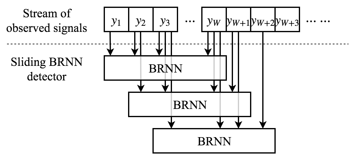
Figure 2: The sliding BRNN detector.

The detection scheme for recovering the symbols of a single UT is illustrated in Fig. 2. When the first $W$ symbols arrive at the BS, the BRNN takes the $N_{r}$ length-$W$ sequences from all receive antennas and produces a soft prediction on the symbols $(x_{1}\ldots x_{W})$ sent by the UT. When the next symbol arrives, the BRNN slides one symbol ahead, and returns the soft prediction on $(x_{2},\ldots,x_{W+1})$. The procedure is repeated until the entire signal is received. Let $\mathcal{J}_{k}=\{j|k\in[j,j+W-1]\}$ be the set of all valid starting positions of the sliding BRNN such that the prediction range covers $x_{k}$. Let $\bm{p}_{k}^{(j)}$ be the estimated probability mass function (PMF) for $x_{k}$ when the starting position of the BRNN is $j$. Note that each $\bm{p}_{k}^{(j)}$ is an $M\times 1$ vector. These initial PMFs are used to obtain the final PMF of $x_{k}$, which is estimated by averaging over $\mathcal{J}_{k}$, i.e.,

$$\bm{p}_{k}=\frac{1}{|\mathcal{J}_{k}|}\sum_{j\in\mathcal{J}_{k}}\bm{p}_{k}^{(j)}.$$ (3)

Fig. 3 shows the architecture of each BRNN adopted in this work. In particular, long short-term memory (LSTM) units with normalized outputs are used as the basic units in the BRNNs. The input $\bm{y}^{(i)}=(y_{1}^{(i)},y_{2}^{(i)},\ldots,y_{N_{r}}^{(i)})$ to each LSTM in the first layer is a $N_{r}\times 1$ vector containing the received signal at time step $i$ at all receive antennas. Then, three layers of the bidirectional LSTMs are stacked. The design of the output layer depends on the modulation scheme. When a modulation scheme with $M>2$ symbols is used by the UTs, the output layer has output size $M$ with softmax activation to estimate the PMF of the symbols. When a binary constellation, i.e., BPSK, is adopted, we simplify the output layer by using the sigmoid activation function with a scalar output, which represents the estimate of the probability that the symbol is the BSPK symbol $+1$.

Figure 3: Architecture of each BRNN.

Note that in this work, we do not include channel coding schemes that help recover the original message. The focus of this considered receiver architecture is the reliable detection of the received symbols over mmWave channels. Since the detector estimates the PMF of the symbol sequence, it is straightforward to add channel coding at the transmitter and then feed the estimated PMF to the associated soft channel decoding algorithms in the receiver.

III-B Discussion

The proposed sliding BRNN detector has several main advantages over model-based detectors for mmWave systems. First, being a data-driven detector, it requires no prior CSI at the BS, thus avoiding the difficult task of accurately estimating the exact mmWave CIR. Since the detector learns the channel conditions from the training data, there is no need to do channel estimation separately. As we show in the numerical results in Section IV, the sliding BRNN detector is quite robust to inaccurate training. In particular, it is demonstrated that a sliding BRNN detector trained using samples acquired from a set of channel realizations generated according to (2) generalizes well to a different mmWave channel realization.

Furthermore, the sliding detector structure with a moderate window length also allows for near real-time detection. In particular, the proposed detector is capable of recovering the symbol transmitted at time index $i$ once the channel output ${\bm{y}}[i+W-1]$ is received, i.e., a decoding delay of merely $W-1$ samples. To see this, we note that after receiving $W-1$ consecutive channel outputs, the detector starts to provide the PMF estimations up to the current symbol as soon as the $W$th related channel output is obtained. This allows the detector to recover the symbols without having to wait for the entire block of channel outputs to be received.

TABLE I: Running time comparison.

$N_{r}$	Sliding BRNN	Viterbi
4	0.244 s	12.461 s
128	0.264 s	52.681 s

Finally, a notable advantage of the sliding BRNN architecture compared to model-based approaches stems from the fact that, once trained, the decoding can be carried out significantly faster than iterative model-based approaches, and that this delay hardly increases as the number of antennas $N_{r}$ grows. This gain is illustrated Table I, which shows the average running time of detecting one 200-bit message using the sliding BRNN detector and the Viterbi detector measured on an AMD Phenom(tm) II X6 1045T 2.70 GHz Processor. This makes the sliding BRNN a promising decoding approach for mmWave receivers, which typically utilize massive MIMO arrays.

IV Numerical Study

In this section, we numerically evaluate the performance of our DNN-based symbol detector in terms of the detection accuracy and the convergence speed in training. The main characteristics of the simulated environment in this section are listed in Table II. The parameters $C$, $M_{c}$, $\{a_{m,c,n}\}$, $\{\phi_{m,c,n}\}$, $\tau_{m,c,n}$ in (2) are generated according to the model suggested in [15] under the parameter settings of Table II. For the sliding BRNN detector, the hidden size of each LSTM unit is 20, and the window length $W$ is set to 30. For the Viterbi detector, we use beam-search [17] with $300$ survivor paths.

TABLE II: Key parameters in simulations.

Parameter	Value
Carrier Frequency	28 GHz
Bandwidth	800 MHz
Cell Type	urban microcell
Antenna array	uniform linear array
Antenna spacing	0.5 wavelength
Transmit power	11 dBm
Tx-Rx Separation distance	60 m
Tx-Rx Antenna Gains	24.5 dBi

IV-A Error Rate Comparison

In this subsection, the performance of the sliding BRNN detector is compared with that of the Viterbi algorithm with either perfect or imperfect CSI in terms of symbol error rate (SER). In the simulations, BPSK modulation is used. The number of receive antennas is fixed to $N_{r}=4$. For each SNR value, the SER is averaged over 5 different independently generated mmWave channel realizations, and $2\times 10^{5}$ symbols, divided into blocks of $200$ symbols, are detected for each channel realization.

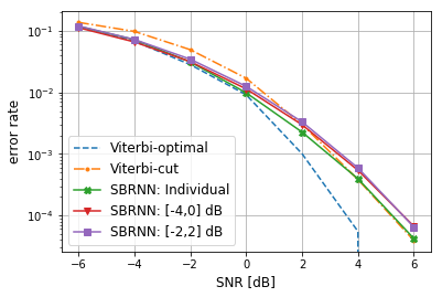
Figure 4: Comparison of SER between the sliding BRNN detector and Viterbi with perfect CSI. The sliding BRNN detector is trained with or without SNR uncertainty.

We first evaluate the SER performance of the sliding BRNN detector compared to the Viterbi detector with perfect CSI. The resulting SER values versus SNR are depicted in Fig. 4. The dashed curve in Fig. 4 is the error rate of the optimal Viterbi detector in which the detector has perfect CSI and waits to receive the entire block with the tail before detecting the symbols. This receiver implements maximum-likelihood detection for the mmWave channel. Since the sliding BRNN detector gives the detection results as soon as it receives the last symbol in the message, we also evaluate the performance of the Viterbi detector that only considers a finite window of the received signal, whose window size equals the message length. The performance of the Viterbi detector in this case is shown by the dot dashed curve with the legend “Viterbi-cut”. The solid curve with cross markers in Fig. 4 shows the error rate of the sliding BRNN detector that is trained and evaluated at the same SNR level under the same channel realization. The training set for each SNR contains 4,000 training samples, and each training sample is a tuple of a 200-symbol transmitted block $\{x[i]\}$ and the corresponding channel outputs $\{{\bm{y}}[i]\}$. It is clear that the performance of the sliding BRNN detector is close to that of the optimal Viterbi detector when the SNR is low. Note that the sliding BRNN detector only takes the received signal in a limited window for prediction, while the optimal Viterbi detector utilizes the entire received signal. When taking in the same amount of signal, the sliding BRNN detector outperforms the Viterbi-cut detector over a large range of SNR levels. This demonstrates the ability of the data-driven sliding BRNN receiver to reliably detect the transmitted symbols without requiring prior knowledge of the CSI.

To represent practical setups in which the exact value of the SNR is not known during training, we also depict in Fig. 4 the SER performance of the sliding BRNN receiver when trained using training samples corresponding to several noise levels. The legends of the curves in Fig. 4 show the range of SNR in the training signal streams. In particular, to generate the training set, we randomly pick an SNR value uniformly from the given range as the SNR for each block. After training, we use the same sliding BRNN to detect signal streams under different SNR levels. As shown in Fig. 4, the performance of the sliding BRNN decoders remain within a small gap from the Viterbi detector. It is also interesting that the sliding BRNNs trained across different SNR ranges yield similar performance. Evidently, the trained sliding BRNN generalizes well to a wide range of SNRs. These observations indicate that it suffices to train a sliding BRNN under a single SNR and use it regardless of the change to the SNR, resulting in a robust symbol detection scheme in time-varying SNR environments.

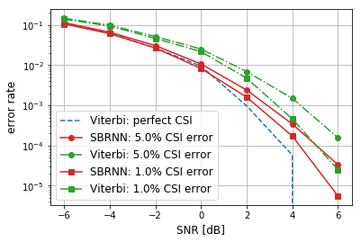
Figure 5: Comparison of SER between sliding BRNN detector and Viterbi with imperfect CSI.

Next, we numerically evaluate the generalization capability of the sliding BRNN under CSI uncertainty. In particular, we consider the case where the CSI estimate is imprecise or the channel varies slightly over time. With this aim, we evaluate the SER of the sliding BRNN detector on a mmWave channel realization whose CIR varies by $2.5\%$ or $1.0\%$ compared to the CIR used during training. Specifically, the sliding BRNN is trained under one particular channel realization and a 0 dB SNR. Then, in evaluation, we randomly distort the amplitude at each tap $\{a_{m,c,n}\}$ by $2.5\%$ or $1.0\%$ on average for each message block compared to the channel used during training. For comparison, we use the Viterbi detector with the same level of CSI error. The results of this simulation are depicted in Fig. 5, where it is observed that the sliding BRNN detector consistently outperforms the Viterbi detector with imperfect instantaneous CSI, and that the performance of the sliding BRNN remains close to the optimal Viterbi detector with perfect CSI. The result shows that the sliding BRNN detector is able to generalize well to not only the various noise levels, but also to different channel realizations.

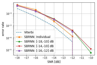
Figure 6: SER of sliding BRNN detector for SIMO with 128 receive antennas.

The numerical evaluations presented in Figs. 4-5 focused on a BS with only $4$ receive antennas. In order to demonstrate that the gains of the sliding BRNN receiver are also maintained for large antenna arrays, which are commonly utilized in mmWave communications, we depict in Fig. 6 the SER curves of the sliding BRNN detector when the number of receive antennas is $N_{r}=128$. While we do not increase the size of the neural network or the window length, the performance of the sliding BRNN detector is still close to the Viterbi detector, while the running time is significantly reduced, as discussed in Subsection III-B. Similarly to the results with fewer receive antennas presented in Fig. 4, a single sliding BRNN detector trained under a wide range of SNRs generalizes well to different noise levels. These results demonstrate the great potential of using a data-driven DNN-based detector for mmWave communications.

IV-B Training Size Analysis

Next, we numerically study the convergence speed in training the sliding BRNN detector.

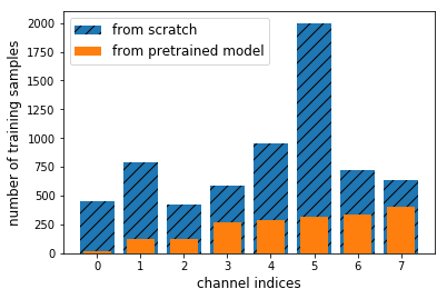
Figure 7: Comparison of convergence speed (number of training samples needed) for the sliding BRNN detector when trained from an existing model for a completely different channel realization.

To that aim, we depict in Fig. 7 the convergence time of the sliding BRNN detector. We consider two different initial values for the network weights: in the first case (filled bars in Fig. 7) the detector was already trained under some channel, and needs to be re-trained for a different channel realization. This simulates the practical scenario where the channel changes over time, and the detector needs to be adjusted to track the channel periodically. In the second case (slashed bars in Fig. 7) the weights in the sliding BRNN are randomly initialized, representing the scenario where the network is trained from scratch. In particular, $9$ different channel realizations are generated independently, indexed $0,\ldots,8$, and a sliding BRNN symbol detector trained on the last realization is utilized as the pretrained model. For each of the other $8$ channel realizations, we train the sliding BRNN detector either from scratch or from the pretrained model with the same learning rate. Fig. 7 shows the number of training samples required to achieve at least $90\%$ detection accuracy. The channels are sorted by the number of the required samples for training from a pretrained model to illustrate the distribution of the required number. Observing Fig. 7, we note that it takes many fewer samples for the sliding BRNN detector to be adapted to a new channel compared to training it from scratch. In particular, for some channel realizations, such as channels with indices 0, 1, and 2 in the figure, it takes less than $150$ samples for the detector to adapt to the new channel. This study indicates that a previously trained sliding BRNN architecture can be adjusted to time-varying channel conditions with minimal overhead for re-training the network.

V Conclusions

This paper studied a DNN-based symbol detector for uplink mmWave communications, which does not require CSI and learns the decoding mapping in a data-driven fashion. Our proposed receiver was based on a sliding BRNN architecture, which is suitable for the long channel memory and large number of receive antennas commonly used in mmWave systems. Numerical evaluations demonstrated that the sliding BRNN detector is capable of achieving performance within a small gap from the optimal Viterbi detector, which requires full CSI. Moreover, the sliding BRNN detector was shown to generalize well when trained using samples taken from an inaccurate model, and in fact it outperformed the Viterbi detector with the same level of CSI uncertainty. Finally, we numerically showed that a pretrained DNN detector could be adjusted to another channel realization with minimal overhead.

References

- [1] T. Rappaport, S. Sun, R. Mayzus, H. Zhao, Y. Azar, K. Wang, G. Wong, J. Schulz, M. Samimi, and F. Gutierrez. “Millimeter Wave mobile communications for 5G cellular: it will work!”. IEEE Access, vol. 1, pp. 335–349, May 2013.
- [2] M. Akdeniz, Y. Liu, S. Sun, S. Rangan, T. Rappaport, and E. Erkip. “Millimeter wave channel modeling and cellular capacity evaluation”. IEEE J. Sel. Areas in Commun., vol. 32, no. 6, pp. 1164–1179, Jun. 2014.
- [3] T. O’Shea and J. Hoydis. “An introduction to deep learning for the physical layer”. IEEE Trans. on Cogn. Commun. Netw., vol. 3, no. 4, Dec. 2017, pp. 563–575.
- [4] Q. Mao, F. Hu and Q. Hao. “Deep learning for intelligent wireless networks: A comprehensive survey”. IEEE Commun. Surveys Tuts., vol. 20, no. 4, 2018, pp. 2595–2621.
- [5] O. Simeone. “A very brief introduction to machine learning with applications to communication systems”. IEEE Trans. on Cogn. Commun. Netw., vol. 4, no. 4, Dec. 2018, pp. 648–664.
- [6] E. Nachmani, Y. Be’ery, and D. Burshtein. “Learning to decode linear codes using deep learning”. in 54th Annual Allerton Conference on Communication, Control, and Computing, Sep. 2016, pp. 341–-346.
- [7] T. O’Shea, K. Karra, and T. C. Clancy. “Learning to communicate: Channel auto-encoders, domain specific regularizers, and attention”. in 2016 IEEE International Symposium on Signal Processing and Information Technology (ISSPIT), Dec 2016, pp. 223–-228.
- [8] N. Shlezinger, N. Farsad, Y. C. Eldar, and A. J. Goldsmith. “ViterbiNet: Symbol detection using a deep learning based Viterbi algorithm”. Submitted to SPAWC, Cannes, France, Jul. 2019.
- [9] N. Farsad and A. Goldsmith. “Neural network detection of data sequences in communication systems”. IEEE Trans. Signal Process., vol. 66, no. 21, Nov. 2018, pp. 5663–5678.
- [10] H. He , C-K. Wen , S. Jin , and G. Li. “Predicting wireless mmWave massive MIMO channel characteristics using machine learning algorithms”. IEEE Wireless Commum. Letters, vol. 7, no. 5, Oct. 2018, pp. 852–855.
- [11] H. Huang, Y. Song, J. Yang, G. Gui, and F. Adachi. “Deep-learning-based millimeter-Wave massive MIMO for hybrid precoding”. arXiv preprint, arXiv: 1901.06537, 2019
- [12] P. Zhou, X. Fang, X. Wang, Y. Long, R. He, and X. Han. “Deep learning-based beam management and interference coordination in dense mmWave networks”. IEEE Trans. on Vehicular Tech., vol. 68, no. 1, Jan. 2019, pp. 592-603.
- [13] T. L. Marzetta. “Noncooperative cellular wireless with unlimited numbers of base station antenna”. IEEE Trans. Wireless Commun., vol. 9, no. 11, Nov. 2010, pp. 3950–3600.
- [14] S. Verdu. Multiuser Detection. Cambridge Press, 1998.
- [15] M. Samimi, and T. Rappaport. “3-D millimeter-wave statistical channel model for 5G wireless system design”. IEEE Trans. Microwave Theory and Techniques, vol. 64, no. 7, Jul. 2016, pp. 2207–2225.
- [16] 3GPP TR 38.901. Study on channel model for frequencies from 0.5 to 100 GHz simulations, 2018.
- [17] X. Lingyun and D. Limin. “Efficient Viterbi beam search algorithm using dynamic pruning”. Proc. ICSP, Beijing, China, Aug. 2004.