Asymmetric behavior of surface waves
induced by an underlying interfacial wave

Abstract

We develop a weakly nonlinear model to study the spatiotemporal manifestation and the dynamical behavior of surface waves in the presence of an underlying interfacial solitary wave in a two-layer fluid system. We show that interfacial solitary-wave solutions of this model can capture the ubiquitous broadening of large-amplitude internal waves in the ocean. In addition, the model is capable of capturing three asymmetric behaviors of surface waves: (i) Surface waves become short in wavelength at the leading edge and long at the trailing edge of an underlying interfacial solitary wave. (ii) Surface waves propagate towards the trailing edge with a relatively small group velocity, and towards the leading edge with a relatively large group velocity. (iii) Surface waves become high in amplitude at the leading edge and low at the trailing edge. These asymmetric behaviors can be well quantified in the theoretical framework of ray-based theories. Our model is relatively easily tractable both theoretically and numerically, thus facilitating the understanding of the surface signature of the observed internal waves.

Keywords. interfacial waves, surface waves, ray-based theory

Mathematics Subject Classification. 76B55; 76B07; 35L05; 65M22

1 Introduction

Internal waves with large amplitudes and long wavelengths are widely observed in coastal ocean regions, and are believed to be important for transferring momentum, heat, and energy in the ocean [30, 28]. Because of their strong turbulent mixing and breaking, they can influence many ocean processes, such as nutrient supply, sediment and pollutant transport, acoustic transmission, and interaction with man-made structures [20, 3]. Generated by tidal flow, internal waves usually can propagate thousands of kilometers from their source before dissipation, sloping, and breaking extinguish them [28, 5]. In recent decades, observation data for internal waves and their corresponding surface signature have been recorded using in situ measurements and Synthetic Aperture Radar (SAR) in many coastal seas worldwide [38, 20, 3].

Many previous studies have investigated the interaction between interfacial waves (IWs) and surface waves (SWs) in two-layer fluid systems. These works can be broadly subdivided into two classes. The first class focuses on the issue of addressing the direct numerical simulation of the Laplace equations for velocity potentials with the appropriate boundary conditions in a two-layer fluid system [2, 43]. The system can be formulated as a Hamiltonian system for a set of canonical variables [4, 2]. To evaluate the time derivatives of these canonical variables, the high-order spectral (HOS) method [2] is employed to solve the boundary value problems of Laplace equations. By applying the HOS method, it was found that energy can be transferred from SWs to IWs in the two-layer fluid system [43]. However, the direct numerical simulations are typically expensive, and it is also challenging to extract the mechanism underlying their results.

The second class focuses on the reduced models in the two-layer fluid system. To overcome the difficulty stemming from expensive computations, a common approach is to study a reduced model of the two-layer Euler system via multi-scale analysis [32, 27, 23, 19, 39, 6, 8, 29, 17]. These reduced models describing two-layer fluids mostly focus on three aspects:

[a] Traveling wave solutions: Traveling-wave solutions exhibiting oscillations are found in the reduced models. For example, generalized solitary waves with non-decaying oscillations along their tails in addition to the solitary pulse were found in a long-wave model [18, 39, 22]. Besides the generalized solitary waves, multi-humped solitary waves with a finite number of oscillations riding on the solitary pulse were found in a fully-nonlinear long-wave model [8].

[b] Ray-based theories: Many ray-based studies take a statistical viewpoint of SWs modulated by a near-surface current induced by IWs [24, 37, 9, 6, 5]. These studies invoke phase-averaged models based on a wave-balance equation and ray-based theory [9, 6], which can be applied to the remote-sensing observations of IWs via their surface manifestations.

[c] Resonant excitations: When two different modes coexist in a fluid system, a resonant interaction becomes possible between the modes to aid in transferring energy in the ocean [41]. Class 3 triad resonance is regarded as being responsible for the surface signature of the underlying IWs [41, 38, 27, 23, 16, 1]. Based on a class 3 triad resonance condition, many reduced models have been derived for the interfacial and surface waves[37, 32, 27, 23, 42, 36, 29, 17]. A detailed discussion of surface signature phenomena of IWs was presented in [16, 14, 15, 17] using a coupled Korteweg–de Vries (KdV) and a linear Schrödinger model. Narrow rough regions containing surface ripples were found and interpreted as a result of the energy accumulation in the localized bound states of the Schrödinger equation [17].

Different from previous works, we here develop a new reduced model to investigate the spatiotemporal manifestation of the small-amplitude SWs in the presence of an interfacial solitary wave in the two-layer setting. Based on model simulations, we demonstrate that our model is successful in characterizing many types of dynamical behavior of SWs, which can be well understood using the ray-based theories. In Sec. 2, we derive a reduced model for the two-layer fluid system. In Sec. 3, we analyze the basic properties of the model, including interfacial solitary-wave solutions and dispersion relations. In Sec. 4, we present the numerical scheme and examine its numerical convergence. In Sec. 5, we show the numerical results for the asymmetric behavior of SWs and quantify this asymmetric behavior using the ray-based theories. Conclusions and discussion are given in Sec. 6, and some mathematical details are presented in the Appendix.

2 The two-layer weakly nonlinear (TWN) model

We first introduce Euler equations for two immiscible layers of potential fluids with unequal densities. The two layers of fluids are assumed to be inviscid, irrotational, and incompressible. The unequal densities for the upper layer and for the lower layer are denoted by $\rho_{1}$ and $\rho_{2}$, respectively. Here, $\rho_{2}>\rho_{1}$ is assumed for the stable case. The horizontal and vertical coordinates are $x$ and $z$, respectively. We focus on the evolution of large-amplitude interfacial waves $\xi_{2}$ between the two fluid layers, and their coupling with the the overlaying free surface, $\xi_{1}$ [see Fig. 1]. The velocity potential $\phi_{i}$ ($i=1$ for the upper layer and $i=2$ for the lower layer) satisfies Laplace’s equation,

$$\phi_{ixx}+\phi_{izz}=0.$$ (2.1)

The kinematic equations for the continuity of the normal velocity at the surface $h_{1}+\xi_{1}$, the interface $\xi_{2}$, and the flat topography $-h_{2}$ are given in the form

$$\xi_{1t}+\phi_{1x}\xi_{1x}=\phi_{1z},\text{ \ \ at }z=h_{1}+\xi_{1},$$ (2.2)

$$\xi_{2t}+\phi_{1x}\xi_{2x}=\phi_{1z},\text{ \ \ at }z=\xi_{2},$$ (2.3)

$$\xi_{2t}+\phi_{2x}\xi_{2x}=\phi_{2z},\text{ \ \ at }z=\xi_{2},$$ (2.4)

$$\phi_{2z}=0,\text{ \ \ at }z=-h_{2},$$ (2.5)

where $h_{1}$ and $h_{2}$ are the undisturbed thicknesses of the upper and lower layers, respectively. The dynamical equations for the continuity of pressure at the surface and the interface are the Bernoulli equations,

$$\phi_{1t}+\frac{1}{2}\left(\phi_{1x}^{2}+\phi_{1z}^{2}\right)+g\xi_{1}=0,\text{ \ \ at }z=h_{1}+\xi_{1},$$ (2.6)

$$\rho_{1}\left(\phi_{1t}+\frac{1}{2}\left(\phi_{1x}^{2}+\phi_{1z}^{2}\right)+g\xi_{2}\right) =\rho_{2}\left(\phi_{2t}+\frac{1}{2}\left(\phi_{2x}^{2}+\phi_{2z}^{2}\right)+g\xi_{2}\right),$$ (2.7)

$$\text{at \ \ }z =\xi_{2}.$$

where $g$ is the gravitational acceleration.

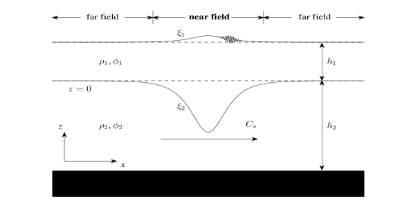
Figure 1: Sketch of the two-layer fluid system [see text].

For the small-amplitude approximation, we assume that the characteristic amplitude, $a$, of the IWs and SWs is much smaller than the thickness of the two fluid layers,

$$a/h_{1}=\alpha\ll 1,\ \ \ h_{2}/h_{1}=O(1).$$ (2.8)

For the long-wave approximation, we assume that the thickness of each fluid layer is much smaller than the characteristic wavelength, $L$, of the IWs and SWs,

$$h_{1}^{2}/L^{2}=\beta\ll 1,\ \ \ h_{2}/h_{1}=O(1).$$ (2.9)

The two small parameters, $\alpha$ and $\beta$, control the nonlinear and dispersive effects, respectively. Based on the scaling (2.8)-(2.9), we may nondimensionalize all the physical variables by taking the original variables to be

$$x=Lx^{\ast},\text{ \ \ }z=h_{1}z^{\ast},\text{ \ \ }t=(L/U_{0})t^{\ast},$$

$$\left(\phi_{1},\phi_{2}\right)=\left(aLU_{0}/h_{1}\right)\left(\phi_{1}^{\ast},\phi_{2}^{\ast}\right),\text{ \ \ }(\xi_{1},\xi_{2})=a(\xi_{1}^{\ast},\xi_{2}^{\ast}),$$ (2.10)

where $U_{0}=\sqrt{gh_{1}}$ is the characteristic speed of the gravity waves. Here, all the variables with asterisks are assumed to be $O(1)$ in $\alpha$ and $\beta$. In the dimensionless, starred variables, Laplace’s equation (2.1) is formulated as

$$\beta\phi_{ix^{\ast}x^{\ast}}^{\ast}+\phi_{iz^{\ast}z^{\ast}}^{\ast}=0,\ \ \ {\rm for\ }i=1,2.$$ (2.11)

We first focus on the upper fluid layer. The analogous derivation for the lower fluid layer follows a similar procedure. We seek an asymptotic expansion of $\phi_{1}^{\ast}$ in powers of $\beta$,

$$\phi_{1}^{\ast}=\phi_{1}^{\ast(0)}+\beta\phi_{1}^{\ast(1)}+O(\beta^{2}),$$ (2.12)

which we use in the asymptotic analysis of the nondimensionalized problem of equations (2.1)-(2.7) for small values of the parameter $\beta$. From the leading $O(1)$ term in Eqs. (2.1) and (2.2), $\phi_{1}^{\ast(0)}$ is found to be independent of the height $z$,

$$\phi_{1}^{\ast(0)}=\phi_{1}^{\ast(0)}(x^{\ast},t^{\ast}).$$ (2.13)

The $O(\beta)$ terms in Eqs. (2.1) and (2.2) yield the equations

$$\phi_{1x^{\ast}x^{\ast}}^{\ast(0)}+\phi_{1z^{\ast}z^{\ast}}^{\ast(1)}=0,\text{ \ \ }\alpha\xi_{2}^{\ast}<z^{\ast}<h_{1}^{\ast}+\alpha\xi_{1}^{\ast},\text{ with }h_{1}^{\ast}=1,$$

$$\phi_{1z^{\ast}}^{\ast(1)}=\xi_{1t^{\ast}}^{\ast}+\alpha\phi_{1x^{\ast}}^{\ast(0)}\xi_{1x^{\ast}}^{\ast},\text{ \ \ at }z^{\ast}=h_{1}^{\ast}+\alpha\xi_{1}^{\ast}.$$ (2.14)

The expression for $\phi_{1}^{\ast(1)}$ is obtained as

$$\phi_{1}^{\ast(1)}=D_{1}\xi_{1}^{\ast}Z_{1}-\frac{1}{2}\phi_{1x^{\ast}x^{\ast}}^{\ast(0)}Z_{1}^{2},$$ (2.15)

where $Z_{1}=z^{\ast}-h_{1}^{\ast}-\alpha\xi_{1}^{\ast}$ and $D_{1}\xi_{1}^{\ast}\equiv\xi_{1t^{\ast}}^{\ast}+\alpha\phi_{1x^{\ast}}^{\ast(0)}\xi_{1x^{\ast}}^{\ast}$. Combining expressions (2.13) and (2.15), to the first power of $\beta$, we can obtain the solution $\phi_{1}^{\ast}$ as

$$\phi_{1}^{\ast}=\phi_{1}^{\ast(0)}+\beta\left(D_{1}\xi_{1}^{\ast}Z_{1}-\frac{1}{2}\phi_{1x^{\ast}x^{\ast}}^{\ast(0)}Z_{1}^{2}\right)+O(\beta^{2}).$$ (2.16)

By integrating Eq. (2.1) once from $\alpha\xi_{2}^{\ast}$ to $h_{1}^{\ast}+\alpha\xi_{1}^{\ast}$ with respect to $z^{\ast}$, imposing the boundary conditions (2.2) and (2.3), and substituting the expression (2.16) into equation (2.1), we obtain the kinematic equation for the upper fluid layer,

$$\eta_{1t^{\ast}}^{\ast}+\left(\eta_{1}^{\ast}\widetilde{u}_{1}^{\ast}\right)_{x^{\ast}}-\frac{1}{6}\beta\left(h_{1}^{\ast}\right)^{3}\widetilde{u}_{1x^{\ast}x^{\ast}x^{\ast}}^{\ast}-\frac{1}{2}\beta\left(h_{1}^{\ast}\right)^{2}\xi_{1t^{\ast}x^{\ast}x^{\ast}}+O(\alpha\beta,\beta^{2})=0,$$ (2.17)

where

$$\eta_{1}^{\ast}=h_{1}^{\ast}+\alpha\xi_{1}^{\ast}-\alpha\xi_{2}^{\ast},\text{ \ \ }\widetilde{u}_{1}^{\ast}=\phi_{1x^{\ast}}^{\ast(0)}.$$

Upon substitution of the velocity potential $\phi_{1}^{\ast}$ (2.16) into the dynamical boundary condition (2.6), we obtain the dynamical equation governing the motion of the upper fluid layer,

$$\widetilde{u}_{1t^{\ast}}^{\ast}+\alpha\widetilde{u}_{1}^{\ast}\widetilde{u}_{1x^{\ast}}^{\ast}+g\xi_{1x^{\ast}}^{\ast}+O(\alpha\beta,\beta^{2})=0,$$ (2.18)

where the equation has been differentiated with respect to $x^{\ast}$ once, the terms in the first power of $\beta$ are retained [the $O(\beta)$ terms happen to vanish in Eq. (2.18)], and terms of $O(\alpha\beta,\beta^{2})$ are dropped. From the velocity potential $\phi_{1}^{\ast}$, (2.16), we obtain the horizontal velocity $\phi_{1x^{\ast}}^{\ast}$ as

$$\phi_{1x^{\ast}}^{\ast}=\widetilde{u}_{1}^{\ast}+\beta\xi_{1t^{\ast}x^{\ast}}^{\ast}Z_{1}-\frac{1}{2}\beta\widetilde{u}_{1x^{\ast}x^{\ast}}^{\ast}Z_{1}^{2}+O(\alpha\beta,\beta^{2}).$$ (2.19)

By averaging (2.19) over the depth, we obtain the layer-mean horizontal velocity for the upper fluid layer,

$$\overline{u}_{1}^{\ast}=\widetilde{u}_{1}^{\ast}-\frac{1}{2}\beta h_{1}^{\ast}\xi_{1t^{\ast}x^{\ast}}^{\ast}-\frac{1}{6}\beta\left(h_{1}^{\ast}\right)^{2}\widetilde{u}_{1x^{\ast}x^{\ast}}^{\ast}+O(\alpha\beta,\beta^{2});$$

the corresponding inverse is

$$\widetilde{u}_{1}^{\ast}=\overline{u}_{1}^{\ast}+\frac{1}{2}\beta h_{1}^{\ast}\xi_{1t^{\ast}x^{\ast}}^{\ast}+\frac{1}{6}\beta\left(h_{1}^{\ast}\right)^{2}\overline{u}_{1x^{\ast}x^{\ast}}^{\ast}+O(\alpha\beta,\beta^{2}),$$ (2.20)

where the layer-mean horizontal velocity is defined as

$$\overline{u}_{1}^{\ast}(x^{\ast},t^{\ast})=\displaystyle\dfrac{1}{\eta_{1}^{\ast}}\int_{\alpha\xi_{2}^{\ast}}^{h_{1}^{\ast}+\alpha\xi_{1}^{\ast}}\phi_{1x^{\ast}}^{\ast}(x^{\ast},z^{\ast},t^{\ast})dz^{\ast}.$$

After substituting Eq. (2.20) for the horizontal velocity $\widetilde{u}_{1}^{\ast}$, equations (2.17) and (2.18) provide Boussinesq-type equations governing the motion of the fluid in the upper layer.

Repeating a similar procedure, we can obtain the governing equations for the lower fluid layer. The final set of equations for the variables $(\xi_{1},\xi_{2},\overline{u}_{1},\overline{u}_{2})$, in the dimensional form, is

$$\eta_{1t}+(\eta_{1}\overline{u}_{1})_{x}=0,\text{ \ \ }\eta_{1}=h_{1}+\xi_{1}-\xi_{2},$$ (2.21)

$$\eta_{2t}+(\eta_{2}\overline{u}_{2})_{x}=0,\text{ \ \ }\eta_{2}=h_{2}+\xi_{2},$$ (2.22)

$$\overline{u}_{1t}+\overline{u}_{1}\overline{u}_{1x}+g\xi_{1x}-\frac{1}{3}h_{1}^{2}\overline{u}_{1xxt}+\frac{1}{2}h_{1}\xi_{2ttx}=0,$$ (2.23)

$$\overline{u}_{2t}+\overline{u}_{2}\overline{u}_{2x}+g\xi_{2x}+\rho_{r}g\eta_{1x}$$ (2.24)

$$-\frac{1}{2}\rho_{r}h_{1}^{2}\overline{u}_{1xxt}+\rho_{r}h_{1}\xi_{2ttx}-\frac{1}{3}h_{2}^{2}\overline{u}_{2xxt}=0,$$

where $\rho_{r}$ is the density ratio $\rho_{1}/\rho_{2}$, and

$$\overline{u}_{1}(x,t)=\dfrac{1}{\eta_{1}}\int_{\xi_{2}}^{h_{1}+\xi_{1}}\phi_{1x}(x,z,t)dz,\ \ \ \overline{u}_{2}(x,t)=\dfrac{1}{\eta_{2}}\int_{-h_{2}}^{\xi_{2}}\phi_{2x}(x,z,t)dz,$$

are the layer-mean horizontal velocities. We refer to the model (2.21)-(2.24) as the two-layer weakly-nonlinear model or TWN model. The TWN model can also be obtained via a direct reduction from a fully nonlinear model (to which we refer as MCC model) given in [12, 8, 7]. For the numerical examples throughout the paper, all the variables and parameters are dimensionless and the parameters are fixed to be $(h_{1},h_{2},g,\rho_{1},\rho_{2})=(1,3,1,1,1.003)$. In particular, in our simulations, the characteristic length in both height and wavelength is $h_{1}$, the characteristic speed is $\sqrt{gh_{1}}$, and the characteristic time is $\sqrt{h_{1}/g}$ [see similar dimensionless forms used in numerical simulations in [13, 11]]. Note that, without loss of generality, our conclusions concerning broadening of IWs in Sec. 3.1 and asymmetric behavior of SWs in Sec. 5 also hold true for other parameter regimes of $(h_{1},h_{2},g,\rho_{1},\rho_{2})$.

3 Basic properties of the TWN model

In this section, we study some basic properties of the TWN model, including interfacial solitary wave solutions and dispersion relations.

3.1 Interfacial solitary-wave solution

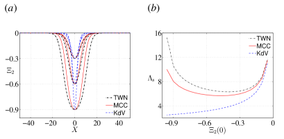
Figure 2: (Color online) Comparison of interfacial solitary-wave solutions among our TWN model [Eqs. (3.27)-(3.28)], the MCC model [13], and the KdV model [13]. (a) Profiles of interfacial solitary-wave solutions with the same amplitude. (b) Effective width $\Lambda_{s}$ versus wave amplitude $\Xi_{2}(0)$. As the amplitude increases, the solitary-wave solutions broaden and eventually develop a flat crest when the amplitude increases to approximately $(h_{1}-h_{2})/2$. The TWN model and MCC model can capture the broadening of IWs whereas the KdV model cannot.

To study the behavior of the overlaying SWs when an interfacial solitary wave moves beneath the surface, we first seek interfacial solitary-wave solutions of the TWN model (2.21)-(2.24). Then, we use these solitary-wave solutions as initial conditions for wave profiles and layer-mean velocities for the subsequent numerical simulations in Sec. 5. To look for the right-moving traveling waves that propagate with the nonlinear phase velocity $C_{s}$, we assume the following ansatz for the surface elevation, internal elevation, upper-layer velocity, and lower-layer velocity, $(\xi_{i},\overline{u}_{i})$ [$i=1,2$], in the system (2.21)-(2.24):

$$\xi_{i}\left(x,t\right)=\Xi_{i}\left(X\right),\text{ \ \ }\overline{u}_{i}\left(x,t\right)=\overline{U}_{i}\left(X\right),\text{ \ \ }X=x-C_{s}t.$$ (3.25)

Substituting this ansatz into Eqs. (2.21)-(2.22) and integrating once with respect to $X$ yields

$$\overline{U}_{i}=\frac{C_{s}\left(H_{i}-h_{i}\right)}{H_{i}},\text{ with }H_{1}=h_{1}+\Xi_{1}-\Xi_{2}\text{ and }H_{2}=h_{2}+\Xi_{2},$$ (3.26)

where we have assumed that $H_{i}\rightarrow h_{i}$ as $X\rightarrow\pm\infty$, and $h_{1}$ ($h_{2}$) is the undisturbed thickness of the upper (lower) fluid layer, respectively. Substituting the horizontal velocity (3.26) for $\overline{U}_{i}$ into Eqs. (2.23)-(2.24) and integrating once with respect to $X$ leads to the equations

$$-\frac{1}{3}C_{s}^{2}h_{1}^{3}\frac{H_{1XX}}{H_{1}^{2}}-\frac{1}{2}C_{s}^{2}h_{1}H_{2XX}$$ (3.27)

$$=\frac{C_{s}^{2}h_{1}^{2}}{2}\left(\frac{1}{H_{1}^{2}}-\frac{1}{h_{1}^{2}}\right) +g\left(H_{1}+H_{2}-h_{1}-h_{2}\right)-\frac{2}{3}C_{s}^{2}h_{1}^{3}\frac{H_{1X}^{2}}{H_{1}^{3}},$$

$$-\frac{1}{2}\rho_{r}C_{s}^{2}h_{1}^{3}\frac{H_{1XX}}{H_{1}^{2}}-\rho_{r}C_{s}^{2}h_{1}H_{2XX}-\frac{1}{3}C_{s}^{2}h_{2}^{3}\frac{H_{2XX}}{H_{2}^{2}}$$ (3.28)

$$=\frac{C_{s}^{2}h_{2}^{2}}{2}\left(\frac{1}{H_{2}^{2}}-\frac{1}{h_{2}^{2}}\right)+g\left(H_{2}-h_{2}\right)+\rho_{r}g\left(H_{1}-h_{1}\right) -\rho_{r}C_{s}^{2}h_{1}^{3}\frac{H_{1X}^{2}}{H_{1}^{3}}-\frac{2}{3}C_{s}^{2}h_{2}^{3}\frac{H_{2X}^{2}}{H_{2}^{3}},$$

where we have assumed that $H_{iX}$, $H_{iXX}\rightarrow 0$ as $X\rightarrow\pm\infty$ for $i=1,2$. Since explicit solutions to Eqs. (3.27)-(3.28) are difficult to establish, we numerically compute their solitary-wave solutions by applying the method in [26].

In Fig. 2(a), we show the numerical solutions of the TWN model for IWs with different amplitudes. For comparison, we also show the corresponding MCC and KdV solutions with the same amplitudes [13]. From Fig. 2(a), we can see that the TWN model and the MCC model can capture the broadening of internal waves that is often observed in the ocean. For instance, a single large internal wave in $340$ meters of water was observed in the northeastern South China Sea by [21]. The typical wavelength of the observed internal wave is longer than the KdV solution of the same amplitude that is used to fit this internal wave. It is worthwhile to mention that the broadening of interfacial solitary wave solutions can also be captured by other models [15, 25], not only by the MCC-type models.

To quantify this broadening, we introduce a measure of the effective width, $\Lambda_{s}$, for the interfacial solitary-wave solution [34], defined as

$$\Lambda_{s}=\left|\frac{1}{\Xi_{2}(0)}\int_{0}^{\infty}\Xi_{2}(X)dX\right|.$$ (3.29)

Meanwhile, the effective width of MCC and KdV solutions are provided in the reference [13]. Figure 2(b) displays the comparison of effective width among the TWN solutions, MCC solutions, and KdV solutions. When the amplitude of waves is small, there is good agreement of the effective widths among all solutions. However, when the amplitude of the waves becomes large, discrepancy grows rapidly among these three solutions. When the amplitude increases to the limiting value, approximately $(h_{1}-h_{2})/2$, the TWN and MCC solutions become much broader than the KdV solutions. The maximum amplitude of our TWN model is approximately $(h_{1}-h_{2})/2$. Beyond the maximum amplitude, no solitary waves can exist for IWs.

3.2 Dispersion relations

We now investigate the dispersion relation of the TWN model (2.21)-(2.24) using linear analysis. By substituting the monochromatic solutions $(\xi_{i},\overline{u}_{i})\sim\exp[{\text{i}}(kx-\mu_{k}t)]$ into the system (2.21)-(2.24), the pure linear dispersion relation in the absence of shear between the frequency $\mu_{k}$ and the wavenumber $k$ can be obtained as

$$\left(1+\rho_{r}k^{2}h_{1}h_{2}+\frac{1}{3}k^{2}h_{1}^{2}+\frac{1}{3}k^{2}h_{2}^{2}+\frac{1}{9}k^{4}h_{1}^{2}h_{2}^{2}+\frac{1}{12}\rho_{r}k^{4}h_{1}^{3}h_{2}\right)\mu_{k}^{4}$$ (3.30)

$$-\left(gh_{1}+gh_{2}+\frac{1}{3}gk^{2}h_{1}h_{2}^{2}+\frac{1}{3}gk^{2}h_{1}^{2}h_{2}\right)k^{2}\mu_{k}^{2}+\left(1-\rho_{r}\right)g^{2}k^{4}h_{1}h_{2}=0.$$

Here, the shear is the interface and velocity jump induced by an interfacial solitary wave. The same dispersion relation can be found in [8].

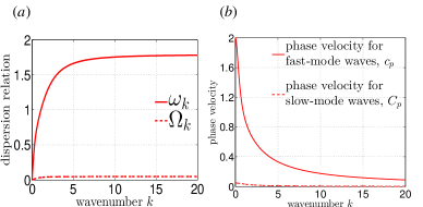
Figure 3: (Color online) (a) Pure linear dispersion relations $\Omega_{k}$ for slow-mode waves [Eq. (3.31)] and $\omega_{k}$ for fast-mode waves [Eq. (3.32)]. (b) Phase velocities $C_{p}$ for slow-mode waves and $c_{p}$ for fast-mode waves.

Equation (3.30) has $4$ real roots in the oceanic regime (the density ratio $\rho_{r}$ is close to $1$). At the leading order in $1-\rho_{r}$, the dispersion relations of the two-mode waves, denoted by $\Omega_{k}$ and $\omega_{k}$ [see Fig. 3], can be approximated as

$$\Omega_{k}^{2}=\frac{\left(1-\rho_{r}\right)g^{2}h_{1}h_{2}k^{2}}{gh_{1}+gh_{2}+\frac{1}{3}gk^{2}h_{1}h_{2}^{2}+\frac{1}{3}gk^{2}h_{1}^{2}h_{2}},$$ (3.31)

and

$$\omega_{k}^{2}=\frac{\left(gh_{1}+gh_{2}+\frac{1}{3}gk^{2}h_{1}h_{2}^{2}+\frac{1}{3}gk^{2}h_{1}^{2}h_{2}\right)k^{2}}{1+\rho_{r}k^{2}h_{1}h_{2}+\frac{1}{3}k^{2}h_{1}^{2}+\frac{1}{3}k^{2}h_{2}^{2}+\frac{1}{9}k^{4}h_{1}^{2}h_{2}^{2}+\frac{1}{12}\rho_{r}k^{4}h_{1}^{3}h_{2}}.$$ (3.32)

In the following, the two kinds of waves that correspond to the dispersion relations $\Omega_{k}$, (3.31), and $\omega_{k}$, (3.32), are referred to as the slow-mode waves and the fast-mode waves, respectively.

The modulated dispersion relation $\overline{\omega}_{k}$ in the presence of shear can be obtained by substituting $(\xi_{i},\overline{u}_{i})\sim(\Xi_{i},\overline{U}_{i})+\exp[{\text{i}}(kx-\overline{\omega}_{k}t)]$ into the system (2.21)-(2.24), where the shear is induced by an interfacial solitary wave $(\Xi_{i},\overline{U}_{i})$ in above Sec. 3.1. The resulting equation is

$$\left|\begin{array}[]{cccc}-\overline{\omega}_{k}+k\overline{U}_{1}&\overline{\omega}_{k}-k\overline{U}_{1}&kh_{1}+k\Xi_{1}-k\Xi_{2}&0\\ 0&-\overline{\omega}_{k}+k\overline{U}_{2}&0&kh_{2}+k\Xi_{2}\\ gk&-\frac{1}{2}kh_{1}\overline{\omega}_{k}^{2}&-\overline{\omega}_{k}-\frac{1}{3}k^{2}h_{1}^{2}\overline{\omega}_{k}+k\overline{U}_{1}&0\\ \rho_{r}gk&(1-\rho_{r})gk-\rho_{r}kh_{1}\overline{\omega}_{k}^{2}&-\frac{1}{2}\rho_{r}k^{2}h_{1}^{2}\overline{\omega}_{k}&-\overline{\omega}_{k}-\frac{1}{3}k^{2}h_{2}^{2}\overline{\omega}_{k}+k\overline{U}_{2}\end{array}\right|=0,$$ (3.33)

where $\left|\cdot\right|$ denotes the determinant of the enclosed matrix. In the following Secs. 4 and 5, we will numerically study the TWN model in the right-moving frame with the nonlinear phase velocity $C_{s}$, that is, $T=t$ and $X=x-C_{s}t$. Note that the solitary-wave solutions $(\Xi_{i},\overline{U}_{i})$ are steady in time $T$ in this moving frame. Then, the modulated dispersion relation $\overline{\nu}$, corresponding to the moving frame $T$ and $X$, is given by

$$\overline{\nu}_{k}=\overline{\omega}_{k}-C_{s}k,$$ (3.34)

where $\overline{\omega}_{k}$ is the modulated dispersion relation in Eq. (3.33) corresponding to the resting frame $t$ and $x$. Note that the dispersion relation $\overline{\nu}_{k}$ is independent of time $T$ since $(\Xi_{i},\overline{U}_{i})$ are steady in time $T$. Moreover, the wavelengths of $(\Xi_{i},\overline{U}_{i})$ are relatively long with respect to the characteristic wavelengths of fast-mode waves, so $(\Xi_{i},\overline{U}_{i})$ in the dispersion relation $\overline{\nu}_{k}$ can be locally treated as constant in $X$ space.

4 Numerical scheme

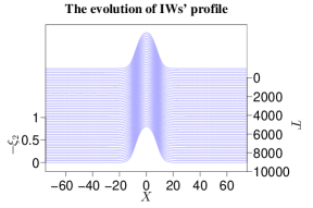
Figure 4: (Color online) Spatiotemporal evolution of the interfacial solitary-wave solution $\xi_{2}$ with the amplitude being $-0.8$ during the time period $0\leq T\leq 10000$. The maximal amplitudes of $(\xi_{1},\xi_{2},\overline{u}_{1},\overline{u}_{2})$ are $(0.001,-0.8,0.024,-0.019)$. The time step is $\Delta T=0.1$ and the spatial discretization is $\Delta X=600/2^{14}$.

For numerical computations, we cast Eqs. (2.21)-(2.24) in the conservation form in the right-moving frame with the nonlinear phase velocity (soliton speed) $C_{s}$ as follows:

$$\eta_{1T}-C_{s}\eta_{1X}+(\eta_{1}\overline{u}_{1})_{X}=0,$$ (4.35)

$$\eta_{2T}-C_{s}\eta_{2X}+(\eta_{2}\overline{u}_{2})_{X}=0,$$ (4.36)

$$M_{1T}-C_{s}M_{1X}+\left(\frac{1}{2}\overline{u}_{1}^{2}+g\xi_{1}\right)_{X}=0,$$ (4.37)

$$M_{2T}-C_{s}M_{2X}+\left(\frac{1}{2}\overline{u}_{2}^{2}+g\xi_{2}+\rho_{r}g\eta_{1}\right)_{X}=0,$$ (4.38)

where

$$M_{1}=\overline{u}_{1}-\frac{1}{3}h_{1}^{2}\overline{u}_{1XX}-\frac{1}{2}h_{1}\left(\eta_{2}\overline{u}_{2}\right)_{XX},$$ (4.39)

$$M_{2}=\overline{u}_{2}-\frac{1}{2}\rho_{r}h_{1}^{2}\overline{u}_{1XX}-\frac{1}{3}h_{2}^{2}\overline{u}_{2XX}-\rho_{r}h_{1}\left(\eta_{2}\overline{u}_{2}\right)_{XX},$$ (4.40)

and $T=t$, $X=x-C_{s}t$. The computational domain is set to be $[-M,M]$, with periodic boundary conditions. Even for an initially narrowly localized perturbation wave, radiation can be quickly emitted towards the two boundaries $x=-M$ and $x=M$. To eliminate possible reflected waves from these boundaries, two buffer zones in the regions $[-M,-M/2]$ and $[M/2,M]$ are established, and damping and diffusion terms are added to absorb the outgoing radiation. For numerical integration, we use the fourth-order Runge-Kutta method in time and the second-order collocation method in space [10]. The Kelvin-Helmholtz (KH) instability is suppressed by applying a low-pass filter [31]. (The wavenumbers for the KH instability are much larger than the wavenumbers of the trapped right-moving SWs as introduced in the following Sec. 5. Thus, these KH unstable wavenumbers are physically irrelevant in our computations.) In our simulations, we fix the parameter regime $(\rho_{1},\rho_{2},h_{1},h_{2},g)=(1,1.003,1,3,1)$ and the computational domain $M=300$. All the variables and parameters in our simulations are dimensionless.

We first focus on the evolution of initially unperturbed interfacial solitary-wave solutions. Figure 4 shows the spatiotemporal evolution of the IWs’ profile, $\xi_{2}$, for $0\leq T\leq 10000$. We can see from Fig. 4 that the IWs maintain their shape while traveling. This result is consistent with many experimental observations that large-amplitude internal waves typically can propagate over long distances with their shape virtually unchanged [28].

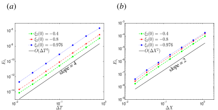
Figure 5: (Color online) Numerical convergence examination of the scheme in time and space. (a) The $l_{1}$ norm error (4.41) as a function of the time step $\Delta T$ under different-amplitude IWs. The green, red, and blue lines correspond to the IW amplitudes $\xi_{2}(0)$ being $-0.4$, $-0.8$, and $-0.976$, respectively. To examine the convergence in time, we use a stopping time $T_{s}=4$ and fix a spatial discretization $\Delta X=600/2^{10}$. The reference solution is computed with a very small time step $\Delta T=0.1/32$. The result in panel (a) shows fourth-order time-accuracy of the scheme. (b) The $l_{1}$ norm error (4.41) as a function of the spatial discretization $\Delta X$ under different-amplitude IWs. To examine the convergence in space, we use a stopping time $T_{s}=1$ and fix the time step $\Delta T=0.01$. The reference solution is computed with $\Delta X=600/2^{16}$. The result in panel (b) shows second-order accuracy in space of the scheme.

Next, we examine the numerical convergence in time and space of our scheme for initially unperturbed interfacial solitary-wave solutions [Eqs. (3.27)-(3.28)]. We compute the $l_{1}$ norm error for the SWs’ profile defined as

$$E_{l_{1}}=\sum_{j}\left|\xi_{1}(X_{j})-\xi_{1}^{\rm ref}(X_{j})\right|\Delta X,$$ (4.41)

where the reference solution $\xi_{1}^{\rm ref}$ is approximated by the numerical result obtained from a very small time step for the time accuracy test or from a very small spatial discretization for the spatial accuracy test. We can see from Fig. 5 that the scheme has fourth-order accuracy in time and second-order accuracy in space.

5 Asymmetric behavior of SWs in the presence of an underlying IW

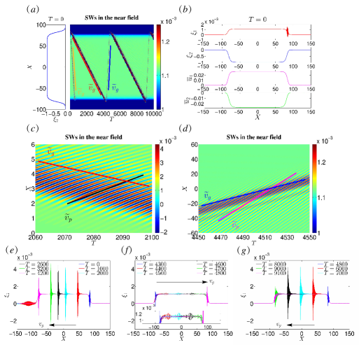
Figure 6: (Color online) (a) Spatiotemporal evolution of SWs’ profile $\xi_{1}$ in the near field for $0\leq T\leq 10000$ and $-100\leq X\leq 100$, and snapshot of the interfacial solitary wave at $T=0$. The amplitude of the interfacial solitary wave is $-0.976$. The yellow line corresponds to the group velocity of the left-moving fast-mode SW packet that is not trapped in the near field. The red (blue) line corresponds to the negative (postive) group velocity, $\widetilde{v}_{g}$, when the right-moving fast-mode SW packet propagates towards the trailing (leading) edge. (b) The initial condition for wave profiles and horizontal velocities $(\xi_{1},\xi_{2},\overline{u}_{1},\overline{u}_{2})$. (c) Zoomed-in version of panel (a) for $2060\leq T\leq 2100$ and $0\leq X\leq 6$. The black line corresponds to the positive phase velocity, $\widetilde{v}_{p}$, and the red line corresponds to the negative group velocity, $\widetilde{v}_{g}$. Wave packets are traveling in the direction of decreasing $X$ towards the trailing edge. (d) Zoomed-in version of panel (a) for $4450\leq T\leq 4550$ and $-60\leq X\leq 60$. The magenta line corresponds to the positive phase velocity, $\widetilde{v}_{p}$, and the blue line corresponds to the positive group velocity, $\widetilde{v}_{g}$. Wave packets are traveling in the direction of increasing $X$ towards the leading edge. (e)(f)(g) Snapshot of SWs in the near field. In panels (e) and (g), the group velocities $v_{g}$ are negative. In panel (f), the group velocity $v_{g}$ is positive.

In this section, we present our numerical results for the system (2.21)-(2.24) describing the behavior of a SW packet in the presence of an underlying interfacial solitary wave, and then compare them to the results of our theoretical analysis using ray-based theories. First, we initialize the SWs’ height $\xi_{1}$ to be a profile composed of a sufficiently-long-wavelength interfacial-solitary-wave solution and a localized perturbation, that is, the initial condition [Fig. 6(b)] for $(\xi_{1},\xi_{2},\overline{u}_{1},\overline{u}_{2})$ is taken to be

$$(\Xi_{1}+\delta_{1},\Xi_{2},\overline{U}_{1},\overline{U}_{2}),$$ (5.42)

where $\left(\Xi_{1},\Xi_{2},\overline{U}_{1},\overline{U}_{2}\right)$ is the solitary-wave solutions described in §§ 3.1 and the localized perturbation $\delta_{1}$ is a narrow SW packet with a narrow band of wavenumbers,

$$\delta_{1}=A_{\varepsilon}[\tanh(X-X_{0}+x_{0})-\tanh(X-X_{0}-x_{0})]\cos(k_{0}(X-X_{0})),$$ (5.43)

with $A_{\varepsilon}=5\times 10^{-4}$, $X_{0}=84$, $x_{0}=2$, and $k_{0}=5$. For the interfacial solitary wave, $\Xi_{2}$, the amplitude is $-0.976$, the wavelength is $\sim 150$, and the speed is $C_{s}=0.0549$.

Below, the group velocity $v_{g}$, the phase velocity $v_{p}$, and the frequency $\nu$ correspond to the moving frame $(T,X)$. On the other hand, the group velocity $c_{g}=(v_{g}+C_{s})$, the phase velocity $c_{p}=(v_{p}+C_{s})$, and the frequency $\omega(=\nu+C_{s}k)$ correspond to the resting frame $(t,x)$. The variable with the tilde, $\widetilde{\cdot}$, stands for the numerical measurement of the corresponding quantity.

Initially, left-moving radiation is quickly emitted from the near field and eventually absorbed by our absorbing boundary condition in the buffer zones [dark stripe parallel to the yellow line in Fig. 6(a)]. After this initial transient, we can see that one SW packet is trapped in the near field [dark stripes parallel to the red line and blue line in Fig. 6(a)]. These trapped waves are all right-moving waves, that is, their phase velocities $\widetilde{v}_{p}>0$ are positive [dark stripes parallel to the black line in Fig. 6(c) and to the magenta line in Fig. 6(d)]. Thus, only the right-moving SWs that propagate in the same direction as the underlying interfacial solitary wave remain trapped in the near field.

We now study the spatiotemporal manifestation of these right-moving SWs in the near field. From Fig. 6, we can observe three features of these right-moving SWs:

(i) SWs become short in wavelength at the leading edge and long at the trailing edge. For $0\leq T\leq 4300$, the SW packets propagate towards the trailing edge with a relatively large wavenumber $\widetilde{k}\sim 23$ [Fig. 6(e)]. For $4300\leq T\leq 4700$, the SW packets propagate towards the leading edge with a relatively small wavenumber $\widetilde{k}\sim 1.8$ [Fig. 6(f)].

(ii) SW packets propagate towards the trailing edge with a relatively small group velocity, and towards the leading edge with a relatively large group velocity. From Figs. 6(a)(c)(e), we can see that for $0\leq T\leq 4300$, the SW packets propagate towards the trailing edge with a relatively small group velocity $\widetilde{v}_{g}\sim-0.045$. For $4300\leq T\leq 4700$ [Figs. 6(a)(d)(f)], the SW packets propagate towards the leading edge with a relatively large group velocity $\widetilde{v}_{g}\sim 0.37$. For $4800\leq T\leq 9100$ [Figs. 6(a)(g)], the SW packets again propagate towards the trailing edge with a relatively small group velocity.

(iii) SWs become high in amplitude at the leading edge and low at the trailing edge. For $0\leq T\leq 4300$, the SW packets’ amplitude increases to $\sim 3\times 10^{-3}$ at the leading edge and then SWs propagate towards the trailing edge [Fig. 6(e)]. For $4300\leq T\leq 4700$, the SW packets’ amplitude decreases to $\sim 1\times 10^{-4}$ at the trailing edge and then propagate towards the leading edge [Fig. 6(f)].

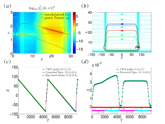
Figure 7: (Color online) (a) The logarithmic modulus, ${\ \log_{10}|\widehat{\xi}_{1}(k,\nu)|^{2}}$, of SWs’ profile $\xi_{1}$ for $3181\leq T\leq 4000$ and $-150\leq X\leq 150$. For comparison, also plotted are the pure linear dispersion relation $\nu_{k}$ (red dashed-dotted curve) and the modulated dispersion relation $\overline{\nu}_{k}$ (black solid curve). The green rectangle corresponds to the range of wavenumbers and frequencies predicted by the ray-based theories [see text and panel (b) for details]. (b) The phase portrait of the motion of wave packets in variables $X$ and $k$. Along each cyan-colored curve, the frequency $\overline{\nu}_{k}$ remains constant. Inside the region enclosed by the blue-level curve, the fast-mode waves are trapped. The red point $P$, $(X,k)=(84,5)$, corresponds to the central location and dominant wavenumber of the perturbation (5.43) and the red-level curve corresponds to the wave passing through the point $P$ with a constant frequency. The distance of two neighboring green points corresponds to the spatial width of the initial perturbation (5.43) and the two green-level curves correspond to the wave passing through the two green points with constant frequencies $\nu=1.46$ and $\nu=1.895$. On these two green-level curves, the maximal wavenumbers are $26.7$ and $15.5$, respectively. For the green rectangle in panel (a), the upper and lower bounds correspond to the two frequencies $\nu=1.46$ and $\nu=1.895$ and the left and right bounds correspond to the wavenumbers $k=26.7$ and $k=15.5$. The arrows indicate the direction of movement of wave packets. (c) The temporal evolution of peak location of the fast-mode waves in the near field. The green curve corresponds to the peak locations of the fast-mode waves from the TWN model (4.35)-(4.38). The blue curve corresponds to the peak locations of the fast-mode waves from the effective linearized equations (1.46)-(1.49) in appendix A. The red curve corresponds to the peak locations of the wave packet predicted by the ray-based theory (5.44)-(5.45). They nearly overlap one another. (d) The temporal evolution of the maximal amplitude, $A$, of the fast-mode waves. The green curve and the blue curve correspond to the height of $A$ for the fast-mode waves of the TWN model (4.35)-(4.38) and those of the effective linearized equations (1.46)-(1.49) in appendix A, respectively. They overlap one another. The time period marked by the red line corresponds to the negative group velocity $v_{g}$ and the black line corresponds to the positive group velocity $v_{g}$. The time period marked by the magenta line corresponds to the positive peak location $X$ and the cyan-line one corresponds to the negative peak location $X$.

To understand the dynamical behavior of these right-moving SWs, we first quantify the dispersion relation of these waves. Figure 7(a) shows the logarithmic modulus, $\log_{10}|\widehat{\xi}_{1}(k,\nu)|^{2}$, with its magnitude color-coded, where $\widehat{\xi}_{1}(k,\nu)$ is the spatiotemporal Fourier transform of $\xi_{1}(X,T)$. For comparison, also shown are the pure linear dispersion relation $\nu_{k}=\omega_{k}-C_{s}k$ [Eq. (3.32), red dashed-dotted curve in Fig. 7(a)] and the modulated dispersion relation $\overline{\nu}_{k}=\overline{\omega}_{k}-C_{s}k$ [Eq. (3.33), black solid curve in Fig. 7(a)]. For the modulated dispersion relation $\overline{\nu}_{k}$, we take the amplitude of the interfacial solitary wave to be $(\Xi_{1},\Xi_{2},\overline{U}_{1},\overline{U}_{2})=(0.001,-0.976,0.027,-0.026)$. We can clearly see from Fig. 7(a) that, for $15\leq k\leq 25$, the modulated dispersion relation $\overline{\nu}_{k}$ can capture the peak locations of the spectrum well, whereas the pure linear dispersion relation $\nu_{k}$ deviates greatly. Therefore, these right-moving SWs can be well characterized by the modulated dispersion relation $\overline{\nu}_{k}$ and thereafter referred to as right-moving fast-mode SWs [see the definition of fast-mode waves in Sec. 3.2].

Incidentally, there are two yellow spots on the pure linear dispersion relation $\nu_{k}$ near $k=5$, as can be observed faintly in Fig. 7(a). However, the spectral power at these two yellow spots on the linear dispersion relation $\nu_{k}$ is six orders of magnitude lower than that at the modulated dispersion relation $\overline{\nu}_{k}$. These two blurry yellow spots correspond to the wave spectra of radiation waves in the far field, which is not the interest of this work.

To understand the asymmetric behavior (i)-(iii), we compare our numerical results of the TWN model with those of the effective linearized equations (1.46)-(1.49) in appendix A. Effective linearized equations (1.46)-(1.49) are obtained from the linearization of our TWN model (4.35)-(4.38) in the presence of the interfacial solitary wave. Their mathematical details are presented in appendix A. We also compare our TWN solutions with the theoretical predictions of ray-based theories. Due to the slow varying in space and time of the phase of fast-mode waves, the governing equations of space-time rays for the location $X$ and the wavenumber $k$ are given by [44, 6],

$$\frac{dX}{dT} =\frac{\partial\overline{\nu}_{k}}{\partial k},$$ (5.44)

$$\frac{dk}{dT} =-\frac{\partial\overline{\nu}_{k}}{\partial X},$$ (5.45)

where $\overline{\nu}_{k}$ is the modulated dispersion relation in Eq. (3.33). Note that the modulated dispersion relation $\overline{\nu}_{k}$ does not explicitly depend on time $T$ since the interfacial solitary wave is stationary in the moving frame. Clearly equations (5.44) and (5.45) constitute a Hamiltonian system with $\overline{\nu}_{k}$ as the Hamiltonian, $X$ displacement and $k$ momentum. Equation (5.44) states that the wave packet propagates at the group velocity.

We now quantify the asymmetric behavior of these right-moving fast-mode SWs by comparing the results of the TWN model, the results of the effective linearized equations, and theoretical predictions from ray-based theories:

(i) First, we provide a theoretical prediction for the temporal evolution of the wavenumber (equivalently the wavelength) of fast-mode waves. By the ray-based theory, when propagating with the initial perturbation (5.43), fast-mode waves possess the peak locations $X$ and wavenumbers $k$ between the two green-level curves in Fig. 7(b). For the minimal wavenumber, the theoretical prediction $k=1.7$ can be attained at $X=0$ on the red-level curve in Fig. 7(b). This theoretical minimal wavenumber is in good agreement with the measured one $\widetilde{k}\sim 1.8$ at $(T,X)=(4500,0)$ in Fig. 6(f). For the maximal wavenumber, the theoretical prediction ranges from $15.5$ to $26.7$ between the two green-level curves in Fig. 7(b). For the theoretical wavenumbers $k=15.5$ and $k=26.7$, the corresponding frequencies are $\nu=1.895$ and $\nu=1.46$, respectively. This range of theoretical wavenumbers and frequencies [depicted by the green rectangle in Fig. 7(a)] is in good agreement with the the range of the measured ones in the spectrum in Fig. 7(a). Therefore, the temporal evolution of the wavenumber can be characterized by the ray-based theory (5.44)-(5.45) for fast-mode waves. In particular, fast-mode SWs become short in wavelength at the leading edge [$X>0$] and long at the trailing edge [$X<0$] [see Fig. 7(b)].

(ii) Next, we investigate the motion of the peak location $X$ as a function of time $T$. Figure 7(c) displays the temporal evolution of numerically measured peak locations of the fast-mode waves for the TWN model (4.35)-(4.38) [green curve in Fig. 7(c)] as well as the prediction using the effective linearized equations (1.46)-(1.49) [blue curve in Fig. 7(c)]. For comparison, also displayed are the peak locations of the wave packets predicted by the ray-based theory (5.44)-(5.45) [red curve in Fig. 7(c)]. One can observe that there is excellent agreement between the numerical results and theoretical predictions for the motion of the peak locations. This confirms that the wave packet moves at the group velocity $v_{g}=\partial\overline{\nu}_{k}/\partial k$. As predicted by the ray-based theory, for $0\leq T\leq 4300$, the group velocity ${v}_{g}\sim-0.045$ is negative with a relatively small magnitude, whereas for $4300\leq T\leq 4700$, the group velocity ${v}_{g}\sim 0.37$ is positive with a relatively large magnitude. These two theoretical group velocities are in excellent agreement with the measured ones, $\widetilde{v}_{g}\sim-0.045$ and $\widetilde{v}_{g}\sim 0.37$, respectively. As reflected in the zig-zag pattern in Fig. 7(c), we can observe that SW packets propagate towards the trailing edge with a relatively small group velocity, and towards the leading edge with a relatively large group velocity.

(iii) Finally, we discuss the temporal evolution of the maximal amplitude, $A$, of fast-mode waves in the near field. Figure 7(d) displays the maximal amplitude of the fast-mode waves in our TWN model (4.35)-(4.38) [green curve] and that predicted using the effective linearized equations (1.46)-(1.49) [blue curve]. One can see very good agreement between them. In addition, one can observe from Fig. 7(d) that the amplitude $A$ is relatively large for the negative group velocity $v_{g}$ (interval marked by the red color), whereas the amplitude $A$ is relatively small for the positive group velocity $v_{g}$ (interval marked by the black color). Furthermore, for $4500\leq T\leq 9300$, the amplitude $A$ grows for positive $X$ (interval marked by the magenta color), whereas it decays for negative $X$ (interval marked by the cyan color). Therefore, SWs become high in amplitude at the leading edge ($X>0$) whereas low at the trailing edge ($X<0$).

To the best of our knowledge, the asymmetric behavior (i) was earlier discovered in references [6, 33], the asymmetric behavior (iii) was earlier discovered in the reference [37], but the asymmetric behavior (ii) was not reported in previous works. Here, we quantify these asymmetric types of behavior predicted by the ray-based theory for our TWN model when the initial perturbation (5.43) is a small-amplitude, narrow-width SW packet with a narrow band of wavenumbers.

6 Conclusions and discussion

Using the long-wavelength and small-amplitude approximations, we have proposed a two-layer, weakly nonlinear (TWN) model (2.21)-(2.24) describing the long-wave interactions between IWs and SWs. The TWN model captures the broadening of large-amplitude IWs that is a ubiquitous phenomenon in the ocean [40, 21]. In Sec. 5, we have investigated the spatiotemporal manifestation and the dynamical behavior of right-moving fast-mode SWs in the near field in the presence of an underlying IW. From our numerical results, the wavenumber, group velocity, and amplitude of fast-mode SW packets of our TWN model (4.35)-(4.38) can always be well captured by the predictions of the effective linearized equations (1.46)-(1.49) and the ray-based theory (5.44)-(5.45). The fast-mode waves behave as linear waves modulated by the underlying interfacial solitary wave. Importantly, the behavior of the right-moving fast-mode waves is asymmetric at the leading edge vs. the trailing edge when an underlying IW is present:

(i) SWs become short in wavelength at the leading edge and long at the trailing edge [Fig. 7(b)].

(ii) SW packets propagate towards the trailing edge with a relatively small group velocity, and towards the leading edge with a relatively large group velocity [Fig. 7(c)].

(iii) SWs become high in amplitude at the leading edge and low at the trailing edge [Fig. 7(d)].

In this work, we only focus on the spatiotemporal manifestation and dynamical behavior of SWs under a small-amplitude initial perturbation. As a natural extension of the above results, it is interesting to study the SWs when the amplitude of the perturbation is large, that is, the nonlinearity becomes prominent. In particular, it is important to understand how the nonlinearity and resonance affect the spatiotemporal manifestation and dynamical behavior of the right-moving fast-mode SWs in the presence of an underling IW.

Class 3 triad resonance is believed to be responsible for the surface signature of the underlying internal waves [38, 35, 29, 17]. The TWN model possesses two-mode waves, one slow and the other fast, and thus resonant interactions among different modes can occur during the energy exchange process [more details can be found in Appendix B]. The class 3 triad resonance condition [Eq. (2.50) in Appendix B], $c_{g}(k)=C_{p}(0)$, shows that, for resonantly-interacting waves, the group velocity of fast-mode waves $c_{g}(k)$ and the phase velocity of slow-mode waves $C_{p}(0)$ are equal [41, 27]. From many field observations, a narrow band of SWs with the resonant wavenumber was found to be located at the leading edge of an underlying IW and travel nearly at the same speed as the underlying IW [38, 35]. The surface phenomena may be related to both the triad resonance excitation and the three asymmetric types of behavior (i)-(iii). The allowance of triad resonance in the TWN model encourages us to investigate the spatiotemporal manifestation and dynamical behavior of SWs under large-amplitude initial perturbations in future work.

7 Acknowledgements

This work is supported by NYU Abu Dhabi Institute G1301, NSFC Grant No. 11671259, 11722107, and 91630208, and SJTU-UM Collaborative Research Program (D.Z.). We dedicate this paper to our late mentor David Cai.

Appendix A Effective linearized equations

In this section, we present the effective linearized equations of the TWN model (4.35)-(4.38). The variables $(\xi_{i},\overline{u}_{i})$ in the TWN model are composed of two components, one being the interfacial solitary wave $(\Xi_{i},\overline{U}_{i})$ and the other the perturbation of fast-mode waves $(\widehat{\xi}_{i},\widehat{\overline{u}}_{i})$. By substituting $(\xi_{i},\overline{u}_{i})=(\Xi_{i},\overline{U}_{i})+(\widehat{\xi}_{i},\widehat{\overline{u}}_{i})$ into the system (4.35)-(4.38) and collecting the linear terms with respect to $(\widehat{\xi}_{i},\widehat{\overline{u}}_{i})$, we can obtain the effective linearized equations for the fast-mode waves as follows,

$$\widehat{\eta}_{1T}-C_{s}\widehat{\eta}_{1X}+\left[H_{1}\widehat{\overline{u}}_{1}+\overline{U}_{1}(\widehat{\xi}_{1}-\widehat{\xi}_{2})\right]_{X}=0,$$ (1.46)

$$\widehat{\eta}_{2T}-C_{s}\widehat{\eta}_{2X}+(H_{2}\widehat{\overline{u}}_{2}+\overline{U}_{2}\widehat{\xi}_{2})_{X}=0,$$ (1.47)

$$\widehat{M}_{1T}-C_{s}\widehat{M}_{1X}+\left(\overline{U}_{1}\widehat{\overline{u}}_{1}+g\widehat{\xi}_{1}\right)_{X}=0,$$ (1.48)

$$\widehat{M}_{2T}-C_{s}\widehat{M}_{2X}+\left(\overline{U}_{2}\widehat{\overline{u}}_{2}+g\widehat{\xi}_{2}+\rho_{r}g\widehat{\eta}_{1}\right)_{X}=0,$$ (1.49)

where

$$H_{1}=h_{1}+\Xi_{1}-\Xi_{2},\text{ \ \ }H_{2}=h_{2}+\Xi_{2},$$

$$\widehat{\eta}_{1}=h_{1}+\widehat{\xi}_{1}-\widehat{\xi}_{2},\text{ \ \ }\widehat{\eta}_{2}=h_{2}+\widehat{\xi}_{2},$$

$$\widehat{M}_{1}=\widehat{\overline{u}}_{1}-\frac{1}{3}h_{1}^{2}\widehat{\overline{u}}_{1XX}-\frac{1}{2}h_{1}\left(H_{2}\widehat{\overline{u}}_{2}+\overline{U}_{2}\widehat{\xi}_{2}\right)_{XX},$$

$$\widehat{M}_{2}=\widehat{\overline{u}}_{2}-\frac{1}{2}\rho_{r}h_{1}^{2}\widehat{\overline{u}}_{1XX}-\frac{1}{3}h_{2}^{2}\widehat{\overline{u}}_{2XX}-\rho_{r}h_{1}\left(H_{2}\widehat{\overline{u}}_{2}+\overline{U}_{2}\widehat{\xi}_{2}\right)_{XX}.$$

Appendix B Class 3 triad resonance condition

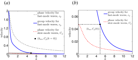
Figure 8: (Color online) (a) Comparison of the phase velocity for fast-mode waves $c_{p}$ , the group velocity for fast-mode waves $c_{g}$, and the phase velocity for slow-mode waves $C_{p}$, with the parameters $(h_{1},h_{2},g,\rho_{1},\rho_{2})=(1,3,1,1,1.003)$. The resonant wavenumber $k_{\mathrm{res}}$ satisfies the triad resonance condition (2.50) (b) Zoomed-in version of panel (a).

In this section, we briefly verify the existence of solutions to the three-wave-resonance condition in the TWN model. If the dispersion relation allows the wavenumbers $k_{i}\ (i=1,2,3)$ and the corresponding frequencies $\omega_{k}(k_{1})$, $\omega_{k}(k_{2})$, and $\Omega_{k}(k_{1})$ to satisfy the conditions,

$$k_{1} -k_{2}=k_{3},$$

$$\omega_{k}(k_{1}) -\omega_{k}(k_{2})=\Omega_{k}(k_{3}),$$

these three waves constitute a class 3 resonant triad. Moreover, if the wavenumbers are specified as $k_{1}=k+\Delta k/2$, $k_{2}=k-\Delta k/2$, $k_{3}=\Delta k$, where $\Delta k\ll k$ and $\Delta k\rightarrow 0$, then the resonance condition reduces to

$$c_{g}(k)=C_{p}(0),$$ (2.50)

where the group velocity $c_{g}$ and the phase velocity $C_{p}$ are given by the equations

$$c_{g}(k)\equiv\frac{\partial\omega_{k}\left(k\right)}{\partial k},\ \ \ \ C_{p}(0)\equiv\left.\frac{\Omega_{k}(\Delta k)}{\Delta k}\right|_{\Delta k\rightarrow 0}.$$ (2.51)

Here, $\omega_{k}$ corresponds to the dispersion relation of fast-mode waves in Eq. (3.32), and $\Omega_{k}$ corresponds to the dispersion relation of slow-mode waves in Eq. (3.31). Many early results [41, 27, 16, 17, 1] have confirmed that there exists a unique resonant wavenumber, denoted by $k_{\text{res}}$, satisfying Eq. (2.50) in the two-layer fluid system. For the TWN model, one can observe from Fig. 8 that there exists a unique resonant wavenumber $k_{\text{res}}$, satisfying the resonance condition (2.50), $c_{g}(k_{\text{res}})=C_{p}(k=0)$. Therefore, class 3 resonant triads exist among two fast-mode waves and one slow-mode wave for the TWN model.

References

- [1] Mohammad-Reza Alam. A new triad resonance between co-propagating surface and interfacial waves. J. Fluid Mech., 691:267–278, 2012.
- [2] Mohammad-Reza Alam, Yuming Liu, and Dick KP Yue. Bragg resonance of waves in a two-layer fluid propagating over bottom ripples. part i. perturbation analysis. J. Fluid Mech., 624:191–224, 2009.
- [3] M. H. Alford, T. Peacock, J. A. MacKinnon, J. D. Nash, M. C. Buijsman, L. R. Centuroni, S.-Y. Chao, M.-H. Chang, D. M. Farmer, O. B. Fringer, et al. The formation and fate of internal waves in the south china sea. Nature, 521(7550):65–69, 2015.
- [4] D Ambrosi. Hamiltonian formulation for surface waves in a layered fluid. Wave motion, 31(1):71–76, 2000.
- [5] J. R. Apel, L. A. Ostrovsky, Y. A. Stepanyants, and J. F. Lynch. Internal solitons in the ocean and their effect on underwater sound. J. Acoust. Soc. Amer., 121(695 C722), 2007.
- [6] V. V. Bakhanov and L. A. Ostrovsky. Action of strong internal solitary waves on surface waves. J. Geophys. Res., 107(3139), 2002.
- [7] R. Barros and W. Choi. Inhibiting shear instability induced by large amplitude internal solitary waves in two-layer flows with a free surface. Stud. Appl. Math, 122(325-346), 2009.
- [8] R. Barros and S. Gavrilyuk. Dispersive nonlinear waves in two-layer flows with free surface part ii. large amplitude solitary waves embedded into the continuous spectrum. Stud. Appl. Math, 119(213-251), 2007.
- [9] E. A. Caponi, D. R. Crawford, H. C. Yuen, and P. G. Saffman. Modulation of radar backscatter from the ocean by a variable surface current. Technical report, DTIC Document, 1988.
- [10] Tong Chen. An efficient algorithm based on quadratic spline collocation and finite difference methods for parabolic partial differential equations. PhD thesis, University of Toronto, 2005.
- [11] W. Choi, R. Barros, and T.-C. Jo. A regularized model for strongly nonlinear internal solitary waves. J. Fluid Mech., 629(73-85), 2009.
- [12] W. Choi and R. Camassa. Weakly nonlinear internal waves in a two-fluid system. J. Fluid Mech., 313(83-103), 1996.
- [13] W. Choi and R. Camassa. Fully nonlinear internal waves in a two-fluid system. J. Fluid Mech., 396(1-36), 1999.
- [14] W. Craig, P. Guyenne, and H. Kalisch. A new model for large amplitude long internal waves. C. R. Mecanique, 332(525-530), 2004.
- [15] W. Craig, P. Guyenne, and H. Kalisch. Hamiltonian long wave expansions for free surfaces and interfaces. Commun. Pure Appl. Maths, 58(1587-1641), 2005.
- [16] W. Craig, P. Guyenne, and C. Sulem. Coupling between internal and surface waves. Nat. Hazards, 57(617-642), 2011.
- [17] W. Craig, P. Guyenne, and C. Sulem. The surface signature of internal waves. J. Fluid Mech., 710(277-303), 2012.
- [18] F. Dias and A. Il’ichev. Interfacial waves with free-surface boundary conditions: an approach via a model equation. Physica D, 150(278-300), 2001.
- [19] A. N. Donato, D. H. Peregrine, and J. R. Stocker. The focusing of surface waves by internal waves. J. Fluid Mech., 384:27–58, 1999.
- [20] T. F. Duda and D. M. Farmer. The 1998 WHOI/IOS/ONR Internal Solitary Wave Workshop: Contributed Papers. Technical report, DTIC Document, 1999.
- [21] T. F. Duda, J. F. Lynch, J. D. Irish, R. C. Beardsley, S. R. Ramp, C. S. Chiu, T. Y. Tang, and Y. J. Yang. Internal tide and nonlinear wave behavior in the continental slope in the northern south china sea. IEEE J. Ocean. Eng., 29(1105-1131), 2004.
- [22] C. Fochesato, F. Dias, and R. Grimshaw. Generalized solitary waves and fronts in coupled korteweg-de vries systems. Physica D, 210(96-117), 2005.
- [23] M. Funakoshi and M. Oikawa. The resonant interaction between a long internal gravity wave and a surface gravity wave packet. J. Phys. Soc. Jpn, 56(1982-1995), 1983.
- [24] A. E. Gargett and B. A. Hughes. On the interaction of surface and internal waves. J. Fluid Mech., 52(01):179–191, 1972.
- [25] Philippe Guyenne. Large-amplitude internal solitary waves in a two-fluid model. Comptes Rendus Mécanique, 334(6):341–346, 2006.
- [26] H. Han and Z. Xu. Numerical solitons of generalized korteweg cde vries equations. Appl. Math. Comput., 186(483-489), 2007.
- [27] Y. Hashizume. Interaction between short surface waves and long internal waves. J. Phys. Soc. Jpn, 48(631-638), 1980.
- [28] K. R. Helfrich and W. K. Melville. Long nonlinear internal waves. Annu. Rev. Fluid Mech., 38(395-425), 2006.
- [29] H.-H. Hwung, R.-Y. Yang, and I. V. Shugan. Exposure of internal waves on the sea surface. J. Fluid Mech., 626(1-20), 2009.
- [30] Christopher R Jackson and J Apel. An atlas of internal solitary-like waves and their properties. Contract, 14(03-C):0176, 2004.
- [31] T.-C. Jo and W. Choi. On stabilizing the strongly nonlinear internal wave model. Stud. Appl. Math, 120(65-85), 2008.
- [32] Takuji Kawahara, Nobumasa Sugimoto, and Tsunehiko Kakutani. Nonlinear interaction between short and long capillary-gravity waves. J. Phys. Soc. Jpn., 39(5):1379–1386, 1975.
- [33] Tsubasa Kodaira, Takuji Waseda, Motoyasu Miyata, and Wooyoung Choi. Internal solitary waves in a two-fluid system with a free surface. J. Fluid Mech., 804:201–223, 2016.
- [34] C Gary Koop and Gerald Butler. An investigation of internal solitary waves in a two-fluid system. J. Fluid Mech., 112:225–251, 1981.
- [35] R. A. Kropfli, L. A. Ostrovski, T. P. Stanton, E. A. Skirta, A. N. Keane, and V. Irisov. Relationships between strong internal waves in the coastal zone and their radar and radiometric signatures. J. Geophys. Res., 104(3133-3148), 1999.
- [36] K.-J. Lee, I. V. Shugan, and J.-S. An. On the interaction between surface and internal waves. J. Korean Phys. Soc., 51(616-622), 2007.
- [37] J. E. Lewis, B. M. Lake, and D. R. S. Ko. On the interaction of internal waves and surface gravity waves. J. Fluid Mech., 63(04):773–800, 1974.
- [38] A. R. Osborne and T. L. Burch. Internal solitons in the andaman sea. Science, 208(451-460), 1980.
- [39] E. Parau and F. Dias. Interfacial periodic waves of permanent form with free-surface boundary conditions. J. Fluid Mech., 437(325-336), 2001.
- [40] R. B. Perry and G. R. Schimke. Large-amplitude internal waves observed off the northwest coast of sumatra. J. Geophys. Res., 70(10):2319–2324, 1965.
- [41] O. M. Phillips. Nonlinear dispersive waves. Annu. Rev. Fluid Mech., 6(93-110), 1974.
- [42] N. Sepulveda. Solitary waves in the resonant phenomenon between a surface gravity wave packet and an internal gravity wave. Phys. Fluids, 30(7), 1987.
- [43] M. Tanaka and K. Wakayama. A numerical study on the energy transfer from surface waves to interfacial waves in a two-layer fluid system. J. Fluid Mech., 763:202–217, 2015.
- [44] G. B. Whitham. Linear and Nonlinear Waves. A Wiley-Interscience Publication, New York, 1974.