Real-bogus classification for the Zwicky Transient Facility using deep learning

Abstract

Efficient automated detection of flux-transient, reoccurring flux-variable, and moving objects is increasingly important for large-scale astronomical surveys. We present braai, a convolutional-neural-network, deep-learning real/bogus classifier designed to separate genuine astrophysical events and objects from false positive, or bogus, detections in the data of the Zwicky Transient Facility (ZTF), a new robotic time-domain survey currently in operation at the Palomar Observatory in California, USA. Braai demonstrates a state-of-the-art performance as quantified by its low false negative and false positive rates. We describe the open-source software tools used internally at Caltech to archive and access ZTF’s alerts and light curves (Kowalski), and to label the data (Zwickyverse). We also report the initial results of the classifier deployment on the Edge Tensor Processing Units (TPUs) that show comparable performance in terms of accuracy, but in a much more (cost-) efficient manner, which has significant implications for current and future surveys.

1 Introduction and context

Astronomical sky surveys observe a plethora of transient events in the dynamic sky originating from a wide range of astrophysical objects and processes. Detection of such events can be performed in the catalog domain (e.g., CRTS survey; Drake et al. (2009)) and/or in the image domain (e.g., PTF survey; Law et al. (2009)). In the latter case, an epochal image of a patch of the sky is compared to a reference image, which is usually achieved by means of image subtraction. In the process, time-dependent characteristics of the images such as the point spread functions (PSF) and depth are matched. There are multiple factors that may lead to false positive, or bogus, detections in the resulting subtracted images:

• Unmodeled differences between the images that are present even in the idealized situation of noise absence, e.g. radiation hits, optical ghosts, persistent charge, and imperfections in flat-fielding.

• Noise and, most importantly, its unmodeled components, e.g. registration errors, source noise errors, and incorrect estimates of the noise components.

Current and future large-scale surveys have the ability to detect millions of subtraction residuals a night, manifesting the need for automated separation of genuine astrophysical events from bogus detections. Both the real and bogus events may be caused by a wide variety of phenomena, some of which are very hard to model. For example, there is no proper statistical model for radiation hits and optical ghosts. Therefore, an explicit programmatic solution to the problem is difficult and it is most efficient to apply machine learning (ML) methods to extract the relevant patterns from the data themselves.

The real/bogus (RB) ML classifiers score individual sources on a scale from 0.0 (bogus) to 1.0 (real). RB classifiers were first introduced by Bailey et al. (2007) for the Nearby Supernova Factory (Aldering et al., 2002), and have been adopted by other time domain surveys including the Palomar Transient Factory (PTF; Bloom et al., 2008) and the Intermediate Palomar Transient Factory (iPTF; Brink et al., 2012; Wozniak et al., 2013; Rebbapragada et al., 2015), the Dark Energy Survey (Goldstein et al., 2015), Pan-STARRS (Wright et al., 2015), and HiTS (Cabrera-Vives et al., 2017; Reyes et al., 2018).

The Zwicky Transient Facility

The Zwicky Transient Facility (ZTF) is a new robotic time-domain sky survey capable of visiting the entire visible sky north of $-30^{\circ}$ declination every night. ZTF observes the sky in the $g$, $r$, and $i$ bands at different cadences depending on the scientific program and sky region (Bellm et al., 2019; Graham et al., 2019). The new 576 megapixel camera with a 47 deg² field of view, installed on the Samuel Oschin 48-inch (1.2-m) Schmidt Telescope, can scan more than 3750 deg² per hour, to a $5\sigma$ detection limit of 20.7 mag in the $r$ band with a 30-second exposure during new moon (Dekany & Smith, 2019; Masci et al., 2019).

The raw data are transferred to the Infrared Processing and Analysis Center (IPAC) at the California Institute of Technology (Caltech) and processed in real time. The ZTF Science Data System (ZSDS) housed at IPAC consists of the data processing pipelines, data archives, infrastructure for long-term curation, and the services for data retrieval and visualization. For the detailed description of the ZSDS please refer to Masci et al. (2019).

The part of the ZSDS responsible for the transient event detection and extraction, first “properly” subtracts a reference (template) image from a calibrated science exposure image. In summary, this step involves using a subset of sources from the input reference and epochal (science) PSF-fit photometry catalogs to match the photometric throughputs of the corresponding images; resamples and interpolates the reference image onto the science image using SWarp (Bertin, 2010); masks all bad pixels propagated from the science and reference images; computes a smoothly varying differential background image and subtracts this from the science image. Pixel-uncertainty images and PSFs for the science and reference images are then generated. PSF matching and image differencing are then performed using the ZOGY algorithm (Zackay et al., 2016).

If the resulting difference image is of sufficient quality, the pipeline then detects events from the point-source match-filtered S/N images where detection is performed on both the positive (science minus reference) and negative (reference minus science) images. Events are extracted with both aperture and PSF-fit photometry, and additional source features are computed. The events are then lightly filtered to remove obvious false positives and image cutouts are generated (Masci et al., 2019).

Events may have been triggered from a flux-transient, a reoccurring flux-variable, or a moving object. The metadata and contextual information including the cutouts are put into “alert packets” that are further picked up by the ZTF Alert Distribution System (ZADS). On a typical night, the number of detected events ranges from $10^{5}$ – $10^{6}$.

The RB classifier initially employed by ZTF heavily relied on the PTF/iPTF legacy and was built using the random forest (RF) algorithm. To make a prediction, it used the source features extracted from the science and subtracted image cutouts centered on the candidate, supplemented with other measurements taken from the science, subtracted, and reference images. Please refer to Mahabal et al. (2019) and Rebbapragada et al. (in prep.) for the details on the RF RB classifier.

In this paper, we present braai, a new cutout-image-based RB classifier built for ZTF using deep learning (DL) that demonstrates a state-of-the-art performance, superior compared to the original RF classifier. Additionally, we describe the open-source software tools used internally at Caltech to archive and access ZTF’s alerts and light curves (Kowalski), and to label the data (Zwickyverse).

2 braai: a Deep Learning framework for real-bogus classification

Deep learning is a subset of ML that employs artificial many-layer neural networks (McCulloch & Pitts, 1943). DL systems are able to discover, in a highly automated manner, efficient representations of the data, simplifying the task of finding the meaningful sought-after patterns in them.

2.1 Data set

DL systems are able to learn even very complicated, highly non-linear mappings between the input and output spaces reaching near-optimal performance. The challenge is to construct a large, labelled, representative data set for the network training. In case of the RB classification, the training set must reflect the possible variations across different filters, sky location, CCDs, as well as cross-talk.

In this work, we used a number of sources for data collection. The ZADS distributes the alert packets in the Apache Avro^TM format through the ZSDS Kafka cluster at IPAC (Masci et al., 2019).

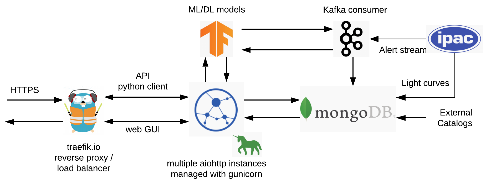
Figure 1: Architecture of Kowalski. See Section 2.1.1 for a detailed description.

Internally at Caltech, the alert stream is consumed by Kowalski, an open-source system primarily used to archive and access ZTF’s alerts and light curves (see Section 2.1.1). We queried Kowalski to gather samples of data representing the vast diversity of ZTF’s alert parameter space.

Another internal consumer, the GROWTH Marshal (Kasliwal et al., 2019), is used to analyze and coordinate follow-up of the sources discovered in the ZTF alert stream through programmatic filtering and human vetting. The GROWTH marshal served as the primary source of pre-labelled (mostly transient) events.

A large number of the bogus examples was collected at the start of the survey for the RF classifier since the initial focus was to filter out the majority of the typical artifacts present in the alert stream such as those caused by the bright stars.

Finally, a small chunk of pre-labelled data came from the Zooniverse Citizen Science platform, where we set up a dedicated project (see https://www.zooniverse.org/projects/rswcit/zwickys-quirky-transients). These data were used for testing purposes (see Section 3.1).

2.1.1 Kowalski

We developed Kowalski for the primary task of supporting the time-domain astronomy efforts with ZTF. Concretely, it solves the problem of efficient storage and access (both programmatic and GUI-based) through a standardized application programming interface (API) to both ZTF’s alert/light-curve data and external catalogs.

Kowalski’s architecture is shown in Fig. 1. The back-end is powered by a non-relational (NoSQL) database MongoDB with an API layer on top of it managing the incoming and outgoing traffic/data streams. We based the choice of MongoDB as the workhorse on the following reasons:

• Individual entries are stored as binary JSON (BSON) “documents” in “collections”. This naturally maps to the format of the alert AVRO packets. The light curve data are stored per source, thus significantly reducing the number of necessary read operations when accessing the data.

• Collections are implemented as B-trees, which guarantees $\sim log(N)$ execution times for the standard database CRUD (create, read, update and delete) operations, where $N$ is the number of documents in the collection.

• Collections support multiple, potentially compound indexes and associated (frequently, in-memory) “covered” queries, providing efficient access to the most-in-demand data.

• Being a NoSQL database, MongoDB does not enforce any schema by default meaning no downtime in case of an alert packet schema change.

• Built-in GeoJSON support with 2D indexes on the sphere allowing efficient, potentially complicated positional queries.

• Built-in support for horizontal scaling through sharding.

The API layer is built using a python asynchronous web framework aiohttp. Authorization is performed using the JSON web tokens. The standard python async event loop (with futures scheduling) serves as a simple, fast, and robust job queue. Both web-based graphical user interface (GUI) and a programmatic python client are available to interact with the API in a standardized manner. Multiple instances of the server app are maintained using the gunicorn process manager. The API supports a range of MongoDB Query Language (MQL)-based queries such as cone and general searches, map-reduce, and aggregation pipelines.

A dedicated Kafka consumer listens to the ZTF alert stream at IPAC and saves it to the database. It has the ability to filter and annotate the alerts prior to database ingestion (by e.g. evaluating ML models).

We choose to use traefik as the reverse proxy/load balancer for its simplicity, performance, and encryption (TLS) support out-of-the-box.

Kowalski is containerized using the Docker software allowing for simple and efficient deployment in the cloud and/or on-premises.

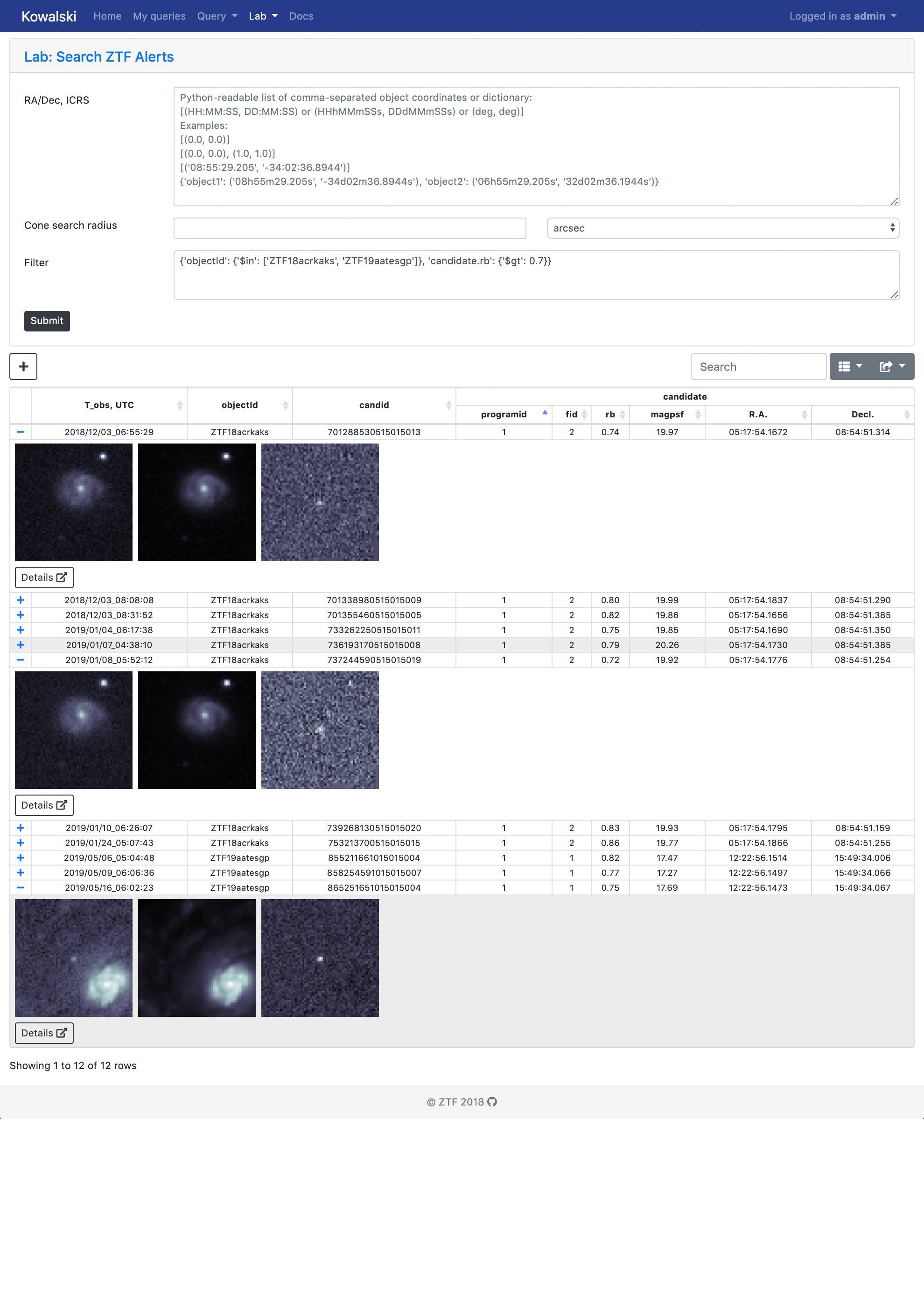
(a) Search interface page

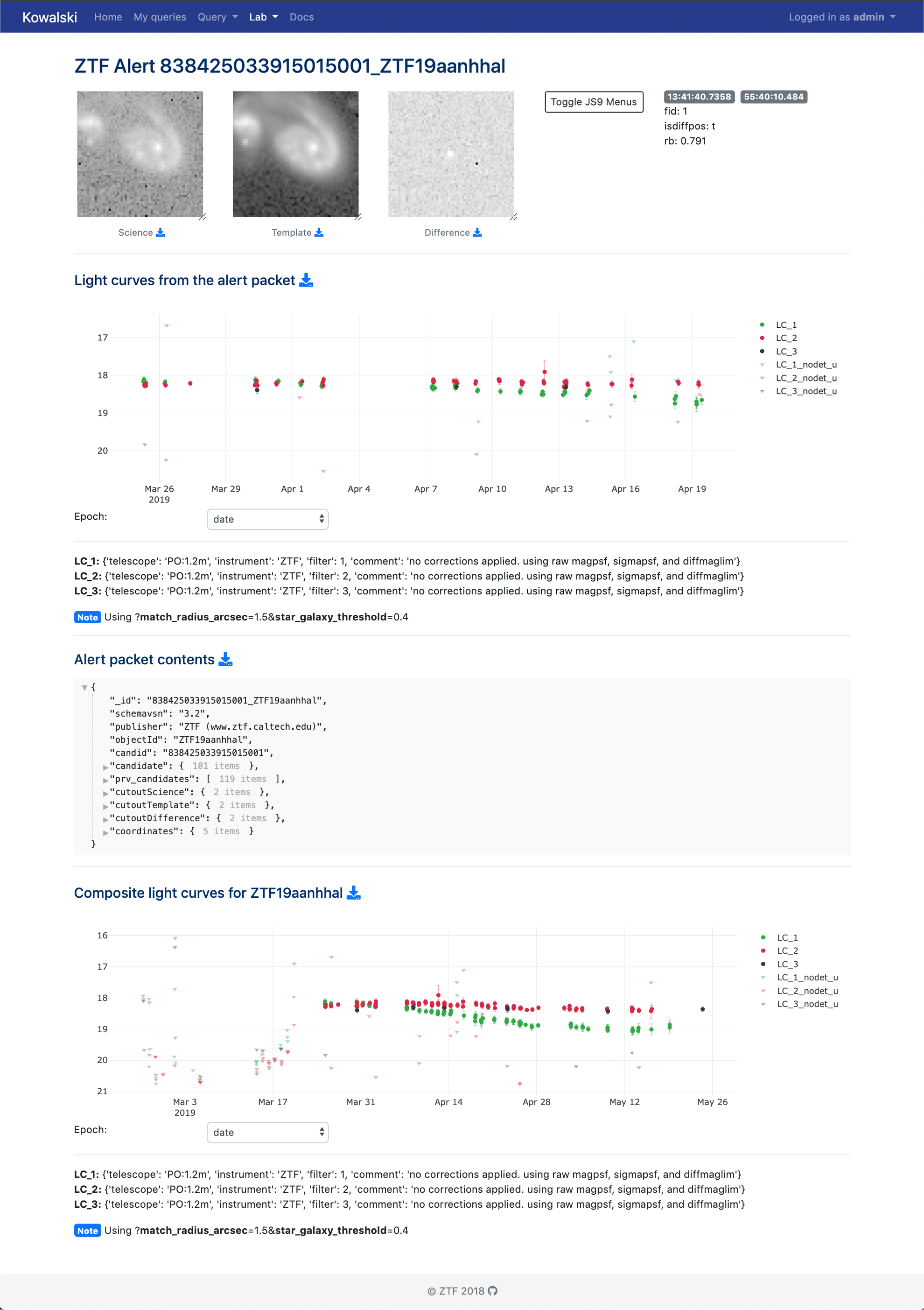
(b) Individual alert page

Figure 2: Kowalski’s ZTF Alert Lab GUI.

To simplify access to the ZTF alert data, Kowalski has a web-based GUI called the ZTF Alert Lab (ZAL), where users can efficiently search and preview alert contents (see Fig. 2a). The ZAL also provides detailed views of individual alerts, interactively displaying the image cutouts (with JS9), alert contents, and the light curves (see Fig. 2b). The latter may be corrected for the flux present in the reference (template) images.

Additionally, the ZAL is able to construct compound object light curves since, due to packet size considerations, the individual alerts only contain a rolling 30-day window with historical data points.

As of June 2019, an instance of Kowalski deployed on-premises at Caltech stores over $30$ TB of various catalogs and databases including $125M+$ alerts and $2.5B+$ light curves. It processes millions of requests daily from $40+$ users, both programmatic services (e.g. ZTF’s transient, variable, and Solar system marshals) and astronomers.

2.1.2 Data labelling

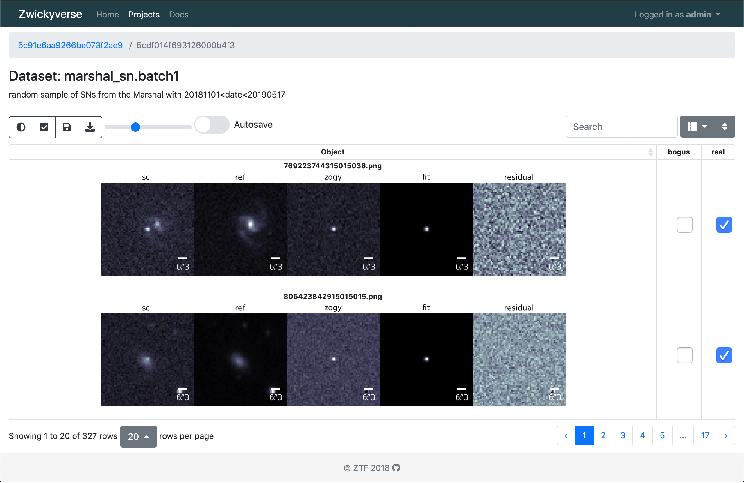
Figure 3: Zwickyverse’s GUI with sample image quintets (science, reference, difference, 2D-Moffat fit of difference, and 2D-Moffat fit minus difference residual)

For data labeling, we used a simple web-based open-source tool called Zwickyverse that provides both an efficient API and GUI. The tool is easy to deploy thanks to containerization using Docker software and it allows quick integration of newly-labelled data sets into the model training workflow. All data labelling for this work was done using Zwickyverse.

To simplify labeling the image cutout triplets (science, reference, difference), we fitted the PSFs in the difference images by 2D-Moffat functions and plotted those together with residual images (difference minus fit, see Fig. 3). This proved to be helpful in identifying certain bogus detections. Additionally, contentious examples were individually inspected using the ZAL.

2.1.3 Data diversity

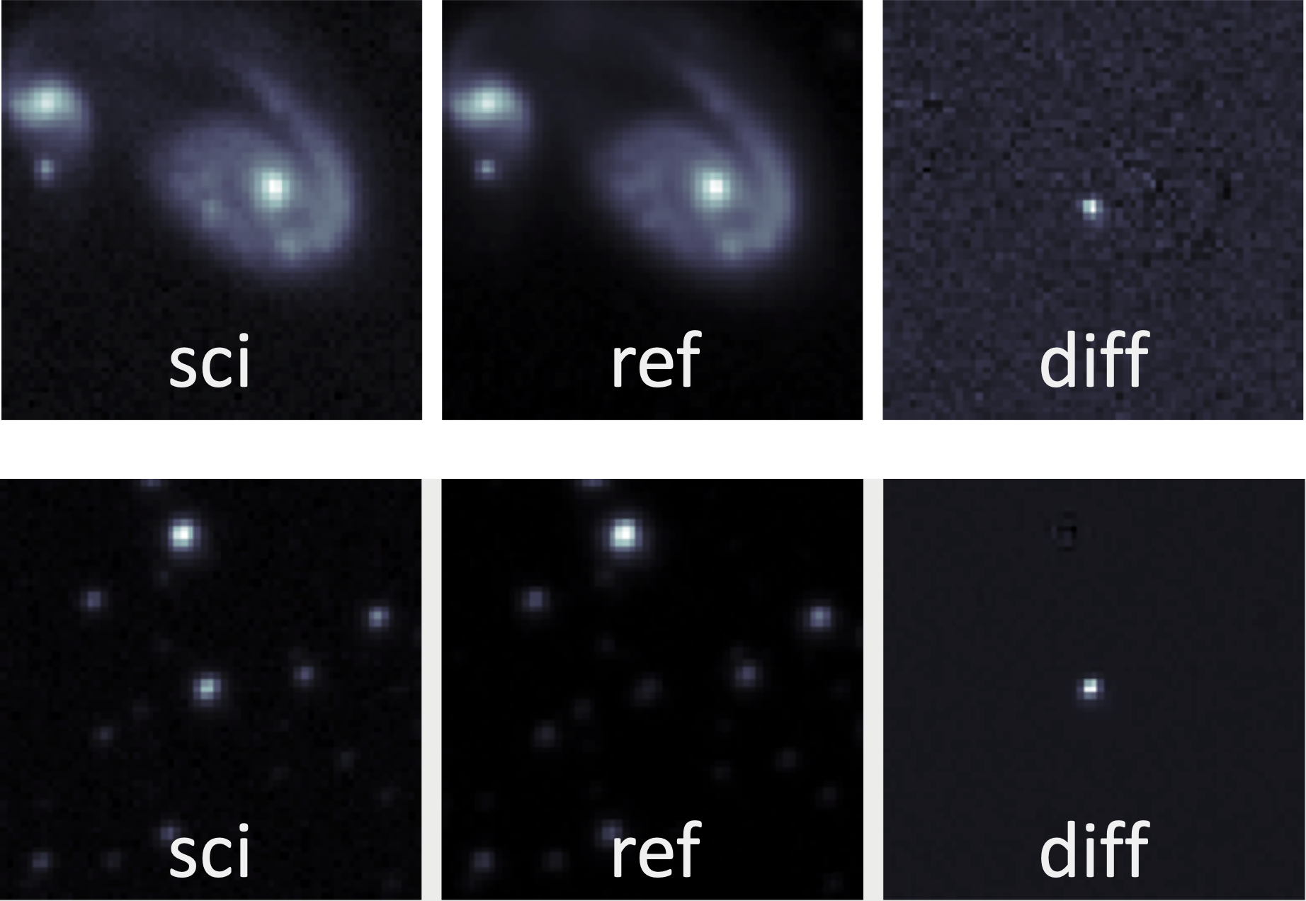
(a) Real examples: a supernova (top) and a variable star (bottom)

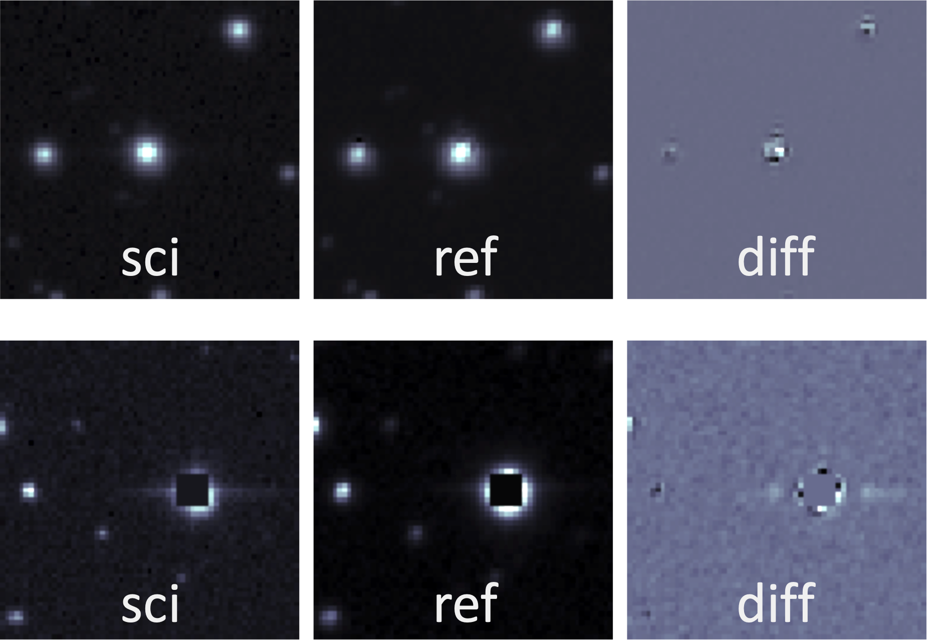
(b) Bogus examples: a badly-subtracted star (top) and an artifact caused by a masked bright object

Figure 4: Examples of 63x63 pixel cutout image triplets (science, reference, difference). ZTF plate scale is $1\arcsec$ per pixel.

We strove to build a data set that adequately samples the ZTF alert parameter space. For that, we collected over thirty thousand training examples with the real-to-bogus data ratio of about $55\%/45\%$ (see Fig. 4). Fig. 5 shows the histograms of example counts as functions of the date and several candidate source characteristics extracted from the difference image: full width at half maximum (FWHM), PSF magnitude, and signal-to-noise ratio (SNR). Fig. 6 shows the training set breakdown by filters, position in/out of the Galactic plane, and positive vs. negative subtractions. There are certain imbalances in the data set and we are planning to mitigate them in the future.

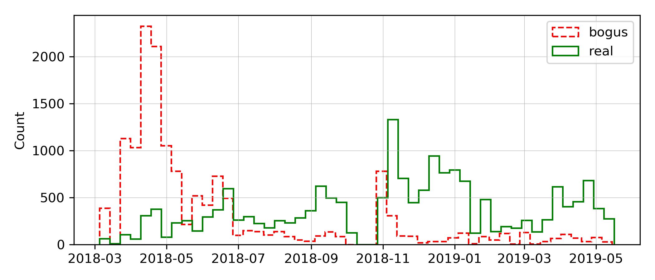
(a) Date

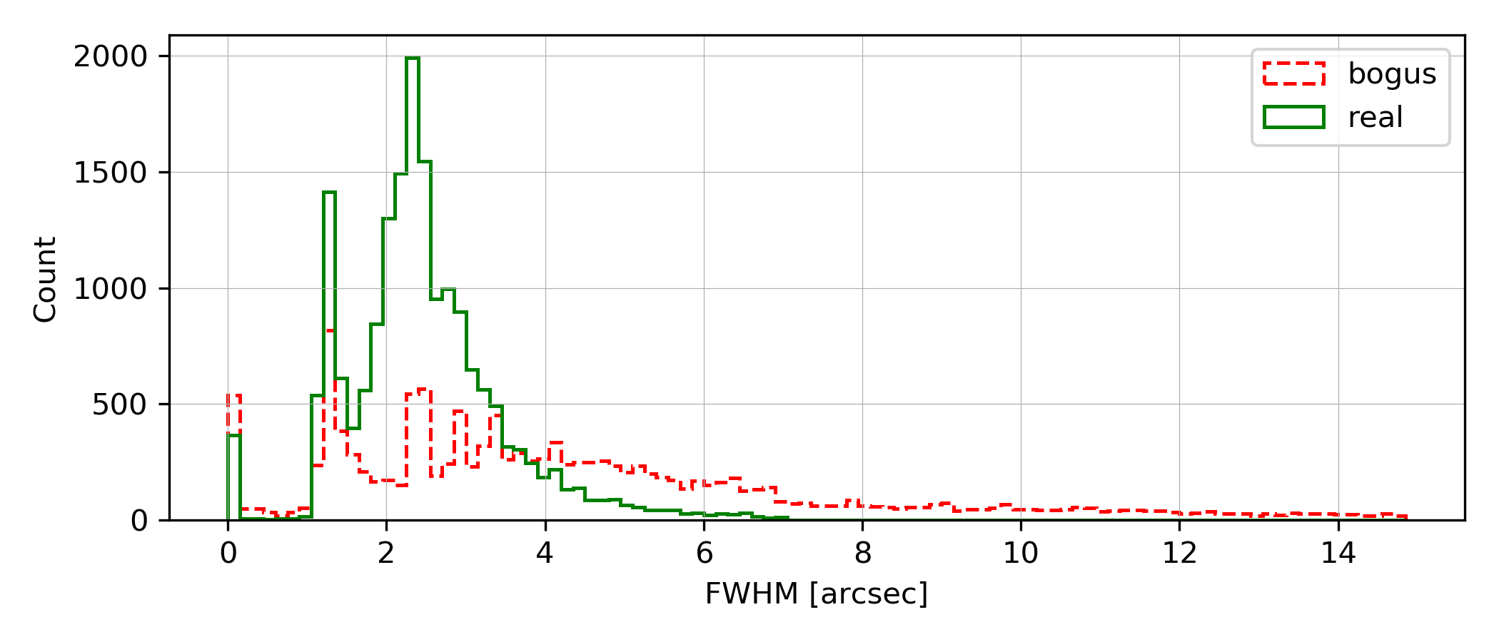
(b) FWHM

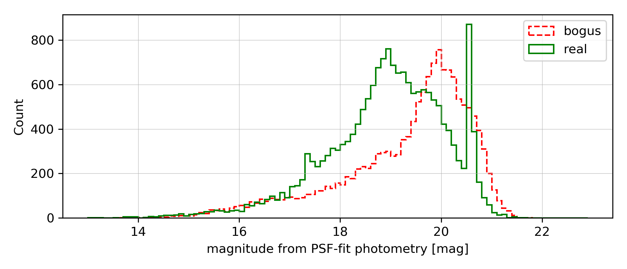
(c) PSF magnitude

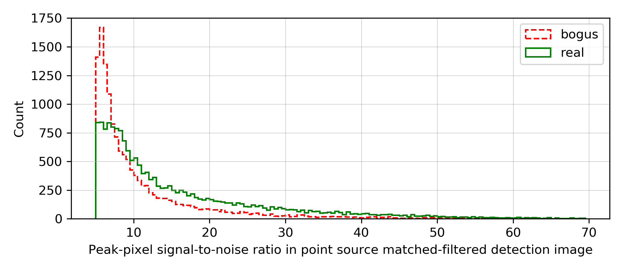
(d) SNR

Figure 5: Training data breakdown by date, full width at half maximum (FWHM), PSF magnitude in the difference image, and peak-pixel signal-to-noise ratio in point source matched-filtered detection image. Most of the sharp peaks on the histograms are due to selection effects. The peak at zero on the FWHM histogram is due to a data processing artifact, which was fixed in May, 2018.

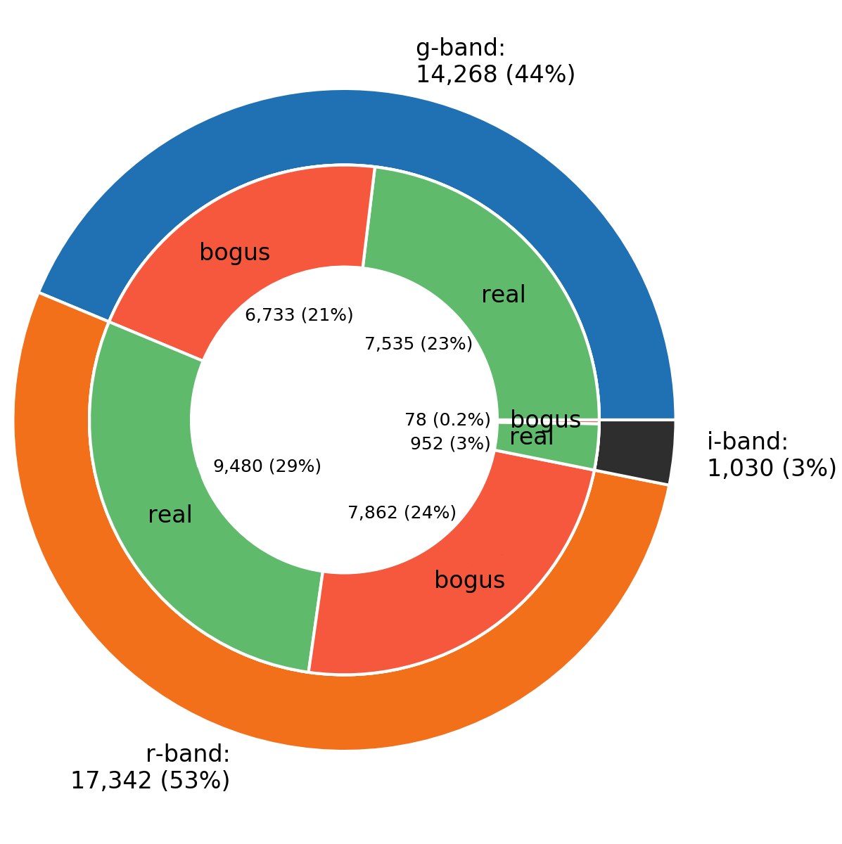
(a) Filters

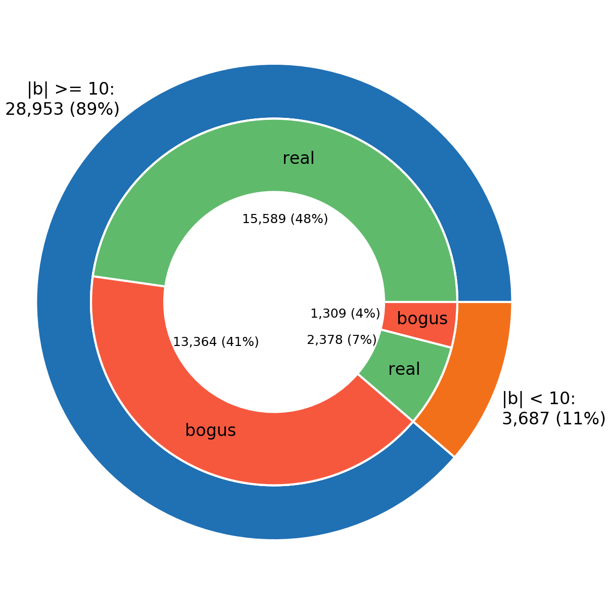
(b) Galactic plane

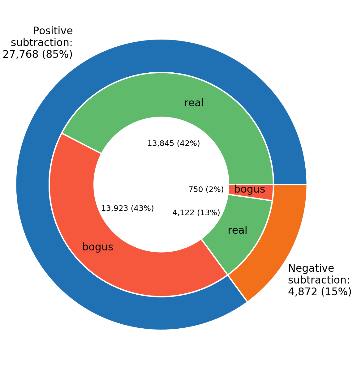
(c) Positive/negative subtraction

Figure 6: Training data breakdown by filters, position in/out of the Galactic plane, and positive/negative subtraction. Percentages of the total are given. As of June 2019, the total number of training examples is 32,640.

2.2 braai architecture and training

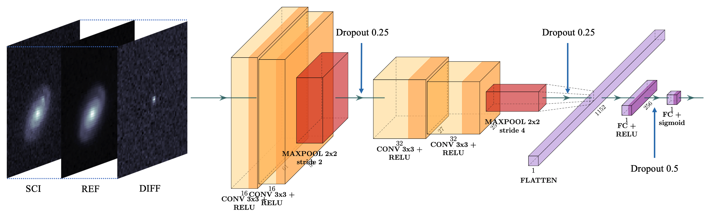
Figure 7: Architecture of the custom VGG6 model. The $L^{2}$-normalized epochal science, reference, and difference cutout images are stacked to form 63x63x3 triplets that are input into the model. ReLU activation functions are used for all five hidden trainable layers; a sigmoid activation function is used for the output layer that produces a score from 0.0 to 1.0. Dropout is used for regularization. See Section 2.2 for the details.

We use a simple custom VGG-like sequential model (“VGG6”) (Simonyan & Zisserman, 2014) (see Fig. 7 for details). The model has six layers with trainable parameters: four convolutional and two fully-connected. The first two convolutional layers use 16 3x3 pixel filters each while in the second pair, 32 3x3 pixel filters are used. To prevent over-fitting, a dropout rate of 0.25 is applied after each max-pooling layer and a dropout rate of 0.5 is applied after the second fully-connected layer. ReLU activation functions are used for all five hidden trainable layers; a sigmoid activation function is used for the output layer.

We also implemented more complicated architectures such as 18- and 50-layer deep models based on residual connections (“ResNet18” and “ResNet50”), but observed no performance gain and therefore only use the VGG6 model.

The cutout images that are generated by the ZSDS are centered on the event candidate and are of size 63x63 pixels (or smaller, if the event is detected near the CCD edge) at a plate scale of $1\arcsec$ per pixel. We perform independent $L^{2}$-normalization of the epochal science, reference, and difference cutouts and stack them to form 63x63x3 triplets that are input into the model. Smaller examples are accordingly padded using a constant pixel value of $10^{-9}$.

Braai is implemented using TensorFlow software and its high-level Keras API (Abadi et al., 2015; Chollet et al., 2015). We used the binary cross-entropy loss function, the Adam optimizer (Kingma & Ba, 2014), a batch size of 64, and a 81%/9%/10% training/validation/test data split. The training image data were weighted per class to mitigate the slight real vs. bogus imbalance in the data sets. The images may be flipped horizontally and/or vertically at random. No random rotations and translations were added.

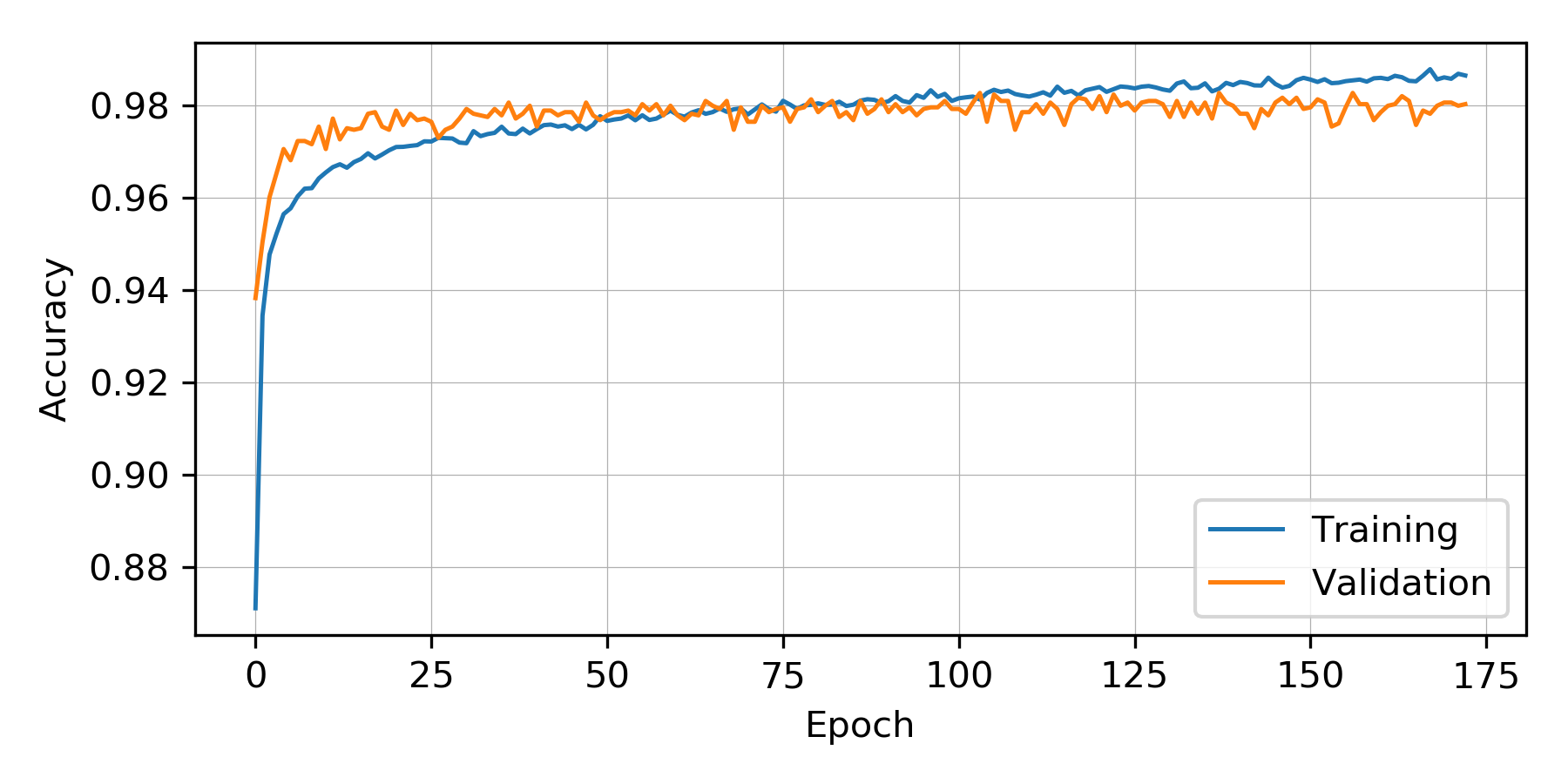
Figure 8: Training (in blue) and validation (in orange) accuracy of braai version $d6\_m7$ that is deployed in production as of June 2019.

We used the early stopping technique to finish training if no improvement in validation accuracy was observed over many epochs. As a result, the model is typically trained for 150-200 epochs. For training, we used an on-premises Nvidia Tesla P100 12G GPU. Training for 200 epochs on $\sim 30k$ images takes about 20 minutes for the VGG6 architecture.

Figure 8 shows training (in blue) and validation (in orange) accuracy for the model version $d6\_m7$ that is deployed in production as of June 2019. Both the training and validation accuracy is about 98%.

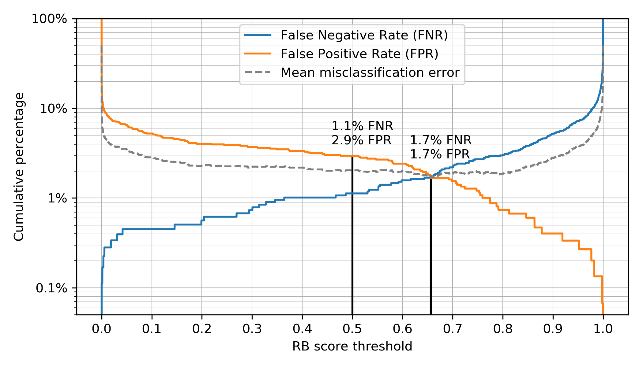
Figure 9: FNR and FPR as functions of the RB score threshold. At a score threshold of 0.5, braai yields $1.1\%$ FNR and $2.9\%$ FPR. At a score threshold of 0.65, braai yields a value of $1.7\%$ for both FNR and FPR. Braai version $d6\_m7$ (deployed in production as of June 2019) was evaluated on 3,271 test examples from the data set.

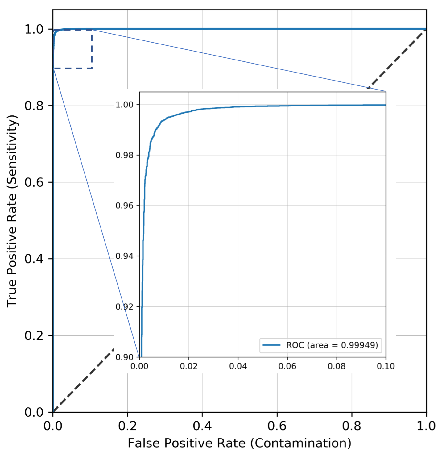
Figure 10: ROC curve of braai version $d6\_m7$ that is deployed in production as of June 2019.

The test performance of the resulting classifier quantified by the false negative rate (FNR) and false positive rate (FPR) as functions of the score threshold is shown in Fig. 9. Fig. 10 displays the receiver operating characteristic (ROC) curve. At a score threshold of 0.5, braai yields $1.1\%$ FNR on the test set (which contained 3,271 examples) while keeping the FPR below $3\%$, as demonstrated in the confusion matrices (Fig. 11). At a score threshold of 0.65, braai yields a value of $1.7\%$ for both FNR and FPR.

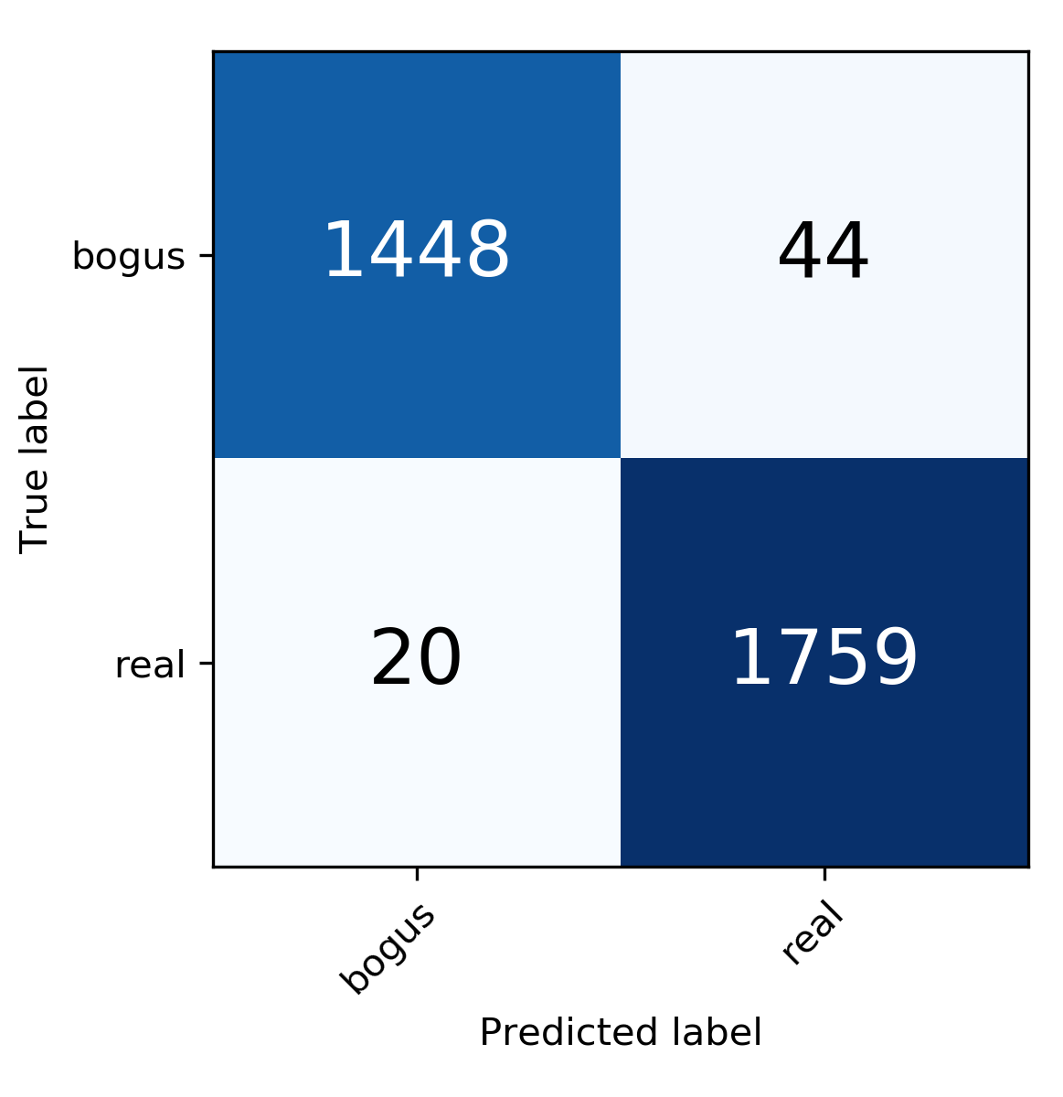
(a) Without normalization

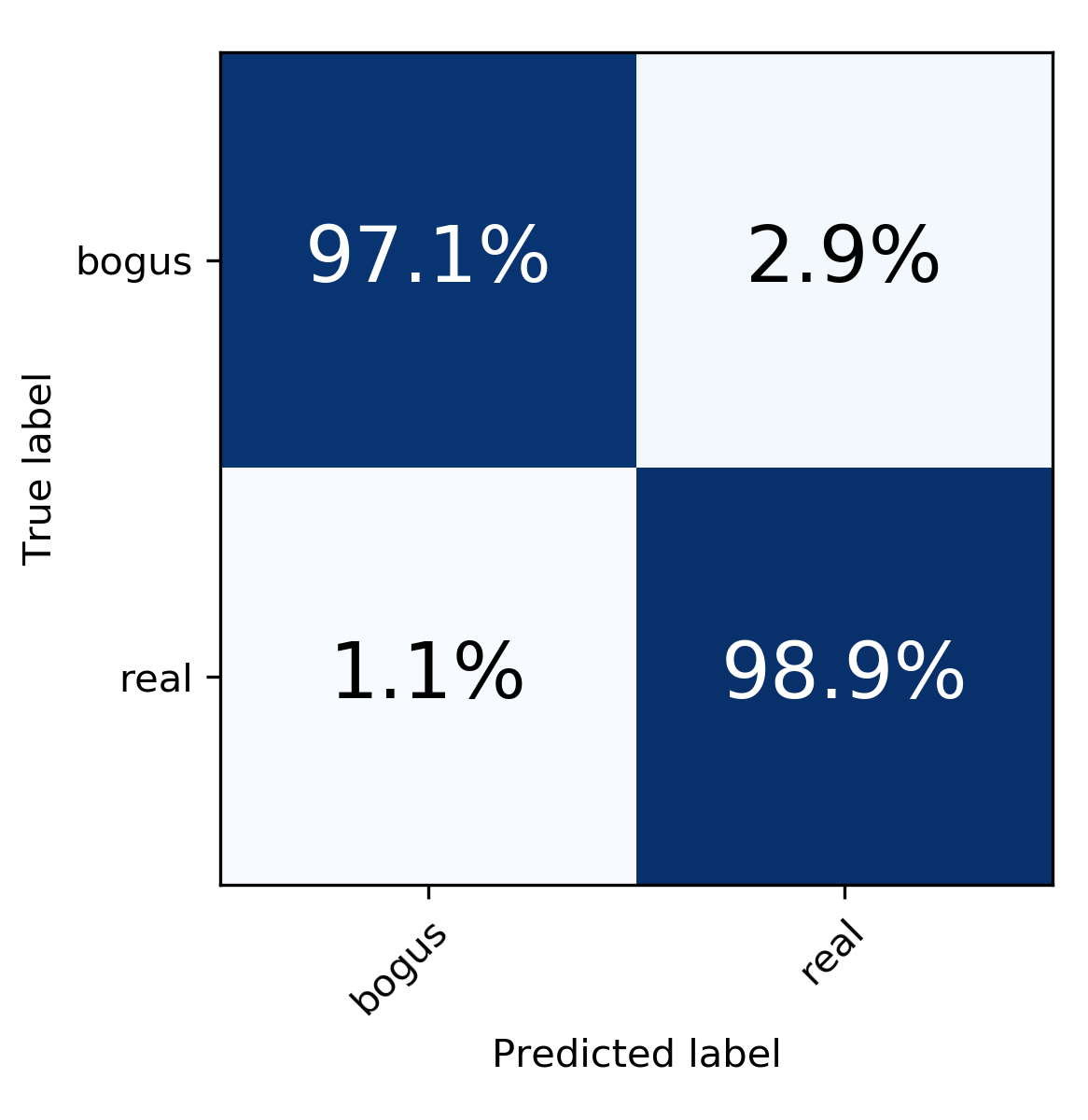
(b) Normalized

Figure 11: Confusion matrices for an RB score threshold of 0.5 for braai version $d6\_m7$ that is deployed in production as of June 2019.

3 Classifier performance

3.1 Zooniverse test set

Zwicky’s Quirky Transients is a Zooniverse project for volunteers to publicly label a set of ZTF candidates as real or bogus (with a skip option). We show only three images per candidate viz. Sci, Ref, and Diff. from which the volunteers are expected to tell apart the two types. One thing we wanted to see was the consensus especially where RF RB scores were ambiguous. Up to ten volunteers could classify the same object. The volunteers were trained through tutorials, a field guide, and by feedback from researchers in interactive Q&A threads. The RF RB score ranges were hand-crafted for them to show examples that were definitely bogus, definitely real, and ambiguous (majority).

Seven campaigns were run between January and May of 2019 involving $\sim 13000$ objects. The first campaign was the largest with 6600 triplets with the following RF $rb$ distribution: $10\%\>rb<.3$, $10\%\>rb>.7$, $80\%\>0.3<=rb<=0.65$. The second and third campaigns had similar $rb$ distributions, and $\sim 1000$ objects each. The last four campaigns also had $\sim 1000$ objects each, but all had $rb>0.4$. For all the campaigns we had excluded objects within 8” of known Solar System objects, and also those that have been found through subtracting the Sci image from the Ref image (i.e. with a fainter Sci image detection compared to the Ref image detection). At the end of the first campaign, we selected a data set consisting of triplets with at least six separate classifications. For this set of 6436, we plotted the $rb$ score against the fraction of real classifications, and selected two areas from the plot – (a) “gold real”: those with $rb$ score $>=0.57$ and classified by at least $70\%$ volunteers as real, and (b) “gold bogus”: those with $rb$ score $<=0.45$ and classified by fewer than $45\%$ volunteers as real. This resulted in the gold real set having 416 triplets and, the gold bogus having 1,196 triplets, for a total of 1612 triplets. These data were then inspected using Zwickyverse and the ZAL and re-labeled if necessary. We found that the real event sample was almost uncontaminated (under 5% FPR), however about 30% of what was labeled as bogus (and also had low RF RB scores) turned out to be real (mainly, variable stars imaged under challenging conditions, something the volunteers could not have known because they had no access to the light curves).

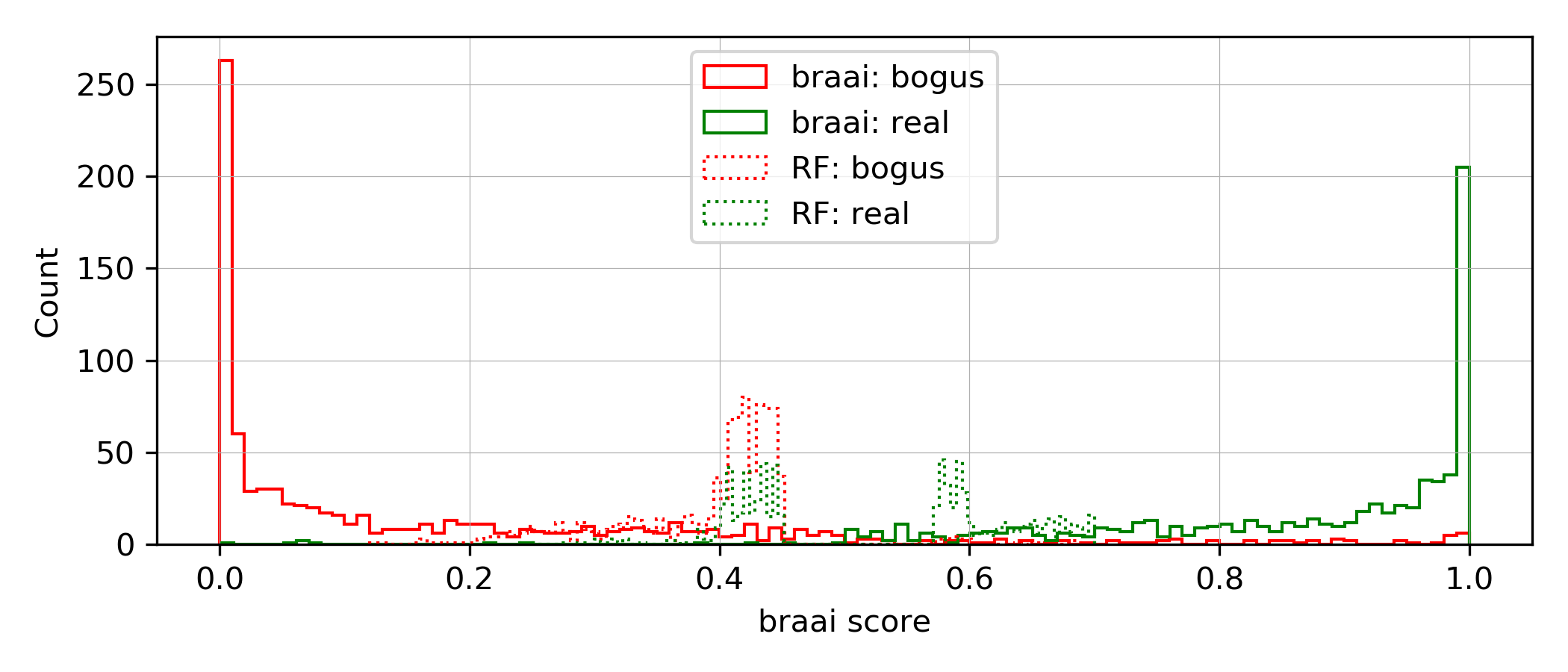
Figure 12: Histogram of braai and RF RB scores for 734 real and 878 bogus examples from the Zooniverse test set. Braai version $d6\_m7$ that is deployed in production as of June 2019. RF RB scores come from multiple versions of the classifier.

Fig. 12 shows the histogram of braai (version $d6\_m7$ deployed in production as of June 2019) and RF RB scores (that come from multiple versions of the classifier) for 734 real and 878 bogus examples from the Zooniverse test set. Evidently, braai yields much more reliable results than the RF classifier. The two peaks around RF RB of 0.5 are a selection effect caused by the input ranges of RB scores chosen for the Zooniverse campaigns.

3.2 Real events

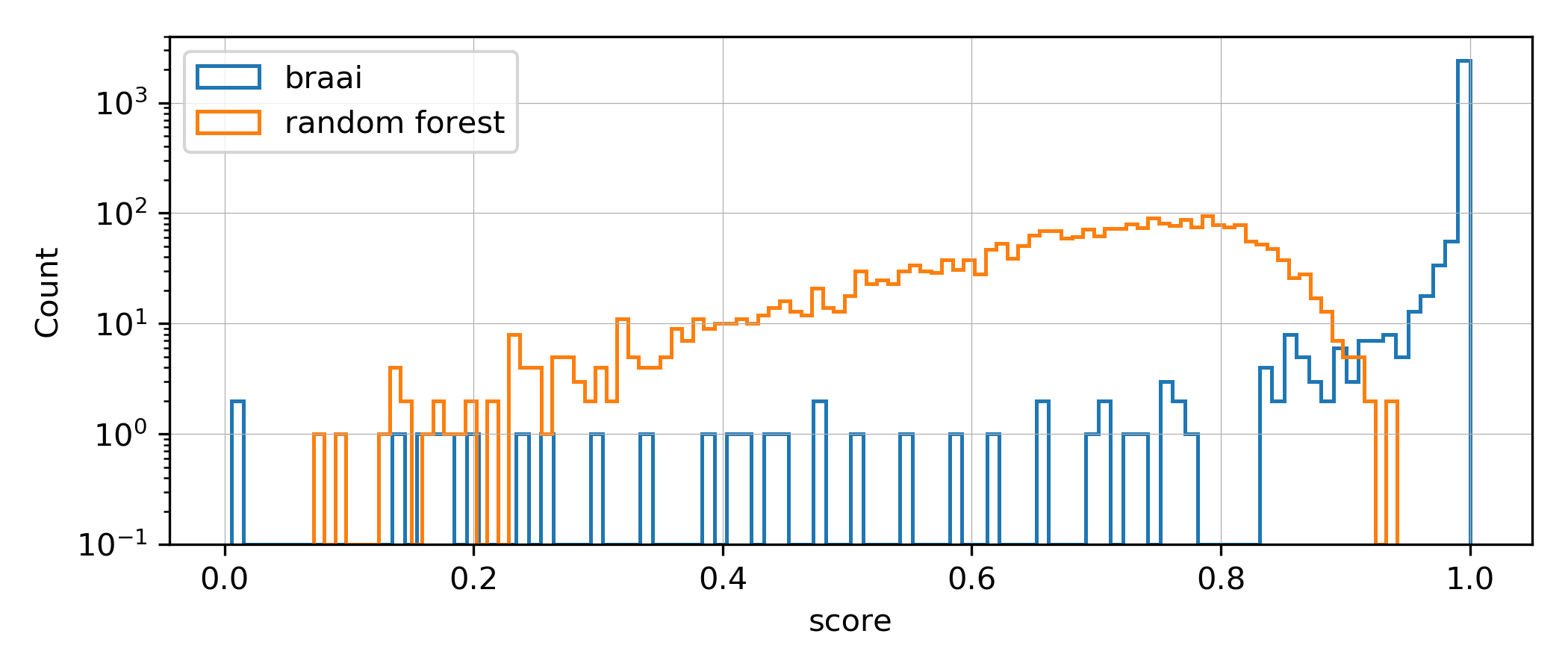
Figure 13: Histogram of braai and RF RB scores of 2,633 ZTF alerts from the night of May 14, 2019 that originated from 921 objects identified as real on the GROWTH marshal. Braai version $d6\_m7$. RF classifier version $t15\_f5\_c3$.

To further test the performance, we evaluated braai on 2,633 ZTF alerts from the night of May 14, 2019 that originated from 921 objects vetted as real by humans on the GROWTH marshal after passing programmatic filters of different science groups (a mix of flux-transient and reoccurring flux-variable objects). Again adopting a score threshold of 0.5, only 18 out of 2633 candidates are misclassified (0.7% FNR) by braai compared to 282 (10.7% FNR) misclassified by the RF classifier deployed at the time. The histogram of braai and RF RB scores is shown in Fig. 13 in logarithmic scale, since the vast majority of these candidates are scored close to unity by braai.

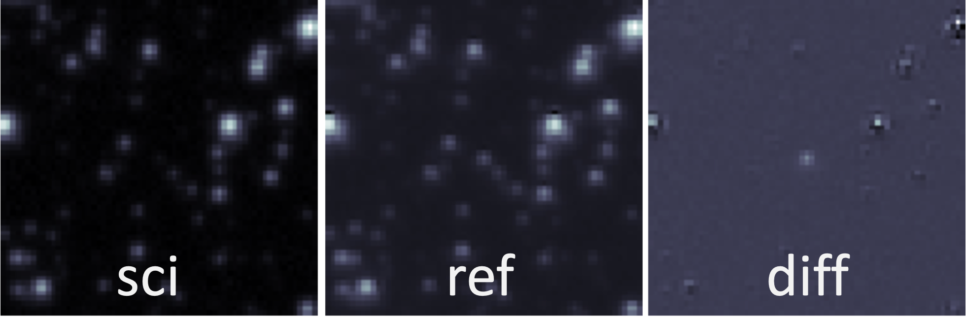
Figure 14: Example 63x63 pixel image triplet (science, reference, difference) from a known reoccurring flux-variable object located in a densely populated region of the sky. ZTF plate scale is $1\arcsec$ per pixel.

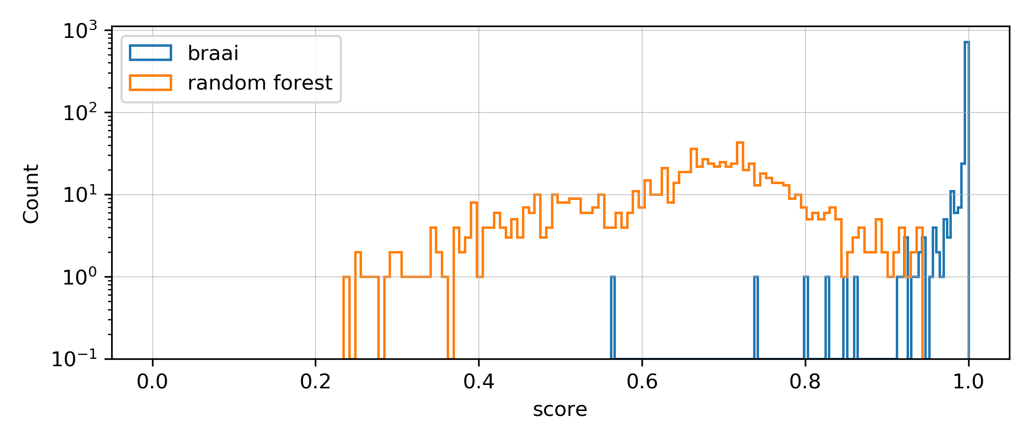
Figure 15: Histogram of braai and RF RB scores of 803 ZTF alerts that originated from objects located in densely populated regions of the sky. Braai version $d6\_m7$ deployed in production as of June 2019. RF RB scores come from multiple versions of the classifier.

Next, we tested the braai performance on 803 alerts from known reoccurring flux-variable objects located in densely populated regions of the sky (see an example triplet on Fig. 14). The alerts were generated from observations covering a wide range of conditions over the course of ZTF’s first year of operation. With a score threshold of 0.5, all candidates are classified correctly by braai compared to 113 misclassifications (14.1% FNR) by the RF classifier. The histogram of braai and RF RB scores is shown in Fig. 15 in logarithmic scale.

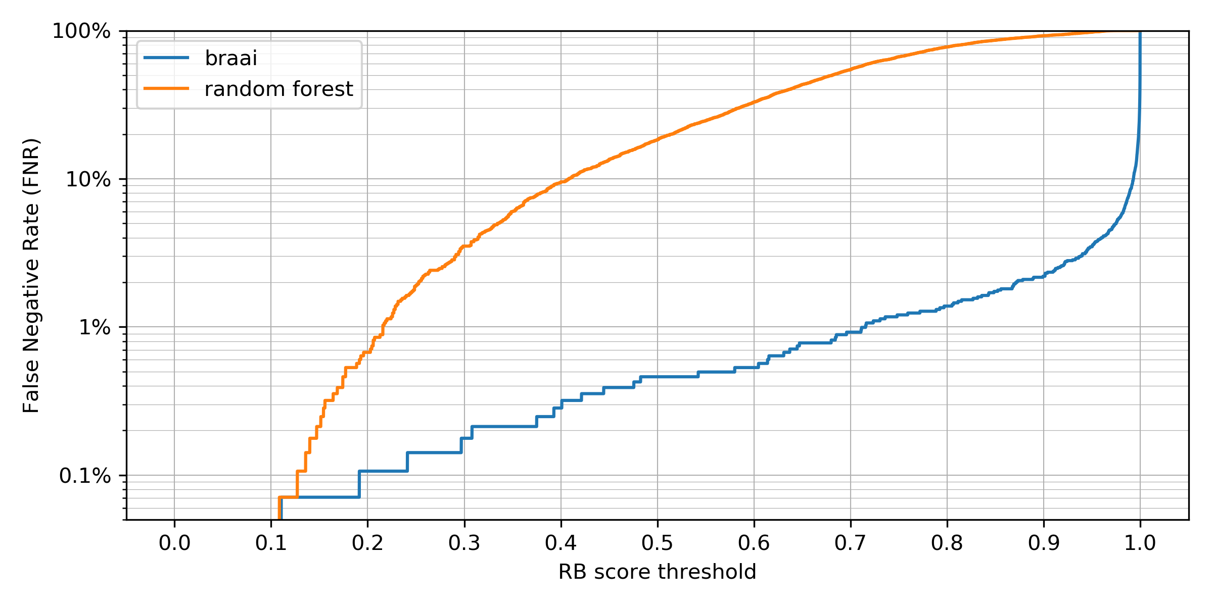
Figure 16: False negative rates of braai and RF RB classifier for 2,820 alerts from a set of 140 supernovae detected by ZTF in 2019. At a score threshold of 0.5, braai correctly identified 99.5% of the SN vs. 80% by RF RB. Braai version $d6\_m7$ deployed in production as of June 2019. RF classifier version $t15\_f5\_c3$ or more recent.

Further, we evaluated braai on 2,820 alerts from a set of 140 recent (detected in 2019) supernovae (SNs). We selected those SNs such that no alerts originating from them were in the training set. As shown in Fig. 16, the FNR of braai stays below 1% up to a score threshold of 0.7 essentially ensuring detection of (even very young) SNs while keeping the FPR below 2% (see Fig. 9), significantly reducing the amount of time spent on SN candidate vetting.

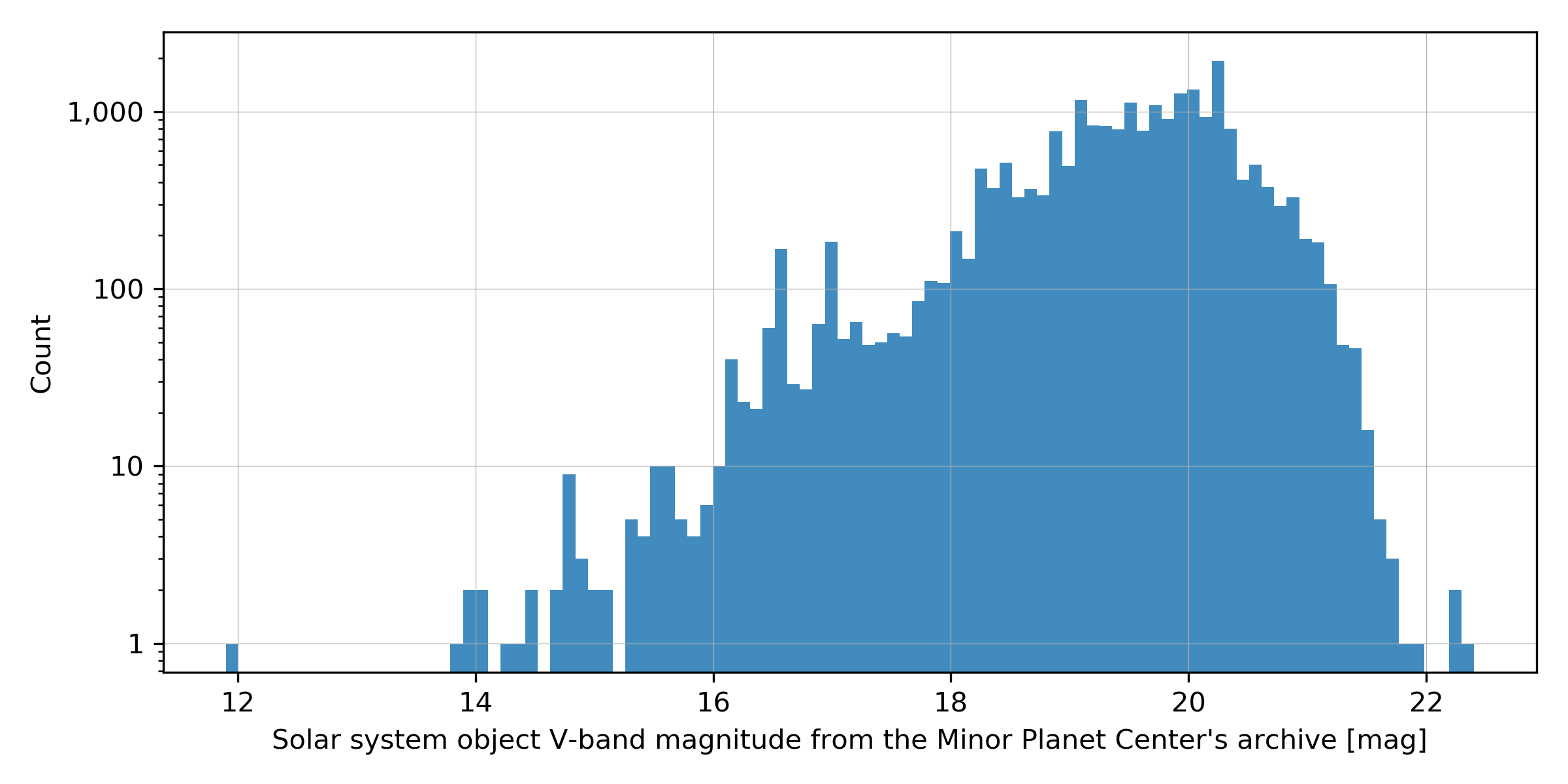
(a) Histogram of Solar system object V-band magnitudes in the set, as reported by the Minor Planet Center archive. The objects are identified automatically, resulting in a set that is not limited to high signal-to-noise levels that humans usually find easy to detect.

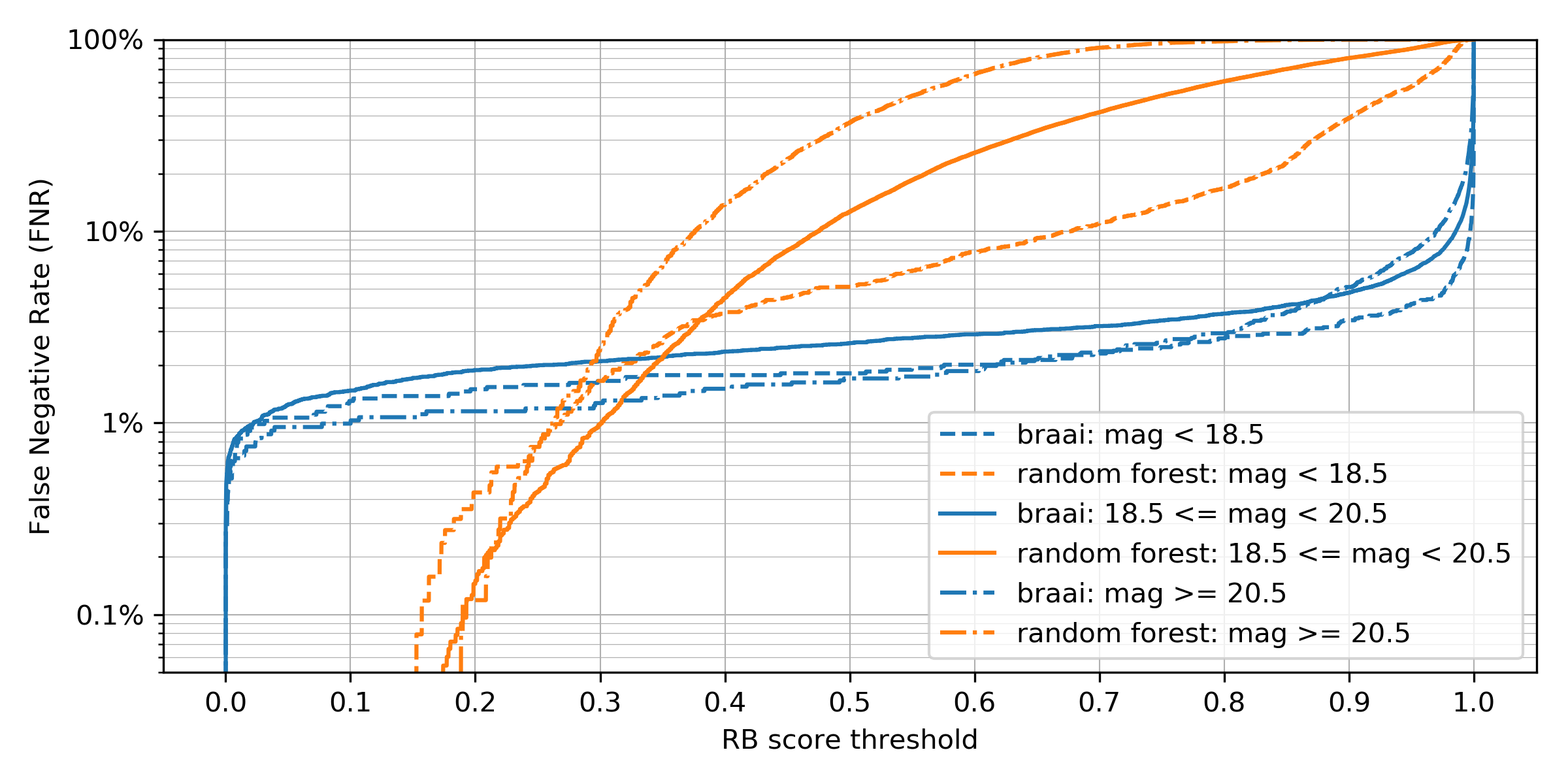
(b) False negative rates of braai vs. RF RB classifier for asteroids with $Vmag<18.5$ (2,534 alerts), $18.5<=Vmag<20.5$ (16,587 alerts), and $Vmag>=20.5$ (2,520 alerts). At a score threshold of 0.5, braai’s FNR stays below 3% regardless of the candidate brightness while for the RF RB classifier the FNR significantly degrades for fainter objects (from $\sim 5\%$ to $\sim 40\%$). Braai version $d6\_m7$, RF classifier version $t17\_f5\_c3$

Figure 17: Braai performance on a set of 21,641 alerts originating from known Solar system objects observed by ZTF in June 2019.

Finally, we evaluated braai on 21,641 alerts originating from known Solar system objects observed by ZTF in June 2019. Since the candidates here are identified automatically, this set is not limited to high signal-to-noise levels that humans usually find easy to detect (see Fig. 17a). Fig. 17b shows the FNR of braai vs. RF RB classifier for asteroids with $Vmag<18.5$ (2,534 alerts), $18.5<=Vmag<20.5$ (16,587 alerts), and $Vmag>=20.5$ (2,520 alerts). At a score threshold of 0.5, braai’s FNR stays below 3% regardless of the candidate brightness while for the RF RB classifier the FNR significantly degrades for fainter objects (from $\sim 5\%$ to $\sim 40\%$).

3.3 Production deployment and Edge TPUs

Braai was recently integrated into the ZSDS’ image-differencing and event-extraction pipeline, which executes on a compute cluster of 66 commodity dual-socket Intel Xeon servers (Masci et al., 2019). The score and model version (drb and drbversion) are recorded in the candidate block of each alert packet. The braai score is provided "as is" as a reliability metric and is not used to filter the outgoing alert stream. The individual science groups/users use different thresholds depending on the science case and their FNR/FPR requirements.

While, currently, the model, being relatively small in size, is evaluated on CPUs in production, we have experimented with alternative solutions. Concretely, we produced a version of braai that can be executed on Edge TPUs made by Google under the Coral brand – a new class of efficient and cheap ($\sim\$100$) devices designed for heavy ML inference workloads. Currently, Edge TPUs can only operate with quantized models, i.e. both the model input and tensor parameters must be 8-bit fixed-point numbers. To achieve this, we performed quantization-aware training in TensorFlow, which uses “fake” quantization nodes to simulate the effect of 8-bit values during training, thus allowing inference to run using the quantized values. This technique makes the model more tolerant of the lower precision values, which generally results in a higher accuracy model (compared to post-training quantization). The quantized model is subsequently converted to TensorFlow Lite and compiled for Edge TPU usage.

This Edge TPU-native version of braai was deployed on a Raspberry Pi 3 Model B+ single-board computer with a USB Edge TPU accelerator. Although the scores produced by it are scaled 8-bit integers and thus less numerically precise, braai_edgetpu yields virtually the same performance as the full version of braai at a score threshold of 0.5 and it takes about ten minutes to process a typical night of ZTF alerts (200,000). We have also deployed braai_edgetpu on the Edge-TPU-enabled Coral Dev board and were able to achieve a $4-5\times$ faster processing rate of up to 1200 triplets per second.

We stress that even quite complicated DL architectures can be efficiently executed on these devices with minimal effect on the inference accuracy making costly (potentially cloud-based) GPU work flows virtually unnecessary. This has significant implications for current and future surveys.

4 Conclusions

We have demonstrated that by putting together a large, representative, and uncontaminated data set with a relatively simple DL model we can achieve a state-of-the-art real/bogus classification performance. To improve it even further, we will retrain and deploy new classifiers as more labeled data are collected, especially in the $i$-band and at low Galactic latitudes, and if there are changes made to the hardware, or to intermediate readout and processing steps. With more data we may split the classifier for $g$, $r$, and $i$ bands, but the current performance suggests that that may not be required.

We note that the RB score provides only one reliability metric. Different ZTF science groups perform additional filtering using multiple alert columns (see Kasliwal et al. (2019)).

The data set that we put together for this project will be used in future work on DL system currently under development, such as specialized classifiers. It should be easy to reuse/extend this setup for other surveys including the Large Synoptic Survey Telescope (LSST, Ivezić et al. (2008)) in the not far future.

Braai code and pre-trained models are available at https://github.com/dmitryduev/braai

References

- Abadi et al. (2015) Abadi M., et al., 2015, TensorFlow: Large-Scale Machine Learning on Heterogeneous Systems, https://www.tensorflow.org/
- Aldering et al. (2002) Aldering G., et al., 2002, in Tyson J. A., Wolff S., eds, Proc. SPIEVol. 4836, Survey and Other Telescope Technologies and Discoveries. pp 61–72, doi:10.1117/12.458107
- Bailey et al. (2007) Bailey S., Aragon C., Romano R., Thomas R. C., Weaver B. A., Wong D., 2007, ApJ, 665, 1246
- Bellm et al. (2019) Bellm E. C., et al., 2019, Publications of the Astronomical Society of the Pacific, 131, 018002
- Bertin (2010) Bertin E., 2010, SWarp: Resampling and Co-adding FITS Images Together, Astrophysics Source Code Library (ascl:1010.068)
- Bloom et al. (2008) Bloom J., Starr D., Butler N., Nugent P., Rischard M., Eads D., Poznanski D., 2008, Astronomische Nachrichten, 329, 284
- Brink et al. (2012) Brink H., Richards J. W., Poznanski D., Bloom J. S., Rice J., Negahban S., Wainwright M., 2012, arXiv:1209.3775
- Cabrera-Vives et al. (2017) Cabrera-Vives G., Reyes I., Förster F., Estévez P. A., Maureira J.-C., 2017, ApJ, 836, 97
- Chollet et al. (2015) Chollet F., et al., 2015, Keras, https://keras.io
- Dekany & Smith (2019) Dekany R., Smith R., 2019, The Zwicky Transient Facility: Observing System, In prep.
- Drake et al. (2009) Drake A. J., et al., 2009, ApJ, 696, 870
- Goldstein et al. (2015) Goldstein D. A., et al., 2015, AJ, 150, 82
- Graham et al. (2019) Graham M. J., et al., 2019, PASP, 131, 078001
- Ivezić et al. (2008) Ivezić v., et al., 2008
- Kasliwal et al. (2019) Kasliwal M. M., et al., 2019, Publications of the Astronomical Society of the Pacific, 131, 038003
- Kingma & Ba (2014) Kingma D. P., Ba J., 2014, arXiv e-prints, p. arXiv:1412.6980
- Law et al. (2009) Law N. M., et al., 2009, PASP, 121, 1395
- Mahabal et al. (2019) Mahabal A., et al., 2019, PASP, 131, 038002
- Masci et al. (2019) Masci F. J., et al., 2019, Publications of the Astronomical Society of the Pacific, 131, 018003
- McCulloch & Pitts (1943) McCulloch W. S., Pitts W., 1943, The bulletin of mathematical biophysics, 5, 115
- Rebbapragada et al. (2015) Rebbapragada U., Bue B., Wozniak P. R., 2015. p. 434.02, http://adsabs.harvard.edu/abs/2015AAS...22543402R
- Reyes et al. (2018) Reyes E., Estévez P. A., Reyes I., Cabrera-Vives G., Huijse P., Carrasco-Davis R., Förster F., 2018, arXiv e-prints, p. arXiv:1808.03626
- Simonyan & Zisserman (2014) Simonyan K., Zisserman A., 2014, arXiv e-prints, p. arXiv:1409.1556
- Wozniak et al. (2013) Wozniak P. R., Moody D. I., Ji Z., Brumby S. P., Brink H., Richards J., Bloom J. S., 2013. p. 431.05, http://adsabs.harvard.edu/abs/2013AAS...22143105W
- Wright et al. (2015) Wright D. E., et al., 2015, MNRAS, 449, 451
- Zackay et al. (2016) Zackay B., Ofek E. O., Gal-Yam A., 2016, ApJ, 830, 27