A renormalized approach to
neutrinoless double-beta decay

Abstract

The process at the heart of neutrinoless double-beta decay, $nn\rightarrow pp\,e^{-}e^{-}$ induced by a light Majorana neutrino, is investigated in pionless and chiral effective field theory. We show in various regularization schemes the need to introduce a short-range lepton-number-violating operator at leading order, confirming earlier findings. We demonstrate that such a short-range operator is only needed in spin-singlet $S$-wave transitions, while leading-order transitions involving higher partial waves depend solely on long-range currents. Calculations are extended to include next-to-leading corrections in perturbation theory, where to this order no additional undetermined parameters appear. We establish a connection based on chiral symmetry between neutrinoless double-beta decay and nuclear charge-independence breaking induced by electromagnetism. Data on the latter confirm the need for a leading-order short-range operator, but do not allow for a full determination of the corresponding lepton-number-violating coupling. Using a crude estimate of this coupling, we perform ab initio calculations of the matrix elements for neutrinoless double-beta decay for ⁶He and ¹²Be. We speculate on the phenomenological impact of the leading short-range operator on the basis of these results.

I Introduction

The observation of neutrino oscillations has demonstrated that neutrinos are massive particles, with masses constrained by single-beta ($\beta$) decay experiments Aseev et al. (2011) and cosmological observations Akrami et al. (2018) to be several orders of magnitude smaller than those of the charged leptons. The smallness of the neutrino masses suggests that they have a different origin with respect to other Standard Model (SM) particles. In particular, neutrinos, the only fundamental charge-neutral fermions in the SM, could have a Majorana mass, whose small value naturally arises in the “see-saw” mechanism Minkowski (1977); Mohapatra and Senjanovic (1980); Gell-Mann et al. (1979). A distinctive signature of the Majorana nature of neutrino masses is the violation of lepton number ($L$) by two units ($|\Delta L|=2$) Schechter and Valle (1982), which would manifest itself in processes such as neutrinoless double-beta decay ($0\nu\beta\beta$), nuclear muon-to-positron conversion, or rare meson decays such as $K^{+}\rightarrow\pi^{-}e^{+}e^{+}$. $0\nu\beta\beta$ Haxton and Stephenson (1984) is by far the most sensitive laboratory probe of lepton number violation (LNV). Current experimental limits are very stringent Gando et al. (2013); Agostini et al. (2013); Albert et al. (2014); Andringa et al. (2016); Gando et al. (2016); Elliott et al. (2016); Agostini et al. (2017); Aalseth et al. (2018); Albert et al. (2018); Alduino et al. (2018); Agostini et al. (2018); Azzolini et al. (2018); Anton et al. (2019), e.g. $T^{0\nu}_{1/2}>1.07\times 10^{26}$ yr for ¹³⁶Xe Gando et al. (2016), with the next-generation ton-scale experiments aiming for improvements by one or two orders of magnitude.

The interpretation of $0\nu\beta\beta$ experiments and the constraints on fundamental LNV parameters, such as the Majorana masses of left-handed neutrinos, rely on having a general theoretical framework that provides reliable predictions with controlled uncertainties. Contributions to $0\nu\beta\beta$ can be organized in terms of $SU(3)_{\rm c}\times U(1)_{\rm em}$-invariant operators Prezeau et al. (2003); Graesser (2017); Cirigliano et al. (2017, 2018a) at the scale $\Lambda_{\chi}\sim 1$ GeV characteristic of QCD nonperturbative effects. The operator of lowest dimension is a Majorana mass term for light, left-handed neutrinos,

$$\mathcal{L}_{|\Delta L|=2}=-\frac{m_{\beta\beta}}{2}\,\nu_{eL}^{T}C\,\nu_{eL}+\ldots,$$ (1)

where $C=i\gamma_{2}\gamma_{0}$ denotes the charge conjugation matrix and the effective neutrino mass $m_{\beta\beta}=\sum U_{ei}^{2}m_{i}$ combines the neutrino masses $m_{i}$ and the elements $U_{ei}$ of the Pontecorvo-Maki-Nakagawa-Sato (PMNS) matrix. Because of the $SU(2)_{L}$ invariance of the SM, $m_{i}\sim v^{2}/\Lambda$, where $v\simeq 246$ GeV is the vacuum expectation value of the Higgs field and $\Lambda$ is the high-energy scale at which LNV arises Weinberg (1979a). The dots in Eq. (1) denote higher-dimensional LNV operators, which are suppressed by more powers of $v/\Lambda$ and $\Lambda_{\chi}/v$ Cirigliano et al. (2018a).

In this paper we focus on the $0\nu\beta\beta$ transition operator induced by $m_{\beta\beta}$. The quark-level Lagrangian we consider is given by

$${\cal L}_{\rm eff}={\cal L}_{\rm QCD}-\frac{4G_{F}}{\sqrt{2}}V_{ud}\,\bar{u}_{L}\gamma^{\mu}d_{L}\,\bar{e}_{L}\gamma_{\mu}\nu_{eL}-\frac{m_{\beta\beta}}{2}\,{\nu}_{eL}^{T}C\nu_{eL}+{\rm H.c.},$$ (2)

where the first term denotes the strong interactions among quarks and gluons, and the second term represents the weak interactions of up and down quarks and leptons, whose strength is determined by the Fermi constant $G_{F}$ and the $V_{ud}$ element of the Cabibbo-Kobayashi-Maskawa (CKM) matrix. In order to calculate $0\nu\beta\beta$ transitions, the Lagrangian in Eq. (2) needs to be matched onto a theory of hadrons,

$$\mathcal{L} = \mathcal{L}_{\rm strong}(\pi,N,\Delta)-\frac{4G_{F}}{\sqrt{2}}V_{ud}\,\mathcal{J}_{\mu}(\pi,N,\Delta)\,\bar{e}_{L}\gamma^{\mu}\nu_{eL}$$ (3)

$$-\frac{1}{2}m_{\beta\beta}\,{\nu}_{eL}^{T}C\nu_{eL}-\frac{4G_{F}}{\sqrt{2}}V_{ud}\,\mathcal{O}(\pi,N,\Delta)\,\bar{e}\,\Gamma C\bar{\nu}_{eL}^{T}-G_{F}^{2}\,\mathcal{O}^{\prime}(\pi,N,\Delta)\,\bar{e}\,\Gamma C\bar{e}+\textrm{H.c.},$$

where again the first and second terms represent the strong and weak interactions, respectively, while the operators in the second line violate $L$ by two units. Here $\mathcal{L}_{\rm strong}$, $\mathcal{J}_{\mu}$, $\mathcal{O}$, and $\mathcal{O}^{\prime}$ are combinations of pion, nucleon, and Delta isobar fields. $\Gamma$ represents the possible Dirac structures of the leptonic bilinear, and we are suppressing, for simplicity, possible Lorentz indices on $\Gamma$, $\mathcal{O}$, and $\mathcal{O}^{\prime}$. For the short-range operators induced by light Majorana-neutrino exchange, $\Gamma=1$. For low-energy hadronic and nuclear processes, Eq. (3) can be organized using chiral effective field theory ($\chi$EFT) Weinberg (1979b, 1990, 1991) according to the scaling of operators in powers of the typical momentum in units of the breakdown scale,

$$\epsilon_{\chi}=Q/\Lambda_{\chi}~{},\qquad Q\sim m_{\pi},\qquad\Lambda_{\chi}\sim 4\pi F_{\pi},$$ (4)

where $m_{\pi}\simeq 140$ MeV and $F_{\pi}\simeq 92.2$ MeV are the pion mass and decay constant, respectively. Given that the quark-level Lagrangian breaks $L$, all possible $|\Delta L|=2$ operators are generated at some order in $G_{F}$ and $\epsilon_{\chi}$.

The Lagrangian in Eq. (3) can then be used to derive the $0\nu\beta\beta$ transition operator, often referred to as the “neutrino potential”. A leading contribution to the transition operator is induced by the exchange of neutrinos between two nucleons, mediated by the single-nucleon vector and axial currents. Defining the effective Hamiltonian as

$$H_{\rm eff}=H_{\rm strong}+2G_{F}^{2}V_{ud}^{2}\,m_{\beta\beta}\,\bar{e}_{L}C\bar{e}_{L}^{T}\,\sum_{a\neq b}V^{(a,b)}_{\nu}\,,$$ (5)

the long- and pion-range contributions to the neutrino potential between two nucleons labeled 1 and 2 are given, at leading order (LO), by

$$V^{(1,2)}_{\nu\,\rm L}=\frac{\tau^{(1)+}\tau^{(2)+}}{{\mathbf{q}}^{2}}\left[1-\frac{2g_{A}^{2}}{3}\mbox{\boldmath$\sigma$}^{(1)}\cdot\mbox{\boldmath$\sigma$}^{(2)}\left(1+\frac{m_{\pi}^{4}}{2({\mathbf{q}}^{2}+m_{\pi}^{2})^{2}}\right)-\frac{g_{A}^{2}}{3}S^{(12)}\left(1-\frac{m_{\pi}^{4}}{({\mathbf{q}}^{2}+m_{\pi}^{2})^{2}}\right)\right],$$ (6)

where $g_{A}=1.27$ is the nucleon axial coupling, ${\mathbf{q}}$ is the transferred momentum, $\tau^{+}$ is the isospin-raising Pauli matrix, $\sigma$ are the Pauli spin matrices, and $S^{(12)}=\mbox{\boldmath$\sigma$}^{(1)}\cdot\mbox{\boldmath$\sigma$}^{(2)}-3\mbox{\boldmath$\sigma$}^{(1)}\cdot{\mathbf{q}}\,\mbox{\boldmath$\sigma$}^{(2)}\cdot{\mathbf{q}}/{\mathbf{q}}^{2}$ is the spin tensor operator. We use the subscript L to indicate that Eq. (6) is a long-range potential. In the rest of the paper, we will drop the nucleon labels in $V_{\nu}$. Corrections from the momentum dependence of the nucleon vector and axial form factors, as well as from weak magnetism, are usually included in the neutrino potential, see for example Ref. Engel and Menéndez (2017); Ejiri et al. (2019). These corrections contribute at next-to-next-to-leading order (N²LO) in $\chi$EFT. At this order, there appear many other contributions, for instance from pion loops that dress the neutrino exchange and from processes involving new hadronic interactions with the associated parameters, or “low-energy constants” (LECs) Cirigliano et al. (2018b).

The $0\nu\beta\beta$ transition operator in Eq. (6) has a Coulomb-like behavior at large $|{\mathbf{q}}|$, which induces ultraviolet (UV) divergences in LNV scattering amplitudes, such as $nn\rightarrow pp\,e^{-}e^{-}$ , when both the two neutrons in the initial state and the two protons in the final state are in the ${}^{1}S_{0}$ channel. Our main goal in this work is to investigate these divergences and their consequence: the need for a new short-range $0\nu\beta\beta$ operator at LO Cirigliano et al. (2018c). This situation is analogous to charge-independence breaking (CIB) in nucleon-nucleon ($N\!N$) scattering, which receives long-range contributions from Coulomb-photon exchange and from the pion-mass splitting in pion exchange. The consistency of the EFT requires then that, in addition to these long-range contributions, one should include also short-range CIB $N\!N$ operators. This observation is consistent with fits to $N\!N$ scattering data, which, for both chiral potentials Machleidt and Entem (2011); Piarulli et al. (2015); Epelbaum et al. (2015); Ekström et al. (2015); Piarulli et al. (2016); Reinert et al. (2018) and phenomenological potentials such as Argonne $v_{18}$ Wiringa et al. (1995) and CD-Bonn Machleidt (2001), require sizable short-range CIB. A short-range $0\nu\beta\beta$ operator also appears at LO Cirigliano et al. (2018b) in a simpler EFT, pionless EFT (${/\pi}$EFT), where all hadronic degrees of freedom other than the nucleon are integrated out.

In this paper we build upon Refs. Cirigliano et al. (2018b, c) and study the $0\nu\beta\beta$ transition operator up to next-to-leading order (NLO) in $\chi$EFT. We begin in Sec. II by illustrating the problem of having just a long-range neutrino-exchange transition operator at LO, without going into any technical detail. The lepton-number-violating operators in the two EFTs, pionless EFT and chiral EFT, are constructed in Sec. III. (Operators with multiple quark-mass insertions are relegated to App. A.) In Sec. IV we study the scattering amplitude $nn\rightarrow pp\,e^{-}e^{-}$ at LO, using different regulators and renormalization schemes. (Details about the $\overline{\rm MS}$ scheme are given in App. B.) In all schemes, and independently of the inclusion of pions as dynamical degrees of freedom, the matrix element of the neutrino potential $V_{\nu\,\rm L}$ between $N\!N$ wavefunctions in the ${}^{1}S_{0}$ state shows logarithmic sensitivity to short-distance physics, which is cured by including an LO LNV counterterm. In Sec. V we study the transition operator in higher partial waves, such as ${}^{3}P_{J}$ and ${}^{1}D_{2}$. Weinberg’s original power counting Weinberg (1990, 1991) leads to inconsistencies for $N\!N$ interactions in certain spin-triplet waves such as ${}^{3}P_{0}$ Nogga et al. (2005); Pavón Valderrama and Ruiz Arriola (2006), which require the promotion of contact operators to LO in these waves. Yet, we show that, after the strong interaction is properly renormalized, LNV matrix elements are well defined, and do not require further renormalization. In Sec. VI we extend the analysis beyond LO. We consider only the ${}^{1}S_{0}$ channel, which receives a new contribution from strong interactions at NLO Long and Yang (2012). We again study the two EFTs, and show that no additional independent LNV counterterms are needed at this order. In Sec. VII we discuss the relation between $0\nu\beta\beta$ and CIB in $N\!N$ scattering and argue that scattering data show evidence for a CIB contact interaction in the ${}^{1}S_{0}$ channel at LO in $\mathcal{O}(e^{2})$, where $e$ is the proton charge. While chiral and isospin symmetry allow us to derive relations between the CIB and LNV contact interactions, we show that unfortunately scattering data are not enough to unambiguously determine the latter. In Sec. VIII we explore the implications of the LO short-range contribution to the neutrino potential on the $0\nu\beta\beta$ nuclear matrix elements in light nuclei, whose wavefunctions can be computed ab initio, and we conclude in Sec. IX.

II The problems of the leading-order neutrino potential

The main theoretical problem is to connect the Majorana mass term in Eq. (1) to the experimental $0\nu\beta\beta$ rate for various nuclear isotopes. Traditionally, this connection is made by considering the exchange of a neutrino between two neutrons in a nucleus. An insertion of the neutrino Majorana mass on the neutrino propagator is required to account for the violation of lepton number by two units. At tree level, the process $nn\rightarrow pp\,e^{-}e^{-}$ can happen either via a direct neutrino exchange between neutrons or via intermediate pions which then decay into a neutrino and electron. The relevant diagrams are shown in Fig. 1 and lead to the so-called neutrino transition operator or neutrino potential in Eq. (6).

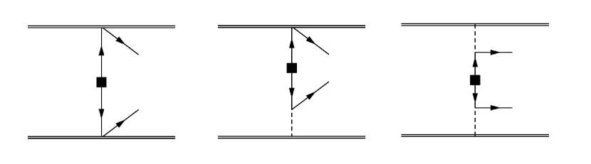
Figure 1: Long-range contributions to the neutrino potential. Double and dashed lines denote, respectively, nucleons and pions. Single lines denote electrons and neutrinos, and a square an insertion of $m_{\beta\beta}$.

To obtain the $0\nu\beta\beta$ nuclear matrix element this transition operator is inserted between all pairs of neutrons in a nucleus using advanced nuclear many-body methods Engel and Menéndez (2017). Typically such calculations apply a closure approximation to take into account the effects of intermediate nuclear excited states, effectively shifting ${\mathbf{q}}^{-2}\rightarrow|{\mathbf{q}}|^{-1}(|{\mathbf{q}}|+\bar{E})^{-1}$ in terms of the closure energy $\bar{E}=\mathcal{O}(\textrm{MeV})$. Such corrections can be shown to occur at higher order if the neutrino transition operator is derived with the $\chi$EFT power-counting rules Cirigliano et al. (2018b). We will not consider it here and set $\bar{E}=0$ for simplicity. Our concerns in this section involve large values of $|{\mathbf{q}}|$ and therefore are not affected by the closure approximation.

For a theoretical study of the neutrino transition operator it is convenient to perform a Gedanken experiment involving two neutrons in the ${}^{1}S_{0}$ state, the simplest nuclear system where the operator can act. Higher partial waves will be studied in a later section. The transition operator can be straightforwardly projected onto the ${}^{1}S_{0}\rightarrow{}^{1}S_{0}$ channel, where it takes a simpler form

$$V_{\nu\,\rm L}^{{}^{1}S_{0}}({\mathbf{q}})=\frac{\tau^{(1)+}\tau^{(2)+}}{{\mathbf{q}}^{2}}\left[1+2g_{A}^{2}+\frac{g_{A}^{2}m_{\pi}^{4}}{({\mathbf{q}}^{2}+m_{\pi}^{2})^{2}}\right]\,.$$ (7)

The transition operator is clearly Coulomb-like, scaling as ${\mathbf{q}}^{-2}$, and therefore typically expected to drop off sufficiently fast for large $|{\mathbf{q}}|$ (or short distances $|{\mathbf{r}}|$) to give rise to finite nuclear matrix elements. As we demonstrate in this section, and study in significant detail below, this expectation turns out to be false.

Before going into a more detailed analysis we wish to explicitly demonstrate the problem here. We want to calculate the amplitude 

$$\mathcal{A}_{\nu}(E,E^{\prime})=-\langle\Psi_{pp}(E^{\prime})|V_{\nu\,\rm L}^{{}^{1}S_{0}}|\Psi_{nn}(E)\rangle,$$ (8)

for the process $nn\rightarrow pp\,e^{-}e^{-}$ where both initial $|\Psi_{nn}(E)\rangle$ and final $|\Psi_{pp}(E^{\prime})\rangle$ states are in the ${}^{1}S_{0}$ channel. We denote by $E={\mathbf{p}}^{2}/m_{n}$ and $E^{\prime}={\mathbf{p}}^{\prime 2}/m_{p}$ the center-of-mass energies of the incoming neutrons and outgoing protons of masses $m_{n}$ and $m_{p}$, respectively, and by ${\mathbf{p}}$ and ${\mathbf{p}}^{\prime}$ the corresponding relative momenta. Without loss of generality, in this section we assume the outgoing electrons to be at rest such that

$$E^{\prime}=E+2(m_{n}-m_{p}-m_{e}),\qquad|{\mathbf{p}}^{\prime}|=\sqrt{{\mathbf{p}}^{2}+2m_{N}(m_{n}-m_{p}-m_{e})},$$ (9)

with $m_{e}$ the electron mass and $2m_{N}=m_{n}+m_{p}$. When working at the kinematic point (9), we will drop, for simplicity, the second argument in $\mathcal{A}_{\nu}$.

The initial- and final-state wavefunctions are obtained by solving the Lippmann-Schwinger or Schrödinger equation involving the strong $N\!N$ potential. Of the latter there exist many variants but most include the long-ranged one-pion exchange and short-range pieces, which are described by the exchange of heavier mesons and/or by arbitrary short-range functions (phenomenological potentials), or else by $N\!N$ contact interactions ($\chi$EFT potentials). Our arguments are best illustrated by use of the LO $\chi$EFT potential in the ${}^{1}S_{0}$ channel, which consists of only two terms,

$$V_{N\!N}^{{}^{1}S_{0}}=C+V_{\pi}^{{}^{1}S_{0}}({\mathbf{q}}),$$ (10)

where

$$V_{\pi}^{{}^{1}S_{0}}({\mathbf{q}})=-\frac{g_{A}^{2}}{4F_{\pi}^{2}}\frac{m_{\pi}^{2}}{{\mathbf{q}}^{2}+m_{\pi}^{2}}$$ (11)

is the Yukawa potential written in terms of the transferred momentum ${\mathbf{q}}={\mathbf{p}}-{\mathbf{p}}^{\prime}$, and $C$ is a contact interaction that accounts for short-range physics from pion exchange and other QCD effects. The latter is needed for renormalization and to generate the observed, shallow ${}^{1}S_{0}$ virtual state. It is expected at LO Weinberg (1990, 1991) on the basis of the naive dimensional analysis (NDA) Manohar and Georgi (1984), and discussed in detail in Sec. III.2.

To obtain the $N\!N$ wavefunctions, $V_{N\!N}^{{}^{1}S_{0}}$ must be iterated to all orders, which we do by numerically solving the Lippmann-Schwinger or Schrödinger equation. Because of the short-range pieces in the potential, the involved integrals are in general divergent and require regularization. In this section we will use a coordinate-space cutoff $R_{S}$ but other regulators will be discussed throughout this paper. For each choice of $R_{S}$, the short-range $N\!N$ LEC $C(R_{S})$ is fitted to the observed ${}^{1}S_{0}$ scattering length. Since $C(R_{S})$ is not an observable, its cutoff dependence is of no concern. We can then calculate the ${}^{1}S_{0}$ phase shifts at other energies as a function of $R_{S}$, and observe that these observables have well-defined values for small $R_{S}$: the cutoff dependence cannot be seen in the left panel of Fig. 2 for $R_{S}\hskip 1.99997pt\raisebox{2.15277pt}{$<$}\raisebox{-3.00003pt}{$\sim$}\hskip 1.99997pt0.2$ fm. That is, the $N\!N$ interaction is properly renormalized. These results are in agreement with Ref. Beane et al. (2002).

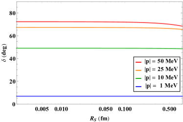
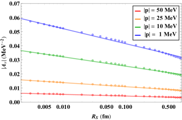
Figure 2: The left panel shows the phase shifts in the ${}^{1}S_{0}$ channel for several momenta $|{\mathbf{p}}|$ as functions of the cutoff, $R_{S}$. The right panel shows the $0\nu\beta\beta$ amplitude of Eq. (8). The dots result from explicitly evaluating Eq. (8), while the straight lines are due to a fit of the form $\mathcal{A}_{\nu}=a+b\ln R_{S}$.

Having obtained the wavefunctions $\Psi_{nn}$ and $\Psi_{pp}$, all that is left is to evaluate the amplitude in Eq. (8). This expression only depends on the values of the LECs $g_{A}$ and $C(R_{S})$, and the effective neutrino mass $m_{\beta\beta}$. $C(R_{S})$ has been linked to the $N\!N$ scattering length and is thus known for each value of $R_{S}$. As $|\mathcal{A}_{\nu}(E)|^{2}$ is an observable (although experimentally it will be hard to measure!) it should not depend on the value of the regulator. The value of $\mathcal{A}_{\nu}(E)$ for various energies as a function of the regulator $R_{S}$ is shown in the right panel of Fig. 2. The amplitude is clearly not regulator independent and the dependence at small $R_{S}$ can be fitted with a $\ln R_{S}$ function. We will derive the form of this $R_{S}$ dependence in later sections. At larger $R_{S}$, power corrections in $R_{S}$ induce a deviation from this simple behavior.

The consequences of the dependence of $\mathcal{A}_{\nu}(E)$ on $R_{S}$ are severe. Such dependence implies that $m_{\beta\beta}$ cannot be directly obtained from a measurement of the $nn\rightarrow pp\,e^{-}e^{-}$ transition (or alternatively, $m_{\beta\beta}$ cannot be limited from an experimental upper bound on the transition rate) as the matrix element linking the measurement to $m_{\beta\beta}$ depends on the unphysical parameter $R_{S}$. While we have studied a very simple state of just two nucleons, the arguments and conclusions do not depend on it: the same $R_{S}$ dependence occurs in nuclear transitions as long as the corresponding nuclei are described in $\chi$EFT. In practice it might be difficult to observe this regulator dependence due to the nature of many-body calculations where regulators are often fixed or can only be varied in a small range. In this light, ab initio calculations on lighter nuclei can provide an important intermediate step.

Of course, in an EFT setting an observable that depends on the regulator simply indicates that there exists a counterterm with a corresponding LEC that absorbs the divergence. In the context of $0\nu\beta\beta$ the counterterm is provided by a short-range $nn\rightarrow pp\,e^{-}e^{-}$ interaction that adds a term to the neutrino transition operator

$$V_{\nu\,{\rm L}}\rightarrow V_{\nu\,{\rm L}}-2g^{\rm NN}_{\nu}\,\tau^{(1)+}\tau^{(2)+}\equiv V_{\nu\,\rm L}+V_{\nu\,\rm S},$$ (12)

where $g^{\rm NN}_{\nu}$ is the corresponding LEC. In Weinberg’s power counting Weinberg (1990, 1991) such an interaction appears at N²LO. Renormalization, however, requires it at LO. This is in agreement with what was already anticipated on general grounds in Ref. Pavón Valderrama and Phillips (2015) for other weak currents acting in the ${}^{1}S_{0}$ channel. The LEC $g^{\rm NN}_{\nu}(R_{S})$ depends on the regulator $R_{S}$ in such a way as to make $\mathcal{A}_{\nu}(E)$ regulator independent.

We stress that $g^{\rm NN}_{\nu}$ corresponds to a genuine new contribution due to high-momentum neutrino exchange involving inter-nucleon distances $R\hskip 1.99997pt\raisebox{2.15277pt}{$<$}\raisebox{-3.00003pt}{$\sim$}\hskip 1.99997pt\Lambda_{\chi}^{-1}$. It is an intrinsically two-nucleon effect beyond that of the radii of weak form factors, which also lead to a short-range neutrino potential but can be determined in principle from one-nucleon processes—one-nucleon form-factor radii are N²LO contributions unaffected by two-nucleon physics. In contrast, two-nucleon weak currents, also a higher-order effect, generate a neutrino potential involving three nucleons. Despite being a two-nucleon quantity, $g^{\rm NN}_{\nu}$ cannot be described by a modification of the $N\!N$ potential itself which, in this example, is already correctly renormalized. Likewise, $g^{\rm NN}_{\nu}$ is not part of the so-called “short-range correlations” Miller and Spencer (1976); Haxton and Stephenson (1984); Simkovic et al. (2009); Engel et al. (2011); Benhar et al. (2014), if the latter are intended to describe nucleon correlations missed in approaches built on independent-particle states. As we have seen, $g^{\rm NN}_{\nu}$ is needed even when we use fully correlated wavefunctions, which are exact solutions of the Schrödinger equation. In ab initio calculations, such as those described in Sec. VIII, the input should be the ${}^{1}S_{0}$ neutrino potential (12), not Eq. (7). In many-body calculations where an ab initio approach is not possible, the ${}^{1}S_{0}$ neutrino potential should still be Eq. (12), on top of the correlations necessary to produce good wavefunctions starting from an independent-nucleon basis. Now, short-range correlations can be viewed as a modification of the neutrino potential—see e.g. the discussion in Ref. Benhar et al. (2014). Missing correlations at distances $R\hskip 1.99997pt\raisebox{2.15277pt}{$>$}\raisebox{-3.00003pt}{$\sim$}\hskip 1.99997pt\Lambda_{\chi}^{-1}$ can thus be mocked up by a $g^{\rm NN}_{\nu}(R)$. However, the converse is in principle not true: a $g^{\rm NN}_{\nu}(R_{S}\hskip 1.99997pt\raisebox{2.15277pt}{$<$}\raisebox{-3.00003pt}{$\sim$}\hskip 1.99997pt\Lambda_{\chi}^{-1})$ cannot be replaced by correlations at distances where the nucleon can be considered a well-defined entity. The situation is analogous to $\beta$ decay, where two-nucleon weak currents and short-range correlations are both present even if each can be viewed as an “in-medium quenching” of $g_{A}$—see Refs. Pastore et al. (2018a); Gysbers et al. (2019) for recent discussions.

$g^{\rm NN}_{\nu}$ accounts for neutrino exchange between quarks taking place at the characteristic QCD scale, which is needed for the very definition of the neutrino potential between nucleons and requires input from QCD. Indeed, while it is fairly easy to obtain part of $g^{\rm NN}_{\nu}(R_{S})$ by demanding that $\mathcal{A}_{\nu}(E)$ be regulator independent, the finite contribution of $g^{\rm NN}_{\nu}$ to the amplitude cannot be so obtained. The only way to get the total value of $g^{\rm NN}_{\nu}(R_{S})$ is to fit to data—similar to how we obtained $C(R_{S})$ by fitting the $N\!N$ scattering length. Fitting to LNV data is for obvious reasons impossible at present, and even if there were data it would be undesirable: we want to use a nonzero $0\nu\beta\beta$ rate to infer the value of the neutrino Majorana mass. Fortunately there are ways out. We will argue in Sec. VII that the problems associated to light Majorana-neutrino exchange also affect another well-known long-range potential, the Coulomb potential. In that case, the corresponding counterterm can be fitted to data on electromagnetic isospin-violating processes. Chiral symmetry relates the electromagnetic counterterms to $g^{\rm NN}_{\nu}(R_{S})$, but at present this is insufficient to fully determine it. Nevertheless, this approach explicitly demonstrates the necessity of including $g^{\rm NN}_{\nu}$ at LO. An alternative is to match this counterterm to results from a direct nonperturbative QCD calculation, something which is imaginable with lattice QCD (LQCD) methods, both for light Majorana exchange Shanahan et al. (2017); Tiburzi et al. (2017); Feng et al. (2019); Cirigliano et al. (2019) and TeV-scale LNV mechanisms Nicholson et al. (2018); Monge-Camacho et al. (2019).

III Effective field theories

In this section we describe the EFTs that we employ to discuss LNV in the two-nucleon sector. In Sec. III.1 we introduce pionless EFT, an EFT without explicit pionic degrees of freedom that allows us to derive more explicit expressions for the $nn\rightarrow pp\,e^{-}e^{-}$ amplitude than in chiral EFT. In Sec. III.2 we restore pions, and discuss some of the problems associated with them. Finally, in Sec.  III.3 we describe long- and short-range LNV operators at leading orders.

III.1 Pionless EFT

Few-body systems characterized by momentum scales $p$ much smaller than the pion mass can be described in pionless EFT (${/\pi}$EFT) Bedaque and van Kolck (1998); Bedaque et al. (1998); Chen et al. (1999); Kong and Ravndal (2000); Bedaque et al. (2000)—for a review, see Ref. Bedaque and van Kolck (2002). ${/\pi}$EFT has been shown to converge very well in the two- Chen et al. (1999); Kong and Ravndal (2000) and three- Vanasse (2013); König et al. (2016) nucleon sectors, and works within LO error bars for nuclei as large as ⁴⁰Ca Platter et al. (2005); Stetcu et al. (2007); Contessi et al. (2017); Bansal et al. (2018). While it is unclear whether its regime of validity extends to experimentally relevant $0\nu\beta\beta$ emitters, LNV amplitudes in ${/\pi}$EFT have a simple form, which allows analytical insight on the structure of the $0\nu\beta\beta$ transition operator Cirigliano et al. (2018b). Lowest-order interactions contribute only to $N\!N$ $S$ waves. Since the ${}^{1}S_{0}$ channel is the most important for $0\nu\beta\beta$, we will see that many conclusions drawn in ${/\pi}$EFT continue to hold in $\chi$EFT. Furthermore, ${/\pi}$EFT will be useful in light of a possible matching to LQCD calculations of $0\nu\beta\beta$ matrix elements performed at heavy pion masses. A similar matching between LQCD and ${/\pi}$EFT for strong and electroweak processes has been carried out in Refs. Barnea et al. (2015); Beane et al. (2015); Kirscher et al. (2015); Savage et al. (2017); Contessi et al. (2017); Shanahan et al. (2017); Tiburzi et al. (2017); Bansal et al. (2018).

The strong-interaction Lagrangian in ${/\pi}$EFT is made out of all interactions among nucleons—the relevant low-energy degrees of freedom in this case—constrained only by the symmetries of QCD. While an infinite set of such interactions exist, they can be ordered in a power-counting scheme. At LO in the two-nucleon ${}^{1}S_{0}$ channel,

$$\mathcal{L}^{(0)}_{{/\pi}}=\bar{N}\left(i\partial_{0}-\frac{\bm{\nabla}^{2}}{2m_{N}}\right)N-C\left(N^{T}{\vec{P}}_{{}^{1}S_{0}}N\right)^{\dagger}\cdot\left(N^{T}{{\vec{P}}}_{{}^{1}S_{0}}N\right),$$ (13)

where the nucleon isospin doublet is represented by $N=(p\;n)^{T}$ and the projector is

$$P^{a}_{{}^{1}S_{0}}=\frac{1}{\sqrt{8}}\tau_{2}\tau^{a}\sigma_{2}.$$ (14)

Here $\tau^{a}$ are the Pauli matrices in isospin space, where a vector is denoted by an arrow. The four-nucleon interaction scales as $C=\mathcal{O}(4\pi/(m_{N}\aleph))$ where $\aleph$ is a fine-tuned scale much smaller than the breakdown scale $\Lambda_{{/\pi}}\sim m_{\pi}$, in order to produce a low-energy pole in the $N\!N$ ${}^{1}S_{0}$ amplitude. At momenta $Q\sim\aleph$, the LO amplitude consists of a resummation of $C$ interactions, and coincides with that of the effective-range expansion truncated at the level of the scattering length. $C$ can thus be determined from matching to the $N\!N$ ${}^{1}S_{0}$ scattering length $a=-23.714$ fm or to the position of the virtual state in the complex momentum plane, which agree within the relative LO error $\sim r_{0}/a$ set by the effective range $r_{0}=2.7$ fm. The latter arises from the NLO Lagrangian

$$\mathcal{L}^{(1)}_{{/\pi}}=+\frac{C_{2}}{8}\left(N^{T}{\vec{P}}_{{}^{1}S_{0}}\overleftrightarrow{\bm{\nabla}}^{2}N\right)\cdot\left(N^{T}{\vec{P}}_{{}^{1}S_{0}}N\right)^{\dagger}+\textrm{H.c.}\,,$$ (15)

where $\overleftrightarrow{\bm{\nabla}}=\overrightarrow{\bm{\nabla}}-\overleftarrow{\bm{\nabla}}$ and $C_{2}$ scales as $C_{2}=\mathcal{O}(4\pi/(m_{N}\aleph^{2}\Lambda_{{/\pi}}))$.

To ensure regulator independence of the scattering amplitude, the LECs $C$ and $C_{2}$ must obey renormalization-group equations (RGEs). For example, in the power divergence subtraction (PDS) scheme Kaplan et al. (1998a, b),

$$\frac{d}{d\ln\mu}C=\frac{\mu m_{N}}{4\pi}C^{2},\qquad\frac{d}{d\ln\mu}\left(\frac{C_{2}}{C^{2}}\right)=0,$$ (16)

where $\mu$ is the renormalization scale. Solving the RGEs determines

$$C=\frac{4\pi}{m_{N}}\frac{1}{1/a-\mu}\,,\qquad C_{2}=\frac{2\pi}{m_{N}}\frac{r_{0}}{\left(1/a-\mu\right)^{2}}\,.$$ (17)

Similar RGEs hold in schemes that employ momentum cutoffs with the replacement $\mu\rightarrow c\Lambda$, where $c$ a scheme-dependent constant. With such regulators one sees explicitly that the amplitude calculated from the Lagrangian (13) contains a residual cutoff dependence, which contributes $\propto k^{2}/\Lambda$ to the effective-range expansion, with $k$ the on-shell momentum. This indicates that in the absence of further fine tuning $C_{2}$ enters at NLO and $r_{0}=\mathcal{O}(\Lambda_{{/\pi}}^{-1})$, consistent with its numerical value. Renormalization beyond LO can only be achieved if subleading corrections such as $C_{2}$ are treated in perturbation theory Beane et al. (1998); van Kolck (1999).

At higher orders a four-derivative operator appears whose coefficient, $C_{4}$, is fixed at N²LO and determined by the shape parameter at N³LO. Except for interactions in the ${}^{3}S_{1}$ channel analogous to those above, all other two-nucleon interactions contribute at N²LO or higher, including interactions in other isospin-triplet channels relevant to $0\nu\beta\beta$ such as ${}^{3}P_{0}$. The power counting is reviewed in Ref. Bedaque and van Kolck (2002). While our work focuses on the two-body sector, it is interesting that three-body forces appear already at LO in ${/\pi}$EFT Bedaque et al. (1999a, b, 2000). To our knowledge, the possible implications for the $0\nu\beta\beta$ transition operators have not been studied.

III.2 Chiral EFT

The low-energy EFT of QCD that incorporates pions explicitly is often called chiral EFT, a generalization of chiral perturbation theory ($\chi$PT) Weinberg (1979b) to systems with more than one nucleon Weinberg (1990, 1991). Pions play an important role as they emerge as pseudo-Goldstone bosons of the spontaneously broken, approximate chiral symmetry of QCD. This symmetry would be exact were it not for the small quark masses and electromagnetic charges. Contrary to ${/\pi}$EFT, in whose regime it is badly broken, approximate chiral symmetry is implemented in the $\chi$EFT Lagrangian: all interactions either conserve chiral symmetry or break it in the same way as the chiral-breaking sources at the quark level. In addition to the nucleon contact interactions of ${/\pi}$EFT, there are also pion interactions with nucleons and pions themselves. Because the Delta isobar is heavier than the nucleon by only about 300 MeV, it should also be included in order not to limit the range of validity of the theory too stringently Pandharipande et al. (2005). However, Delta isobars appear only in loops in the nuclear potential at orders higher than our discussion of renormalization below Ordonez et al. (1994, 1996), and will not be explicitly displayed. “Chiral potentials” obtained from $\chi$EFT—for a review, see Ref. Machleidt and Entem (2011)—have been extensively used as input to modern ab initio methods. It is hoped that $\chi$EFT converges for the nuclei employed in searches for $0\nu\beta\beta$.

For processes with at most one nucleon, $\chi$EFT can be treated in perturbation theory ($\chi$PT) in a systematic expansion in the small ratio $\epsilon_{\chi}$, Eq. (4) Weinberg (1979b). However, as in ${/\pi}$EFT, the existence of nuclei requires a resummation of a class of diagrams. In Weinberg’s original papers Weinberg (1990, 1991), it was recognized that the nonperturbative nature of $N\!N$ interactions is due to an infrared enhancement in the propagation of nucleons, leading to the presence of the large nucleon mass $m_{N}$ in the numerator of integrals arising from loops with only nucleons in intermediate states—a pinch singularity when $m_{N}\to\infty$. Weinberg then proposed to calculate nuclear amplitudes in two steps. In the first step one calculates a nuclear potential from diagrams that do not contain pinch singularities. Such diagrams are expected to follow the standard $\chi$PT power-counting rules, as long as nucleon contact interactions obey NDA Manohar and Georgi (1984). In a second step, the truncated nuclear potential is iterated to all orders by solving the Schrödinger equation. Most work on nuclear physics has followed this prescription.

While the potential in ${/\pi}$EFT consists of only contact interactions—all loops contain pinch singularities—in $\chi$EFT the potential contains also pion exchange. In Weinberg’s original prescription Weinberg (1990, 1991), static one-pion exchange (OPE) appears at LO in the potential,

$$V_{\pi}({\mathbf{q}})=-\frac{g_{A}^{2}}{12F_{\pi}^{2}}\,\mbox{${\vec{\tau}}$}^{(1)}\cdot\mbox{${\vec{\tau}}$}^{(2)}\left[\left(1-\frac{m_{\pi}^{2}}{{\mathbf{q}}^{\,2}+m_{\pi}^{2}}\right)\mbox{\boldmath$\sigma$}^{(1)}\cdot\mbox{\boldmath$\sigma$}^{(2)}-\frac{{\mathbf{q}}^{2}}{{\mathbf{q}}^{\,2}+m_{\pi}^{2}}S^{(12)}\right],$$ (18)

which is treated nonperturbatively together with contact interactions that arise from dynamics of shorter range than $m_{\pi}^{-1}$. The size of the contact LECs was assumed to be given by NDA, so at LO only two non-derivative, chiral-symmetric contact interactions were supposed to appear, one in ${}^{1}S_{0}$, the other in ${}^{3}S_{1}$. The question of renormalizability of the $N\!N$ amplitude was left unanswered. Initial numerical evidence Ordonez et al. (1994, 1996) suggested no problems. Unfortunately, it has been known from the mid-90s that Weinberg’s prescription leads to amplitudes that depend sensitively on the regularization procedure. Two types of problems have been identified:

1. In the ${}^{1}S_{0}$ channel, the LO potential reduces to Eqs. (10) and (11). According to NDA, $C$ consists of a contribution from pions plus the undetermined LEC $C_{0}$ of a chiral-symmetric contact interaction. The contact interaction is singular and must be renormalized. As we have seen in Sec. II, allowing $C$ to be cutoff dependent is sufficient for renormalization at a fixed pion mass. However, Ref. Kaplan et al. (1996) showed that the cutoff dependence contains an $m_{\pi}^{2}$-dependent logarithmic divergence that originates in the interference between the contact and Yukawa interactions. The presence of additional chiral-symmetry-breaking interactions is thus required for renormalization, even though such interactions appear at higher orders in Weinberg’s power counting. In a cutoff scheme, an operator with LEC $D_{2}m_{\pi}^{2}$ is sufficient to produce an $N\!N$ amplitude that approaches a constant as the cutoff is increased Beane et al. (2002), so that

   $$C=C_{0}+D_{2}\,m_{\pi}^{2}+\frac{g_{A}^{2}}{4F^{2}_{\pi}}.$$ (19)

2. In each attractive triplet wave where OPE is iterated, its $-r^{-3}$ singularity in coordinate space requires a chiral-symmetric contact interaction for renormalization Nogga et al. (2005); Pavón Valderrama and Ruiz Arriola (2006). While in the ${}^{3}S_{1}$-${}^{3}D_{1}$ coupled channels such an interaction is already predicted by NDA, in other waves it only appears at higher orders in Weinberg’s power counting. It is at present unclear in which waves OPE must be iterated. A semi-analytical argument Birse (2006) implies that $D$ waves and higher can be treated perturbatively, while Refs. Wu and Long (2019); Kaplan (2019) suggest even ${}^{3}P_{2}$-${}^{3}F_{2}$ is perturbative. Unfortunately, treating pion exchange perturbatively Kaplan et al. (1998a, b) does not work in the low triplet waves Fleming et al. (2000); Kaplan (2019).

In summary, for the isospin-triplet channels relevant for $0\nu\beta\beta$, the LO strong-interaction Lagrangian is

$$\mathcal{L}^{(0)}_{\chi} = \frac{1}{2}\partial_{\mu}{\vec{\pi}}\cdot\partial^{\mu}{\vec{\pi}}-\frac{1}{2}m_{\pi}^{2}{\vec{\pi}}^{2}+\bar{N}\left(i\partial_{0}-\frac{\bm{\nabla}^{2}}{2m_{N}}\right)N-\frac{g_{A}}{2F_{\pi}}\bm{\nabla}{\vec{\pi}}\cdot\bar{N}\mbox{${\vec{\tau}}$}\mbox{\boldmath$\sigma$}N$$ (20)

$$-\left(C_{0}+m_{\pi}^{2}D_{2}\right)\left(N^{T}{\vec{P}}_{{}^{1}S_{0}}N\right)^{\dagger}\cdot\left(N^{T}{\vec{P}}_{{}^{1}S_{0}}N\right)-C_{{}^{3}P_{0}}\left(N^{T}{\vec{P}}_{{}^{3}P_{0}}N\right)^{\dagger}\cdot\left(N^{T}{\vec{P}}_{{}^{3}P_{0}}N\right)$$

$$+\dots,$$

where ${\vec{\pi}}$ stands for the pion isospin triplet, the projector $P_{{}^{1}S_{0}}$ is defined in Eq. (14), the projector on the ${}^{3}P_{0}$ channel is

$${\vec{P}}_{{}^{3}P_{0}}=-\frac{i}{\sqrt{8}}\sigma_{2}\mbox{\boldmath$\sigma$}\cdot\overleftrightarrow{\bm{\nabla}}\tau_{2}\mbox{${\vec{\tau}}$},$$ (21)

and the dots denote terms with additional pion fields that are not relevant for our purposes. (Note, however, that these terms differentiate between $m_{\pi}^{2}D_{2}$ and $C_{0}$, so in higher orders or in processes with external pions these LECs do not always appear in the combination $C_{0}+m_{\pi}^{2}D_{2}$.) In $\chi$PT, as well as in the nuclear potential, one can demote the nucleon recoil term to NLO. The remaining terms on the first line of Eq. (20) give rise to the static OPE potential (18). The LECs $C_{0}$ and $m_{\pi}^{2}D_{2}$ contribute to Eq. (19), while $C_{{}^{3}P_{0}}$ ensures the renormalization of the ${}^{3}P_{0}$ wave at LO. The scaling $C_{0}=\mathcal{O}(4\pi/(m_{N}Q))$ is the same as in NDA and ${/\pi}$EFT, but the LECs $D_{2}\sim C_{{}^{3}P_{0}}=\mathcal{O}(4\pi/(m_{N}Q^{3}))$ are enhanced with respect to NDA by $\epsilon_{\chi}^{-2}$.

By consideration of the corrections in the ${}^{1}S_{0}$ channel similar to that done in the previous section, one finds Long and Yang (2012) that a nonvanishing NLO correction—that is, one order down in the expansion parameter $\epsilon_{\chi}$— exists despite being expected only two orders down the expansion in Weinberg’s power counting. The NLO strong-interaction Lagrangian can thus be written just as in ${/\pi}$EFT as

$$\mathcal{L}^{(1)}_{\chi}=+\frac{1}{8}C_{2}\left(N^{T}{\vec{P}}_{{}^{1}S_{0}}\overleftrightarrow{\bm{\nabla}}^{2}N\right)\cdot\left(N^{T}{\vec{P}}_{{}^{1}S_{0}}N\right)^{\dagger}+\textrm{H.c.},$$ (22)

with $C_{2}=\mathcal{O}(4\pi/(m_{N}Q^{2}\Lambda_{\chi}))$. It leads to an NLO correction to the LO potential in Eq. (11), given by

$$V_{N\!N}^{{}^{1}S_{0}(1)}({\mathbf{p}},{\mathbf{p}}^{\prime})=C^{(1)}+C_{2}\,\frac{{\mathbf{p}}^{2}+{\mathbf{p}}^{\prime\,2}}{2},$$ (23)

where $C^{(1)}=\mathcal{O}(4\pi/(m_{N}\Lambda_{\chi}))$ denotes a subleading component of the nonderivative operator defined in Eq. (20). Again as in ${/\pi}$EFT, this potential and other subleading interactions can only be renormalized in perturbation theory, in stark contrast to Weinberg’s prescription.

While the renormalization issues with Weinberg’s prescription have been extensively documented, there has been relatively little work done in applying properly renormalized $\chi$EFT to nuclear physics. It has in fact been argued that “chiral potentials” derived and treated according to Weinberg’s prescription give rise to better phenomenology, as long as the cutoff is chosen somewhat, but not too far, below the breakdown scale Epelbaum and Meissner (2013). The drawbacks of Weinberg’s prescription have limited impact on our conclusions below about the renormalization of the $0\nu\beta\beta$ amplitude. Our main results concern ${}^{1}S_{0}$ transitions at LO, as discussed in Sec. IV. The enhancement of $D_{2}$ has implications on the chiral properties of the contact in Eq. (12), but does not affect its existence in the first place. In Sec. V we show that the presence of counterterms in attractive triplet channels has no additional implications for the renormalization of the $0\nu\beta\beta$ amplitude. The effects of NLO corrections will be considered in Sec. VI.

III.3 Lepton-number-violating operators

The quark-level Lagrangian that is relevant to $0\nu\beta\beta$ transitions induced by a light Majorana neutrino is given in Eq. (2), and its matching onto $\chi$EFT is sketched in Eq. (3). The first ingredient required to derive the neutrino potential is the weak current $\mathcal{J}^{\mu}(\pi,N)$. $\mathcal{J}^{\mu}$ has vector and axial components, and it is dominated by one-body contributions. Writing

$$\mathcal{J}^{\mu}=\frac{1}{2}\bar{N}\tau^{+}\left[J_{V}^{\mu}+J_{A}^{\mu}\right]N+\ldots,$$ (24)

where $\ldots$ denote two- and higher-body contributions, the expressions of $J_{V}$ and $J_{A}$ through NLO in the chiral expansion are

$$J^{\mu}_{V} = g_{V}({\mathbf{q}}^{2})\left(v^{\mu}+\frac{p^{\mu}+p^{\prime\mu}}{2m_{N}}\right)+ig_{M}({\mathbf{q}}^{2})\,\epsilon^{\mu\nu\alpha\beta}\,\frac{v_{\alpha}S_{\beta}q_{\nu}}{m_{N}}\,,$$

$$J^{\mu}_{A} = -2g_{A}({\mathbf{q}}^{2})\left(S^{\mu}-\frac{S\cdot(p+p^{\prime})}{2m_{N}}\,v^{\mu}+\frac{S\cdot q}{{\mathbf{q}}^{2}+m_{\pi}^{2}}\,q^{\mu}\right)\,.$$ (25)

Here $p$ and $p^{\prime}$ stand for the momentum of the incoming neutron and outgoing proton, respectively, $q^{\mu}=(q^{0},\,{\mathbf{q}})=p^{\mu}-p^{\prime\mu}$, and $v^{\mu}$ and $S^{\mu}$ are respectively the nucleon velocity and spin ($v^{\mu}=(1,\,{\mathbf{0}})$ and $S^{\mu}=(0,\,\mbox{\boldmath$\sigma$}/2)$ in the nucleon rest frame). Furthermore, $\epsilon^{\mu\nu\alpha\beta}$ is the totally antisymmetric tensor, with $\epsilon^{0123}=+1$. At LO, the vector, axial, and magnetic form factors are given by

$$g_{V}({\mathbf{q}}^{2}) = g_{V}=1\,,\qquad g_{A}({\mathbf{q}}^{2})=g_{A}\simeq 1.27\,,\qquad g_{M}({\mathbf{q}}^{2})=1+\kappa_{1}\simeq 4.7\,,$$ (26)

where $\kappa_{1}\simeq 3.7$ is the nucleon isovector anomalous magnetic moment. In the literature, the momentum dependence of the vector and axial form factors, and the contribution of weak magnetism to the neutrino potential are usually included—see for example Ref. Engel and Menéndez (2017). Since these are N²LO effects, we will neglect them in most of the paper.

Equation (III.3) can be used to derive the long-range component of the $0\nu\beta\beta$ transition operator given in Eq. (6). The expression in ${/\pi}$EFT can be obtained by taking the $m_{\pi}\rightarrow\infty$ limit in Eq. (6). In this limit, the tensor component of $V_{\nu}$ vanishes. The most singular part of $V_{\nu}$, which we denote by $\tilde{V}$, has a $1/{\mathbf{q}}^{2}$ behavior. The projections on the waves discussed in this paper are

$$\tilde{V}_{\nu\,{\rm L}}^{{}^{1}S_{0}}({\mathbf{q}})=\tilde{V}_{\nu\,{\rm L}}^{{}^{1}D_{2}}({\mathbf{q}})=\tau^{(1)+}\tau^{(2)+}\,\frac{1+2g_{A}^{2}}{{\mathbf{q}}^{2}},\qquad\tilde{V}_{\nu\,\rm L}^{{}^{3}P_{J}}({\mathbf{q}})=\tau^{(1)+}\tau^{(2)+}\,\frac{1}{{\mathbf{q}}^{2}}\left(1-\frac{2}{3}g_{A}^{2}-\frac{g_{A}^{2}}{3}S^{(12)}|_{{}^{3}P_{J}}\right),$$ (27)

where the tensor operator in Eq. (27) is meant to be projected in the appropriate $P$ wave, as discussed in more detail in Sec. V. In ${/\pi}$EFT Eq. (27) reduces to

$$\tilde{V}_{\nu\,\rm L}^{{}^{1}S_{0}}({\mathbf{q}})=\tilde{V}_{\nu\,\rm L}^{{}^{1}D_{2}}({\mathbf{q}})=\tau^{(1)+}\tau^{(2)+}\,\frac{1+3g_{A}^{2}}{{\mathbf{q}}^{2}},\qquad\tilde{V}_{\nu\,\rm L}^{{}^{3}P_{J}}({\mathbf{q}})=\tau^{(1)+}\tau^{(2)+}\,\frac{1-g_{A}^{2}}{{\mathbf{q}}^{2}}.$$ (28)

In coordinate space, the long-range neutrino potential defined in Eq. (6) is

$$V_{\nu\,\rm L}=\tau^{(1)+}\tau^{(2)+}\left(V_{F}(r)-g_{A}^{2}\,V_{GT}(r)\,{\bm{\sigma}}^{(1)}\cdot{\bm{\sigma}}^{(2)}-g_{A}^{2}\,V_{T}(r)\,S^{(12)}\right)\,,$$ (29)

where the tensor operator $S^{(12)}(\hat{r})\equiv 3\mbox{\boldmath$\sigma$}^{(1)}\cdot\hat{{\mathbf{r}}}\mbox{\boldmath$\sigma$}^{(2)}\cdot\hat{{\mathbf{r}}}-\mbox{\boldmath$\sigma$}^{(1)}\cdot\mbox{\boldmath$\sigma$}^{(2)}$ and the radial functions

$$V_{F}(r) = \frac{1}{4\pi r},\qquad V_{GT}(r)=\frac{1}{4\pi r}\left[1-\frac{e^{-m_{\pi}r}}{6}\left(2+m_{\pi}r\right)\right],$$

$$V_{T}(r) = \frac{1}{2\pi r(m_{\pi}r)^{2}}\left[1-e^{-m_{\pi}r}\left(1+m_{\pi}r+\frac{5}{12}(m_{\pi}r)^{2}+\frac{1}{12}(m_{\pi}r)^{3}\right)\right].$$ (30)

In various channels considered below,

$$V_{\nu\,{\rm L}}^{{}^{1}S_{0}}(r) = V_{\nu\,\rm L}^{{}^{1}D_{2}}(r)=\tau^{(1)+}\tau^{(2)+}\left(V_{F}(r)+3g_{A}^{2}\,V_{GT}(r)\right),$$ (31)

$$V_{\nu\,{\rm L}}^{{}^{3}P_{J}}(r) = \tau^{(1)+}\tau^{(2)+}\left(V_{F}(r)-g_{A}^{2}\,V_{GT}(r)+a_{J}g_{A}^{2}\,V_{T}(r)\right),$$ (32)

where $a_{0}=4$, $a_{1}=-2$ and $a_{2}=2/5$.

Of the remaining terms in Eq. (3), the operators schematically denoted by $\mathcal{O}$ induce LNV corrections to $\beta$ decay processes and long-range contributions to $0\nu\beta\beta$. $\mathcal{O}$ is produced at tree level by $SU(2)_{L}\times U(1)_{Y}$-invariant LNV operators of dimension seven and higher Cirigliano et al. (2017, 2018a). If one considers only LNV induced by a neutrino Majorana mass, however, these operators are suppressed by electroweak loops with respect to the leading contributions, and we will neglect them here.

The operators denoted by $\mathcal{O}^{\prime}$ represent local LNV interactions between nucleons, pions and electrons, which are induced either by operators of dimension nine and higher Prezeau et al. (2003); Graesser (2017); Cirigliano et al. (2017, 2018a) or by the exchange of hard Majorana neutrinos Cirigliano et al. (2018b). The latter operators have the same transformation properties as the product of two weak currents, and their construction is detailed in Sec. VII. For $0\nu\beta\beta$, the most important interaction is

$$\mathcal{L}_{|\Delta L|=2}^{NN}=-\left(2\sqrt{2}\,G_{F}V_{ud}\right)^{2}m_{\beta\beta}\,\bar{e}_{L}C\bar{e}_{L}^{T}\,g_{\nu}^{\rm NN}\left[(N^{T}P_{{}^{1}S_{0}}^{\,+}N)(N^{T}P_{{}^{1}S_{0}}^{\,-}N)^{\dagger}\right]+\textrm{H.c.}+\ldots\,,$$ (33)

where interactions with additional pion fields required by chiral symmetry are not written explicitly. Here the projectors $P_{{}^{1}S_{0}}^{\,\pm}$ are defined in terms of those in Eq. (14) as $P_{{}^{1}S_{0}}^{\,\pm}=(P_{{}^{1}S_{0}}^{\,1}\pm iP_{{}^{1}S_{0}}^{\,2})/2$. In Weinberg’s power counting, $g_{\nu}^{\rm NN}=\mathcal{O}((4\pi F_{\pi})^{-2})$ would contribute to the neutrino potential at N²LO. As we argued in Sec. II and will discuss in more detail in Sec. IV, the logarithmic dependence of LNV scattering amplitudes on the regulator induced by light-neutrino exchange requires $g_{\nu}^{\rm NN}$ to be promoted to LO, $g_{\nu}^{\rm NN}=\mathcal{O}(F_{\pi}^{-2})$ instead. In addition, Ref. Kaplan et al. (1996) demonstrated that an $m_{\pi}^{2}$ expansion might not be appropriate for four-nucleon operators. As we will explicitly show below, the counterterm needed for $0\nu\beta\beta$ inherits in $\chi$EFT some dependence on the quark mass. We need to construct $|\Delta L|=2$ operators with one and two insertions of the quark masses, which we discuss in detail in App. A. In the limit of equal up and down quark masses, $m_{u}=m_{d}$, considering insertions of the common quark mass leads to operators in the form of Eq. (33), but differing in the pion interactions lumped into the ellipsis. The coupling of the four-nucleon operator is replaced by

$$g_{\nu}^{\rm NN}=\sum_{n}g_{n}m_{\pi}^{2n},$$ (34)

where the coefficients $g_{n}$ scale as $\Lambda^{-2n-2}$, with $n=0,1,\ldots$ an integer. NDA suggests $\Lambda\sim\Lambda_{\chi}$, implying that the mass dependence is suppressed. We will however see that renormalization requires $g_{\nu}^{\rm NN}\propto C^{2}$, implying that, at least for $g_{1}$ and $g_{2}$, the scale $\Lambda$ should be $\Lambda\sim F_{\pi}$. In addition to the operator in Eq. (34), additional mass-dependent operators can be constructed, but they contain at least two pion fields as described in App. A.

Beyond LO, additional contact interactions contribute to $0\nu\beta\beta$. In Sec. VI we will consider the derivative operator

$$\mathcal{L}_{|\Delta L|=2}^{NN} = \left(2\sqrt{2}G_{F}V_{ud}\right)^{2}m_{\beta\beta}\,\bar{e}_{L}C\bar{e}_{L}^{T}\,\frac{g_{2\,\nu}^{\rm NN}}{8}$$ (35)

$$\times\left[(N^{T}\overleftrightarrow{\bm{\nabla}}^{2}P_{{}^{1}S_{0}}^{\,+}N)(N^{T}P_{{}^{1}S_{0}}^{\,-}N)^{\dagger}+(N^{T}P_{{}^{1}S_{0}}^{\,+}N)(N^{T}\overleftrightarrow{\bm{\nabla}}^{2}P_{{}^{1}S_{0}}^{\,-}N)^{\dagger}\right]+\textrm{H.c.},$$

which also acts between two ${}^{1}S_{0}$ waves , and we discuss the power counting for its LEC $g_{2\,\nu}^{\rm NN}$.

The contact interactions in Eqs. (33) and (35) give short-range contributions to the $0\nu\beta\beta$ transition operator. Factoring out $G_{F}$, $m_{\beta\beta}$ and the lepton fields as in Eq. (5), the short-range potential in the ${}^{1}S_{0}$ channel is

$$V_{\nu\,\rm S}({\mathbf{p}},{\mathbf{p}}^{\prime})=-2\tau^{(1)+}\,\tau^{(2)+}\left(g_{\nu}^{\rm NN}+g_{2\nu}^{\rm NN}\,\frac{{\mathbf{p}}^{2}+{\mathbf{p}}^{\prime\,2}}{2}\right).$$ (36)

It turns out that the short-distance operators induced by the exchange of hard neutrinos are related by isospin symmetry to isospin-two operators induced by the exchange of hard photons. In Sec. VII we will discuss this relation in detail, and explore its implications for $0\nu\beta\beta$.

IV The LNV scattering amplitude at leading order

In this section we study the $nn\rightarrow pp\,e^{-}e^{-}$ scattering amplitude at LO in the ${}^{1}S_{0}$ channel, and show how the need for a short-range component of the neutrino potential arises in ${/\pi}$EFT and $\chi$EFT. The section is based on the results of Refs. Cirigliano et al. (2018b, c), which we discuss in greater detail. We start by examining the amplitude in ${/\pi}$EFT in Sec. IV.1. This allows us to derive an analytic expression for the amplitude. In $\chi$EFT, the iteration of the pion-exchange Yukawa potential makes it impossible to provide a simple closed expression for the $nn\rightarrow pp\,e^{-}e^{-}$ scattering amplitude, but one can still identify the leading divergent behavior in dimensional regularization as we show in Sec. IV.2. However, dimensional regularization is rarely used in few-body calculations. In Sec. IV.3 we therefore perform the same analysis with cutoff schemes that are widely used in the literature.

The LO contributions to $nn\rightarrow pp\,e^{-}e^{-}$ from the exchange of a light neutrino are shown in the top panel of Fig. 3. The blue ellipse denotes the iteration of the Yukawa potential $V_{\pi}({\mathbf{q}})$, while the contact interaction comes from the LEC $C$. For the diagrams in the second and third row of Fig. 3, one has to include an infinite number of bubbles, dressed with iterations of the Yukawa potential. The diagrams for ${/\pi}$EFT can be obtained from those in Fig. 3 by neglecting the pion exchange potential. Without loss of generality for our arguments, we use the kinematics of Eq. (9), with the electrons emitted at zero momentum. For incoming neutrons with $|{\mathbf{p}}|=1$ MeV, the relative momentum of the outgoing protons is $|{\mathbf{p}}^{\prime}|\simeq 38$ MeV.

Figure 3: Diagrammatic representation of LO and NLO contributions to $nn\rightarrow pp\,e^{-}e^{-}$ induced by long-range neutrino exchange. Double, dashed, and plain lines denote nucleons, pions, and leptons, respectively. Gray circles denote the nucleon axial and vector currents, and the black square an insertion of $m_{\beta\beta}$. The blue ellipse represents iteration of $V_{\pi}$, while an unmarked contact interaction stands for $C$. In the NLO diagrams, the black circle denotes an insertion of $C_{2}$. Diagrams analogous to those in the second and fourth rows, but with contact interactions to the left of neutrino exchange, are not shown. The diagrams for ${/\pi}$EFT are obtained by neglecting pion exchange in the blue ellipse.

Following Refs. Kaplan et al. (1996); Long and Yang (2012), from the free Hamiltonian $H_{0}$ and the pion potential $V_{\pi}$ we introduce  the retarded ($+$) and advanced ($-$) propagators

$$\hat{G}^{\pm}_{E}=\frac{1}{E-H_{0}-V_{\pi}\pm i\varepsilon},\qquad G^{\pm}_{E}({\mathbf{r}},{\mathbf{r}}^{\prime})=\int\frac{d^{3}{\mathbf{k}}}{(2\pi)^{3}}\int\frac{d^{3}{\mathbf{k}}^{\prime}}{(2\pi)^{3}}\,e^{i{\mathbf{k}}\cdot r}e^{-i{\mathbf{k}}^{\prime}\cdot{\mathbf{r}}^{\prime}}\langle{\mathbf{k}}|\hat{G}^{\pm}_{E}|{\mathbf{k}}^{\prime}\rangle,$$ (37)

and the Yukawa “in” ($+$) and “out”($-$) wavefunctions

$$\chi^{\pm}_{{\mathbf{p}}}({\mathbf{r}}) = \int\frac{d^{3}{\mathbf{k}}}{(2\pi)^{3}}\,e^{i{\mathbf{k}}\cdot{\mathbf{r}}}\langle{\mathbf{k}}|(1+\hat{G}^{\pm}_{E}V_{\pi})|{\mathbf{p}}\rangle.$$ (38)

Reference Kaplan et al. (1996) shows that the bubble diagrams in Fig. 3 are related to $G^{+}_{E}({\mathbf{0}},{\mathbf{0}})=[G^{-}_{E}({\mathbf{0}},{\mathbf{0}})]^{*}$, while the triangles dressed by Yukawas are related to $\chi^{+}_{{\mathbf{p}}}({\mathbf{0}})$ and $\chi^{-}_{{\mathbf{p}}^{\prime}}({\mathbf{0}})^{*}=\chi^{+}_{{\mathbf{p}}^{\prime}}({\mathbf{0}})$ (see Fig. 5 in Ref. Kaplan et al. (1996)). It is also convenient to introduce

$$K_{E} = \frac{C}{1-CG^{+}_{E}({\mathbf{0}},{\mathbf{0}})}.$$ (39)

The divergence in $G^{+}_{E}({\mathbf{0}},{\mathbf{0}})$ is absorbed by $C^{-1}$, so that $K_{E}$ is well defined and scale/scheme independent Kaplan et al. (1996).

The chains of bubbles in the second and third rows of Fig. 3 can be resummed, and at LO the amplitude can be expressed as

$$\mathcal{A}^{\rm LO}_{\nu} = \mathcal{A}_{A}+\chi^{+}_{{\mathbf{p}}^{\prime}}({\mathbf{0}})\,K_{E^{\prime}}\,\mathcal{A}_{B}+\mathcal{\bar{A}}_{B}\,K_{E}\,\chi^{+}_{{\mathbf{p}}}({\mathbf{0}})+\chi^{+}_{{\mathbf{p}}^{\prime}}({\mathbf{0}})\,K_{E^{\prime}}\,\mathcal{A}_{C}\,K_{E}\,\chi^{+}_{{\mathbf{p}}}({\mathbf{0}}),$$ (40)

where $\mathcal{A}_{A}$, $\mathcal{A}_{B}$, and $\mathcal{A}_{C}$ denote the first diagram in the first, second, and third row of Fig. 3, respectively (without the wavefunctions at ${\mathbf{0}}$, in the case of $B$ and $C$), while $\mathcal{\bar{A}}_{B}$ stands for the analog of the second row where contact interactions come before neutrino exchange.

The contribution of the operator $g_{\nu}^{\rm NN}$, defined in Eq. (33), is shown in the first row of Fig. 4. It is easy to sum these diagrams, which modify the amplitude into

$$\mathcal{A}^{\rm LO}_{\nu} = \mathcal{A}_{A}+\chi^{+}_{{\mathbf{p}}^{\prime}}({\mathbf{0}})\,K_{E^{\prime}}\,\mathcal{A}_{B}+\mathcal{\bar{A}}_{B}\,K_{E}\,\chi^{+}_{{\mathbf{p}}}({\mathbf{0}})+\chi^{+}_{{\mathbf{p}}^{\prime}}({\mathbf{0}})\,K_{E^{\prime}}\left(\mathcal{A}_{C}+\frac{2g_{\nu}^{\rm NN}}{C^{2}}\right)K_{E}\,\chi^{+}_{{\mathbf{p}}}({\mathbf{0}}).$$ (41)

Since $g_{\nu}^{\rm NN}$ appears together with $C^{-2}$, it proves convenient to define the dimensionless parameter

$$\tilde{g}_{\nu}^{\rm NN}=\left(\frac{4\pi}{m_{N}C}\right)^{2}g_{\nu}^{\rm NN}.$$ (42)

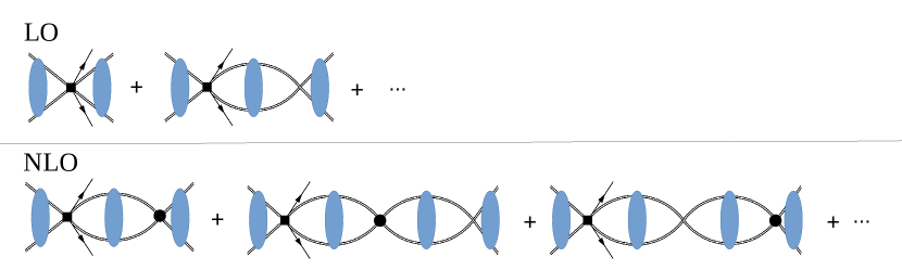
Figure 4: Diagrammatic representation of LO and NLO contributions to $nn\rightarrow pp\,e^{-}e^{-}$ induced by the short-range operator $g_{\nu}^{\rm NN}$. The notation is as in Fig. 3. The diagrams for ${/\pi}$EFT are obtained by neglecting pion exchange in the blue ellipse.

The amplitude has the same structure in ${/\pi}$EFT and $\chi$EFT. In ${/\pi}$EFT, $\mathcal{A}_{A}$, $\mathcal{A}_{B}$, $\bar{\mathcal{A}}_{B}$ and $\mathcal{A}_{C}$ contain a single diagram, which can be analytically computed in dimensional regularization. In $\chi$EFT, on the other hand, they still contain an infinite series of diagrams. We now examine the two theories in more detail.

IV.1 Pionless EFT

In ${/\pi}$EFT the Yukawa wavefunction $\chi_{{\mathbf{p}}}^{\pm}$ reduces to a plane wave, with $\chi_{{\mathbf{p}}}(0)=1$. ${G}_{E}^{+}({\mathbf{r}},{\mathbf{r}}^{\prime})$ is the free nucleon propagator,

$$\left({G}_{E}^{+}({\mathbf{0}},{\mathbf{0}})\right)_{{/\pi}}=-I_{0}({\mathbf{p}})=\int\frac{d^{d-1}k}{(2\pi)^{d-1}}\,\frac{m_{N}}{{\mathbf{p}}^{2}-{\mathbf{k}}^{2}+i\varepsilon}=-\frac{m_{N}}{4\pi}\left(\mu+i|{\mathbf{p}}|\right)$$ (43)

in $d$ spacetime dimensions, where in the last equality we have used the PDS scheme Kaplan et al. (1998a). $K_{E}$ reduces to the full strong scattering amplitude,

$$\left(K_{E}\right)_{{/\pi}}=-T^{(0)}_{{}^{1}S_{0}}=\frac{1}{C^{-1}+I_{0}({\mathbf{p}})}=\frac{4\pi}{m_{N}}\frac{1}{1/a+i|{\mathbf{p}}|}.$$ (44)

Equation (41) then becomes

$$\mathcal{A}_{\nu}^{\rm LO} = \mathcal{A}_{A}-\mathcal{A}_{B}({\mathbf{p}}^{2},{\mathbf{p}}^{\prime\,2})\,T^{(0)}_{{}^{1}S_{0}}({\mathbf{p}}^{\prime\,2})-T^{(0)}_{{}^{1}S_{0}}({\mathbf{p}}^{2})\,\bar{\mathcal{A}}_{B}({\mathbf{p}}^{2},{\mathbf{p}}^{\prime\,2})$$ (45)

$$+T^{(0)}_{{}^{1}S_{0}}({\mathbf{p}}^{2})\left(\mathcal{A}_{C}({\mathbf{p}}^{2},{\mathbf{p}}^{\prime\,2})+\frac{2g_{\nu}^{\rm NN}}{C^{2}}\right)T^{(0)}_{{}^{1}S_{0}}({\mathbf{p}}^{\prime\,2}).$$

Here $\mathcal{A}_{A}$ is the projection of the neutrino potential in the ${}^{1}S_{0}$ channel,

$$\mathcal{A}_{A}=-\frac{1+3g_{A}^{2}}{2}\int d\cos\theta\,\frac{1}{({\mathbf{p}}-{\mathbf{p}}^{\prime})^{2}},$$ (46)

with $\theta$ the angle between ${\mathbf{p}}$ and ${\mathbf{p}}^{\prime}$, while $\mathcal{A}_{B}$ and $\mathcal{A}_{C}$ reduce to one- and two-loop integrals,

$${\mathcal{A}}_{B}({\mathbf{p}}^{\prime 2},{\mathbf{p}}^{2}) = \bar{\mathcal{A}}_{B}({\mathbf{p}}^{2},{\mathbf{p}}^{\prime\,2})=-m_{N}\int\frac{d^{d-1}k}{(2\pi)^{d-1}}\,\frac{1}{{\mathbf{p}}^{2}-{\mathbf{k}}^{2}+i\varepsilon}\,\frac{1+3g_{A}^{2}}{({\mathbf{k}}-{\mathbf{p}}^{\prime})^{2}},$$ (47)

$$\mathcal{A}_{C}({\mathbf{p}}^{2},{\mathbf{p}}^{\prime\,2}) = -m_{N}^{2}\int\frac{d^{d-1}k}{(2\pi)^{d-1}}\int\frac{d^{d-1}q}{(2\pi)^{d-1}}\,\frac{1}{{\mathbf{p}}^{2}-{\mathbf{k}}^{2}+i\varepsilon}\,\frac{1+3g_{A}^{2}}{({\mathbf{k}}-{\mathbf{q}})^{2}}\,\frac{1}{{\mathbf{p}}^{\prime\,2}-{\mathbf{q}}^{2}+i\varepsilon}.$$ (48)

$\mathcal{A}_{B}$ is UV finite, and for $|{\mathbf{p}}^{\prime}|>|{\mathbf{p}}|$ it is given by

$$\bar{\mathcal{A}}_{B}({\mathbf{p}}^{2},{\mathbf{p}}^{\prime\,2})=\frac{m_{N}}{4\pi}\,\frac{1+3g_{A}^{2}}{2}\,\frac{i}{|{\mathbf{p}}^{\prime}|}\ln\frac{|{\mathbf{p}}|+|{\mathbf{p}}^{\prime}|}{|{\mathbf{p}}|-|{\mathbf{p}}^{\prime}|+i0^{+}}.$$ (49)

On the other hand, $\mathcal{A}_{C}$ is logarithmically divergent,

$${\mathcal{A}}_{C}({\mathbf{p}}^{2},{\mathbf{p}}^{\prime\,2})=-\left(\frac{m_{N}}{4\pi}\right)^{2}\frac{1+3g_{A}^{2}}{2}\left(\frac{1}{4-d}-\gamma+\ln 4\pi+2L_{{\mathbf{p}},{\mathbf{p}}^{\prime}}(\mu)\right)~{},$$ (50)

where $\gamma$ is the Euler-Mascheroni constant and, in the PDS scheme,

$$L_{{\mathbf{p}},\,{\mathbf{p}}^{\prime}}(\mu)=\frac{1}{2}\left(\ln\frac{\mu^{2}}{-4(|{\mathbf{p}}|+|{\mathbf{p}}^{\prime}|)^{2}-i0^{+}}+1\right).$$ (51)

Equations (45) and (50) clearly show that the scattering amplitude $\mathcal{A}_{\nu}$ is UV divergent unless $g_{\nu}^{\rm NN}$ appears at LO. Moreover, Eq. (45) allows one to derive the RGE for $g_{\nu}^{\rm NN}$ or equivalently for $\tilde{g}_{\nu}^{\rm NN}$ (see Eq. (42))

$$\frac{d}{d\ln\mu}\tilde{g}_{\nu}^{\rm NN}=\frac{1+3g_{A}^{2}}{2}\equiv\beta.$$ (52)

The solution is

$$\tilde{g}_{\nu}^{\rm NN}(\mu)=\beta\,\ln(\mu/\mu_{0})+\tilde{g}_{\nu}^{\rm NN}(\mu_{0}),$$ (53)

with an initial condition $\tilde{g}_{\nu}^{\rm NN}(\mu_{0})$ at some scale $\mu_{0}$. There might be a scale $\mu_{0}$ for which $\tilde{g}_{\nu}^{\rm NN}(\mu_{0})\ll 1$ rather than $\mathcal{O}(1)$. However, at a comparable scale $\mu_{0}+\delta\mu_{0}$ with $\delta\mu_{0}\sim\mu_{0}$, $\tilde{g}_{\nu}^{\rm NN}(\mu_{0}+\delta\mu_{0})={\mathcal{O}}(\beta)$. Thus, it is natural to assume that $g_{\nu}^{\rm NN}=\mathcal{O}(1/\aleph^{2})$ Cirigliano et al. (2018b) as expected from the fact that $g_{\nu}^{\rm NN}$ connects two S waves Bedaque and van Kolck (2002).

Similar expressions can be obtained in cutoff schemes, if loop diagrams are regulated in such a way that multiple loops with the insertion of contact interactions factorize into a product of one-loop diagrams, thus allowing the bubbles to be resummed. This happens for “separable” regulators in the form of a product of a function of the incoming momentum (${\mathbf{p}}$) and a function of the outgoing momentum (${\mathbf{p}}^{\prime}$). One example, which will be used in the following sections, is when contact interactions such as $C$ and $C_{2}$ are replaced,

$$C\rightarrow f(|{\mathbf{p}}^{\prime}|/\Lambda)\,C\,f(|{\mathbf{p}}|/\Lambda)$$ (54)

where $f$ is a function such that $f(0)=1$ and $f(\infty)=0$, and $\Lambda$ is the cutoff parameter. For separable regulators, $\mathcal{A}_{\nu}^{\rm LO}$ still has the expression given in Eq. (45). It exhibits a logarithmic dependence on the cutoff $\Lambda$, and the same argument for the presence of $\tilde{g}_{\nu}^{\rm NN}$ at LO goes through.

The non-separable regulator we will consider here involves the transferred momentum which produces a regularization of the three-dimensional delta function in coordinate space,

$$\delta^{(3)}({\mathbf{r}})\rightarrow\delta^{(3)}_{R_{S}}({\mathbf{r}})\,,$$ (55)

where $R_{S}$ is a cutoff parameter such that $\lim_{R_{S}\to 0}\delta^{(3)}_{R_{S}}({\mathbf{r}})=\delta^{(3)}({\mathbf{r}})$. For non-separable regulators, one has to resort to numerical calculations even in the two-nucleon sector of ${/\pi}$EFT. In numerical calculations, where negative powers of $\Lambda$ cannot be isolated and simply dropped, the cutoff parameter should be taken beyond the EFT breakdown scale so that cutoff artifacts are no larger than the effects of higher-order LECs. We note that while we have only sketched the calculation of LNV amplitudes in ${/\pi}$EFT with cutoff regulators, they can be obtained with the numerical procedure of Sec. IV.3, by setting $g_{A}\to 0$ in the strong potential.

IV.2 Chiral EFT with dimensional regularization

In $\chi$EFT, $\mathcal{A}_{A}$, $\mathcal{A}_{B}$, $\bar{\mathcal{A}}_{B}$, and $\mathcal{A}_{C}$ contain an infinite sum of diagrams. In order to study the renormalization of the neutrino potential, let us discuss the divergence structure of ${\mathcal{A}}_{\nu}$. We note that:

• All the diagrams in $\mathcal{A}_{A}$ are finite. The tree level is obviously finite, as Eq. (46) in ${/\pi}$EFT. Each iteration of the Yukawa interaction brings in a factor of $d^{3}{\mathbf{k}}/({\mathbf{k}}^{2})^{2}$, where one ${\mathbf{k}}^{-2}$ comes from the pion propagator, the other from the two-nucleon propagators after integrating over $k_{0}$. So, every Yukawa insertion improves the convergence.

• All the diagrams in $\mathcal{A}_{B}$ and $\bar{\mathcal{A}}_{B}$ are finite as well. The first loop is similar to the result in ${/\pi}$EFT, Eq. (47), which is finite. Again, insertions of the Yukawa interaction improve the convergence.

• The first two-loop diagram in $\mathcal{A}_{C}$ is logarithmically divergent. The divergence arises from insertion of the most singular component of the neutrino potential, namely $\tilde{V}_{\nu}^{{}^{1}S_{0}}$ defined in Eq. (27). This is analogous to Eq. (48) in ${/\pi}$EFT. The two-loop diagram with an insertion of $V_{\nu}-\tilde{V}_{\nu}$ and higher-loop diagrams with one or more Yukawa insertions are convergent.

We thus focus on $\mathcal{A}_{C}\equiv\mathcal{A}_{C}^{\rm sing}+\delta\mathcal{A}_{C}$. The singular two-loop diagram $\mathcal{A}_{C}^{\rm sing}$ is the same as in ${/\pi}$EFT, with $1+3g_{A}^{2}\rightarrow 1+2g_{A}^{2}$ due to the pion contribution to the induced pseudoscalar form factor. The renormalized amplitude in the PDS and $\overline{\rm MS}$ schemes is obtained by the replacement

$$\mathcal{A}_{C}+\frac{2g_{\nu}^{\rm NN}}{C^{2}}\to\left(\frac{m_{N}}{4\pi}\right)^{2}\left[2\tilde{g}_{\nu}^{\rm NN}(\mu)-\left(1+2g_{A}^{2}\right)L_{{\mathbf{p}},\,{\mathbf{p}}^{\prime}}(\mu)\right]+\delta\mathcal{A}_{C}$$ (56)

in Eq. (41). Instead of Eq. (52), the renormalized coupling obeys the RGE

$$\frac{d}{d\ln\mu}\tilde{g}_{\nu}^{\rm NN}=\frac{1+2g_{A}^{2}}{2}~{}.$$ (57)

The above argument shows that, as in ${/\pi}$EFT, the counterterm $g_{\nu}^{\rm NN}=\mathcal{O}(1/Q^{2})$ must be included at LO in Eq. (41).

The finite part of the coupling can be obtained in principle by matching the S-matrix element in Eqs. (41) and (56) to a LQCD calculation, performed at the same kinematic point. In order to carry out this program, one needs a non-perturbative calculation of the S-matrix element in $\chi$EFT, which amounts to a resummation of the infinite number of Feynman diagrams building up to $\mathcal{A}_{A}$, $\mathcal{A}_{B}$ and $\delta\mathcal{A}_{C}$. This is equivalent to solving the Schrödinger equation Kaplan et al. (1996), as we recall below.

One can re-express the amplitudes in Fig. 3 as

$$\mathcal{A}_{A} = -\int d^{3}{\mathbf{r}}\,\chi^{-}_{{\mathbf{p}}^{\prime}}({\mathbf{r}})^{*}\,V_{\nu\,\rm L}^{{}^{1}S_{0}}({\mathbf{r}})\,\chi^{+}_{{\mathbf{p}}}({\mathbf{r}}),$$ (58)

$$\mathcal{A}_{B}+\mathcal{\bar{A}}_{B} = -\int d^{3}{\mathbf{r}}\left({G}^{-}_{E^{\prime}}({\mathbf{r}},{\mathbf{0}})^{*}\,V_{\nu\,\rm L}^{{}^{1}S_{0}}({\mathbf{r}})\,\chi^{+}_{{\mathbf{p}}}({\mathbf{r}})+\chi^{-}_{{\mathbf{p}}^{\prime}}({\mathbf{r}})^{*}\,V_{\nu\,\rm L}^{{}^{1}S_{0}}({\mathbf{r}})\,{G}^{+}_{E}({\mathbf{r}},{\mathbf{0}})\right),$$ (59)

$$\mathcal{A}_{C} = -\int d^{3}{\mathbf{r}}\,{G}^{-}_{E^{\prime}}({\mathbf{r}},{\mathbf{0}})^{*}\,V_{\nu\,\rm L}^{{}^{1}S_{0}}({\mathbf{r}})\,{G}^{+}_{E}({\mathbf{r}},{\mathbf{0}}).$$ (60)

The three sets of diagrams combine to give

$$\mathcal{A}_{\nu}=-\int d^{3}{\mathbf{r}}\,\psi^{-}_{{\mathbf{p}}^{\prime}}({\mathbf{r}})^{*}\,V_{\nu\,\rm L}^{{}^{1}S_{0}}({\mathbf{r}})\,\psi^{+}_{{\mathbf{p}}}({\mathbf{r}})$$ (61)

in terms of the solutions

$$\psi^{\pm}_{\mathbf{p}}({\mathbf{r}})=\chi^{\pm}_{\mathbf{p}}(r)+\chi^{\pm}_{\mathbf{p}}({\mathbf{0}})\,K_{E}\,{G}^{\pm}_{E}({\mathbf{r}},0)$$ (62)

of the Schrödinger equation with the potential in Eq. (10). The expression (61) simply represents first-order perturbation theory in the very weak $\Delta L=2$ operator $V_{\nu\,\rm L}^{{}^{1}S_{0}}$ acting on the wavefunctions of the LO strong potential (10).

In this coordinate-space picture the UV convergence or divergence of the amplitudes can be simply recovered from the $r\to 0$ behavior. For $r\rightarrow 0$, the long-range neutrino potential goes as $1/r$, while the Yukawa wavefunction $\chi_{{\mathbf{p}}}^{\pm}(r)$ tends to a constant. This confirms that $\mathcal{A}_{A}$ is finite. On the other hand, for the propagator $G_{E}^{\pm}({\mathbf{r}},{\mathbf{0}})$ one has

$$G^{\pm}_{E}({\mathbf{r}},{\mathbf{0}})\rightarrow\frac{m_{N}}{4\pi r}+\ldots$$ (63)

$\mathcal{A}_{B}$ and $\bar{\mathcal{A}}_{B}$ are still finite, but $\mathcal{A}_{C}$ is logarithmically divergent. The singular component $\mathcal{A}_{C}^{\rm sing}$ is obtained by using the free Green’s functions, namely

$$\mathcal{A}_{C}^{\rm sing}=-\int d^{3}{\mathbf{r}}\,{G}^{(0)-}_{E^{\prime}}({\mathbf{r}},{\mathbf{0}})^{*}\,\tilde{V}_{\nu\,\rm L}^{{}^{1}S_{0}}({\mathbf{r}})\,{G}^{(0)+}_{E}({\mathbf{r}},{\mathbf{0}})~{},\qquad{G}^{(0)\pm}_{E}({\mathbf{r}},{\mathbf{0}})=-\frac{m_{N}}{4\pi r}\,e^{\pm ipr}~{}.$$ (64)

Defining $\delta G_{E}^{\pm}({\mathbf{r}})\equiv{G}^{\pm}_{E}({\mathbf{r}},{\mathbf{0}})-{G}^{(0)\pm}_{E}({\mathbf{r}},{\mathbf{0}})$, the finite part can be expressed as

$$\delta\mathcal{A}_{C} = -\int d^{3}{\mathbf{r}}\,{G}^{(0)-}_{E^{\prime}}({\mathbf{r}})^{*}\,V_{\nu\,\rm L}^{{}^{1}S_{0}}({\mathbf{r}})\,{\delta G}^{+}_{E}({\mathbf{r}})-\int d^{3}{\mathbf{r}}\,{\delta G}^{-}_{E^{\prime}}({\mathbf{r}})^{*}\,V_{\nu\,\rm L}^{{}^{1}S_{0}}({\mathbf{r}})\,{G}^{(0)+}_{E}({\mathbf{r}})$$

$$-\int d^{3}{\mathbf{r}}\,{\delta G}^{-}_{E^{\prime}}({\mathbf{r}})^{*}\,V_{\nu\,\rm L}^{{}^{1}S_{0}}({\mathbf{r}})\,{\delta G}^{+}_{E}({\mathbf{r}})-\int d^{3}{\mathbf{r}}\,{G}^{(0)-}_{E^{\prime}}({\mathbf{r}})^{*}\left(V_{\nu\,\rm L}^{{}^{1}S_{0}}({\mathbf{r}})-\tilde{V}_{\nu\,\rm L}^{{}^{1}S_{0}}({\mathbf{r}})\right){G}^{(0)+}_{E}({\mathbf{r}})~{}.$$

As discussed above, renormalization requires that we consider also the diagrams of Fig. 4, which lead to Eq. (61) with the replacement in Eq. (12). For given $E$ and $m_{\pi}$ (and corresponding phase shifts), $\chi^{\pm}_{{\mathbf{p}}}({\mathbf{r}})$ and $G_{E}^{\pm}({\mathbf{r}},0)$ can be obtained in a straightforward way by numerically solving the Schrödinger equation Kaplan et al. (1996), see Appendix B, so that $\mathcal{A}_{A,B}$ and $\delta\mathcal{A}_{C}$ can be readily computed numerically. One can then use our representation of the amplitude in Eq. (41) to match to future LQCD calculations and extract the short-range coupling $\tilde{g}_{\nu}^{\rm NN}$.

IV.3 Chiral EFT with cutoff regularization

The analysis of the $\Delta L=2$ $nn\rightarrow pp\,e^{-}e^{-}$ scattering amplitude in the PDS and $\overline{\rm MS}$ schemes is theoretically clean, and it unambiguously shows the need for enhanced short-range LNV operators. Furthermore, it can be easily matched to future LQCD calculations. Such an analysis, however, would yield a value of $\tilde{g}_{\nu}^{\rm NN}$ in a regularization scheme that is distinct from what is used in many-body nuclear calculations. We therefore repeat the analysis utilizing different regulators for the short-range part of the internucleon potential. These regulators are not only appropriate for use in other channels (see Sec. V) and heavier nuclei (see Sec. VIII), but also the corresponding calculations can be matched to LQCD (see, for example, Refs. Barnea et al. (2015); Kirscher et al. (2015); Contessi et al. (2017)).

We extend the analysis of $\chi$EFT in Sec. IV.2 by introducing two additional schemes, which effectively work as momentum cutoffs. The first scheme is a non-separable regulator of the type (55) with

$$\delta^{(3)}_{R_{S}}({\mathbf{r}})=\frac{1}{(\sqrt{\pi}R_{S})^{3}}\exp\left(-\frac{r^{2}}{R_{S}^{2}}\right)\,,$$ (66)

where $r=|{\mathbf{r}}|$. This was used, for example, in the definition of the chiral potential in Refs. Ordonez et al. (1994, 1996); Piarulli et al. (2016). The wavefunctions $\psi^{\pm}_{{\mathbf{p}}}({\mathbf{r}})$ are now solutions of the Schrödinger equation with the delta function in the strong potential regulated using Eq. (66), and therefore depend on the cutoff $R_{S}$. With the short-range LNV interaction, the amplitude (61) becomes

$$\mathcal{A}_{\nu}=-\int d^{3}{\mathbf{r}}\,\psi^{-\,*}_{{\mathbf{p}}^{\prime}}({\mathbf{r}})\left(V_{\nu\,\rm L}({\mathbf{r}})-2g^{\rm NN}_{\nu}\delta^{(3)}_{R_{S}}({\mathbf{r}})\right)\psi^{+}_{{\mathbf{p}}}({\mathbf{r}}).$$ (67)

The second scheme is analogous to the cutoff scheme introduced in Eq. (54) in ${/\pi}$EFT and is applied to a momentum-space solution of the Lippmann-Schwinger (LS) equation. The LS equation for the T matrix can be written in short-hand notation as

$$T=V+VG_{0}T,\qquad G_{0}=(E-{\mathbf{p}}^{\,2}/m_{N}+i\varepsilon)^{-1},$$ (68)

where integration is implied. In more detail, in the ${}^{1}S_{0}$ channel

$$T_{{}^{1}S_{0}}(p^{\prime},p,E)=V_{{}^{1}S_{0}}(p^{\prime},p)+\int_{0}^{\infty}dp^{\prime\prime}\,V_{{}^{1}S_{0}}(p^{\prime},p^{\prime\prime})\left(\frac{p^{\prime\prime\,2}}{E-p^{\prime\prime\,2}/m_{N}+i\varepsilon}\right)T_{{}^{1}S_{0}}(p^{\prime\prime},p,E)\,,$$ (69)

in terms of the partial-wave projection

$$V_{{}^{1}S_{0}}(p^{\prime},p) = \frac{1}{(2\pi)^{3}}\langle{}^{1}S_{0},\,p^{\prime}\,|V_{N\!N}^{{}^{1}S_{0}}({\mathbf{q}})|{}^{1}S_{0},\,p\rangle$$ (70)

$$= \frac{1}{(2\pi)^{3}}\left[C-\frac{\pi g_{A}^{2}m_{\pi}^{2}}{2F_{\pi}^{2}}\,\int_{-1}^{1}dx\,\frac{1}{p^{2}+p^{\prime 2}-2pp^{\prime}x+m_{\pi}^{2}}\right]$$

of the potential $V_{N\!N}^{{}^{1}S_{0}}({\mathbf{q}})$ given in Eq. (10). Here, and in what follows, we denoted $p=|{\mathbf{p}}|$ and $p^{\prime}=|{\mathbf{p}}^{\prime}|$. The on-shell T matrix is linked to the S matrix and the phase shifts via

$$S_{{}^{1}\!S_{0}}(E)=e^{2i\,\delta_{{}^{1}\!S_{0}}(E)}=1-i\pi m_{N}q_{0}\,T_{{}^{1}S_{0}}(q_{0},q_{0},E),$$ (71)

where $q_{0}=\sqrt{m_{N}E}$ is the relative momentum of the interacting nucleons in the center-of-mass frame. The momentum integral in the LS equation is divergent and we regulate the potential via a separable regulator of the form (54),

$$V_{{}^{1}S_{0}}(p^{\prime},p)\rightarrow\mathrm{exp}\left[-\left(\frac{p^{\prime\,2}}{\Lambda^{2}}\right)^{n}\right]\,V_{{}^{1}S_{0}}(p^{\prime},p)\,\mathrm{exp}\left[-\left(\frac{p^{2}}{\Lambda^{2}}\right)^{n}\right]\,,$$ (72)

in terms of a momentum cutoff $\Lambda$. For this paper we choose $n=2$. The LS equation is solved numerically for different values of $\Lambda$. For details of the numerical solution, see e.g. the appendix of Ref. de Vries et al. (2013).

In both schemes, we determine $C$ by fitting to the scattering length in the ${}^{1}S_{0}$ channel for a given value of the regulator, as described in Sec. II. $\chi$EFT at LO reproduces the phase shifts in the ${}^{1}S_{0}$ channel only up to moderate values of the nucleon center-of-mass momentum Kaplan et al. (1996). For the present discussion, however, what is more important is the regulator dependence of the phase shifts. As shown in Fig. 5, the regulator dependence in the momentum-space scheme is small, and similar results hold in the $R_{S}$ scheme. Results for dimensional regularization are given as well. NLO corrections to the phase shifts, which improve the agreement with data, are discussed in Sec. VI.

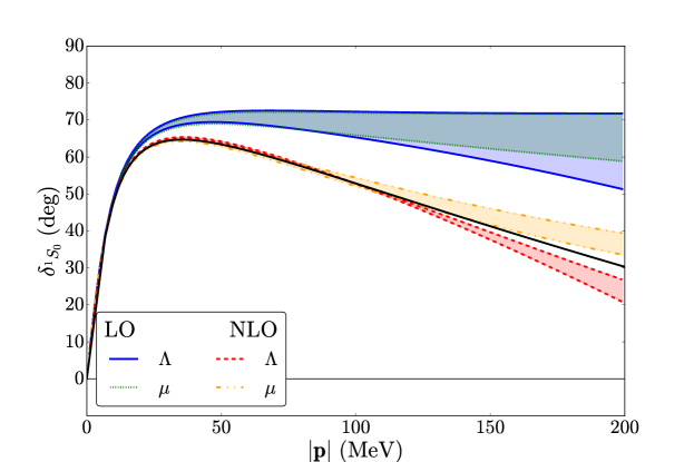
Figure 5: Phase shifts for $np$ scattering in the ${}^{1}S_{0}$ channel, computed in $\chi$EFT with a momentum space ($\Lambda$) cutoff and in dimensional regularization ($\mu$), as function of the center-of-mass momentum $|{\mathbf{p}}|$. The solid blue and dashed red lines denote the momentum-cutoff results at LO and NLO, respectively. The bands are obtained by varying $\Lambda$ between $2$ and $20$ fm^-1. The dotted green and dash-dotted orange lines are the LO and NLO results in dimensional regularization. The bands in the $\overline{\rm MS}$  scheme are obtained by varying the regulator of the intermediate scheme, as discussed in App. B, between $1/\lambda=0.05$ fm and $1/\lambda=0.7$ fm. $C$ is fit to the scattering length, and $C_{2}$ to the phase shift at $|{\mathbf{p}}|=30$ MeV. The black line shows the Nijmegen partial-wave analysis Stoks et al. (1993).

After this renormalization exercise we have a consistent description of the $N\!N$ system in the ${}^{1}S_{0}$ channel. We can now turn to the calculation of the $nn\rightarrow pp\,e^{-}e^{-}$ amplitude. In coordinate space, the LNV scattering amplitude is obtained by evaluating Eq. (61). In the momentum-space scheme, we use its analog,

$$\mathcal{A}_{\nu}=-2\pi^{2}\,\,{}^{-}\langle{}^{1}S_{0},\,p^{\prime}\,|V_{\nu}^{{}^{1}S_{0}}(p^{\prime},p)|{}^{1}S_{0},\,p\rangle^{+}$$ (73)

where

$$V^{{}^{1}S_{0}}_{\nu}(p^{\prime},p)=\int_{-1}^{1}\frac{dx}{(2\pi)^{2}}\,\frac{1}{p^{2}+p^{\prime\,2}-2pp^{\prime}x}\left[1+2g_{A}^{2}+\frac{g_{A}^{2}m_{\pi}^{2}}{\left(p^{2}+p^{\prime\,2}-2pp^{\prime}x+m_{\pi}^{2}\right)^{2}}\right]-\frac{g_{\nu}^{\rm NN}}{\pi^{2}}$$ (74)

is the partial-wave-projected neutrino potential and the $\pm$ superscripts indicates that we sandwich $V_{\nu}$ between scattered wavefunctions. We then calculate $\mathcal{A}_{\nu}$ via the explicit expression

$$\mathcal{A}_{\nu} = -2\pi^{2}\bigg{\{}V^{{}^{1}S_{0}}_{\nu}(p^{\prime},p)$$ (75)

$$+\int dp^{\prime\prime}\left[V^{{}^{1}S_{0}}_{\nu}(p^{\prime},p^{\prime\prime})\frac{m_{N}p^{\prime\prime\,2}}{p^{2}-p^{\prime\prime\,2}+i\varepsilon}T_{{}^{1}S_{0}}(p^{\prime\prime},p,E)+T_{{}^{1}S_{0}}(p^{\prime},p^{\prime\prime},E^{\prime})\frac{m_{N}p^{\prime\prime\,2}}{p^{\prime\,2}-p^{\prime\prime\,2}+i\varepsilon}V^{{}^{1}S_{0}}_{\nu}(p^{\prime\prime},p)\right]$$

$$+\int dp^{\prime\prime}\int dp^{\prime\prime\prime}\,T_{{}^{1}S_{0}}(p^{\prime},p^{\prime\prime},E^{\prime})\frac{m_{N}p^{\prime\prime\,2}}{p^{\prime\,2}-p^{\prime\prime\,2}+i\varepsilon}V^{{}^{1}S_{0}}_{\nu}(p^{\prime\prime},p^{\prime\prime\prime})\frac{m_{N}p^{\prime\prime\prime\,2}}{p^{2}-p^{\prime\prime\prime\,2}+i\varepsilon}T_{{}^{1}S_{0}}(p^{\prime\prime\prime},p,E)\bigg{\}}$$

or, in short-hand notation,

$$\mathcal{A}_{\nu}=-2\pi^{2}\left(V_{\nu}+V_{\nu}G_{0}T+TG_{0}V_{\nu}+TG_{0}V_{\nu}G_{0}T\right)\,.$$ (76)

The solution is graphically depicted in Figs. 3 and 4.

As illustrated in the right panel of Fig. 2, the amplitude $\mathcal{A}_{\nu}$ computed only with the long-range neutrino-exchange potential is cutoff dependent. The cutoff dependence is cured by introducing $g_{\nu}^{\rm NN}$ at LO. Figure 6 shows the values of the dimensionless coupling $\tilde{g}_{\nu}^{\rm NN}$, defined in Eq. (42), as a function of $R_{S}$, $\Lambda$, and the dimensional-regularization scale $\mu$. Because of the lack of data on $\Delta L=2$ processes, $\tilde{g}_{\nu}^{\rm NN}$ was determined here by requiring that the scattering amplitude at $|{\mathbf{p}}|=1$ MeV be equal to an arbitrarily chosen value,

$$\mathcal{A}_{\nu}(|{\mathbf{p}}|=1\,{\rm MeV},\,|{\mathbf{p}}^{\prime}|=38\,{\rm MeV})e^{-i(\delta_{{}^{1}S_{0}}(E)+\delta_{{}^{1}S_{0}}(E^{\prime}))}=-0.05\,{\rm MeV}^{-2}.$$ (77)

The values of $\tilde{g}_{\nu}^{\rm NN}$ obtained numerically with the $\Lambda$ and $R_{S}$ regulators are fitted with

$$\tilde{g}_{\nu}^{\rm NN}(\Lambda) = -12.0-2.2\,\ln(m_{\pi}/\Lambda)\,,\qquad\tilde{g}_{\nu}^{\rm NN}(R_{S})=-9.4-2.2\,\ln(m_{\pi}R_{S})\,,$$

$$\tilde{g}_{\nu}^{\rm NN}(\mu) = -7.9-2.1\,\ln(m_{\pi}/\mu)\,.$$ (78)

The coefficients of the logarithms in Eq. (78) are close to each other, and close to the dimensional-regularization expectation $(1+2g_{A}^{2})/2\simeq 2.1$. While intriguing, there is no proof that the coefficient of the logarithm should be universal, and counterexamples exist in the literature Beane et al. (2002).

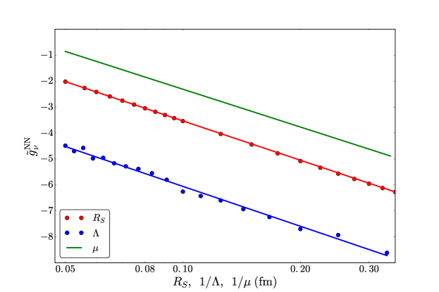
Figure 6: Dimensionless counterterm $\tilde{g}_{\nu}^{\rm NN}$ in $\chi$EFT as a function of the coordinate- and momentum-space cutoffs $R_{S}$ (red) and $\Lambda$ (blue), and of the dimensional-regularization scale $\mu$ (green). Red and blue points denote the results of numerical calculations, while the corresponding lines are logarithmic fits, as explained in the text. The counterterm is determined by imposing the (arbitrary) condition $\mathcal{A}_{\nu}\exp{(-i(\delta_{{}^{1}S_{0}}(E)+\delta_{{}^{1}S_{0}}(E^{\prime})))}=-0.05$ MeV^-2 at $|{\mathbf{p}}|=1$ MeV.

In Fig. 7 we show the renormalized $\mathcal{A}_{\nu}$ as a function of ${\mathbf{p}}$ in $\chi$EFT with momentum- and coordinate-space cutoffs, and in dimensional regularization. The cutoff bands are obtained by varying $\Lambda$ between $0.4$ and $2$ GeV, and $R_{S}$ between $0.05$ and $0.7$ fm. The dimensional-regularization band, by varying the regulator of the intermediate scheme introduced in App. B between $1/\lambda=0.05$ fm and $1/\lambda=0.7$ fm. Also shown is the outcome in ${/\pi}$EFT with dimensional regularization. In ${/\pi}$EFT the LO amplitude can be made $\mu$-independent, so that no band from scale variation appears. Of course, there is an uncertainty from missing higher-order corrections. All results are in excellent agreement. The regulator dependence is negligible at small momenta, and is small even at $|{\mathbf{p}}|=150$ MeV: about $15\%$ in the momentum-space scheme and smaller in the other schemes. This dependence is significantly reduced if we vary $\Lambda$ between $0.6$ and $2$ GeV, indicating that $0.4$ GeV might be too low compared to the breakdown scale.

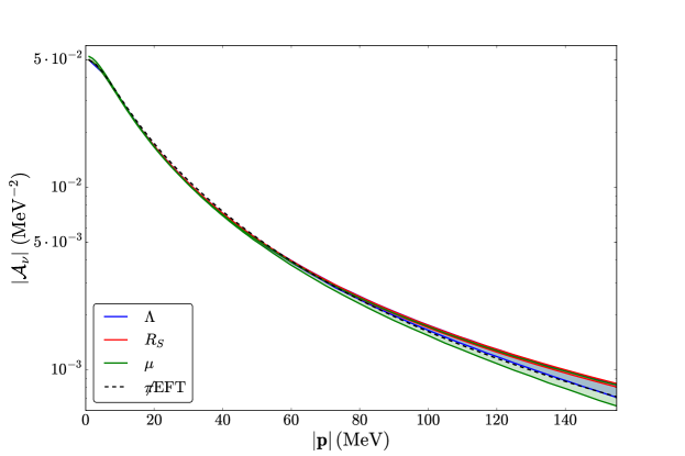
Figure 7: Magnitude of the LNV scattering amplitude $\mathcal{A}_{\nu}$ as a function of the neutron center-of-mass momentum $|{\mathbf{p}}|$ at LO. The red, blue, and green lines represent the results in $\chi$EFT with coordinate-space, momentum-space, and dimensional regularization, respectively, using $g_{\nu}^{\rm NN}$ from Fig. 6. The bands indicate residual regulator dependence, and are obtained by varying $R_{S}$ between $0.05$ and $0.7$ fm, $\Lambda$ between $2$ and $20$ fm^-1, and $1/\lambda$ between $0.05$ fm and $0.7$ fm. The dashed black line is the result in ${/\pi}$EFT with dimensional regularization. Since the ${/\pi}$EFT amplitude can be made exactly $\mu$-independent at this order, there is no band associated with the $\mu$ variations.

Note that treating pion exchange perturbatively Kaplan et al. (1998a, b), which might be sufficient at low energies Fleming et al. (2000); Kaplan (2019), does not avoid the presence of $g_{\nu}^{\rm NN}$ at LO, since in this case LO in the strong sector is identical to ${/\pi}$EFT. The conclusion is that after inclusion of $g_{\nu}^{\rm NN}$ the $nn\rightarrow pp\,e^{-}e^{-}$ amplitude is properly renormalized over the whole EFT momentum range.

V Neutrino potential in higher partial waves

In the previous sections we have demonstrated in various schemes the need to introduce an LO short-range counterterm for the $nn\rightarrow pp\,e^{-}e^{-}$ process for ${}^{1}S_{0}\rightarrow{}^{1}S_{0}$ transitions. We now investigate whether this problem also occurs for transitions involving higher partial waves. In ${/\pi}$EFT nucleons do not interact in these waves until higher orders, but in $\chi$EFT, as we discussed in Sec. III.2, there are renormalization issues already in the strong sector. We limit ourselves to two $P$-wave transitions ${}^{3}P_{0,1}\rightarrow{}^{3}P_{0,1}$, which allow us to examine the effects from the singular $N\!N$ tensor force generated by OPE while avoiding complications involved in the ${}^{3}P_{2}$-${}^{3}F_{2}$ coupled channel. In the ${}^{3}P_{1}$ channel this force is repulsive and one might expect no UV problems. However, in the ${}^{3}P_{0}$ channel it is attractive and similar problems as in the ${}^{1}S_{0}$ channel might occur. We also study the ${}^{1}D_{2}$ channel as representative of a singlet channel (where the OPE tensor force vanishes) with higher angular momentum $j$. In this section we stick to a single scheme, where we regulate the LS equation with a momentum cutoff.

We begin by describing the strong force in the $P$ and $D$ waves. We perform a partial-wave decomposition of the OPE potential (18) and obtain

$$\langle(l^{\prime}s^{\prime})j^{\prime}\,p^{\prime}|V_{\pi}|(ls)j\,p\rangle = 2\pi\sum_{f}\hat{f}^{\,3/2}\,(1\,1\,f\,;000)\sum_{\lambda_{1}+\lambda_{2}=f}\sqrt{\frac{\hat{f}!}{\hat{\lambda}_{1}!\hat{\lambda}_{2}!}}\;(p)^{\lambda_{2}}(-p^{\prime})^{\lambda_{1}}$$ (79)

$$\times\sum_{k}(-1)^{k}\hat{k}^{\,3/2}\,g_{k}^{f}(p,p^{\prime})\begin{pmatrix}k&k&0\\ \lambda_{1}&\lambda_{2}&f\\ l^{\prime}&l&f\end{pmatrix}\sqrt{\hat{\lambda}_{1}\hat{\lambda}_{2}}\;(k\,\lambda_{1}\,l^{\prime};000)\,(k\,\lambda_{2}\,l;000)$$

$$\times 6(-1)^{l}\sqrt{\hat{s}\hat{s^{\prime}}\hat{j}}\begin{pmatrix}l^{\prime}&\l&f\\ s^{\prime}&s&f\\ j^{\prime}&j&0\end{pmatrix}\begin{pmatrix}1/2&1/2&1\\ 1/2&1/2&1\\ s^{\prime}&s&f\end{pmatrix}\times(4t-3)\delta^{tt^{\prime}}\,,$$

where $t$ $(t^{\prime})$ is the total initial (final) isospin and $\hat{z}\equiv 2z+1$. We introduced the function

$$g^{f}_{k}(p,p^{\prime})=\int_{-1}^{1}dx\,P_{k}(x)\,V(q(x))\,q^{2-f}(x)\,,$$ (80)

in terms of the Legendre polynomials $P_{k}(x)$, $q^{2}(x)\equiv p^{2}+p^{\prime\,2}-2pp^{\prime}x$, and the function

$$V(q)=-\frac{g_{A}^{2}}{4F_{\pi}^{2}}\,\frac{1}{q^{2}+m_{\pi}^{2}}\,.$$ (81)

We solve the LS equation (68) for the potentials

$$V_{\{{}^{3}P_{0},{}^{3}P_{1},{}^{1}D_{2}\}}(p^{\prime},p)=\frac{1}{(2\pi)^{3}}\langle\{{}^{3}P_{0},{}^{3}P_{1},{}^{1}D_{2}\},\,p^{\prime}|V_{\pi}|\{{}^{3}P_{0},{}^{3}P_{1},{}^{1}D_{2}\},p\rangle\,,$$ (82)

where

$$\langle{}^{3}P_{0},\,p^{\prime}|V_{\pi}|{}^{3}P_{0},\,p\rangle = \frac{2\pi}{3}\left[g^{0}_{1}(p,p^{\prime})-4\left(p^{2}+p^{\prime\,2}\right)g^{2}_{1}(p,p^{\prime})+\frac{4}{3}\,pp^{\prime}\left(g^{2}_{2}(p,p^{\prime})+5g^{2}_{0}(p,p^{\prime})\right)\right]\,,$$

$$\langle{}^{3}P_{1},\,p^{\prime}|V_{\pi}|{}^{3}P_{1},\,p\rangle = \frac{2\pi}{3}\left[g^{0}_{1}(p,p^{\prime})+2\left(p^{2}+p^{\prime\,2}\right)g^{2}_{1}(p,p^{\prime})-\frac{2}{3}\,pp^{\prime}\left(g^{2}_{2}(p,p^{\prime})+5g^{2}_{0}(p,p^{\prime})\right)\right]\,,$$

$$\langle{}^{1}D_{2},\,p^{\prime}|V_{\pi}|{}^{1}D_{2},\,p\rangle = -2\pi\,g^{0}_{2}(p,p^{\prime})\,,$$ (83)

and extract the phase shifts from the solution of the T matrix.

As was found in Ref. Nogga et al. (2005), the pure OPE potential leads to cutoff-independent phase shifts in the (repulsive) ${}^{3}P_{1}$ and (mildly attractive) ${}^{1}D_{2}$ channels, but not in the (attractive) ${}^{3}P_{0}$ channel. This behavior is illustrated in the left-panel of Fig. 8, where the ${}^{1}D_{2}$ and ${}^{3}P_{1}$ phase shifts at $p=100$ MeV are flat, but the ${}^{3}P_{0}$ phase shift shows a limit-cycle-like behavior as a function of $\Lambda$. Following Ref. Nogga et al. (2005), we promote a counterterm to LO in the ${}^{3}P_{0}$ channel—the coupling $C_{{}^{3}P_{0}}$ in Eq. (20)—and fit it to the phase shift at a centre-of-mass energy $E_{CM}=25$ MeV. The resulting phase shifts are essentially cutoff independent as depicted in the left panel of Fig. 8. The phase shifts as a function of the relative momentum of the nucleons are depicted in the right panel of Fig. 8 and compared to the Nijmegen partial-wave analysis Stoks et al. (1993). After promoting the ${}^{3}P_{0}$ counterterm, the phase shifts in all three channels are well described at LO in $\chi$EFT.

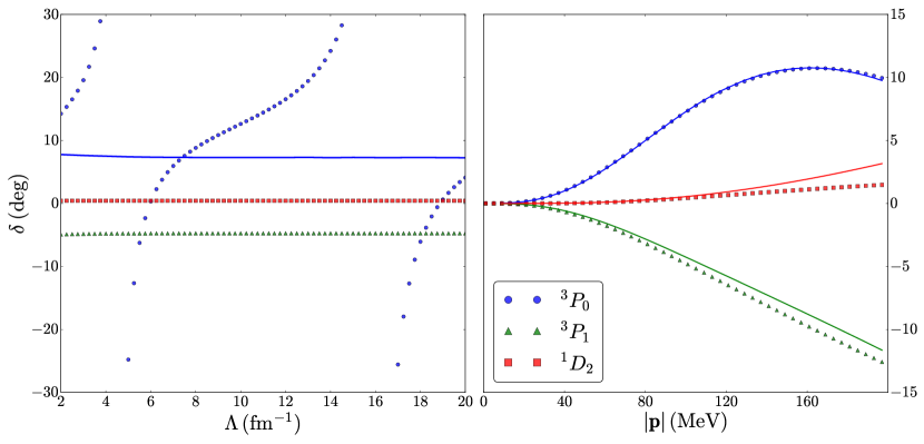
Figure 8: Left panel: Phase shifts in the ${}^{3}P_{0,1}$ and ${}^{1}D_{2}$ channels as a function of the momentum-space cutoff $\Lambda$. The green triangles, red squares, and blue circles denote respectively the ${}^{3}P_{1}$, ${}^{1}D_{2}$, and ${}^{3}P_{0}$ phase shifts from the OPE potential. The blue line is the ${}^{3}P_{0}$ phase shift with an additional counterterm. Right panel: the ${}^{1}D_{2}$ (red squares) ${}^{3}P_{1}$ (green triangles), and renormalized ${}^{3}P_{0}$ (blue circles) phase shifts as functions of the relative momentum of the nucleon pair $|{\mathbf{p}}|$, compared to the Nijmegen partial-wave analysis (solid lines) Stoks et al. (1993).

Having renormalized the strong interaction in the $P$-wave channels, we now turn to the $nn\rightarrow pp\,e^{-}e^{-}$ amplitude. We calculate Eq. (76) for ${}^{3}P_{0,1}\rightarrow{}^{3}P_{0,1}$ and ${}^{1}D_{2}\rightarrow^{1}D_{2}$ transitions. We only consider the long-range neutrino potential and do not include additional short-range LNV counterterms. We observe in the left panel of Fig. 9 that the resulting amplitudes are cutoff independent for the repulsive ${}^{3}P_{1}$ channel and the attractive ${}^{3}P_{0}$ channel, as well as the mildly attractive ${}^{1}D_{2}$ channel. Despite the attractive singular nature of the strong $N\!N$ interaction in the ${}^{3}P_{0}$ channel, the neutrino amplitude is UV finite. We conclude we do not need to promote additional counterterms to LO. In the right panel of Fig. 9 we plot the neutrino amplitude as a function of the neutron momentum and observe that the $P$-wave amplitudes are small compared to the $S$-wave amplitude. The $D$-wave amplitude becomes relatively important at higher values of $|{\mathbf{p}}|$, where the ${}^{1}S_{0}$ contribution has decreased significantly.

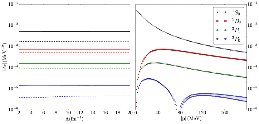
Figure 9: Left panel: absolute value of neutrino amplitude $\mathcal{A}_{\nu}$ for the ${}^{1}S_{0}$ (black), ${}^{1}D_{2}$ (red), ${}^{3}P_{1}$ (green), and ${}^{3}P_{0}$ (blue) channels as a function of momentum-space cutoff $\Lambda$. Solid (dashed) lines correspond to $|{\mathbf{p}}|=50$ MeV ($|{\mathbf{p}}|=100$ MeV). Right panel: absolute value of neutrino amplitude $\mathcal{A}_{\nu}$ in the ${}^{1}S_{0}$ (black stars), ${}^{1}D_{2}$ (red squares), ${}^{3}P_{1}$ (green triangles), and ${}^{3}P_{0}$ (blue dots) as functions of the neutron center-of-mass momentum $|{\mathbf{p}}|$. The bands (all except blue are nearly invisible) represent cutoff variation in the range $2$ to $20$ fm^-1.

VI The LNV scattering amplitude at next-to-leading order

In this section we study NLO corrections to the LNV amplitude $nn\rightarrow pp\,e^{-}e^{-}$. The main motivation to go to subleading order is the poor agreement between the observed phase shifts in the ${}^{1}S_{0}$ channel and the LO $\chi$EFT predictions, shown in Fig. 5. The agreement improves by including the contribution of the NLO operator $C_{2}$, and we want to study its impact on the $nn\rightarrow pp\,e^{-}e^{-}$ amplitude. In particular, we address the question whether a single counterterm $g_{\nu}^{\rm NN}$ is sufficient to renormalize the $\Delta L=2$ scattering amplitude up to NLO.

At NLO, ${/\pi}$EFT and $\chi$EFT contain a single momentum-dependent contact interaction in the ${}^{1}S_{0}$ channel, the $C_{2}$ defined in Eqs. (15) and (22). All other corrections in the singlet channels are expected to be of higher order. To study the strong and LNV scattering amplitudes in a generic scheme, it is convenient to split the non-derivative contact interactions $C$ and $g_{\nu}^{\rm NN}$ into LO and NLO pieces,

$$C=C^{(0)}+C^{(1)},\qquad g_{\nu}^{\rm NN}=g_{\nu}^{\rm NN\,(0)}+g_{\nu}^{\rm NN\,(1)},$$ (84)

with

$$C^{(0)}=\mathcal{O}\left(\frac{4\pi}{m_{N}Q}\right),~{}C^{(1)}=\mathcal{O}\left(\frac{4\pi}{m_{N}\Lambda}\right),\qquad g_{\nu}^{\rm NN\,(0)}=\mathcal{O}\left(\frac{1}{Q^{2}}\right),~{}g_{\nu}^{\rm NN\,(1)}=\mathcal{O}\left(\frac{1}{Q\Lambda}\right).$$ (85)

Here $\Lambda=\Lambda_{{/\pi}}$ in ${/\pi}$EFT and $\Lambda=\Lambda_{\chi}$ in $\chi$EFT, while $Q$ denotes the soft scale, that is, $Q\sim\aleph$ in ${/\pi}$EFT and $Q\sim m_{\pi}$ in $\chi$EFT. This splitting does not lead to new LECs; it simply ensures that the LO fitting conditions are not affected by NLO corrections. $C^{(1)}$ and $g_{\nu}^{\rm NN\,(1)}$ absorb power divergences induced by $C_{2}=O(4\pi/(m_{N}Q^{2}\Lambda))$ that appear both in ${/\pi}$EFT and $\chi$EFT when using a cutoff scheme. In $\chi$EFT, $C^{(1)}$ absorbs divergences induced by the pion-exchange potential. To simplify the notation, we will continue to drop the superscript $(0)$ from the LO counterterms.

The diagrams entering the LNV scattering amplitude at NLO are shown in the lower panels of Figs. 3 and 4. In the notation of Sec. IV.1, the NLO scattering amplitude takes the form

$$\mathcal{A}^{\rm NLO}_{\nu} = \mathcal{A}_{A}+\chi^{+}_{{\mathbf{p}}^{\prime}}({\mathbf{0}})\left(K_{E^{\prime}}+K^{(1)}_{E^{\prime}}\right)\mathcal{A}_{B}+\mathcal{\bar{A}}_{B}\left(K_{E}+K_{E}^{(1)}\right)\chi^{+}_{{\mathbf{p}}}({\mathbf{0}})$$ (86)

$$+\chi^{+}_{{\mathbf{p}}^{\prime}}({\mathbf{0}})\left(K_{E^{\prime}}+K^{(1)}_{E^{\prime}}\right)\left(\mathcal{A}_{C}+\frac{2g_{\nu}^{\rm NN}}{C^{2}}\right)\left(K_{E}+K_{E}^{(1)}\right)\chi^{+}_{{\mathbf{p}}}({\mathbf{0}})$$

$$+\chi^{+}_{{\mathbf{p}}^{\prime}}({\mathbf{0}})\,K_{E^{\prime}}\,\mathcal{A}^{(1)}_{B}+\mathcal{\bar{A}}^{(1)}_{B}\,K_{E}\,\chi^{+}_{{\mathbf{p}}}({\mathbf{0}})+\chi^{+}_{{\mathbf{p}}^{\prime}}({\mathbf{0}})\,K_{E^{\prime}}\,\mathcal{A}^{(1)}_{C}\,K_{E}\,\chi^{+}_{{\mathbf{p}}}({\mathbf{0}})\,,$$

where the superscript ${(1)}$ denotes NLO corrections, and terms quadratic in $K_{E,\,E^{\prime}}^{(1)}$ should be discarded. The first two lines in Eq. (86) subsume NLO corrections to the strong scattering amplitude, and yield a finite, regulator-independent result once the strong amplitude is renormalized. However, regulator dependence might appear in the remaining terms, shown in the third line.

To address this possible regulator dependence, we will also include the derivative operator $g_{2\nu}^{\rm NN}$, defined in Eq. (35). This operator only involves the $S$ wave, so when it is inserted into a bubble chain it will not cause any mixing with other partial waves. We therefore expect Bedaque and van Kolck (2002) $g_{2\nu}^{\rm NN}$ to be proportional to $C^{2}$ in the same way as $g_{\nu}^{\rm NN}$ Cirigliano et al. (2018b), and we define the rescaled coupling

$$\tilde{g}^{\rm NN}_{2\nu}=\left(\frac{4\pi}{m_{N}C}\right)^{2}g_{2\nu}^{\rm NN}$$ (87)

in analogy to Eq. (42). On the basis of the NDA Bedaque and van Kolck (2002), we expect the ratio of couplings to scale as

$$\frac{g_{2\nu}^{\rm NN}}{g_{\nu}^{\rm NN}}=\mathcal{O}\left(\frac{1}{\Lambda^{2}}\right),$$ (88)

implying that $g_{2\nu}^{\rm NN}$ contributes at N²LO. We will examine whether the renormalization of the full neutrino potential fulfills this expectation.

In ${/\pi}$EFT, the diagrams can be analytically resummed in any scheme where additional loops arising from insertions of contact interactions factorize. One example is the momentum scheme introduced in Eq. (54). In $\chi$EFT, because of the iteration of the pion-exchange potential, loop diagrams in general do not factorize, and we require a numerical solution. In dimensional regularization, however, the structure of the diagrams is simple enough that it is possible to give analytical expressions, which closely resemble those of ${/\pi}$EFT. We start by discussing the amplitude at NLO in ${/\pi}$EFT in Sec. VI.1. and extend the discussion to $\chi$EFT with dimensional and cutoff regularization in Secs. VI.2 and VI.3, respectively.

VI.1 Pionless EFT

In ${/\pi}$EFT, $K_{E}+K_{E}^{(1)}$ correspond to the full ${}^{1}S_{0}$ NLO scattering amplitude,

$$\left(K_{E}+K^{(1)}_{E}\right)_{{/\pi}}=\frac{1}{C^{-1}+I_{0}({\mathbf{p}})}\left[1+\left(\frac{C_{2}}{C^{2}}{\mathbf{p}}^{2}+\frac{C_{2}}{C}\delta I_{0}+\frac{C^{(1)}}{C^{2}}\right)\frac{1}{C^{-1}+I_{0}({\mathbf{p}})}\right],$$ (89)

where $I_{0}$ is defined in Eq. (43) and $\delta I_{0}$ is an integral that vanishes in dimensional regularization but is non-zero when using a momentum cutoff,

$$\delta I_{0}=-m_{N}\int\frac{d^{3}k}{(2\pi)^{3}}\exp\left[-2\frac{({\mathbf{k}}^{2})^{2}}{\Lambda^{4}}\right]\propto m_{N}\Lambda^{3}\,.$$ (90)

Its precise value is not important because the choice

$$C^{(1)}=-C_{2}\,C\,\delta I_{0}$$ (91)

exactly cancels its contribution. With this choice, the scattering length is not affected by NLO corrections, while $C_{2}$ is fixed by the effective range. Using Eq. (17) we obtain

$$\left(K_{E}+K^{(1)}_{E}\right)_{{/\pi}}=\frac{4\pi}{m_{N}}\frac{1}{1/a+i|{\mathbf{p}}|}\left(1+\frac{r_{0}{\mathbf{p}}^{2}}{2}\frac{1}{1/a+i|{\mathbf{p}}|}\right)\,,$$ (92)

which is regulator independent. Thanks to $\tilde{g}_{\nu}^{\rm NN}$, which compensates for the regulator dependence of ${\cal A}_{C}$, the first two lines of Eq. (86) are indeed independent of the regularization scheme.

The remaining corrections to the LNV amplitude in Eq. (86) are given by

$$\mathcal{A}_{B}^{(1)} = \frac{C_{2}}{2C}\,I_{1}({\mathbf{p}}^{\prime\,2})\,,\qquad\bar{\mathcal{A}}^{(1)}_{B}=\frac{C_{2}}{2C}\,I_{1}({\mathbf{p}}^{2})\,,$$ (93)

$$\mathcal{A}_{C}^{(1)} = \left(-\frac{4g_{\nu}^{\rm NN}}{C^{2}}\frac{C_{2}}{C}+\frac{2g_{2\nu}^{\rm NN}}{C^{2}}\right)\frac{{\mathbf{p}}^{2}+{\mathbf{p}}^{\prime\,2}}{2}+\frac{2g_{\nu}^{\rm NN\,(1)}}{C^{2}}+2\left(C_{2}\frac{g_{\nu}^{\rm NN}}{C^{2}}+\frac{g_{2\nu}^{\rm NN}}{C}\right)\delta I_{0}-\frac{C_{2}}{C}I_{2}({\mathbf{p}}^{2},{\mathbf{p}}^{\prime\,2}),\quad$$ (94)

where we used Eq. (91) and defined the cutoff-regularized integrals

$$I_{1}({\mathbf{p}}^{2}) = m_{N}\int\frac{d^{3}k}{(2\pi)^{3}}\frac{1+3g_{A}^{2}}{({\mathbf{p}}-{\mathbf{k}})^{2}}\,\exp\left[-\left(\frac{{\mathbf{k}}^{2}}{\Lambda^{2}}\right)^{2}\right]\,,$$

$$I_{2}({\mathbf{p}}^{2},{\mathbf{p}}^{\prime\,2}) = -\frac{m_{N}^{2}}{2}\int\frac{d^{3}k_{1}}{(2\pi)^{3}}\int\frac{d^{3}k_{2}}{(2\pi)^{3}}\frac{1+3g_{A}^{2}}{({\mathbf{k}}_{1}-{\mathbf{k}}_{2})^{2}}\frac{1}{{\mathbf{p}}^{2}-{\mathbf{k}}_{2}^{2}}\,\exp\left[-\left(\frac{{\mathbf{k}}_{1}^{2}}{\Lambda^{2}}\right)^{2}\right]\,\exp\left[-\left(\frac{{\mathbf{k}}_{2}^{2}}{\Lambda^{2}}\right)^{2}\right]$$ (95)

$$+({\mathbf{p}}\rightarrow{\mathbf{p}}^{\prime})\,.$$

In dimensional regularization these integrals vanish. There is, as a consequence, no scale dependence other than in the ${\mathbf{p}}^{2}+{\mathbf{p}}^{\prime\,2}$ term of $\mathcal{A}_{C}^{(1)}$, and we can take

$$g_{\nu}^{\rm NN\,(1)}=0\,.$$ (96)

Since in the absence of the derivative counterterm $g_{2\nu}^{\rm NN}$ the ${\mathbf{p}}^{2}+{\mathbf{p}}^{\prime\,2}$ term in Eq. (94) is $\mu$-dependent, the two-derivative operator in Eq. (35) is required to appear at NLO. It obeys the RGE

$$\frac{d}{d\ln\mu}\left(\tilde{g}^{\rm NN}_{2\nu}-2\eta\,C\,\tilde{g}_{\nu}^{\rm NN}\right)=0\,,$$ (97)

where we used Eq. (17) and introduced the dimensionless combination

$$\eta=\frac{m_{N}r_{0}}{8\pi}\,.$$ (98)

The solution of this RGE is

$$\tilde{g}^{\rm NN}_{2\nu}(\mu)=2\eta\,C(\mu)\,\tilde{g}_{\nu}^{\rm NN}(\mu)+\tilde{g}^{0}_{2\nu},$$ (99)

where $\tilde{g}^{0}_{2\nu}$ is an integration constant, and Eqs. (93) and (94) reduce to

$$\mathcal{A}_{B}^{(1)} = 0\,,\qquad\bar{\mathcal{A}}^{(1)}_{B}=0\,,$$ (100)

$$\mathcal{A}_{C}^{(1)} = \mathcal{A}^{(1)}_{C}=\left(\frac{m_{N}}{4\pi}\right)^{2}2\tilde{g}^{0}_{2\nu}\,\frac{{\mathbf{p}}^{2}+{\mathbf{p}}^{\prime\,2}}{2}\,,$$ (101)

which are independent of the renormalization scale. NDA rules modified to take into account S-wave enhancements Bedaque and van Kolck (2002) imply that

$$\tilde{g}^{0}_{2\nu}=\mathcal{O}\left(\frac{1}{\Lambda^{2}_{{/\pi}}}\right)\,,$$ (102)

so that Eq. (101) is actually an N²LO correction. So we find that in dimensional regularization with PDS scheme the coupling $g_{2\nu}^{\rm NN}$ involves an NLO piece fixed in terms of LO quantities by Eq. (97) and an N²LO piece parameterized by the constant $\tilde{g}^{0}_{2\nu}$, whose scaling is determined by NDA. This non-homogeneous scaling of $g_{2\nu}^{\rm NN}$ is analogous to the one of the four-derivative operator $C_{4}$ in the strong-interaction Lagrangian, which enters the $N\!N$ scattering amplitude with a fixed coefficient at N²LO, while a new LEC related to the shape parameter appears at N³LO Kaplan et al. (1998a); van Kolck (1999). As with an infinite number of other LECs, we cannot a priori exclude an enhancement of $\tilde{g}^{0}_{2\nu}$ over NDA, which could make it NLO or even LO, but currently we lack evidence for it. Equations (99) and (102) imply that the only NLO corrections to $\mathcal{A}_{\nu}$ come in through the strong scattering amplitude $T_{{}^{1}S_{0}}$.

We will now see that this argument is corroborated by a different choice of regularization. With a momentum cutoff, $I_{1}$ contains a momentum-independent linear divergence, while $I_{2}$ has a logarithmic divergence proportional to the energies in addition to a momentum-independent quadratic divergence:

$$I_{1}({\mathbf{p}}^{2})\propto m_{N}\Lambda\,,$$ (103)

$$I_{2}({\mathbf{p}}^{2},{\mathbf{p}}^{\prime\,2})\propto m_{N}^{2}\left(\Lambda^{2}+\kappa\frac{{\mathbf{p}}^{2}+{\mathbf{p}}^{\prime\,2}}{2}\ln\frac{\Lambda^{2}}{\Lambda_{0}^{2}}\right)\,,$$ (104)

where $\kappa$ is a dimensionless constant and $\Lambda_{0}$ is a constant with dimensions of momentum. We can thus write

$$I_{1}({\mathbf{p}}^{2})=I_{1}(0)+{\mathcal{O}}\left(\frac{m_{N}{\mathbf{p}}^{2}}{\Lambda}\right)\,,$$ (105)

$$I_{2}({\mathbf{p}}^{2},{\mathbf{p}}^{\prime\,2})=I_{2}(0,0)+\frac{{\mathbf{p}}^{2}+{\mathbf{p}}^{\prime 2}}{2}\left[\left(\frac{\partial}{\partial{\mathbf{p}}^{2}}+\frac{\partial}{\partial{\mathbf{p}}^{\prime 2}}\right)I_{2}({\mathbf{p}}^{2},{\mathbf{p}}^{\prime\,2})\right]_{{\mathbf{p}}^{2}={\mathbf{p}}^{\prime\,2}=0}+{\mathcal{O}}\left(\frac{m_{N}^{2}}{\Lambda^{2}}\left(\frac{{\mathbf{p}}^{2}+{\mathbf{p}}^{\prime\,2}}{2}\right)^{2}\right)\,.$$

In a cutoff scheme, Eq. (17) holds with $\mu\to c\Lambda$, the value of $c$ depending on the choice of regulating function. With $C\propto(m_{N}\Lambda)^{-1}$ and $C_{2}\propto(m_{N}\Lambda^{2})^{-1}$, we see that $\mathcal{A}_{B}^{(1)}$ is finite as $\Lambda\rightarrow\infty$. The regulator dependence in the momentum-independent terms of $\mathcal{A}_{C}^{(1)}$,

$$\frac{2g_{\nu}^{\rm NN\,(1)}}{C^{2}}+2\left(C_{2}\frac{g_{\nu}^{\rm NN}}{C^{2}}+\frac{g_{2\nu}^{\rm NN}}{C}\right)\delta I_{0}-\frac{C_{2}}{C}I_{2}(0,0)\,,$$ (107)

can be absorbed by a shift in the NLO LEC $g_{\nu}^{\rm NN\,(1)}$. The terms proportional to ${\mathbf{p}}^{2}+{\mathbf{p}}^{\prime\,2}$ converge as the cutoff is sent to infinity, albeit slowly,

$$\frac{{\mathbf{p}}^{2}+{\mathbf{p}}^{\prime\,2}}{2}\left\{-\frac{4C_{2}}{C}\frac{g_{\nu}^{\rm NN}}{C^{2}}-\frac{C_{2}}{C}\left[\left(\frac{\partial}{\partial{\mathbf{p}}^{2}}+\frac{\partial}{\partial{\mathbf{p}}^{\prime 2}}\right)I_{2}({\mathbf{p}}^{2},{\mathbf{p}}^{\prime\,2})\right]_{{\mathbf{p}}^{2}={\mathbf{p}}^{\prime\,2}=0}\right\}\propto\frac{{\mathbf{p}}^{2}+{\mathbf{p}}^{\prime\,2}}{2}\frac{\ln\Lambda}{\Lambda}\,.$$ (108)

Since higher powers of ${\mathbf{p}}^{2}+{\mathbf{p}}^{\prime\,2}$ converge as well, we conclude that in a cutoff scheme there is also no need to include an independent parameter at NLO. $g_{2\nu}^{\rm NN}$ can be included at this order with a fixed coefficient (as in dimensional regularization) as part of an “improved action” where cutoff artifacts scale more favorably as $1/\Lambda$ (instead of $\ln(\Lambda)/\Lambda$) and is thus of the same size as corrections that scale with the inverse of the breakdown scale.

In conclusion, the NLO analysis of $\mathcal{A}_{\nu}$ in both dimensional and cutoff regularizations shows that there appears no new independent LEC in the NLO neutrino potential. In dimensional regularization, $g_{2\nu}^{\rm NN}$ must be introduced to guarantee that $\mathcal{A}_{\nu}$ is scale independent, but its value is fixed by Eq. (99) in terms of $g_{\nu}^{\rm NN}$, the ${}^{1}S_{0}$ scattering length, and the ${}^{1}S_{0}$ effective range. In a cutoff scheme, Eq. (108) guarantees that for large $\Lambda$ the amplitude is correctly renormalized, after momentum-independent power divergences are absorbed by a redefinition of the LEC $g_{\nu}^{\rm NN}$. However, $g_{2\nu}^{\rm NN}$ with a cutoff dependence fixed by the same parameters as in dimensional regularization ensures that the error from $\Lambda$ at the breakdown scale is not unusually large.

VI.2 Chiral EFT with dimensional regularization

In $\chi$EFT, the NLO correction to the strong scattering amplitude encoded in

$$K_{E}^{(1)}=K^{2}_{E}\left[\frac{C^{(1)}}{C^{2}}+\frac{C_{2}}{C^{2}}\left({\mathbf{p}}^{2}-m_{N}V_{\pi}(0)\right)\right]$$ (109)

contains the additional contribution from the dimensionally regulated pion potential in coordinate space evaluated at the origin,

$$V_{\pi}(0) = -\frac{g_{A}^{2}}{4F_{\pi}^{2}}\int\frac{d^{d-1}k}{(2\pi)^{d-1}}\frac{m_{\pi}^{2}}{{\mathbf{k}}^{2}+m_{\pi}^{2}}=-\frac{g^{2}_{A}m_{\pi}^{2}}{16\pi F_{\pi}^{2}}\left(\mu-m_{\pi}\right)\,.$$ (110)

The $\mu$ dependence signals that the integral is linearly divergent in the PDS scheme. The $\mu$ independence of the strong scattering amplitude implies

$$\frac{d}{d\ln\mu}\left(\frac{C_{2}}{C^{2}}\right)=0\,,$$ (111)

but $C_{2}$ no longer has the simple expression in terms of the effective range given in Eq. (17) due to explicit pion-exchange contributions. Since $V_{\pi}(0)$ does not depend on the nucleon momenta, we can choose

$$C^{(1)}=m_{N}\,C_{2}\,V_{\pi}(0)$$ (112)

to cancel the linearly divergent terms. This choice ensures that NLO corrections do not change the scattering length.

As in ${/\pi}$EFT, the renormalization of the strong scattering amplitude implies that the first two lines in Eq. (86) are scale independent. The functions $\mathcal{A}^{(1)}_{B}$ and $\mathcal{A}^{(1)}_{C}$ are now given by

$$\mathcal{A}_{B}^{(1)} = \bar{\mathcal{A}}_{B}^{(1)}=0\,,$$ (113)

$$\mathcal{A}_{C}^{(1)} = \left(-\frac{4C_{2}}{C}\,\frac{g_{\nu}^{\rm NN}}{C^{2}}+\frac{2g_{2\nu}^{\rm NN}}{C^{2}}\right)\frac{{\mathbf{p}}^{2}+{\mathbf{p}}^{\prime 2}}{2}+\frac{2g^{\rm NN(1)}_{\nu}}{C^{2}}-2m_{N}V_{\pi}(0)\,\frac{g_{2\nu}^{\rm NN}}{C^{2}}+\frac{C_{2}}{C^{2}}\,m_{N}V_{\nu\,\rm L}(0)\,,$$ (114)

where

$$V_{\nu\,\rm L}(0)=\int\frac{d^{d-1}k}{(2\pi)^{d-1}}V^{{}^{1}S_{0}}_{\nu\,\rm L}({\mathbf{k}})=\frac{g_{A}^{2}m_{\pi}}{8\pi}\,$$ (115)

is the dimensionally regulated neutrino-exchange potential evaluated at the origin. $V_{\nu}(0)$ is finite in $\overline{\rm MS}$ and PDS, but would be linearly divergent in a cutoff scheme.

The subleading, momentum-independent $g^{\rm NN\,(1)}_{\nu}$ can be chosen to cancel the last three terms in Eq. (114). This choice implies that once $g_{\nu}^{\rm NN}$ is fitted to reproduce $\mathcal{A}_{\nu}$ at ${\mathbf{p}}=0$, its value is not affected by NLO corrections. Finally, the momentum dependent piece leads to the same RGE as in ${/\pi}$EFT,

$$\frac{d}{d\ln\mu}\left(\tilde{g}^{\rm NN}_{2\nu}-\frac{2C_{2}}{C}\tilde{g}_{\nu}^{\rm NN}\right)=0\,.$$ (116)

We conclude that also in $\chi$EFT $g_{2\nu}^{\rm NN}$ is completely determined at NLO by $g_{\nu}^{\rm NN}$ (in terms of $C_{2}$ and $C$), and new independent parameters appear only at N²LO or higher.

VI.3 Chiral EFT with cutoff regularization

Depending on the subtraction scheme, certain positive powers of a momentum cutoff have no analog in dimensional regularization. As a consequence, the need for a LEC at a given order might not be apparent in this regularization scheme, while it is in a cutoff scheme. We now check that the conclusion reached about $g_{2\nu}^{\rm NN}$ in $\chi$EFT does not depend on dimensional regularization. We repeat the analysis of Sec. VI.2 for the cutoff schemes introduced in Sec. IV.3.

In coordinate space, the amplitude at NLO is obtained by computing the integral (67) where now $\psi^{+}_{{\mathbf{p}}}({\mathbf{r}})=\psi^{+\,(0)}_{{\mathbf{p}}}({\mathbf{r}})+\psi^{+\,(1)}_{{\mathbf{p}}}({\mathbf{r}})$, with $\psi^{+\,(0)}_{{\mathbf{p}}}({\mathbf{r}})$ the LO wavefunction and

$$\psi^{+\,(1)}_{{\mathbf{p}}}({\mathbf{r}})=\frac{1}{E-H+i\varepsilon}\left[-\frac{C_{2}}{2}\left(\overleftarrow{\bm{\nabla}}^{2}\delta^{(3)}_{R_{S}}({\mathbf{r}})+\delta^{(3)}_{R_{S}}({\mathbf{r}})\overrightarrow{\bm{\nabla}}^{2}\right)+C^{(1)}\delta^{(3)}_{R_{S}}({\mathbf{r}})\right]\psi^{+\,(0)}_{{\mathbf{p}}}({\mathbf{r}})$$ (117)

the NLO correction, where $H$ is the LO Hamiltonian. To work consistently at NLO, we expand Eq. (67) and neglect terms quadratic in $\psi^{\pm(1)}_{{\mathbf{p}},{\mathbf{p}}^{\prime}}$. As in the momentum-space treatment below, $C_{2}$ and $C^{(1)}$ induce power-divergent corrections in the amplitude, which can be absorbed by introducing $g_{\nu}^{\rm NN\,(1)}$ in perturbation theory.

We also consider a momentum cutoff, where we start by solving the LS equation (68). Schematically, in first order in the NLO strong-interaction potential (23),

$$T^{(1)}=V^{(1)}+V^{(1)}G_{0}T+TG_{0}V^{(1)}+TG_{0}V^{(1)}G_{0}T\,,$$ (118)

where $T$ denotes the LO T matrix. This NLO correction to the T matrix induces a correction

$$S_{{}^{1}\!S_{0}}^{(1)}(E)=-i\pi m_{N}q_{0}\,T_{{}^{1}\!S_{0}}^{(1)}(q_{0},q_{0},E)$$ (119)

in the S matrix in the ${}^{1}\!S_{0}$ channel. We introduce the NLO phase shifts as

$$e^{2i(\delta_{{}^{1}\!S_{0}}(E)+\delta_{{}^{1}\!S_{0}}^{(1)}(E))}=S_{{}^{1}\!S_{0}}(E)+S_{{}^{1}\!S_{0}}^{(1)}(E)\qquad\rightarrow\qquad\delta_{{}^{1}\!S_{0}}^{(1)}(E)=\frac{1}{2i}\,\frac{S_{{}^{1}\!S_{0}}^{(1)}(E)}{S_{{}^{1}\!S_{0}}(E)}\,,$$ (120)

where $S_{{}^{1}\!S_{0}}(E)$ is the LO S matrix given by Eq. (71).

We now fit $C_{2}$ and $C^{(1)}$ by demanding that the scattering length, which was already correctly described at LO, be unaffected and, simultaneously, by fitting the ${}^{1}S_{0}$ phase shift at $|{\mathbf{p}}|=30$ MeV. More details of this procedure can be found in Ref. Long and Yang (2012). The resulting $np$ phase shifts with momentum and dimensional regularizations are shown in Fig. 5. Compared to LO, significantly better agreement with the Nijmegen partial-wave analysis Stoks et al. (1993) is obtained, but there is plenty of room for further improvement at higher orders. Results for the coordinate-space regulator are similar.

Having obtained the NLO T matrix, $T^{(1)}$, the calculation of the NLO neutrino amplitude is straightforward. Expanding Eq. (76) to first order

$$\mathcal{A}^{(1)}_{\nu} = -2\pi^{2}\left(V_{\nu}G_{0}T^{(1)}+T^{(1)}G_{0}V_{\nu}+T^{(1)}G_{0}V_{\nu}G_{0}T+TG_{0}V_{\nu}G_{0}T^{(1)}\right.$$ (121)

$$\left.+V^{(1)}_{\nu}+V^{(1)}_{\nu}G_{0}T+TG_{0}V^{(1)}_{\nu}+TG_{0}V^{(1)}_{\nu}G_{0}T\right)\,,$$

one sees that there are two types of corrections. The first type comes from the perturbative insertion of the NLO $T$ matrix. The contributions from $C_{2}$ and $C^{(1)}$ to $T^{(1)}$ induce power-divergent corrections to the amplitude. These can be absorbed by introducing $g_{\nu}^{\rm NN\,(1)}$, the momentum-independent NLO counterterm that corresponds to the NLO neutrino potential $V^{(1)}_{\nu}$. This piece then gives a second type of correction to the NLO amplitude.

The NLO counterterm $g_{\nu}^{\rm NN\,(1)}$ is fitted by demanding that $\mathcal{A}^{(1)}_{\nu}(|{\mathbf{p}}|=1\,\mathrm{MeV})=0$, such that the (arbitrary) LO fit condition at this energy employed in Sec. IV is not affected. We stress that $g_{\nu}^{\rm NN\,(1)}$ does not correspond to a new LEC but simply to a perturbative shift in the LO LEC. Only the sum $g_{\nu}^{\rm NN}+g_{\nu}^{\rm NN\,(1)}$ is relevant. In practice, $g_{\nu}^{\rm NN}+g_{\nu}^{\rm NN\,(1)}$, is quite different from $g_{\nu}^{\rm NN}$: even in the limited range of cutoffs commonly used in the literature, $R_{S}\sim 0.5-0.7$ fm, they differ by a factor of 2. While such variation is not unexpected in cutoff schemes, and has no effect on the observable $\mathcal{A}_{\nu}$, it highlights the importance of using consistent nuclear interactions in the extraction of $g_{\nu}^{\rm NN}$ and the calculation of $0\nu\beta\beta$ nuclear matrix elements.

The magnitude of the resulting $\Delta L=2$ scattering amplitude,

$$|\mathcal{A}_{\nu}|=|\mathcal{A}_{\nu}^{(0)}|+\frac{1}{|\mathcal{A}_{\nu}^{(0)}|}\textrm{Re}\left(\mathcal{A}_{\nu}^{(0)*}\mathcal{A}_{\nu}^{(1)}\right)+\dots\,,$$ (122)

is shown in Fig. 10 up to NLO for six values of $|{\mathbf{p}}|$ (namely $10,\,20,\,50,\,80,\,100,\,150$ MeV). The left panels correspond to the coordinate-space regulator and the right panels to the momentum-space regulator. Both schemes agree very well. LO results are the same as in Fig. 7 and given for comparison. NLO corrections to the amplitude are small and, more importantly, cutoff independent for sufficiently large cutoff. There is no numerical evidence for the need of an NLO counterterm. This observation is in agreement with the analysis in ${/\pi}$EFT with a hard cutoff, which showed that $g^{\rm NN}_{2\nu}$ is not needed for convergence as the cutoff increases. It is also consistent with the analysis in dimensional regularization in both ${/\pi}$EFT and $\chi$EFT, where it was concluded that no new LNV parameters appear until N²LO.

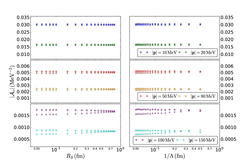
Figure 10: Magnitude of the LNV matrix element $\mathcal{A}_{\nu}$ at various values of the neutron center-of-mass momentum: $|{\mathbf{p}}|=10$, $20$, $50$, $80$, $100$, and $150$ MeV. Left and right panels show $\mathcal{A}_{\nu}$ as function of coordinate- and momentum-space regulators, respectively. Circles and triangles denote results at, respectively, LO and NLO. For the purpose of illustration, the LNV counterterm is determined by imposing the (arbitrary) condition $\left|\mathcal{A}_{\nu}\right|=0.05$ MeV^-2 at $|{\mathbf{p}}|=1$ MeV.

Of course, in the absence of data one cannot be sure $g^{\rm NN}_{2\nu}$ is not numerically large because of some fine tuning at small distances. Our arguments only show that there is no renormalization-group reason for it to be enhanced with respect to the estimate (88). In cutoff-regulated $\chi$EFT too, $g^{\rm NN}_{2\nu}$ could be included to accelerate convergence, but given the numerical nature of the calculation it could only be determined after the slow-converging results are obtained for one nucleus. Such an improved action would only be useful as input for calculations on a different nucleus.

VII The connection to charge-independence breaking

The analysis of Sec. IV shows that matrix elements of the long-range neutrino potential $V_{\nu\,{\rm L}}$, defined in Eq. (6), are ultraviolet divergent. The amplitude can be made independent of the UV regulator only by including at LO a short-range neutrino potential parametrized by $g_{\nu}^{\rm NN}$. While one can determine the dependence of $g^{\rm NN}_{\nu}$ on the renormalization scale $\mu$ or on the cutoff $\Lambda$ or $R_{S}$, knowledge of the finite piece of the LEC is necessary to make predictions for the $0\nu\beta\beta$ half-lives in terms of the effective neutrino Majorana mass $m_{\beta\beta}$. The argument in Sec. VI then shows that $g^{\rm NN}_{\nu}$ is the only LNV input needed up to NLO. It can in principle be extracted by matching the scattering amplitude for $nn\rightarrow pp\,e^{-}e^{-}$ in $\chi$EFT to LQCD. Such LQCD calculations are extremely challenging Cirigliano et al. (2019), but are beginning to be investigated. For instance, Ref. Feng et al. (2019) calculated the LEC associated to an N²LO LNV pion-electron coupling. In the absence of LQCD results, we discuss here how the size of LNV LECs, including $g_{\nu}^{\rm NN}$, can be estimated by studying their relation to analogous counterterms that are needed to describe isospin-breaking effects.

VII.1 The $I=2$ electromagnetic Lagrangian

In Sec. III.3 we derived the long-range neutrino potential, and discussed the form of short-range operators mediated by hard-neutrino exchange. We now explore the formal relation between LNV interactions and electromagnetic charge-independence breaking (CIB).

The starting point is the quark-level electromagnetic and weak Lagrangian

$$\mathcal{L}=\bar{q}_{L}\gamma^{\mu}\left(l_{\mu}+\hat{l}_{\mu}\right)q_{L}+\bar{q}_{R}\gamma^{\mu}\left(r_{\mu}+\hat{r}_{\mu}\right)q_{R}\,,$$ (123)

where $q$ denotes the quark doublet $q=(u\;d)^{T}$ and we defined

$$l_{\mu}=\frac{e}{2}A_{\mu}\,\tau^{3}-2\sqrt{2}\,G_{F}\left[V_{ud}\,\bar{e}_{L}\gamma_{\mu}\nu_{L}\,\tau^{+}+{\rm H.c.}\right]\,, \qquad\hat{l}_{\mu}=\frac{e}{6}A_{\mu}\,,$$ (124)

$$r_{\mu}=\frac{e}{2}A_{\mu}\,\tau^{3}\,, \qquad\hat{r}_{\mu}=\frac{e}{6}A_{\mu}\,.$$ (125)

We neglect weak neutral-current interactions that are not relevant to the present discussion. This Lagrangian gives rise to long-distance effects through couplings of photons and leptons to nucleons and pions. It induces the following one-body isovector amplitude

$$\mathcal{A}=\bar{N}\left[\frac{l_{\mu}+r_{\mu}}{2}J_{V}^{\mu}+\frac{l_{\mu}-r_{\mu}}{2}J_{A}^{\mu}\right]N,$$ (126)

where $J_{V}^{\mu}$ and $J_{A}^{\mu}$ are the vector and axial currents of Eq. (III.3). In addition, short-range operators are generated by the insertion of two currents connected by the exchange of hard photons (in the electromagnetic case) or neutrinos (in the case of $0\nu\beta\beta$). For $0\nu\beta\beta$ this mechanism gives rise to the $N\!N$ interactions of Sec. III.3 and additional $\pi N$ and $\pi\pi$ interactions, while electromagnetism (EM) induces very similar isospin $I=2$ interactions. This analogy between the two cases can be made precise by noticing that the insertion of two weak currents connected by a neutrino propagator with a single insertion of $m_{\beta\beta}$ leads to a massless (up to neutrino-mass corrections) boson propagator (in the Feynman gauge). The exchange of hard neutrinos therefore leads to identical contributions as photon exchange, up to an overall factor Cirigliano et al. (2018b): hard-neutrino exchange is multiplied by $8G_{F}^{2}V_{ud}^{2}m_{\beta\beta}\bar{e}_{L}e^{c}_{L}$ compared to the usual $e^{2}$ in the EM case. To elucidate this relation, we first construct the chiral Lagrangian in the $\pi\pi$ and $\pi N$ sectors for the LNV and EM cases, before discussing the short-range $N\!N$ interactions.

To construct operators that transform like two insertions of the weak and electromagnetic currents, we introduce the spurion fields for the left- and right-handed currents

$$\mathcal{Q}_{L} = u^{\dagger}Q_{L}u,\qquad\mathcal{Q}_{R}=uQ_{R}u^{\dagger}\,,$$ (127)

where $u^{2}=U=\exp(i\mbox{${\vec{\tau}}$}\cdot{\vec{\pi}}/F_{\pi})$ incorporates the pion fields. Under left- and right-handed chiral rotations $L$ and $R$, respectively, the meson $u$ and nucleon $N$ fields transform as $u\rightarrow LuK^{\dagger}=KuR^{\dagger}$ and $N\rightarrow KN$, where $K$ is an $SU(2)$ matrix that depends nonlinearly on the pion field. (For a review of chiral symmetry, see for example Ref. Bernard et al. (1995)). The spurions $Q_{L,R}$ transform like currents,

$$Q_{L} \rightarrow LQ_{L}L^{\dagger}\,,\qquad\,\,\,Q_{R}\rightarrow RQ_{R}R^{\dagger}\,,$$ (128)

$$\mathcal{Q}_{L} \rightarrow K\mathcal{Q}_{L}K^{\dagger}\,,\qquad\mathcal{Q}_{R}\rightarrow K\mathcal{Q}_{R}K^{\dagger}\,.$$ (129)

One then writes the most general Lagrangian involving $\mathcal{Q}_{L,R}$ that is invariant under chiral symmetry. The way weak currents break the symmetry is recovered by taking $Q\to Q^{\rm w}$ with

$$Q^{\rm w}_{L}=\tau^{+}\,,\qquad Q^{\rm w}_{R}=0\,.$$ (130)

In the EM case, $Q\to Q^{\rm em}$ with

$$Q^{\rm em}_{L}=Q^{\rm em}_{R}=\tau_{3}/2\,.$$ (131)

Because two insertions of $\mathcal{Q}^{\rm w}_{L}$ give rise to $I=2$ interactions in the $0\nu\beta\beta$ case, in the EM case we will investigate $I=2$ operators that induce CIB interactions.

In the mesonic sector, the only operator that can be constructed with two insertions of $Q_{L,R}$ and no derivatives is the $I=2$ interaction

$$\mathcal{L}^{\pi\pi}_{e^{2}}=Ze^{2}F_{\pi}^{4}\,\textrm{Tr}[\mathcal{Q}^{\rm em}_{L}\mathcal{Q}^{\rm em}_{R}]\,,$$ (132)

where, at LO in $\chi$PT, $Z$ is related to the pion-mass (squared) splitting by

$$Ze^{2}F_{\pi}^{2}=\frac{1}{2}\delta m^{2}_{\pi}=\frac{1}{2}\left(m_{\pi^{\pm}}^{2}-m_{\pi^{0}}^{2}\right).$$ (133)

There is no interaction of the type $Q_{L}^{2}$ that would lead to $|\Delta L|=2$. The first such interaction contains two chiral-covariant derivatives of the pion field,

$$u_{\mu}=-u^{\dagger}\left[i\partial_{\mu}+\left(l_{\mu}+\hat{l}_{\mu}\right)\right]u+u\left[i\partial_{\mu}+\left(r_{\mu}+\hat{r}_{\mu}\right)\right]u^{\dagger}\,,$$ (134)

and it is given by van Kolck (1993); Gasser et al. (2002); Cirigliano et al. (2018b)

$$\mathcal{L}^{\pi\pi}_{e^{2}} = -e^{2}F_{\pi}^{2}\,\kappa_{3}\left[\textrm{Tr}(\mathcal{Q}^{\rm em}_{L}u^{\mu})\,\textrm{Tr}(\mathcal{Q}^{\rm em}_{L}u_{\mu})-\frac{1}{3}\,\textrm{Tr}\left(\mathcal{Q}^{\rm em}_{L}\mathcal{Q}^{\rm em}_{L}\right)\,\textrm{Tr}\left(u^{\mu}u_{\mu}\right)+(L\rightarrow R)\right]\,,$$

$$\mathcal{L}^{\pi\pi}_{|\Delta L|=2} = \left(2\sqrt{2}\,G_{F}V_{ud}\right)^{2}m_{\beta\beta}\,\bar{e}_{L}C\bar{e}_{L}^{T}\,\frac{}{}\frac{5g_{\nu}^{\pi\pi}}{3(16\pi)^{2}}F_{\pi}^{2}$$ (135)

$$\times\left[\textrm{Tr}(\mathcal{Q}^{\rm w}_{L}u^{\mu})\,\textrm{Tr}(\mathcal{Q}^{\rm w}_{L}u_{\mu})-\frac{1}{3}\,\textrm{Tr}\left(\mathcal{Q}^{\rm w}_{L}\mathcal{Q}^{\rm w}_{L}\right)\,\textrm{Tr}\left(u^{\mu}u_{\mu}\right)\right]+{\rm H.c.}\,,$$

where we used the notation of Ref. Gasser et al. (2002) for the EM operator . $g_{\nu}^{\pi\pi}$ is a LEC of $\mathcal{O}(1)$, so that the operator in Eq. (135) contributes to the neutrino potential at N²LO, together with the pion-neutrino loops discussed in Ref. Cirigliano et al. (2018b). The factors of $e^{2}$ and $(2\sqrt{2}G_{F}V_{ud})^{2}m_{\beta\beta}\,\bar{e}_{L}C\bar{e}_{L}^{T}$ appear due to two insertions of EM and weak currents, respectively. This allows us to identify Cirigliano et al. (2018b)

$$g_{\nu}^{\pi\pi}=-\frac{3}{5}\left(16\pi\right)^{2}\kappa_{3}\,.$$ (136)

The model estimate of Ref. Ananthanarayan and Moussallam (2004) for $\kappa_{3}$ gives $g_{\nu}^{\pi\pi}(\mu=m_{\rho})=-7.6$, in agreement with a recent LQCD extraction that found $g_{\nu}^{\pi\pi}$ between $-12$ and $-8.5$ Feng et al. (2019); Feng .

In the single-nucleon sector, the lowest-order $|\Delta L|=2$ interaction involves one derivative. Focusing on terms with only $\mathcal{Q}^{\rm em}_{L}$ ($\mathcal{Q}^{\rm w}_{L}$) or $\mathcal{Q}^{\rm em}_{R}$, one can write van Kolck (1993); van Kolck et al. (1996); Gasser et al. (2002); Cirigliano et al. (2018b)

$$\mathcal{L}_{e^{2}}^{\pi N} = e^{2}F_{\pi}^{2}\,\frac{g_{4}+g_{5}}{4}\left[{\rm Tr}\left(u_{\mu}\mathcal{Q}^{\rm em}_{L}\right)\bar{N}S^{\mu}\mathcal{Q}^{\rm em}_{L}N-\frac{1}{3}\,\textrm{Tr}\left(\mathcal{Q}^{\rm em}_{L}\,\mathcal{Q}^{\rm em}_{L}\right)\bar{N}S^{\mu}u_{\mu}N+(L\rightarrow R)\right]\,,$$

$$\mathcal{L}_{|\Delta L|=2}^{\pi N} = \left(2\sqrt{2}G_{F}V_{ud}\right)^{2}m_{\beta\beta}\,\bar{e}_{L}C\bar{e}_{L}^{T}\,\frac{g_{A}g_{\nu}^{\pi N}}{4(4\pi)^{2}}$$ (137)

$$\times\left[{\rm Tr}\left(u_{\mu}\mathcal{Q}^{\rm w}_{L}\right)\bar{N}S^{\mu}\mathcal{Q}^{\rm w}_{L}N-\frac{1}{3}\,\textrm{Tr}\left(\mathcal{Q}^{\rm w}_{L}\mathcal{Q}^{\rm w}_{L}\right)\bar{N}S^{\mu}u_{\mu}N\right]+{\rm H.c.}\,,$$

where the LEC $g_{\nu}^{\pi N}=\mathcal{O}(1)$ is related to the EM LEC $g_{4}+g_{5}$ by Cirigliano et al. (2018b)

$$g_{\nu}^{\pi N}=\left(4\pi F_{\pi}\right)^{2}\,\frac{g_{4}+g_{5}}{g_{A}}\equiv-\frac{2}{g_{A}}\left(\frac{4\pi}{e}\right)^{2}\bar{\beta}_{10}\,.$$ (138)

The EM interactions induce CIB in the pion-nucleon couplings, but at the moment there exist no good estimates besides NDA. There is only a bound $\bar{\beta}_{10}=5(18)\cdot 10^{-3}$ van Kolck et al. (1996) extracted from the Nijmegen partial-wave analysis Stoks et al. (1993); van Kolck et al. (1998) of $N\!N$ scattering, which translates to $|g_{\nu}^{\pi N}|\hskip 1.99997pt\raisebox{2.15277pt}{$<$}\raisebox{-3.00003pt}{$\sim$}\hskip 1.99997pt61$. This introduces a source of uncertainty at N²LO in the chiral expansion of the neutrino potential.

We now come to the $N\!N$ sector, where the failure of Weinberg’s power counting requires the $|\Delta L|=2$ contact interaction in Eq. (33) at LO. The associated EM operators were constructed in Ref. Walzl et al. (2001). In the $m_{u,d}\rightarrow 0$ limit, there are only two rank-2 isospin operators with two insertions of $Q_{L,R}$ van Kolck (1993); Cirigliano et al. (2018b),

$$\mathcal{L}_{e^{2}}^{NN} = \frac{e^{2}}{4}\left\{\bar{N}\mathcal{Q}^{\rm em}_{L}N\,\bar{N}\!\left({\cal C}_{1}\mathcal{Q}^{\rm em}_{L}+{\cal C}_{2}\mathcal{Q}^{\rm em}_{R}\right)\!N-\frac{1}{6}\textrm{Tr}\left[\mathcal{Q}^{\rm em}_{L}\!\left({\cal C}_{1}\mathcal{Q}^{\rm em}_{L}+{\cal C}_{2}\mathcal{Q}^{\rm em}_{R}\right)\right]\bar{N}\mbox{${\vec{\tau}}$}N\cdot\bar{N}\mbox{${\vec{\tau}}$}N\right\}$$

$$+(L\rightarrow R)\,,$$

$$\mathcal{L}_{|\Delta L|=2}^{NN} = \left(2\sqrt{2}G_{F}V_{ud}\right)^{2}m_{\beta\beta}\bar{e}_{L}C\bar{e}_{L}^{T}\,\frac{g_{\nu}^{\rm NN}}{4}\left[\bar{N}\mathcal{Q}^{\rm w}_{L}N\,\bar{N}\mathcal{Q}^{\rm w}_{L}N-\frac{1}{6}\textrm{Tr}\left(\mathcal{Q}^{\rm w}_{L}\,\mathcal{Q}^{\rm w}_{L}\right)\bar{N}\mbox{${\vec{\tau}}$}N\cdot\bar{N}\mbox{${\vec{\tau}}$}N\right]$$ (139)

$$+{\rm H.c.}\,.$$

As before, the LECs $g_{\nu}^{\rm NN}$ and ${\cal C}_{1}$ are related, $g_{\nu}^{\rm NN}={\cal C}_{1}$. When expanded in powers of the pion field, the $|\Delta L|=2$ Lagrangian generates the contact interaction in Eq. (33). As we have seen, operators related to those in Eq. (139) but containing insertions of the quark masses are also needed at LO. The full set of such $N\!N$ operators with up to two mass insertions is constructed in App. A. In the isospin limit $m_{u}=m_{d}$, we can include quark-mass corrections by replacing ${\cal C}_{1}$ and ${\cal C}_{2}$ by the combinations

$$g_{\nu}^{\rm NN}={\cal C}_{1}=\sum_{n}c^{(1)}_{n}m_{\pi}^{2n}\,,\qquad{\cal C}_{2}=\sum_{n}c^{(2)}_{n}m_{\pi}^{2n}\,,$$ (140)

where $c_{n}^{(1,2)}$ are the couplings of the EM operators with $n$ mass insertions. The equality $g_{\nu}^{\rm NN}={\cal C}_{1}$ relies only on isospin symmetry and is not spoiled by insertions of the average quark mass.

If ${\cal C}_{1}$ and ${\cal C}_{2}$ can be fixed separately from CIB processes, then $g_{\nu}^{\rm NN}$ can be determined independently of LNV data. In Weinberg’s power counting, the LECs ${\cal C}_{1}$ and ${\cal C}_{2}$ scale as ${\cal C}_{1,2}=\mathcal{O}((4\pi F_{\pi})^{-2})$. In the following subsection we will show that renormalization requires ${\cal C}_{1,2}=\mathcal{O}(F_{\pi}^{-2})$, consistently with the enhancement of $g_{\nu}^{\rm NN}$. Unfortunately we cannot fix ${\cal C}_{1}$ and ${\cal C}_{2}$ separately at present, but we will discuss how CIB in the $N\!N$ system can be used to extract ${\cal C}_{1}+{\cal C}_{2}$.

VII.2 CIB in $N\!N$ scattering

We now determine the coefficient ${\cal C}_{1}+{\cal C}_{2}$ from $N\!N$ scattering data. By expanding the pion fields in the operators in Eq. (139), we see that ${\cal C}_{1}$ and ${\cal C}_{2}$ only differ at the multipion level. Any CIB observable that is not sensitive to multipion contributions therefore only constrains the sum ${\cal C}_{1}+{\cal C}_{2}$. In particular, $N\!N$ scattering data are not sufficient to determine ${\cal C}_{1}$, and thus $g_{\nu}^{\rm NN}$, separately as required for $0\nu\beta\beta$. Nevertheless, the analysis of CIB in $N\!N$ scattering does convincingly demonstrate the need for short-range operators to absorb divergences of Coulomb-like potentials acting in the ${}^{1}S_{0}$ channel. It provides a concrete data-driven example of the breakdown of Weinberg’s power counting. In addition, the extraction of ${\cal C}_{1}+{\cal C}_{2}$ will provide an estimate of the importance of the short-range neutrino potential by assuming $g_{\nu}^{\rm NN}\sim({\cal C}_{1}+{\cal C}_{2})/2$.

We start our discussion by demonstrating the need for CIB counterterms. Charge-independence breaking is evident in the difference between the ${}^{1}S_{0}$ $np$, $pp$, and $nn$ scattering lengths. In the $pp$ channel, Coulomb photon exchange is an LO effect at small center-of-mass momenta and the Coulomb potential must be iterated to all orders. We can define $a_{C}$ as the $pp$ scattering length after subtraction of the pure Coulomb contribution to $pp$ scattering. We will use the empirical determination of the scattering lengths Piarulli et al. (2015)

$$a_{np}=-23.7\pm 0.02\,\,\textrm{fm}\,,\qquad a_{nn}=-18.90\pm 0.40\,\,\textrm{fm}\,,\qquad a_{C}=-7.804\pm 0.005\,\,\textrm{fm}\,.$$ (141)

While we have subtracted long-range photon-exchange contributions, $a_{C}$ still contains short-range contributions from hard-photon exchange. These two types of contributions can be separated within specific models by defining a Coulomb-subtracted $pp$ scattering length Jackson and Blatt (1950), which is estimated to be $a_{pp}=-17.3\pm 0.4$ fm. From $a_{np}$, $a_{nn}$ and $a_{pp}$ we can construct the combination

$$a_{\rm CIB}=\frac{1}{2}\left(a_{pp}+a_{nn}\right)-a_{np}=5.6\pm 0.6\,\textrm{fm},$$ (142)

which demonstrates that CIB effects are sizable in the ${}^{1}S_{0}$ channel even after subtracting Coulomb contributions Miller et al. (1990). Since the separation between $a_{pp}$ and $a_{C}$ depends (mildly) on the model of the nuclear force, we will not use the Coulomb-subtracted scattering length and instead fit to $a_{C}$.

The most important pion-range CIB interaction stems from the pion-mass splitting, Eq. (132). Together with Coulomb-photon exchange, it gives rise through the diagrams in Fig. 11 to the long-range CIB potential van Kolck (1993); Friar and van Kolck (1999)

$$V_{\rm CIB}=\frac{e^{2}}{4}\left(\tau^{(1)}_{3}\tau^{(2)}_{3}-\frac{1}{3}\,\mbox{${\vec{\tau}}$}^{(1)}\cdot\mbox{${\vec{\tau}}$}^{(2)}\right)\frac{1}{{\mathbf{q}}^{2}}\left[1-\frac{g_{A}^{2}}{3}\frac{\delta m^{2}_{\pi}}{e^{2}F_{\pi}^{2}}\,\left(\mbox{\boldmath$\sigma$}^{(1)}\cdot\mbox{\boldmath$\sigma$}^{(2)}-S^{(12)}\right)\,\left(1-\frac{m_{\pi}^{2}}{{\mathbf{q}}^{2}+m_{\pi}^{2}}\right)^{2}\right]\,.$$ (143)

In the ${}^{1}S_{0}$ channel it reduces to

$$V^{{}^{1}S_{0}}_{\rm CIB}=\frac{e^{2}}{4}\left(\tau^{(1)}_{3}\tau^{(2)}_{3}-\frac{1}{3}\right)\frac{1}{{\mathbf{q}}^{2}}\left[1+g_{A}^{2}\frac{\delta m^{2}_{\pi}}{e^{2}F_{\pi}^{2}}\left(1-\frac{m_{\pi}^{2}}{{\mathbf{q}}^{2}+m_{\pi}^{2}}\right)^{2}\right]\,.$$ (144)

Since by NDA $\delta m^{2}_{\pi}={\mathcal{O}}(e^{2}F_{\pi}^{2})$, the pion-mass-splitting term is expected to contribute sizably to CIB for momenta $Q\sim m_{\pi}$.

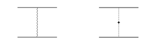
Figure 11: Long-range contributions to the CIB $N\!N$ potential. The wavy line represents a photon and the star denotes an insertion of the electromagnetic pion-mass splitting. Other symbols as in Fig. 1.

Equations (143) and (144) can be directly compared to, respectively, Eqs. (6) and (7). $V_{\rm CIB}$ has a very similar structure to the long-range neutrino potential $V_{\nu}$, with the difference that Eq. (6) contains contributions from the couplings of nucleons and pions to the weak axial current. In addition, there is no analog of the pion-mass-splitting term in $V_{\nu}$. The Coulombic nature of $V^{{}^{1}S_{0}}_{\rm CIB}$ at short distances implies that the same divergence we encountered in the LNV scattering amplitude $\mathcal{A}_{\nu}$ also affects CIB observables, requiring a CIB four-nucleon operator at LO in $e^{2}$.

The Coulombic nature of $V^{{}^{1}S_{0}}_{\rm CIB}$ also determines its importance relative to the LO strong interactions represented by $V^{{}^{1}S_{0}}_{\pi}$ in Eq. (11). For momenta $Q\sim m_{\pi}$, $V^{{}^{1}S_{0}}_{\rm CIB}/V^{{}^{1}S_{0}}_{\pi}\sim(eF_{\pi}/m_{\pi})^{2}\ll 1$ and $V^{{}^{1}S_{0}}_{\rm CIB}$ can be treated in perturbation theory. In this region, the argument of Sec. IV for the need of a counterterm goes through essentially unchanged for the CIB amplitude, if we replace the neutrino-exchange diagrams by Coulomb plus pion-mass-splitting OPE. The case of perturbative Coulomb in ${/\pi}$EFT has been examined in Ref. König et al. (2016). In contrast, at momenta $Q\hskip 1.99997pt\raisebox{2.15277pt}{$<$}\raisebox{-3.00003pt}{$\sim$}\hskip 1.99997pteF_{\pi}$ CIB is no longer a small correction since $V^{{}^{1}S_{0}}_{\rm CIB}/V^{{}^{1}S_{0}}_{\pi}\hskip 1.99997pt\raisebox{2.15277pt}{$>$}\raisebox{-3.00003pt}{$\sim$}\hskip 1.99997pt1$, but pion-mass-splitting OPE is $\hskip 1.99997pt\raisebox{2.15277pt}{$<$}\raisebox{-3.00003pt}{$\sim$}\hskip 1.99997pt(Q/m_{\pi})^{4}\ll 1$ compared to Coulomb. At even smaller momenta, $Q\hskip 1.99997pt\raisebox{2.15277pt}{$<$}\raisebox{-3.00003pt}{$\sim$}\hskip 1.99997pt\alpha_{\rm em}m_{N}\sim e^{2}F_{\pi}$, Coulomb-photon exchange is nonperturbative. The need for a counterterm for nonperturbative Coulomb in ${/\pi}$EFT was shown in Ref. Kong and Ravndal (2000). We generalize this argument now to $\chi$EFT including pion-mass splitting.

In order to interpolate smoothly between the three regions, we treat the CIB potential nonperturbatively. This is what is done in all chiral-potential calculations we are aware of. The iteration of the CIB potential does not affect the presence of a logarithmic divergence, which is due to diagrams where a single photon exchange or a single insertion of the pion-mass splitting is sandwiched between two short-range operators, analogous to the diagrams shown in the third row of Fig. 3. The iteration, however, affects the finite pieces of the counterterms by including corrections suppressed by powers of $e^{2}\sim 1/10$. Since the equality ${\cal C}_{1}=g_{\nu}^{\rm NN}$ is valid at LO in $e^{2}$, we expect the counterterms extracted from $N\!N$ scattering to be a good representation of the LNV counterterms up to $10\%$ corrections. In summary, we replace the long-range potential $V_{\pi}$ in Eq. (38) by different potentials in the $pp$, $nn$, and $np$ channels,

$$V_{pp}=V_{\pi}(m_{\pi^{0}})+\frac{e^{2}}{4\pi r},\qquad V_{nn}=V_{\pi}(m_{\pi^{0}})\,,\qquad V_{np}=2V_{\pi}(m_{\pi^{\pm}})-V_{\pi}(m_{\pi^{0}}),$$ (145)

with $m_{\pi^{\pm}}=139.57$ MeV and $m_{\pi^{0}}=134.98$ MeV.

In Weinberg’s power counting, the contact interaction $C$ is charge independent at LO. As discussed in Sec. VII.1, charge dependence only enters at $\mathcal{O}(e^{2}/(4\pi)^{2})$, which is suppressed by $(4\pi)^{-2}$ with respect to the terms in Eq. (145). This implies that once $C$ is determined in one isospin channel, for example $np$, the phase shifts in the remaining channels, $pp$ and $nn$, should be independent of the regulator. We test this prediction of Weinberg’s power counting in Fig. 12. We determine $C$ by fitting to $a_{np}$ in the $np$ channel and define the resulting value as $C_{np}$. We then calculate $a_{C}$ and $a_{nn}$ using the long-range potentials in Eq. (145) combined with the short-range interaction with LEC $C_{np}$. Figure 12 shows that $a_{C}$ and $a_{nn}$ have a strong dependence on the cutoff $R_{S}$, and for no $R_{S}$ in the plotted range there is agreement between the calculated and the measured values. As was the case for $0\nu\beta\beta$ decay, our calculations explicitly demonstrate that Weinberg’s power counting is inadequate for Coulomb-like potentials in the ${}^{1}S_{0}$ channel.

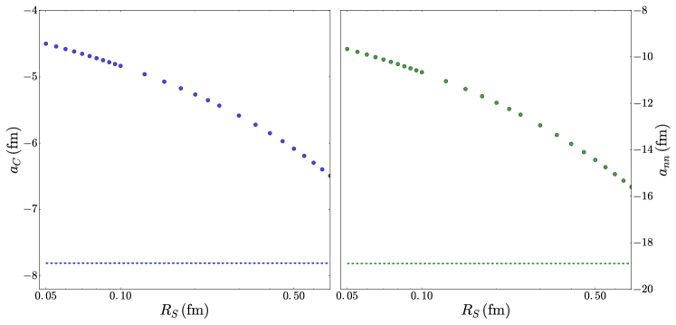
Figure 12: Proton-proton scattering length $a_{C}$ (left panel) and neutron-neutron scattering length $a_{nn}$ (right panel), as a function of the coordinate-space cutoff $R_{S}$. The points are computed with the long-range potentials $V_{pp}$ and $V_{nn}$ defined in Eq. (145), and with a charge-independent short-range potential with LEC $C=C_{np}$ fitted to the $np$ scattering length in the ${}^{1}S_{0}$ channel, $a_{np}$. The dashed lines indicate the experimental values of $a_{C}$ and $a_{nn}$.

The regulator dependence can be removed by introducing isospin-breaking counterterms $C_{np}$, $C_{nn}$, and $C_{pp}$. This amounts to including short-range charge-symmetry breaking (CSB) as well as CIB. According to NDA, OPE with a CSB pion-nucleon coupling van Kolck (1993); van Kolck et al. (1996); Friar et al. (2003) contributes at the same order as short-range CSB. The value of the CSB pion-nucleon coupling is unknown van Kolck et al. (1996, 1998), but its inclusion would not affect the conclusions drawn below that short-range CSB is enhanced over NDA, just as short-range CIB. For simplicity we do not include CSB OPE. We determine $C_{np}$, $C_{nn}$, and $C_{pp}$ by reproducing the observed scattering lengths in Eq. (141). We then extract the CIB combination

$$\frac{\mathcal{C}_{1}+\mathcal{C}_{2}}{2}\equiv\left(\frac{m_{N}C}{4\pi}\right)^{2}\frac{\tilde{\cal C}_{1}+\tilde{\cal C}_{2}}{2}=\frac{1}{e^{2}}\left(C_{np}-\frac{C_{nn}+C_{pp}}{2}\right)\,,$$ (146)

with $C=(C_{np}+C_{nn}+C_{pp})/3$. At small $R_{S}$, the dimensionless sum $\tilde{\cal C}_{1}+\tilde{\cal C}_{2}$ shows the expected logarithmic behavior,

$$\frac{\tilde{\cal C}_{1}+\tilde{\cal C}_{2}}{2}\simeq 0.4-1.95\,\ln(m_{\pi}R_{S})\,.$$ (147)

The fit in Eq. (147) is accurate up to $R_{S}\sim 0.3$ fm at which point power corrections become important. Note that for the values of $R_{S}$ commonly used in the literature, $0.5-0.8$ fm, the numerical value of $F_{\pi}^{2}({\cal C}_{1}+{\cal C}_{2})$ is in the range $0.15-0.2$, much larger than the $(4\pi)^{-2}$ predicted by Weinberg’s power counting.

The logarithmic divergence induced by the long-range potential $V_{\rm CIB}$ can be seen explicitly using the $\overline{\textrm{MS}}$ scheme. The analysis follows that in Sec. IV.1. The RGEs for $C_{np}$, $C_{pp}$ and $C_{nn}$ are modified by the isospin-breaking interactions:

$$\frac{d}{d\ln\mu}C_{pp}^{-1} = \left(\frac{m_{N}}{4\pi}\right)^{2}\left(e^{2}-\frac{g_{A}^{2}m_{\pi^{0}}^{2}}{4F_{\pi}^{2}}\right)\,,$$

$$\frac{d}{d\ln\mu}C_{np}^{-1} = \left(\frac{m_{N}}{4\pi}\right)^{2}\frac{g_{A}^{2}(m_{\pi^{0}}^{2}-2m_{\pi^{\pm}}^{2})}{4F_{\pi}^{2}}\,,$$

$$\frac{d}{d\ln\mu}C_{nn}^{-1} = -\left(\frac{m_{N}}{4\pi}\right)^{2}\frac{g_{A}^{2}m_{\pi^{0}}^{2}}{4F_{\pi}^{2}}\,,$$ (148)

which are solved to reproduce the scattering lengths in Eq. (141). The resulting phase shifts are shown in Fig. 13. Since we iterated the Coulomb potential in the $pp$ channel, we get a good description of the phase shifts at small momentum. For simplicity, we also iterated the pion-mass splitting by considering the physical pion masses in Eq. (145). In agreement with the expectation from NDA, isospin-breaking effects are relatively small at momenta comparable to the pion mass.

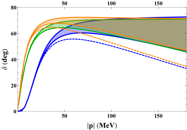
Figure 13: Phase shifts for the different isospin components in the ${}^{1}S_{0}$ channel as function of the center-of-mass momentum $|{\mathbf{p}}|$. Orange, blue, and green bands represent an $\overline{\rm MS}$ calculation of $np$, $pp$, and $nn$ scattering, respectively, where the regulator of the intermediate scheme, as discussed in App. B, is varied between $1/\lambda=0.05$ fm and $1/\lambda=0.7$ fm. The red and blue dashed lines show the Nijmegen partial-wave analysis for $np$ and $pp$ phase shifts, respectively Stoks et al. (1993).

The RGEs in Eq. (148) imply

$$\frac{d}{d\ln\mu}\tilde{\cal C}_{1} = \frac{1}{2}\left(1+2g_{A}^{2}\right)\simeq 2.1\,,$$ (149)

$$\frac{d}{d\ln\mu}\tilde{\cal C}_{2} = \frac{1}{2}\left(1-2g_{A}^{2}+2g_{A}^{2}\,\frac{\delta m^{2}_{\pi}}{e^{2}F_{\pi}^{2}}\right)\simeq 1.5\,.$$ (150)

Equation (149) agrees with Eq. (57), as it should. Using the fit values for $C_{nn,np,pp}$, we obtain

$$\frac{\tilde{\cal C}_{1}+\tilde{\cal C}_{2}}{2}\simeq 2.5-1.8\,\ln(m_{\pi}/\mu).$$ (151)

As for the $nn\rightarrow pp\,e^{-}e^{-}$ case, Eq. (78), the coefficient of the logarithms in $\overline{\textrm{MS}}$ and $R_{S}$ schemes agree at the 10% level. The coefficients of the logarithms in $(\tilde{\cal C}_{1}+\tilde{\cal C}_{2})/2$ and $\tilde{g}_{\nu}^{\rm NN}$ are numerically similar, while $\tilde{\cal C}_{1}-\tilde{\cal C}_{2}$ runs more slowly. This appears to be consequence of the numerical accident $\delta m^{2}_{\pi}\approx 2e^{2}F_{\pi}^{2}$, for which we are not aware of an underlying physical reason.

Finally, we comment on the possibility of using a similar analysis for the two-derivative short-range $0\nu\beta\beta$ operator. In Sect. VI we argued, based on a combination of renormalization-group arguments and NDA, that we expect a new LEC only to enter at N²LO in both pionless and chiral EFT. Focusing for simplicity on pionless EFT, we are concerned whether we can confirm the size of the LEC $\tilde{g}^{0}_{2\nu}$ in Eq. (102). This LEC is connected to the CIB combination of ${}^{1}S_{0}$ effective ranges Kong and Ravndal (1999, 2000)

$$(r_{0})_{\rm CIB}=\frac{(r_{0})_{pp}+(r_{0})_{nn}-2(r_{0})_{np}}{2}\sim e^{2}\frac{m_{N}}{4\pi}\tilde{g}^{0}_{2\nu}\,.$$ (152)

Using the scaling in Eq. (102), we obtain ${(r_{0})_{\rm CIB}}/{r_{0}}=\mathcal{O}(e^{2})$. This scaling agrees with NN scattering data that give Piarulli et al. (2015) $(r_{0})_{\rm CIB}/{r_{0}}\in[-0.04,0.06]$. An NLO scaling of $\tilde{g}^{0}_{2\nu}$ would predict much larger CIB corrections, ${(r_{0})_{\rm CIB}}/{r_{0}}=\mathcal{O}(e^{2}\Lambda_{{/\pi}}/\aleph)$, which are not supported by data.

VII.3 Impact on the two-body LNV amplitude

We can use the value of ${\cal C}_{1}+{\cal C}_{2}$ to estimate the numerical impact of the short-range component of the neutrino potential on $\mathcal{A}_{\nu}$. Since $N\!N$ scattering alone does not allow one to isolate ${\cal C}_{1}$, and thus the contribution to $0\nu\beta\beta$, we will first assume that $\tilde{\cal C}_{1}(\bar{R}_{S})=\tilde{\cal C}_{2}(\bar{R}_{S})$ at a given scale $\bar{R}_{S}$. Since ${\cal C}_{1}$ and ${\cal C}_{2}$ have different runnings, the renormalization point at which this choice is made influences the value of the amplitude. We assess this dependence by varying $\bar{R}_{S}$ in a wide range, between 0.05 and 0.7 fm. The corresponding results for $\mathcal{A}_{\nu}$ are shown in Table 1. With the suffixes L and S we denote the matrix elements of the long- and short-range neutrino potentials defined in Eqs. (6) and (36) (with $g_{2\nu}^{\rm NN}$ set to zero) respectively. We observe for $nn\rightarrow pp$ transitions, where the initial and final states have the same total isospin, a reduction of the total amplitude by 10-30% due to inclusion of the short-range potential.

$\bar{R}_{S}$ (fm)	$(\mathcal{A}_{\nu})_{\rm L}$ (MeV-2)	$(\mathcal{A}_{\nu})_{\rm S}$ (MeV-2)	$\mathcal{A}_{\nu}$ (MeV-2)
0.05	0.046	$-0.014$	0.032
0.1	0.043	$-0.012$	0.031
0.3	0.037	$-0.007$	0.030
0.7	0.032	$-0.00$4	0.028

Table 1: $nn\rightarrow pp\,e^{-}e^{-}$ scattering amplitude $\mathcal{A}_{\nu}$, divided by the factor $-\exp(i(\delta_{{}^{1}S_{0}}(E)+\delta_{{}^{1}S_{0}}(E^{\prime})))$, evaluated at $|{\mathbf{p}}|=$ 1 MeV and $|{\mathbf{p}}^{\prime}|=38$ MeV for selected values of the coordinate-space cutoff $\bar{R}_{S}$ where ${\cal C}_{1}(\bar{R}_{S})$ is assumed equal to ${\cal C}_{2}(\bar{R}_{S})$. The suffixes L and S label the matrix elements of the long- and short-range components of the neutrino potential.

While significant, the influence of the short-range potential is somewhat smaller than the $\mathcal{O}(1)$ expectation. This smallness can be understood by examining the matrix-element density $C(r)$ defined as

$$C_{\rm L,S}(r)=\int d^{3}{\mathbf{r}}^{\prime}\,\psi_{{\mathbf{p}}^{\prime}}^{-}({\mathbf{r}}^{\prime})^{*}\,V_{\nu\,\rm L,\,S}({\mathbf{r}}^{\prime})\,\delta(r-r^{\prime})\,\psi^{+}_{{\mathbf{p}}}({\mathbf{r}}^{\prime}).$$ (153)

We see in Fig. 14 that the long-range matrix element $C_{\rm L}(r)$ has support over a wide range of $r$.In contrast, $C_{\rm S}(r)$ is essentially zero for $r\hskip 1.99997pt\raisebox{2.15277pt}{$>$}\raisebox{-3.00003pt}{$\sim$}\hskip 1.99997pt1$ fm. Only for the smaller cutoff values does the short-range component become sufficiently large to partially compensate for the smaller range. Therefore, even if formally LO, the impact of $g_{\nu}^{\rm NN}$ is somewhat diluted. We will see in Sec. VIII that this is not the case for transitions in which the nuclear isospin changes by two units, which is the case for all nuclei of experimental interest.

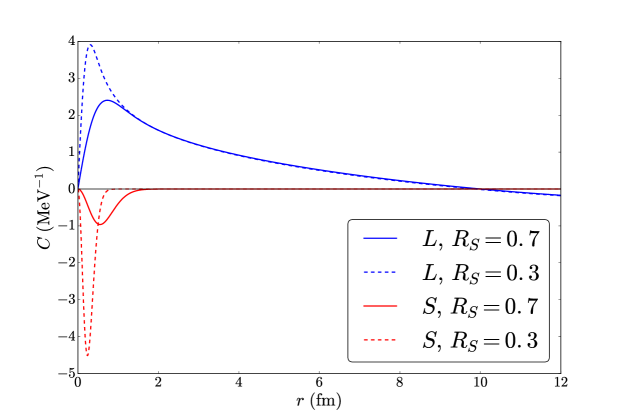
Figure 14: Matrix-element densities for the $nn\to ppe^{-}e^{-}$ transition as a function of the radial coordinate. Curves are shown for the long- (blue) and short-range (red) components of the $0\nu\beta\beta$ transition operator for two choices of the cutoff $R_{S}$, 0.7 (solid) and 0.3 (dashed) fm.

We stress that the choice ${\cal C}_{1}={\cal C}_{2}$ was made for illustration purposes only, and other choices can be made. This arbitrariness leads to an uncontrolled theoretical uncertainty. We can illustrate the effect of varying the assumption ${\cal C}_{1}={\cal C}_{2}$, by considering the more general situation ${\cal C}_{2}=\alpha{\cal C}_{1}$, or, equivalently,

$$\tilde{g}_{\nu}^{\rm NN}(\mu_{0})=\kappa\frac{\tilde{\cal C}_{1}(\mu_{0})+\tilde{\cal C}_{2}(\mu_{0})}{2},$$ (154)

with $\kappa=2/(1+\alpha)$ and $\mu_{0}$ the (arbitrary) scale where Eq. (154) holds. We show the result of varying $\kappa$ between $-1$ and $2$ in Fig. 15. The point $\kappa=0$ corresponds to no counterterm in the neutrino potential, while $\kappa=2$ to the situation in which ${\cal C}_{2}=0$ and all CIB arises from ${\cal C}_{1}$. The red bands are obtained by changing the renormalization point $\mu_{0}$ at which the choice in Eq. (154) is made. Figure 15 highlights that CIB in $N\!N$ scattering, while providing strong evidence for the existence of a counterterm in $0\nu\beta\beta$, unfortunately does not allow us to draw robust quantitative conclusions about its impact in the magnitude of renormalized amplitude. It does demonstrate that a better understanding of the short-range contributions is crucial, since reasonable $\mathcal{O}(1)$ choices for $\kappa$ lead to variations of the $nn\rightarrow pp\,e^{-}e^{-}$ amplitude of roughly an order of magnitude. This uncertainty must be reduced to reliably extract the effective Majorana neutrino mass from $0\nu\beta\beta$ decay experiments.

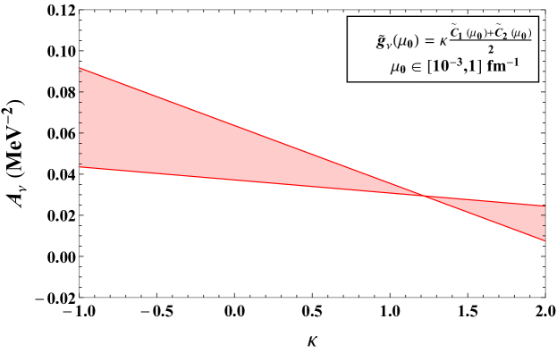
Figure 15: Dependence of the sum of the short- and long-range $nn\rightarrow pp\,e^{-}e^{-}$ amplitudes at ${\mathbf{p}}=1$ MeV, on the parameter $\kappa$ that parametrizes the relation between $\tilde{g}_{\nu}$ and the CIB counterterms $\tilde{\cal C}_{1}+\tilde{\cal C}_{2}$ at a given scale $\mu_{0}$. The bands are obtained by varying $\mu_{0}$ between $10^{-3}$ and $1$ fm^-1.

VIII Phenomenological implications

In the previous sections, we have demonstrated the need to include a counterterm to absorb divergences induced by the long-range neutrino potential: in coordinate space,

$$V_{\nu\,\rm S}=-2g_{\nu}^{\rm NN}\,\tau^{(1)+}\tau^{(2)+}\delta^{(3)}_{R_{S}}({\bf r})\ ,$$ (155)

with $\delta^{(3)}_{R_{S}}({\bf r})$ a regularization of the delta function such as Eq. (66). The value of $g_{\nu}^{\rm NN}$ depends on nonperturbative QCD dynamics, and, lacking a measurement of the $nn\rightarrow pp\,e^{-}e^{-}$ cross section, could be determined by matching to LQCD calculations of LNV processes. In Sec. VII, we have established a relation between the contact interactions appearing in the LNV and in the EM Lagrangian, which leads to $g_{\nu}^{\rm NN}=\mathcal{C}_{1}$. The electromagnetic counterpart of the LNV contact potential $V_{\nu\,\rm S}$,

$$V_{\rm CIB,\,\rm S}=-\frac{e^{2}}{6}\frac{{\cal C}_{1}+{\cal C}_{2}}{2}\,T^{(12)}\,\delta^{(3)}_{R_{S}}({\bf r})\ ,$$ (156)

where the isotensor operator reads $T^{(12)}=3\,\tau^{(1)}_{3}\tau^{(2)}_{3}-\mbox{${\vec{\tau}}$}^{(1)}\cdot\mbox{${\vec{\tau}}$}^{(2)}$, is included in all high-quality phenomenological Machleidt (2001); Wiringa et al. (1995) and chiral potentials Machleidt and Entem (2011); Epelbaum et al. (2015); Piarulli et al. (2015); Ekström et al. (2015); Piarulli et al. (2016); Reinert et al. (2018), as it was recognized that just including the Coulomb interaction and the pion-mass splitting does not reproduce the CIB in the $N\!N$ scattering lengths. In the previous section we have seen that renormalization of the amplitude with Coulomb-photon exchange in fact demands the presence of this short-range interaction. In this section, we extract the value of $({\cal C}_{1}+{\cal C}_{2})/2$ from the phase-shift analysis performed in Refs. Piarulli et al. (2016, 2015). We then study the impact of the counterterm on $0\nu\beta\beta$ matrix elements in light nuclei, whose wavefunctions are consistently computed with the same chiral potential.

VIII.1 CIB in high-quality $N\!N$ potentials

In Sec. VIII.2 we will replace

$$g_{\nu}^{\rm NN}\rightarrow\frac{{\cal C}_{1}+{\cal C}_{2}}{2}\,,$$ (157)

with a value determined by the corresponding potential. The expression in Eq. (156) corresponds to the short-range charge-dependent (CD) contact potential given by the momentum-independent terms in Eq. (2.7) of Ref. Piarulli et al. (2015), namely

$$v^{CD}_{12,\,\rm S}=C_{0}^{\rm IT}\,T^{(12)}\,\delta^{(3)}_{R_{S}}({\bf r})\ ,$$ (158)

from which

$$\frac{{\cal C}_{1}+{\cal C}_{2}}{2}=-\frac{6}{e^{2}}\,C_{0}^{\rm IT}\ .$$ (159)

The values of $C_{0}^{\rm IT}$ and the corresponding $({\cal C}_{1}+\mathcal{C}_{2})/2$ for two choices of cutoff $R_{S}$ in Eq. (66) are reported in Table 2. The two interactions NV-I and NV-II are fitted to $N\!N$ scattering data in the ranges [0-125] and [0-200] MeV, respectively, of laboratory energies. Models $a$ and $c$ differ by the choices of the cutoff $R_{S}$ and $R_{L}$, where the second cutoff regulates, for example, the pion-exchange tensor potential. In the models denoted by an asterisk, the three-nucleon interaction is constrained by the tritium $\beta$-decay width and trinucleon binding energies Baroni et al. (2018), but this choice does not affect $C_{0}^{\rm IT}$. In addition to $C_{0}^{\rm IT}$, the interactions in Refs. Piarulli et al. (2015, 2016) contain four CIB operators with two derivatives, whose effects manifest in the dependence of $C_{0}^{\rm IT}$ on the energy range of the fits.

Model	Ref.	$R_{S}$ (fm)	$C_{0}^{\rm IT}$ (fm2)	$({\cal C}_{1}+{\cal C}_{2})/2$ (fm2)	Model	Ref.	$\Lambda$ (MeV)	$({\cal C}_{1}+{\cal C}_{2})/2$ (fm2)
NV-Ia*	Piarulli et al. (2016)	0.8	0.0158	$-1.03$	Entem-Machleidt	Machleidt and Entem (2011)	500	$-0.47$
NV-IIa*	Piarulli et al. (2016)	0.8	0.0219	$-1.44$	Entem-Machleidt	Machleidt and Entem (2011)	600	$-0.14$
NV-Ic	Piarulli et al. (2016)	0.6	0.0219	$-1.44$	Reinert et al.	Reinert et al. (2018)	450	$-0.67$
NV-IIc	Piarulli et al. (2016)	0.6	0.0139	$-0.91$	Reinert et al.	Reinert et al. (2018)	550	$-1.01$
					NNLOsat	Ekström et al. (2015)	450	$-0.39$

Table 2: Values of ${\cal C}_{1}+\mathcal{C}_{2}$ obtained from the CIB contact interactions in various chiral potentials

The potentials constructed in Refs. Machleidt and Entem (2011); Ekström et al. (2015) use the momentum regulator in Eq. (72) with $n=3$ for both short-range and long-range potentials. Reference Reinert et al. (2018) constructed a semilocal potential in which short-range interactions are regulated also as in Eq. (72), but with $n=1$. The conversion to the coefficients defined in Refs.Machleidt and Entem (2011); Ekström et al. (2015); Reinert et al. (2018) is

$$\frac{\mathcal{C}_{1}+\mathcal{C}_{2}}{2}=\frac{1}{4\pi e^{2}}\left(C^{np}_{{}^{1}S_{0}}-\frac{C^{pp}_{{}^{1}S_{0}}+C^{nn}_{{}^{1}S_{0}}}{2}\right)\,.$$ (160)

The values of $(\mathcal{C}_{1}+\mathcal{C}_{2})/2$ obtained from the $C^{pp}_{{}^{1}S_{0}}$, $C^{nn}_{{}^{1}S_{0}}$ and $C^{np}_{{}^{1}S_{0}}$ of Refs. Machleidt and Entem (2011); Ekström et al. (2015); Reinert et al. (2018) for a few choices of $\Lambda$ are also reported in Table 2. While the LECs are not observable and depend on the scheme, we notice that the values of $F_{\pi}^{2}(\mathcal{C}_{1}+\mathcal{C}_{2})$ in Table 2 are consistently larger than the prediction of Weinberg’s counting.

Phenomenological potentials such as Argonne $v_{18}$ or CD-Bonn also include CIB effects of range $\lesssim m_{\pi}^{-1}$. In the Argonne $v_{18}$ potential, the short-range component of the CIB potential is given in the notation of Ref. Wiringa et al. (1995) by

$$v^{cd}_{S1}(r)=-\frac{1}{6}\left[v^{c}_{S1,np}(r)-\frac{1}{2}\left(v^{c}_{S1,pp}(r)+v^{c}_{S1,nn}(r)\right)\right]T^{(12)}\,.$$ (161)

The functions $v^{c}_{S1,N\!N}$ contain a medium-range component, which models two-pion contributions, and a genuine short-range component,

$$v^{c}_{S1,N\!N}(r)=I^{c}_{S1}\,T^{2}_{\mu}(r)+\left[P^{c}_{S1,N\!N}+\mu r\,Q^{i}_{S1,N\!N}+(\mu r)^{2}\,R^{i}_{S1,N\!N}\right]W(r)\,,$$ (162)

where $\mu=(2m_{\pi^{\pm}}+m_{\pi^{0}})/3$ denotes the average pion mass. The function $T^{2}_{\mu}(r)$ is of two-pion-exchange range, while $W(r)$ is a Woods-Saxon function with radius $r_{0}=0.5$ fm and surface thickness $a=0.2$ fm, representing the short-range core. The parameters $I$, $P$ are fit to data in the ${}^{1}S_{0}$ channel, while $Q$ and $R$ are determined theoretically, as discussed in Ref. Wiringa et al. (1995). While the potential in Eq. (161) is not purely short-ranged, when computing nuclear matrix elements with the Argonne $v_{18}$ wavefunctions we will replace

$$g_{\nu}^{\rm NN}\delta^{(3)}_{R_{S}}({\mathbf{r}})\rightarrow-\frac{6}{e^{2}}\,v^{cd}_{S1}(r).$$ (163)

This is justified since our long-range neutrino potential does not include the two-pion effects mimicked by $T^{2}_{\mu}(r)$, which were computed in $\chi$EFT in Ref. Cirigliano et al. (2018b).

VIII.2 LNV amplitudes in light nuclei

In what follows—since we lack observables to disentangle ${\cal C}_{1}$ from ${\cal C}_{2}$—we make the assumption that ${\cal C}_{1}={\cal C}_{2}$, in which case the replacements (157) and (163) are justified. We stress again that this assumption is arbitrary (see Sec. VII.2), but it exemplifies the potential impact of short-range physics on $0\nu\beta\beta$ matrix elements.

We studied two transitions corresponding to the cases in which the initial and final nucleus have the same isospin, $\Delta I=0$, or the nuclear isospin changes by two units, $\Delta I=2$. The latter is the case for all the experimentally relevant $0\nu\beta\beta$ emitters. We consider ⁶He $\rightarrow$ ⁶Be as a $\Delta I=0$ example, and ¹²Be $\rightarrow$ ¹²C for the $\Delta I=2$ case. In both cases, we provide results obtained from a phenomenological potential and a chiral potential. In the former, nuclear wavefunctions are derived from a many-body Hamiltonian with two- and three-body forces corresponding to the Argonne $v_{18}$ Wiringa et al. (1995) and Illinois-$7$ Pieper (2008) potentials. In the figures and in what follows, we will denote these calculations with the label “AV18”. Details on the procedure adopted to construct the Variational Monte Carlo (VMC) wavefunctions can be found in Ref. Pastore et al. (2018b) and references therein. The second set of calculations is based on nuclear wavefunctions obtained from chiral two- and three-body forces developed and constrained in Refs. Piarulli et al. (2016, 2015); Baroni et al. (2018). The $A=6$ calculation uses the model NV-IIa*, while the $A=12$ calculation is based on the NV-Ia* model. We will refer to this set of calculations with the label “$\chi$EFT”.

In Fig. 16 we plot the Fermi (F), Gamow-Teller (GT), and tensor (T) radial densities $\rho$, defined as

$$4\pi r^{2}\rho_{F}(r) = \langle\Psi_{f}|\sum_{a<b}\tau^{(a)+}\tau^{(b)+}\,\delta(r_{ab}-r)|\Psi_{i}\rangle\,,$$

$$4\pi r^{2}\rho_{GT}(r) = \langle\Psi_{f}|\sum_{a<b}\tau^{(a)+}\tau^{(b)+}\,{\bm{\sigma}}^{(a)}\cdot{\bm{\sigma}}^{(b)}\,\delta(r_{ab}-r)\,|\Psi_{i}\rangle\,,$$

$$4\pi r^{2}\rho_{T}(r) = \langle\Psi_{f}|\sum_{a<b}\tau^{(a)+}\tau^{(b)+}\,S^{(ab)}\,\delta(r_{ab}-r)\,|\Psi_{i}\rangle\,,$$ (164)

where $\Psi_{i,f}$ denote the initial- and final-state wavefunctions, and $r_{ab}$ is the distance between two nucleons. Figure 16 shows an excellent level of agreement between the densities computed with the AV18 and $\chi$EFT formulations. The $\Delta I=2$ F and GT densities exhibit the typical node due to the orthogonality of the initial and final wavefunctions, and the integrated F density gives the correct, vanishing result.

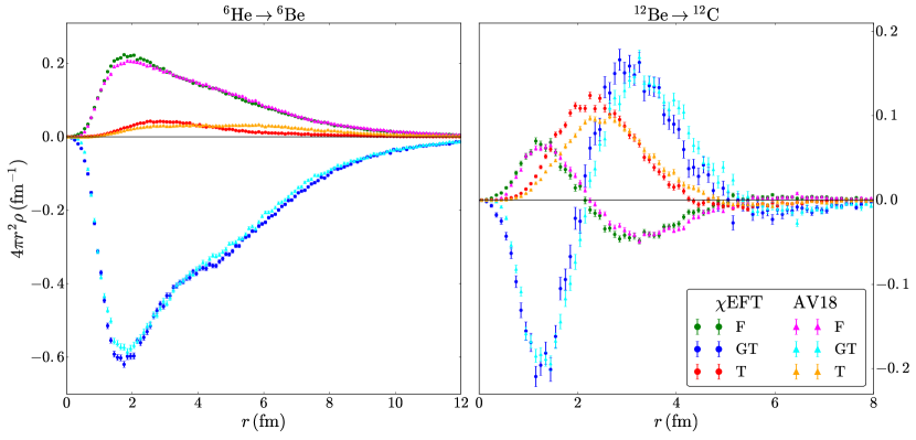
Figure 16: VMC calculations of the Fermi (F), Gamow-Teller (GT), and tensor (T) densities $\rho(r)$ for ⁶He$\rightarrow^{6}$Be (left panel) and ¹²Be$\rightarrow^{12}$C (right panel) decays with two potentials, labeled AV18 and $\chi$EFT.

In order to compare the long- and short-range contributions we define, similarly to Eq. (153), the transition densities

$$C_{\rm L,S}(r)=4\pi R_{A}\,\langle\Psi_{f}|\sum_{a,b}V_{\nu\,\rm L,S}(r_{ab})\,\delta(r_{ab}-r)|\Psi_{i}\rangle\,,\quad M_{\rm L,S}=\int dr\,C_{\rm L,S}(r)$$ (165)

where the conventional factor $\propto R_{A}=1.2\,A^{1/3}$ fm was introduced to make the $A$-nucleon matrix element dimensionless. These densities are plotted in Fig. 17. Integrating $C_{\rm L,S}(r)$ over $r$ yields the values for the matrix elements $M_{i}$ shown in Table 3, where we split the long-range neutrino potential in its Fermi, Gamow-Teller, and tensor components

$$M_{i}=4\pi R_{A}\int dr\,V_{i}(r)(4\pi r^{2}\rho_{i}(r)),\quad i\in\{F,\,GT,\,T\}.$$ (166)

The neutrino potentials $V_{F,\,GT,T}(r)$ are defined in Eq. (30), and $M_{L}=M_{F}-g_{A}^{2}(M_{GT}+M_{T})$.

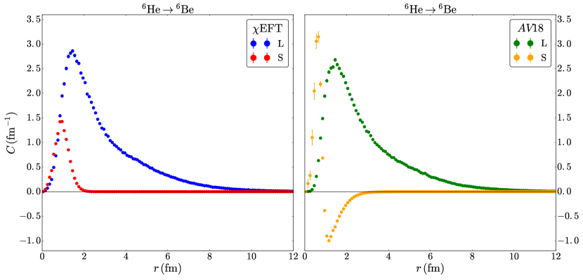
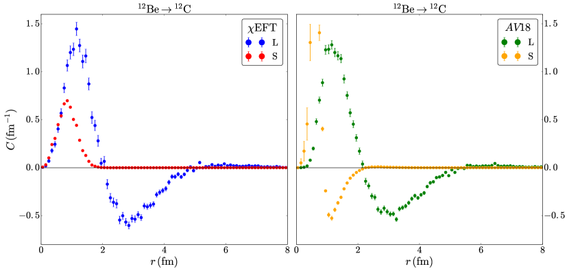
Figure 17: VMC calculations of the long- (L) and short- (S) range transition densities $C(r)$ for ⁶He$\rightarrow^{6}$Be (upper panel) and ¹²Be$\rightarrow^{12}$C (bottom panel) decays with two potentials, labeled $\chi$EFT (left) and AV18 (right).

$A$	Model	$M_{F}$	$M_{GT}$	$M_{T}$	$M_{\rm L}$	$M_{\rm S}$
$6$	AV18	1.56	$-3.66$	0.03	7.45	0.48
	$\chi$EFT	1.62	$-3.85$	0.03	7.82	1.15
$12$	AV18	0.198	$-0.349$	0.068	0.653	0.518
	$\chi$EFT	0.223	$-0.394$	0.083	0.725	0.533

Table 3: VMC results for the dimensionless matrix elements of the long- (L) and short- (S) range neutrino-exchange potentials, defined in Eqs. (165) and (166). For each row, the total long-distance entry $M_{\rm L}$ is obtained via the combination $M_{F}-g_{A}^{2}(M_{GT}+M_{T})$ of its Fermi (F), Gamow-Teller (GT), and tensor (T) components.

The matrix elements of the long-range neutrino potentials obtained with the AV18 and $\chi$EFT models are in good agreement with each other, and with the results of Ref. Pastore et al. (2018b), which used the same AV18 model described above for the nuclear Hamiltonian and “clusterized” wavefunctions obtained by allowing for the formation of clusters in the $p$ shell Nollett et al. (2001). In contrast, the profile of the matrix element of the short-range neutrino potential is sensitive to the model, which for the $\Delta I=0$ transition translates into an uncertainty of a factor 2 in the integrated density. For $\Delta I=2$, the integrated density is much less sensitive to the model.

With the assumption $g_{\nu}^{\rm NN}={\cal C}_{1}={\cal C}_{2}$, the short-range component of the neutrino potential amounts to only $5-15$% of the long-range component in the total ⁶He$\rightarrow{}^{6}$Be amplitude. As for the $nn\rightarrow pp$ transition discussed in Sec. VII.3, the smallness is mostly due to the monotonic long tail of the distribution seen in the top panel of Fig. 17, which is a feature of $\Delta I=0$ transitions.

In contrast, for the $\Delta I=2$ transition the orthogonality of the wavefunctions implies a cancellation between the long-range contributions from $r\lesssim 2$ fm and $r\gtrsim 2$ fm, seen in the lower panel of Fig. 17. In this case, the contribution of $g_{\nu}^{\rm NN}={\cal C}_{1}={\cal C}_{2}$ is a sizable $75-80$% of the total long-range contribution. Although Fig. 17 appears to show a higher degree of cancellation compared to many-body calculations in experimentally relevant nuclei, the node in the density is a robust feature of $\Delta I=2$ transitions Šimkovic et al. (2008); Menéndez et al. (2009). We thus expect the contribution of the short-range operator $g_{\nu}^{\rm NN}$ to be non-negligible.

We caution that these results are based on the arbitrary choice ${\cal C}_{1}={\cal C}_{2}$ dictated by the current undetermined value of ${\cal C}_{2}$. Using the more general assumption $\mathcal{C}_{2}=\alpha\,\mathcal{C}_{1}$ as in Eq. (154) leads to a simple rescaling of the last column of Table 3 by $\kappa=2/(1+\alpha)$. For the ¹²Be $\rightarrow$ ¹²C transition, the short-range component of $V_{\nu}$ can be reduced to a $20$% ($-20$%) correction only for large values for $\alpha\approx 6$ ($\alpha\approx-8$), which would require a sizable deviation from the power-counting expectation $\mathcal{C}_{1}\sim\mathcal{C}_{2}$.

Standard derivations of the $0\nu\beta\beta$ transition operator include short-range effects by introducing the axial, vector, and weak magnetic form factors of the nucleon. We stress that in the analysis of CIB in $N\!N$ scattering the vector form factor is included in both AV18 and $\chi$EFT photon-exchange potentials. However, it does not capture the entire short-range dynamics, which results in non-zero $C_{0}^{\rm IT}$ and $v^{cd}_{S1}(r)$. The contribution of weak magnetism induces corrections to the GT and T potentials Šimkovic et al. (1999), which neglecting the momentum dependence of the magnetic form factor are Pastore et al. (2018b)

$$V_{GT,M\!M}(r)=\frac{(1+\kappa_{1})^{2}}{6g_{A}^{2}m_{N}^{2}}\,\delta^{(3)}({\mathbf{r}})\,,\qquad V_{T,M\!M}(r)=\frac{(1+\kappa_{1})^{2}}{16\pi g_{A}^{2}m_{N}^{2}}\,\frac{1}{r^{3}}\,.\\$$ (167)

$V_{GT,M\!M}$ provides a shift in $g_{\nu}^{\rm NN}$, with coefficient determined by the isovector magnetic moment. The matrix element of $V_{GT,M\!M}$ is however much smaller than the short-range component shown in Table 3. Using the $\chi$EFT wavefunctions we find for example

$$M_{GT,M\!M}(^{6}{\rm He}\rightarrow\,^{6}\mathrm{Be})=-0.10\,,\qquad M_{GT,M\!M}(^{12}{\rm Be}\rightarrow\,^{12}{\rm C})=-0.060\,,$$ (168)

where $M_{GT,MM}$ is defined as in Eq. (166), with $V_{GT}\rightarrow V_{GT,MM}$. Eq. (168) is to be compared to the contributions of $g_{\nu}^{\rm NN}$ in Table 3. This result is a reflection of the fact that CIB data in $N\!N$ scattering indicate the need for an independent local operator, whose coefficient is large and not determined by couplings in the single-nucleon sector. While the extrapolation from CIB to $0\nu\beta\beta$ relies on the uncontrolled assumption ${\cal C}_{1}={\cal C}_{2}$, the results provide strong evidence for the importance of short-range dynamics in $0\nu\beta\beta$.

IX Conclusion

Neutrinoless double-beta decay is the most sensitive laboratory probe of the Majorana nature of neutrinos. The limits on the electron-neutrino Majorana mass from current data, or its extraction from future observations, rely on calculations of $0\nu\beta\beta$ nuclear matrix elements. The calculation of these transition matrix elements in nuclei such as ⁷⁶Ge or ¹³⁶Xe starting from QCD is a daunting task. Nuclear EFTs can help bridge this gap by deriving interactions and transition operators that capture the symmetries of QCD and providing a theoretically consistent framework that can be improved order by order. Nuclear matrix elements of light nuclei, while not directly experimentally accessible, play an important role in establishing such a framework. The first ab initio calculations of $0\nu\beta\beta$ matrix elements, in which nuclear wavefunctions are computed using chiral interactions that are fitted to the properties of two- and three-nucleon systems, are starting to appear as part of a concerted effort toward the reduction of theoretical uncertainties in $0\nu\beta\beta$. In this paper, we derived the $0\nu\beta\beta$ transition operator consistent with these interactions for the case of LNV mediated by light Majorana neutrinos.

Our main findings can be summarized as follows:

• The $0\nu\beta\beta$ transition operator mediated by light Majorana neutrinos has both a long-range and a short-range component at leading order in $\chi$EFT. The long-range component can be expressed in terms of the couplings of nucleons and pions to the axial and vector weak currents, while the short-range component is parametrized by a contact operator whose coefficient, $g_{\nu}^{\rm NN}$, encodes nontrivial QCD dynamics and is at the moment unknown. The need for a short-range component of the $0\nu\beta\beta$ transition operator emerges clearly by studying the $nn\rightarrow pp\,e^{-}e^{-}$ scattering amplitude in various regularization schemes, as done in Sec. IV. The matrix element of the long-range neutrino potential, $V_{\nu}$, between two incoming neutrons and two outgoing protons in the ${}^{1}S_{0}$ channel depends logarithmically on the short-range regulator. Observables can only be made regulator-independent by inclusion of a leading-order short-range LNV operator. Similar sensitivity to UV physics appears in other processes involving potentials with Coulombic behavior that act in the ${}^{1}S_{0}$ channel, for instance charge-independence breaking. The analysis of Sec. VII shows that to reproduce the observed combination of scattering lengths $a_{nn}+a_{pp}-2a_{np}$ in the ${}^{1}S_{0}$ channel, charge-independence-breaking counterterms need to appear at $\mathcal{O}(e^{2})$. They are thus enhanced by $(4\pi)^{2}$, or two powers in the $\chi$EFT power counting, with respect to Weinberg’s power counting. The enhanced contribution of short-range dynamics to charge-independence breaking is observed in both chiral and phenomenological $N\!N$ potentials Epelbaum et al. (2015); Piarulli et al. (2016); Wiringa et al. (1995); Machleidt (2001).

• There is no need for the enhancement of short-range LNV operators in higher partial waves, such as the ${}^{3}P_{J}$ or ${}^{1}D_{2}$. This can be expected in channels where the pion-exchange tensor force is absent or repulsive, like the ${}^{1}D_{2}$ and ${}^{3}P_{1}$ channels. While the attractive nature of the tensor force requires the promotion of an $N\!N$ contact operator to leading order Nogga et al. (2005), once strong interactions are properly renormalized, the matrix element of the long-range neutrino potential is cutoff independent and does not require additional renormalization. We thus expect short-range LNV operators in $P$ and $D$ waves to follow Weinberg’s counting.

• There is no evidence for a short-range momentum-dependent counterterm at next-to-leading order in $\chi$EFT. The NLO analysis of the scattering amplitude was discussed in Sec. VI, in a variety of schemes. In dimensional regularization, the scale invariance of the amplitude requires inclusion of the derivative operator $g_{2\nu}^{\rm NN}$ at NLO, but its coefficient is not independent, and is determined in terms of known couplings. The NLO corrections to $\mathcal{A}_{\nu}$ then purely stem from NLO corrections to the ${}^{1}S_{0}$ strong scattering amplitude. In a cutoff scheme, we similarly showed that $\mathcal{A}_{\nu}$ at NLO becomes cutoff independent as the cutoff is removed without the inclusion of a momentum-dependent counterterm. The residual cutoff dependence of the NLO $nn\rightarrow pp\,e^{-}e^{-}$ scattering amplitude exhibits a $\ln(\Lambda)/\Lambda$ behavior, which might lead to sizable corrections at moderate values of the cutoff, unless $g_{2\nu}^{\rm NN}$ is introduced with fixed coefficients as in dimensional regularization. Our analysis indicates that an independent $g_{2\nu}^{\rm NN}$ enters the neutrino potential at N²LO, or $\mathcal{O}(Q^{2}/\Lambda_{\chi}^{2})$, the same order as contributions from nucleon form factors, closure corrections, and pion-neutrino loops Cirigliano et al. (2018b). We must say, however, that we cannot completely exclude an independent finite LEC at NLO. While NDA predicts such a term at N²LO, it should be kept in mind that NDA only provides a guide to what should be included in a calculation. A possible way to verify the presence (or lack thereof) of an independent NLO LEC would by connecting $g_{2\nu}^{\rm NN}$ to a CIB-breaking combinations of nucleon-nucleon effective ranges, similar to the connection between $g_{\nu}^{\rm NN}$ and CIB scattering lengths (see next bullet).

• The determination of the LEC $g_{\nu}^{\rm NN}$ requires an LQCD calculation of the $nn\rightarrow pp\,e^{-}e^{-}$ scattering amplitude and its matching to ${/\pi}$EFT or $\chi$EFT. In the absence of an LQCD calculation, we can get an order of magnitude estimate of $g_{\nu}^{\rm NN}$ using symmetry arguments. Isospin symmetry relates $g_{\nu}^{\rm NN}$ to the component of the short-range charge-independence-breaking operators that transform as the product of two left- or two right-handed currents, denoted by ${\cal C}_{1}$ in Sec. VII. However, the short-range charge-independence-breaking operators also have a left-right component, ${\cal C}_{2}$, and $N\!N$ scattering data cannot completely determine $g_{\nu}^{\rm NN}$. Using the naturalness assumption ${\cal C}_{1}\sim{\cal C}_{2}$, we showed the potential impact of the short-range neutrino potential on $0\nu\beta\beta$ matrix elements in light nuclei. In Sec. VIII we computed the matrix elements for the ⁶He $\rightarrow$ ⁶Be ($\Delta I=0$) and ¹²Be $\rightarrow$ ¹²C ($\Delta I=2$) transitions using wavefunctions obtained with the $\chi$EFT interactions of Ref. Piarulli et al. (2016), and a consistent extraction of ${\cal C}_{1}+{\cal C}_{2}$. While its impact on $\Delta I=0$ transitions is moderate, $g_{\nu}^{\rm NN}$ can significantly affect $\Delta I=2$ transitions. This observation reinforces the need for a first-principle calculation of $g_{\nu}^{\rm NN}$, in particular because relative factors in the relation between ${\cal C}_{1}$ and ${\cal C}_{2}$ have $\mathcal{O}(1)$ impact on the final results.

• We cannot at this point address the relatively large uncertainty Engel and Menéndez (2017) in the calculation of the matrix elements of heavier nuclei, which are of experimental interest. Once this issue is resolved, the extraction of the effective neutrino mass $m_{\beta\beta}$ could be significantly affected by the short-range LEC $g_{\nu}^{\rm NN}$. If the effect is similar to that calculated in ¹²Be $\rightarrow$ ¹²C with the assumption ${\cal C}_{1}\sim{\cal C}_{2}$, the nuclear neutrinoless double beta decay amplitude would double. With another natural assumption, it might instead be halved. Or it could also be that the small range suppresses its effects for larger $A$. It would be of great interest to calculate the effects of the leading short-range current in heavier nuclei. We suggest to use, as a starting point, the relation $g_{\nu}^{\rm NN}\rightarrow\frac{{\cal C}_{1}+{\cal C}_{2}}{2}$ and the values of ${\cal C}_{1}+{\cal C}_{2}$ as given in Table 2 corresponding to the strong potential applied to obtain the nuclear wave functions.

The EFT framework presented here can be extended in several directions. One of them involves the inclusion of next-to-next-to-leading-order corrections to the nuclear potential. Such terms play an important role in high-quality descriptions of the $N\!N$ database. At this order, the LNV potentials obtain additional corrections Cirigliano et al. (2018b) that should be consistently included. Three-body LNV operators have been identified as a potential source of “$g_{A}$ quenching” Menéndez et al. (2011); Wang et al. (2018). It would be interesting to extend our $\chi$EFT framework to three-nucleon processes. Our work here has been limited to LNV arising from a light-Majorana-neutrino mass term, but in well-motivated scenarios of beyond-the-Standard Model physics, $0\nu\beta\beta$ decay rates can be dominated by higher-dimensional LNV operators Prezeau et al. (2003); Cirigliano et al. (2017, 2018a); Graf et al. (2018). It was argued in Ref. Cirigliano et al. (2018a) that short-range operators must be promoted to leading order for several higher-dimension LNV operators, but the impact of higher-order corrections has not been investigated so far. Most importantly, calculations of the leading short-range contributions must be carried out for heavier nuclei.

Appendix A LNV and $\Delta I=2$ operators with multiple mass insertions

In this appendix we consider the most important LNV operators with insertions of the quark mass mentioned in Sec. VII: one (App. A.1) and two (App. A.2) mass insertions. A summary is given in App. A.3.

A.1 One mass insertion

The LNV operators involving one quark-mass insertion can be built with the elements $Q_{L,R}$ and $M={\rm diag}\,(m_{u},\,m_{d})$, as well as $u$, $u^{\dagger}$, $N$, and $\bar{N}$. We can choose to work with the slightly different spurions $\mathcal{Q}_{L,R}$ and $M_{\pm}=u^{\dagger}Mu^{\dagger}\pm uM^{\dagger}u$, after which all the building blocks transform only under the diagonal subgroup (i.e. $N\to KN$, $\mathcal{Q}_{L,R}\to K\mathcal{Q}_{L,R}K^{\dagger}$, and $M_{\pm}\to KM_{\pm}K^{\dagger}$) apart from $u$ and $u^{\dagger}$. Thus, whenever an operator includes $u$ and/or $u^{\dagger}$, their indices have to be contracted with each other, giving rise to factors of $u^{\dagger}u=uu^{\dagger}=1$. As a result we can forget about the $u$ matrices and use only the spurions and nucleon fields.

We are interested in the operators that give rise to $\Delta I=2$ transitions in $N\!N$ scattering which can be built from $\mathcal{Q}_{X}\times\mathcal{Q}_{Y}\times M_{\pm}$ (where $X,Y\in L,R$). We will therefore need all the $\bar{5}$ representations that reside in the generic tensor, $T^{abc}_{ijk}=(\mathcal{Q}_{X})^{a}_{i}(\mathcal{Q}_{Y})^{b}_{j}(M_{\pm})^{c}_{k}$, which transforms as $T^{abc}_{ijk}\to K_{aa^{\prime}}K_{bb^{\prime}}K_{cc^{\prime}}T^{a^{\prime}b^{\prime}c^{\prime}}_{i^{\prime}j^{\prime}k^{\prime}}(K^{\dagger})_{i^{\prime}i}(K^{\dagger})_{j^{\prime}j}(K^{\dagger})_{k^{\prime}k}$. This tensor can be rewritten as $\bar{T}^{abc\,ijk}=\epsilon^{ii^{\prime}}\epsilon^{jj^{\prime}}\epsilon^{kk^{\prime}}T^{abc}_{i^{\prime}j^{\prime}k^{\prime}}$, so that all indices transform in the same way, $\bar{T}^{abc\,ijk}\to K_{aa^{\prime}}K_{bb^{\prime}}K_{cc^{\prime}}\bar{T}^{a^{\prime}b^{\prime}c^{\prime}\,i^{\prime}j^{\prime}k^{\prime}}K_{ii^{\prime}}K_{jj^{\prime}}K_{kk^{\prime}}$. One can then show that the largest dimensional representation, the $\bar{7}$, is given by $\bar{T}$ with completely symmetrized indices, the next-largest irrep is the one with two antisymmetrized indices (keeping the rest fully symmetric), while the second largest has two pairs of antisymmetrized indices, etc. Thus, to find all the $\bar{5}$ irreps we need to find all the ways in which to contract $\bar{T}$ with a single $\epsilon^{IJ}$ tensor. There are 5 independent ways of doing this, in agreement with the decomposition of $\bar{2}\otimes\bar{2}\otimes\bar{2}\otimes\bar{2}\otimes\bar{2}\otimes\bar{2}$.

One can then choose to contract the indices of $\bar{T}^{abc\,ijk}$ with the following tensors—after using $T^{abc\,ijk}\epsilon_{ab}=T^{acb\,ijk}\epsilon_{ab}+T^{cba\,ijk}\epsilon_{ab}$, which follows from $p^{I}\epsilon^{JK}+p^{J}\epsilon^{KI}+p^{K}\epsilon^{IJ}=0$, to move indices around:

$$\epsilon^{ck},\quad\epsilon^{jc},\quad\epsilon^{ic},\quad\epsilon^{ak},\quad\epsilon^{bk},$$ (169)

where we pick combinations that lead to multiplication of the matrices in $T$ (without leaving any explicit $\epsilon^{ij}$s). In terms of $T$, this leads to the combinations

$$(\mathcal{Q}_{X})^{a}_{i}(\mathcal{Q}_{Y})^{b}_{j}\,{\rm Tr}\,M_{\pm}\,,\quad(\mathcal{Q}_{X})^{a}_{i}(M_{\pm}\mathcal{Q}_{Y})^{b}_{j}\,,\quad(\mathcal{Q}_{X})^{a}_{i}(\mathcal{Q}_{Y}M_{\pm})^{b}_{j}\,,$$

$$(\mathcal{Q}_{Y})^{a}_{i}(M_{\pm}\mathcal{Q}_{X})^{b}_{j}\,,\quad(\mathcal{Q}_{Y})^{a}_{i}(\mathcal{Q}_{X}M_{\pm})^{b}_{j}\,.$$ (170)

One then still needs to project the remaining indices onto the $\bar{5}$ representation, by demanding the upper/lower indices to be symmetric and traceless (or simply fully symmetric in the case of $\bar{T}$). An explicit form of this projection is

$$A^{a}_{i}B_{j}^{b}\bigg{|}_{\bar{5}} = \frac{1}{2}A^{a}_{i}B^{b}_{j}+\frac{1}{24}({\rm Tr}\,A\,{\rm Tr}\,B-2{\rm Tr}\,AB)(\tau^{I})^{a}_{i}(\tau^{I})^{b}_{j}$$ (171)

$$-\frac{1}{4}\,{\rm Tr}\,A(B_{i}^{a}\delta^{b}_{j}+B_{j}^{b}\delta^{a}_{i})+\frac{1}{8}{\rm Tr}\,A\,{\rm Tr}\,B\delta^{a}_{i}\delta^{b}_{j}+(A\leftrightarrow B)\,.$$

After projecting, one then has to make sure that the combinations of $\mathcal{Q}_{L,R}$ and $M_{+,-}$ have the correct properties under charge conjugation ($C$), parity ($P$), and time reversal ($T$).

All in all, this leads to the following operators,

$$O_{M1}^{(1)} = O_{1}\,{\rm Tr}\,M_{+}\,,\qquad O_{M1}^{(2)}=O_{2}\,{\rm Tr}\,M_{+}\,,\qquad O^{(1)}_{M2}=\bar{N}\mathcal{Q}_{L}N\,\bar{N}\left[\mathcal{Q}_{L},\,M_{-}\right]N-(L\leftrightarrow R)\,,$$

$$O^{(2)}_{M2} = \bar{N}\mathcal{Q}_{L}N\,\bar{N}\left[\mathcal{Q}_{R},\,M_{-}\right]N-\frac{1}{6}\,{\rm Tr}\left(\mathcal{Q}_{L}\left[\mathcal{Q}_{R},\,M_{-}\right]\right)\bar{N}\tau^{I}N\,\bar{N}\tau^{I}N-(L\leftrightarrow R)\,,$$ (172)

where $O_{1,2}$ are the operators without any $M$ insertions,

$$O_{1} = \bar{N}\mathcal{Q}_{L}N\,\bar{N}\mathcal{Q}_{L}N-\frac{1}{6}\,{\rm Tr}\left(\mathcal{Q}_{L}\mathcal{Q}_{L}\right)\bar{N}\tau^{I}N\,\bar{N}\tau^{I}N+(L\leftrightarrow R)\,,$$

$$O_{2} = \bar{N}\mathcal{Q}_{L}N\,\bar{N}\mathcal{Q}_{R}N-\frac{1}{6}\,{\rm Tr}\left(\mathcal{Q}_{L}\mathcal{Q}_{R}\right)\bar{N}\tau^{I}N\,\bar{N}\tau^{I}N+(L\leftrightarrow R)\,.$$ (173)

There are no operators similar to $O^{(1,2)}_{M1}$ with $M_{-}$ instead of $M_{+}$ since Tr$M_{-}=0$. In addition, operators of the form of $O^{(1,2)}_{M2}$ involving $M_{+}$ instead of $M_{-}$ necessarily contain an anticommutator $\{M_{+},\,\mathcal{Q}_{X}\}$, which can be rewritten in terms of $O^{(1,2)}_{M1}$ thanks to the fact that the $\mathcal{Q}_{X}$ are traceless.

For the $N\!N$ vertices without any pions, only the $O_{M1}^{(1,2)}$ operators contribute, simply giving the original operators multiplied by Tr $M$. Instead, the $O^{(1,2)}_{M2}$ operators only induce vertices with two additional pions.

A.2 Two mass insertions

We can use a similar process to find the $\bar{5}$ representations in $T^{abcd}_{ijkl}=(\mathcal{Q}_{X})^{a}_{i}(\mathcal{Q}_{Y})^{b}_{j}(M_{\pm})^{c}_{k}(M_{\pm})^{d}_{l}$. One now has to contract with two epsilon tensors, which can be done in 20 independent ways. However, after choosing a set of ways to contract the indices, not all possibilities contribute, for example due to $P$, $T$, or $C$ properties, or because some of our building blocks are traceless. The operators involving two insertions of the same $M_{\pm}$ take the schematic form

$$O^{(1,2)}_{M_{\pm}^{2}1}={\rm Tr}\,M_{\pm}^{2}O_{1,2}\,\qquad O^{(1,2)}_{M_{+}^{2}2}={\rm Tr}\,\left(M_{+}\right)^{2}O_{1,2},\,$$

$$O^{(1)}_{M_{\pm}^{2}3}: \quad A=\mathcal{Q}_{L}M_{\pm}\mathcal{Q}_{L}\,,\quad B=M_{\pm}\qquad+(L\leftrightarrow R)\,,$$

$$O^{(2)}_{M_{\pm}^{2}3}: \quad A=\mathcal{Q}_{L}M_{\pm}\mathcal{Q}_{R}\,,\quad B=M_{\pm}\qquad+(L\leftrightarrow R)\,,$$

$$O^{(1)}_{M_{\pm}^{2}4}: \quad A=\mathcal{Q}_{L}\,{\rm Tr}\left(M_{\pm}\mathcal{Q}_{L}\right)\,,\quad B=M_{\pm}\qquad+(L\leftrightarrow R)\,,$$

$$O^{(2)}_{M_{\pm}^{2}4}: \quad A=\mathcal{Q}_{L}\,{\rm Tr}\left(M_{\pm}\mathcal{Q}_{R}\right)\,,\quad B=M_{\pm}\qquad+(L\leftrightarrow R)\,,$$

$$O^{(1)}_{M_{\pm}^{2}5}: \quad A=M_{\pm}\mathcal{Q}_{L}\,,\quad B=M_{\pm}\mathcal{Q}_{L}\qquad+(L\leftrightarrow R)+(M_{\pm}\leftrightarrow\mathcal{Q}_{L,R})\,,$$

$$O^{(2)}_{M_{\pm}^{2}5}: \quad A=M_{\pm}\mathcal{Q}_{L}\,,\quad B=M_{\pm}\mathcal{Q}_{R}\qquad+(L\leftrightarrow R)+(M_{\pm}\leftrightarrow\mathcal{Q}_{L,R})\,,$$ (174)

One should use the above expressions for $A$ and $B$ to construct the corresponding operators by projecting them onto the $\bar{5}$ representation using Eq. (171), and subsequently contracting with $\bar{N}^{a}\bar{N}^{b}N^{i}N^{j}$. After doing so the $O^{(1,2)}_{M_{+}^{2}3,4}$ operators do not contribute to $(\bar{N}N)^{2}$ and $(\pi\bar{N}N)^{2}$ vertices, while $O^{(1,2)}_{M_{+}^{2}5}=O^{(1,2)}_{M_{+}^{2}2}/2$ (at least up to two-pion vertices, for $m_{u}=m_{d}$). Instead, the $O^{(1,2)}_{M_{-}^{2}3,4,5}$ operators only give rise to $(\pi\bar{N}N)^{2}$ vertices.

The remaining operators are proportional to $M_{-}M_{+}$, and take the form

$$O_{M_{+}M_{-}1}^{(1)}: \quad A=\mathcal{Q}_{L}M_{+},\quad B=\mathcal{Q}_{L}M_{-}\qquad-(L\leftrightarrow R)-(M_{\pm}\leftrightarrow\mathcal{Q}_{L,R})\,,$$

$$O_{M_{+}M_{-}1}^{(2)}: \quad A=\mathcal{Q}_{R}M_{+},\quad B=\mathcal{Q}_{L}M_{-}\qquad-(L\leftrightarrow R)-(M_{\pm}\leftrightarrow\mathcal{Q}_{L,R})\,,$$

$$O_{M_{+}M_{-}2}^{(1)}: \quad A=\left[M_{-},\,\mathcal{Q}_{L}\right]\,,\quad B=\mathcal{Q}_{L}\,{\rm Tr}\,M_{+}\qquad-(L\leftrightarrow R)\,,$$

$$O_{M_{+}M_{-}2}^{(2)}: \quad A=\left[M_{-},\,\mathcal{Q}_{R}\right]\,,\quad B=\mathcal{Q}_{L}\,{\rm Tr}\,M_{+}\qquad-(L\leftrightarrow R)\,$$

$$O_{M_{+}M_{-}3}^{(2)}: \quad A=M_{-}\,,\quad B=\mathcal{Q}_{R}M_{+}\mathcal{Q}_{L}\qquad-(L\leftrightarrow R)\,.$$ (175)

After projecting, these operators turn out to be similar to the ones with one $M$ insertion, we have $2O_{M_{+}M_{-}1}^{(1,2)}=-O_{M_{+}M_{-}2}^{(1,2)}=O_{M2}^{(1,2)}\,{\rm Tr}\,M_{+}$ and $2O_{M_{+}M_{-}3}^{(2)}=O_{M2}^{(2)}\,{\rm Tr}\,M_{+}$, up to two-pion vertices (for $m_{u}=m_{d}$).

To get the operators in Eqs. (174) and (175) we again used identities like the one above Eq. (169) to pick combinations that lead to multiplication of the matrices in $T$ (to avoid explicit $\epsilon^{ij}$s). In addition, we used the fact that $\mathcal{Q}_{X}$ and $M_{-}$ are traceless. Apart from those assumptions, Eqs. (174) and (175) provide a complete basis of operators.

A.3 Mass-insertion summary

With the above results in hand, the effective ${\cal C}_{1,2}$ couplings defined in Sec. VII become

$${\cal C}_{1,2}^{eff}={\cal C}_{1,2}+4\bar{m}C_{M1}^{(1,2)}+4\bar{m}^{2}\left(2C_{M_{+}^{2}1}^{(1,2)}+4C_{M_{+}^{2}2}^{(1,2)}+2C_{M_{+}^{2}5}^{(1,2)}\right)\,,$$ (176)

where we set $m_{u,d}=\bar{m}$. Here the second term should absorb the divergence proportional to $D_{2}$, while the third term (in brackets) should do so for the $D_{2}^{2}$ term.

The procedure can be extended to a larger number of mass insertions straightforwardly but painfully.

Appendix B The $\overline{\rm MS}$ scheme

Although one can in principle calculate the $N\!N$ amplitudes analytically in $\overline{\rm MS}$ within ${/\pi}$EFT, this is no longer the case in $\chi$EFT. Here one needs to numerically evaluate quantities such as $\chi_{{\mathbf{p}}}^{\pm}(r)$, $G_{E}^{\pm}({\mathbf{r}},0)$, and $K_{E}$ which all involve an arbitrary number of pion exchanges. To do so we closely follow the method described in Ref. Kaplan et al. (1996), to which we refer for further details.

The strategy is to first use an intermediate scheme in which one solves the Schrödinger equation by imposing the boundary conditions at $r=1/\lambda$, where $\lambda$ is a regulator. This results in a regular and an irregular solution, the latter of which will depend on the regulator, $\lambda$. The regular solution obtained in this way allows one to determine $\chi_{{\mathbf{p}}}^{\pm}(r)$, while a combination of the regular and irregular solutions give rise to $G_{E}^{\pm}({\mathbf{r}},0)$ and $K_{E}$. Because the latter of these quantities is regulator- and scheme-independent it can be used to translate from the $\lambda$ scheme to the $\overline{\rm MS}$ scheme. In particular, we have

$$\frac{1}{\tilde{C}(\lambda)}-G_{E}^{\pm}(0,0)\big{|}_{\lambda}=\frac{1}{\tilde{C}(\mu)_{\overline{\rm MS}}}-G_{E}^{\pm}(0,0)\big{|}_{\overline{\rm MS}}\,.$$ (177)

In addition, one knows that differences between the $G_{E}^{\pm}(0,0)$ in the two schemes can only arise from their divergent parts, and only the first two diagrams in $G_{E}^{\pm}(0,0)$ (i.e. the parts that have zero and one insertion of $V_{\pi}$ after expanding Eq. (38)) lead to divergences. This allows one to relate both $\tilde{C}$ and $G_{E}^{\pm}(0,0)$ in $\overline{\rm MS}$ to terms that can be analytically computed and quantities that can be numerically obtained in the $\lambda$ scheme.

For example, applying this procedure to $N\!N$ scattering in the ${}^{1}S_{0}$ channel leads to

$$\frac{1}{\tilde{C}(\mu)}+\frac{\alpha_{\pi}m_{N}^{2}}{8\pi}\,\ln\frac{\mu^{2}}{m_{\pi}^{2}}\simeq-0.24\,{\rm fm}^{-2},$$ (178)

which is in agreement with the results of Ref. Kaplan et al. (1996). The same procedure can be used to evaluate the $\Delta L=2$ amplitudes in Eqs. (61) and (86), as well as the $nn$, $pp$, and $np$ amplitudes in the presence of isospin violation as discussed in Sec. VII.2.

References

- Aseev et al. (2011) V. N. Aseev et al. (Troitsk), “An upper limit on electron antineutrino mass from Troitsk experiment,” Phys. Rev. D84, 112003 (2011), arXiv:1108.5034 [hep-ex] .
- Akrami et al. (2018) Y. Akrami et al. (Planck), “Planck 2018 results. I. Overview and the cosmological legacy of Planck,” (2018), arXiv:1807.06205 [astro-ph.CO] .
- Minkowski (1977) Peter Minkowski, “ at a Rate of One Out of Muon Decays?” Phys. Lett. 67B, 421–428 (1977).
- Mohapatra and Senjanovic (1980) Rabindra N. Mohapatra and Goran Senjanovic, “Neutrino Mass and Spontaneous Parity Violation,” Phys. Rev. Lett. 44, 912 (1980).
- Gell-Mann et al. (1979) Murray Gell-Mann, Pierre Ramond, and Richard Slansky, “Complex Spinors and Unified Theories,” Supergravity Workshop Stony Brook, New York, September 27-28, 1979, Conf. Proc. C790927, 315–321 (1979), arXiv:1306.4669 [hep-th] .
- Schechter and Valle (1982) J. Schechter and J. W. F. Valle, “Neutrinoless Double beta Decay in SU(2) x U(1) Theories,” Phys. Rev. D25, 2951 (1982).
- Haxton and Stephenson (1984) W. C. Haxton and G. J. Stephenson, “Double beta Decay,” Prog. Part. Nucl. Phys. 12, 409–479 (1984).
- Gando et al. (2013) A. Gando et al. (KamLAND-Zen), “Limit on Neutrinoless Decay of 136Xe from the First Phase of KamLAND-Zen and Comparison with the Positive Claim in 76Ge,” Phys. Rev. Lett. 110, 062502 (2013), arXiv:1211.3863 [hep-ex] .
- Agostini et al. (2013) M. Agostini et al. (GERDA), “Results on Neutrinoless Double- Decay of 76Ge from Phase I of the GERDA Experiment,” Phys. Rev. Lett. 111, 122503 (2013), arXiv:1307.4720 [nucl-ex] .
- Albert et al. (2014) J. B. Albert et al. (EXO-200), “Search for Majorana neutrinos with the first two years of EXO-200 data,” Nature 510, 229–234 (2014), arXiv:1402.6956 [nucl-ex] .
- Andringa et al. (2016) S. Andringa et al. (SNO+), “Current Status and Future Prospects of the SNO+ Experiment,” Adv. High Energy Phys. 2016, 6194250 (2016), arXiv:1508.05759 [physics.ins-det] .
- Gando et al. (2016) A. Gando et al. (KamLAND-Zen), “Search for Majorana Neutrinos near the Inverted Mass Hierarchy Region with KamLAND-Zen,” Phys. Rev. Lett. 117, 082503 (2016), [Addendum: Phys. Rev. Lett.117,no.10,109903(2016)], arXiv:1605.02889 [hep-ex] .
- Elliott et al. (2016) S. R. Elliott et al., “Initial Results from the MAJORANA DEMONSTRATOR,” (2016) arXiv:1610.01210 [nucl-ex] .
- Agostini et al. (2017) M. Agostini et al., “Background-free search for neutrinoless double- decay of 76Ge with GERDA,” (2017), 10.1038/nature21717, [Nature544,47(2017)], arXiv:1703.00570 [nucl-ex] .
- Aalseth et al. (2018) C. E. Aalseth et al. (Majorana), “Search for Neutrinoless Double-? Decay in 76Ge with the Majorana Demonstrator,” Phys. Rev. Lett. 120, 132502 (2018), arXiv:1710.11608 [nucl-ex] .
- Albert et al. (2018) J. B. Albert et al. (EXO), “Search for Neutrinoless Double-Beta Decay with the Upgraded EXO-200 Detector,” Phys. Rev. Lett. 120, 072701 (2018), arXiv:1707.08707 [hep-ex] .
- Alduino et al. (2018) C. Alduino et al. (CUORE), “First Results from CUORE: A Search for Lepton Number Violation via Decay of 130Te,” Phys. Rev. Lett. 120, 132501 (2018), arXiv:1710.07988 [nucl-ex] .
- Agostini et al. (2018) M. Agostini et al. (GERDA), “Improved Limit on Neutrinoless Double- Decay of 76Ge from GERDA Phase II,” Phys. Rev. Lett. 120, 132503 (2018), arXiv:1803.11100 [nucl-ex] .
- Azzolini et al. (2018) O. Azzolini et al. (CUPID-0), “First Result on the Neutrinoless Double- Decay of with CUPID-0,” Phys. Rev. Lett. 120, 232502 (2018), arXiv:1802.07791 [nucl-ex] .
- Anton et al. (2019) G. Anton et al., “Search for Neutrinoless Double-Beta Decay with the Complete EXO-200 Dataset,” (2019), arXiv:1906.02723 [hep-ex] .
- Prezeau et al. (2003) Gary Prezeau, M. Ramsey-Musolf, and Petr Vogel, “Neutrinoless double beta decay and effective field theory,” Phys. Rev. D68, 034016 (2003), arXiv:hep-ph/0303205 [hep-ph] .
- Graesser (2017) Michael L. Graesser, “An electroweak basis for neutrinoless double decay,” JHEP 08, 099 (2017), arXiv:1606.04549 [hep-ph] .
- Cirigliano et al. (2017) V. Cirigliano, W. Dekens, J. de Vries, M. L. Graesser, and E. Mereghetti, “Neutrinoless double beta decay in chiral effective field theory: lepton number violation at dimension seven,” JHEP 12, 082 (2017), arXiv:1708.09390 [hep-ph] .
- Cirigliano et al. (2018a) V. Cirigliano, W. Dekens, J. de Vries, M. L. Graesser, and E. Mereghetti, “A neutrinoless double beta decay master formula from effective field theory,” JHEP 12, 097 (2018a), arXiv:1806.02780 [hep-ph] .
- Weinberg (1979a) Steven Weinberg, “Baryon and Lepton Nonconserving Processes,” Phys. Rev. Lett. 43, 1566–1570 (1979a).
- Weinberg (1979b) Steven Weinberg, “Phenomenological Lagrangians,” Physica A96, 327 (1979b).
- Weinberg (1990) Steven Weinberg, “Nuclear forces from chiral Lagrangians,” Phys. Lett. B251, 288–292 (1990).
- Weinberg (1991) Steven Weinberg, “Effective chiral Lagrangians for nucleon - pion interactions and nuclear forces,” Nucl. Phys. B363, 3–18 (1991).
- Engel and Menéndez (2017) Jonathan Engel and Javier Menéndez, “Status and Future of Nuclear Matrix Elements for Neutrinoless Double-Beta Decay: A Review,” Rept. Prog. Phys. 80, 046301 (2017), arXiv:1610.06548 [nucl-th] .
- Ejiri et al. (2019) H. Ejiri, J. Suhonen, and K. Zuber, “Neutrino–nuclear responses for astro-neutrinos, single beta decays and double beta decays,” Phys. Rept. 797, 1–102 (2019).
- Cirigliano et al. (2018b) Vincenzo Cirigliano, Wouter Dekens, Emanuele Mereghetti, and André Walker-Loud, “Neutrinoless double- decay in effective field theory: The light-Majorana neutrino-exchange mechanism,” Phys. Rev. C97, 065501 (2018b), arXiv:1710.01729 [hep-ph] .
- Cirigliano et al. (2018c) Vincenzo Cirigliano, Wouter Dekens, Jordy De Vries, Michael L. Graesser, Emanuele Mereghetti, Saori Pastore, and Ubirajara van Kolck, “New Leading Contribution to Neutrinoless Double-Beta Decay,” Phys. Rev. Lett. 120, 202001 (2018c), arXiv:1802.10097 [hep-ph] .
- Machleidt and Entem (2011) R. Machleidt and D. R. Entem, “Chiral effective field theory and nuclear forces,” Phys. Rept. 503, 1–75 (2011), arXiv:1105.2919 [nucl-th] .
- Piarulli et al. (2015) M. Piarulli, L. Girlanda, R. Schiavilla, R. Navarro Pérez, J. E. Amaro, and E. Ruiz Arriola, “Minimally nonlocal nucleon-nucleon potentials with chiral two-pion exchange including resonances,” Phys. Rev. C91, 024003 (2015), arXiv:1412.6446 [nucl-th] .
- Epelbaum et al. (2015) E. Epelbaum, H. Krebs, and U. G. Meißner, “Improved chiral nucleon-nucleon potential up to next-to-next-to-next-to-leading order,” Eur. Phys. J. A51, 53 (2015), arXiv:1412.0142 [nucl-th] .
- Ekström et al. (2015) A. Ekström, G. R. Jansen, K. A. Wendt, G. Hagen, T. Papenbrock, B. D. Carlsson, C. Forssén, M. Hjorth-Jensen, P. Navrátil, and W. Nazarewicz, “Accurate nuclear radii and binding energies from a chiral interaction,” Phys. Rev. C91, 051301 (2015), arXiv:1502.04682 [nucl-th] .
- Piarulli et al. (2016) Maria Piarulli, Luca Girlanda, Rocco Schiavilla, Alejandro Kievsky, Alessandro Lovato, Laura E. Marcucci, Steven C. Pieper, Michele Viviani, and Robert B. Wiringa, “Local chiral potentials with -intermediate states and the structure of light nuclei,” Phys. Rev. C94, 054007 (2016), arXiv:1606.06335 [nucl-th] .
- Reinert et al. (2018) P. Reinert, H. Krebs, and E. Epelbaum, “Semilocal momentum-space regularized chiral two-nucleon potentials up to fifth order,” Eur. Phys. J. A54, 86 (2018), arXiv:1711.08821 [nucl-th] .
- Wiringa et al. (1995) R. B. Wiringa, V. G. J. Stoks, and R. Schiavilla, “An Accurate nucleon-nucleon potential with charge independence breaking,” Phys. Rev. C51, 38–51 (1995), arXiv:nucl-th/9408016 [nucl-th] .
- Machleidt (2001) R. Machleidt, “The High precision, charge dependent Bonn nucleon-nucleon potential (CD-Bonn),” Phys. Rev. C63, 024001 (2001), arXiv:nucl-th/0006014 [nucl-th] .
- Nogga et al. (2005) A. Nogga, R. G. E. Timmermans, and U. van Kolck, “Renormalization of one-pion exchange and power counting,” Phys. Rev. C72, 054006 (2005), arXiv:nucl-th/0506005 [nucl-th] .
- Pavón Valderrama and Ruiz Arriola (2006) M. Pavón Valderrama and E. Ruiz Arriola, “Renormalization of NN interaction with chiral two pion exchange potential: Non-central phases,” Phys. Rev. C74, 064004 (2006), [Erratum: Phys. Rev.C75,059905(2007)], arXiv:nucl-th/0507075 [nucl-th] .
- Long and Yang (2012) Bingwei Long and C.-J. Yang, “Short-range nuclear forces in singlet channels,” Phys. Rev. C86, 024001 (2012), arXiv:1202.4053 [nucl-th] .
- Manohar and Georgi (1984) Aneesh Manohar and Howard Georgi, “Chiral Quarks and the Nonrelativistic Quark Model,” Nucl. Phys. B234, 189–212 (1984).
- Beane et al. (2002) S. R. Beane, Paulo F. Bedaque, M. J. Savage, and U. van Kolck, “Towards a perturbative theory of nuclear forces,” Nucl. Phys. A700, 377–402 (2002), arXiv:nucl-th/0104030 [nucl-th] .
- Pavón Valderrama and Phillips (2015) M. Pavón Valderrama and Daniel R. Phillips, “Power Counting of Contact-Range Currents in Effective Field Theory,” Phys. Rev. Lett. 114, 082502 (2015), arXiv:1407.0437 [nucl-th] .
- Wang et al. (2018) Long-Jun Wang, Jonathan Engel, and Jiang Ming Yao, “Quenching of nuclear matrix elements for decay by chiral two-body currents,” Phys. Rev. C98, 031301 (2018), arXiv:1805.10276 [nucl-th] .
- Miller and Spencer (1976) Gerald A. Miller and James E. Spencer, “A Survey of Pion Charge-Exchange Reactions with Nuclei,” Annals Phys. 100, 562 (1976).
- Simkovic et al. (2009) Fedor Simkovic, Amand Faessler, Herbert Muther, Vadim Rodin, and Markus Stauf, “The 0 nu bb-decay nuclear matrix elements with self-consistent short-range correlations,” Phys. Rev. C79, 055501 (2009), arXiv:0902.0331 [nucl-th] .
- Engel et al. (2011) J. Engel, J. Carlson, and R. B. Wiringa, “Jastrow functions in double-beta decay,” Phys. Rev. C83, 034317 (2011), arXiv:1101.0554 [nucl-th] .
- Benhar et al. (2014) Omar Benhar, Riccardo Biondi, and Enrico Speranza, “Short-range correlation effects on the nuclear matrix element of neutrinoless double-beta decay,” Phys. Rev. C90, 065504 (2014), arXiv:1401.2030 [nucl-th] .
- Pastore et al. (2018a) S. Pastore, A. Baroni, J. Carlson, S. Gandolfi, Steven C. Pieper, R. Schiavilla, and R. B. Wiringa, “Quantum Monte Carlo calculations of weak transitions in nuclei,” Phys. Rev. C97, 022501 (2018a), arXiv:1709.03592 [nucl-th] .
- Gysbers et al. (2019) P. Gysbers et al., “Discrepancy between experimental and theoretical -decay rates resolved from first principles,” Nature Phys. 15, 428–431 (2019), arXiv:1903.00047 [nucl-th] .
- Shanahan et al. (2017) Phiala E. Shanahan, Brian C. Tiburzi, Michael L. Wagman, Frank Winter, Emmanuel Chang, Zohreh Davoudi, William Detmold, Kostas Orginos, and Martin J. Savage, “The isotensor axial polarisability and lattice QCD input for nuclear double- decay phenomenology,” Phys. Rev. Lett. 119, 062003 (2017), arXiv:1701.03456 [hep-lat] .
- Tiburzi et al. (2017) Brian C. Tiburzi, Michael L. Wagman, Frank Winter, Emmanuel Chang, Zohreh Davoudi, William Detmold, Kostas Orginos, Martin J. Savage, and Phiala E. Shanahan, “Double- Decay Matrix Elements from Lattice Quantum Chromodynamics,” Phys. Rev. D96, 054505 (2017), arXiv:1702.02929 [hep-lat] .
- Feng et al. (2019) Xu Feng, Lu-Chang Jin, Xin-Yu Tuo, and Shi-Cheng Xia, “Light-Neutrino Exchange and Long-Distance Contributions to Decays: An Exploratory Study on ,” Phys. Rev. Lett. 122, 022001 (2019), arXiv:1809.10511 [hep-lat] .
- Cirigliano et al. (2019) Vincenzo Cirigliano, Zohreh Davoudi, Tanmoy Bhattacharya, Taku Izubuchi, Phiala E. Shanahan, Sergey Syritsyn, and Michael L. Wagman, “The Role of Lattice QCD in Searches for Violations of Fundamental Symmetries and Signals for New Physics,” (2019), arXiv:1904.09704 [hep-lat] .
- Nicholson et al. (2018) A. Nicholson et al., “Heavy physics contributions to neutrinoless double beta decay from QCD,” Phys. Rev. Lett. 121, 172501 (2018), arXiv:1805.02634 [nucl-th] .
- Monge-Camacho et al. (2019) Henry Monge-Camacho et al., “Short Range Operator Contributions to decay from LQCD,” in 36th International Symposium on Lattice Field Theory (Lattice 2018) East Lansing, MI, United States, July 22-28, 2018 (2019) arXiv:1904.12055 [hep-lat] .
- Bedaque and van Kolck (1998) Paulo F. Bedaque and U. van Kolck, “Nucleon deuteron scattering from an effective field theory,” Phys. Lett. B428, 221–226 (1998), arXiv:nucl-th/9710073 [nucl-th] .
- Bedaque et al. (1998) Paulo F. Bedaque, H. W. Hammer, and U. van Kolck, “Effective theory for neutron deuteron scattering: Energy dependence,” Phys. Rev. C58, R641–R644 (1998), arXiv:nucl-th/9802057 [nucl-th] .
- Chen et al. (1999) Jiunn-Wei Chen, Gautam Rupak, and Martin J. Savage, “Nucleon-nucleon effective field theory without pions,” Nucl. Phys. A653, 386–412 (1999), arXiv:nucl-th/9902056 [nucl-th] .
- Kong and Ravndal (2000) Xinwei Kong and Finn Ravndal, “Coulomb effects in low-energy proton proton scattering,” Nucl. Phys. A665, 137–163 (2000), arXiv:hep-ph/9903523 [hep-ph] .
- Bedaque et al. (2000) Paulo F. Bedaque, H. W. Hammer, and U. van Kolck, “Effective theory of the triton,” Nucl. Phys. A676, 357–370 (2000), arXiv:nucl-th/9906032 [nucl-th] .
- Bedaque and van Kolck (2002) Paulo F. Bedaque and Ubirajara van Kolck, “Effective field theory for few nucleon systems,” Ann. Rev. Nucl. Part. Sci. 52, 339–396 (2002), arXiv:nucl-th/0203055 [nucl-th] .
- Vanasse (2013) Jared Vanasse, “Fully Perturbative Calculation of Scattering to Next-to-next-to-leading-order,” Phys. Rev. C88, 044001 (2013), arXiv:1305.0283 [nucl-th] .
- König et al. (2016) Sebastian König, Harald W. Grießhammer, H.-W. Hammer, and U. van Kolck, “Effective theory of 3H and 3He,” J. Phys. G43, 055106 (2016), arXiv:1508.05085 [nucl-th] .
- Platter et al. (2005) L. Platter, H. W. Hammer, and Ulf-G. Meissner, “On the correlation between the binding energies of the triton and the alpha-particle,” Phys. Lett. B607, 254–258 (2005), arXiv:nucl-th/0409040 [nucl-th] .
- Stetcu et al. (2007) I. Stetcu, B. R. Barrett, and U. van Kolck, “No-core shell model in an effective-field-theory framework,” Phys. Lett. B653, 358–362 (2007), arXiv:nucl-th/0609023 [nucl-th] .
- Contessi et al. (2017) L. Contessi, A. Lovato, F. Pederiva, A. Roggero, J. Kirscher, and U. van Kolck, “Ground-state properties of 4He and 16O extrapolated from lattice QCD with pionless EFT,” Phys. Lett. B772, 839–848 (2017), arXiv:1701.06516 [nucl-th] .
- Bansal et al. (2018) A. Bansal, S. Binder, A. Ekström, G. Hagen, G. R. Jansen, and T. Papenbrock, “Pion-less effective field theory for atomic nuclei and lattice nuclei,” Phys. Rev. C98, 054301 (2018), arXiv:1712.10246 [nucl-th] .
- Barnea et al. (2015) N. Barnea, L. Contessi, D. Gazit, F. Pederiva, and U. van Kolck, “Effective Field Theory for Lattice Nuclei,” Phys. Rev. Lett. 114, 052501 (2015), arXiv:1311.4966 [nucl-th] .
- Beane et al. (2015) Silas R. Beane, Emmanuel Chang, William Detmold, Kostas Orginos, Assumpta Parreño, Martin J. Savage, and Brian C. Tiburzi (NPLQCD), “Ab initio Calculation of the Radiative Capture Process,” Phys. Rev. Lett. 115, 132001 (2015), arXiv:1505.02422 [hep-lat] .
- Kirscher et al. (2015) Johannes Kirscher, Nir Barnea, Doron Gazit, Francesco Pederiva, and Ubirajara van Kolck, “Spectra and Scattering of Light Lattice Nuclei from Effective Field Theory,” Phys. Rev. C92, 054002 (2015), arXiv:1506.09048 [nucl-th] .
- Savage et al. (2017) Martin J. Savage, Phiala E. Shanahan, Brian C. Tiburzi, Michael L. Wagman, Frank Winter, Silas R. Beane, Emmanuel Chang, Zohreh Davoudi, William Detmold, and Kostas Orginos, “Proton-Proton Fusion and Tritium Decay from Lattice Quantum Chromodynamics,” Phys. Rev. Lett. 119, 062002 (2017), arXiv:1610.04545 [hep-lat] .
- Kaplan et al. (1998a) David B. Kaplan, Martin J. Savage, and Mark B. Wise, “A New expansion for nucleon-nucleon interactions,” Phys. Lett. B424, 390–396 (1998a), arXiv:nucl-th/9801034 [nucl-th] .
- Kaplan et al. (1998b) David B. Kaplan, Martin J. Savage, and Mark B. Wise, “Two nucleon systems from effective field theory,” Nucl. Phys. B534, 329–355 (1998b), arXiv:nucl-th/9802075 [nucl-th] .
- Beane et al. (1998) S. R. Beane, T. D. Cohen, and Daniel R. Phillips, “The Potential of effective field theory in N N scattering,” Nucl. Phys. A632, 445–469 (1998), arXiv:nucl-th/9709062 [nucl-th] .
- van Kolck (1999) U. van Kolck, “Effective field theory of short range forces,” Nucl. Phys. A645, 273–302 (1999), arXiv:nucl-th/9808007 [nucl-th] .
- Bedaque et al. (1999a) Paulo F. Bedaque, H. W. Hammer, and U. van Kolck, “Renormalization of the three-body system with short range interactions,” Phys. Rev. Lett. 82, 463–467 (1999a), arXiv:nucl-th/9809025 [nucl-th] .
- Bedaque et al. (1999b) Paulo F. Bedaque, H. W. Hammer, and U. van Kolck, “The Three boson system with short range interactions,” Nucl. Phys. A646, 444–466 (1999b), arXiv:nucl-th/9811046 [nucl-th] .
- Pandharipande et al. (2005) V. R. Pandharipande, Daniel R. Phillips, and U. van Kolck, “Delta effects in pion-nucleon scattering and the strength of the two-pion-exchange three-nucleon interaction,” Phys. Rev. C71, 064002 (2005), arXiv:nucl-th/0501061 [nucl-th] .
- Ordonez et al. (1994) C. Ordonez, L. Ray, and U. van Kolck, “Nucleon-nucleon potential from an effective chiral Lagrangian,” Phys. Rev. Lett. 72, 1982–1985 (1994).
- Ordonez et al. (1996) C. Ordonez, L. Ray, and U. van Kolck, “The Two nucleon potential from chiral Lagrangians,” Phys. Rev. C53, 2086–2105 (1996), arXiv:hep-ph/9511380 [hep-ph] .
- Kaplan et al. (1996) David B. Kaplan, Martin J. Savage, and Mark B. Wise, “Nucleon - nucleon scattering from effective field theory,” Nucl. Phys. B478, 629–659 (1996), arXiv:nucl-th/9605002 [nucl-th] .
- Birse (2006) Michael C. Birse, “Power counting with one-pion exchange,” Phys. Rev. C74, 014003 (2006), arXiv:nucl-th/0507077 [nucl-th] .
- Wu and Long (2019) Shaowei Wu and Bingwei Long, “Perturbative scattering in chiral effective field theory,” Phys. Rev. C99, 024003 (2019), arXiv:1807.04407 [nucl-th] .
- Kaplan (2019) David B. Kaplan, “On the convergence of nuclear effective field theory with perturbative pions,” (2019), arXiv:1905.07485 [nucl-th] .
- Fleming et al. (2000) Sean Fleming, Thomas Mehen, and Iain W. Stewart, “NNLO corrections to nucleon-nucleon scattering and perturbative pions,” Nucl. Phys. A677, 313–366 (2000), arXiv:nucl-th/9911001 [nucl-th] .
- Epelbaum and Meissner (2013) E. Epelbaum and U. G. Meissner, “On the Renormalization of the One-Pion Exchange Potential and the Consistency of Weinberg‘s Power Counting,” Few Body Syst. 54, 2175–2190 (2013), arXiv:nucl-th/0609037 [nucl-th] .
- Epelbaum et al. (2005) E. Epelbaum, W. Glockle, and Ulf-G. Meissner, “The Two-nucleon system at next-to-next-to-next-to-leading order,” Nucl. Phys. A747, 362–424 (2005), arXiv:nucl-th/0405048 [nucl-th] .
- de Vries et al. (2013) J. de Vries, Ulf-G. Meißner, E. Epelbaum, and N. Kaiser, “Parity violation in proton-proton scattering from chiral effective field theory,” Eur. Phys. J. A49, 149 (2013), arXiv:1309.4711 [nucl-th] .
- Stoks et al. (1993) V. G. J. Stoks, R. A. M. Klomp, M. C. M. Rentmeester, and J. J. de Swart, “Partial wave analaysis of all nucleon-nucleon scattering data below 350-MeV,” Phys. Rev. C48, 792–815 (1993).
- Bernard et al. (1995) V. Bernard, Norbert Kaiser, and Ulf-G. Meißner, “Chiral dynamics in nucleons and nuclei,” Int. J. Mod. Phys. E4, 193–346 (1995), arXiv:hep-ph/9501384 [hep-ph] .
- van Kolck (1993) Ubirajara Lourencao van Kolck, Soft Physics: Applications of Effective Chiral Lagrangians to Nuclear Physics and Quark Models, Ph.D. thesis, Texas U. (1993).
- Gasser et al. (2002) J. Gasser, M. A. Ivanov, E. Lipartia, M. Mojzis, and A. Rusetsky, “Ground state energy of pionic hydrogen to one loop,” Eur. Phys. J. C26, 13–34 (2002), arXiv:hep-ph/0206068 [hep-ph] .
- Ananthanarayan and Moussallam (2004) B. Ananthanarayan and B. Moussallam, “Four-point correlator constraints on electromagnetic chiral parameters and resonance effective Lagrangians,” JHEP 06, 047 (2004), arXiv:hep-ph/0405206 [hep-ph] .
- (98) Xu Feng, “private communication,” .
- van Kolck et al. (1996) U. van Kolck, James Lewis Friar, and J. Terrance Goldman, “Phenomenological aspects of isospin violation in the nuclear force,” Phys. Lett. B371, 169–174 (1996), arXiv:nucl-th/9601009 [nucl-th] .
- van Kolck et al. (1998) U. van Kolck, M. C. M. Rentmeester, James Lewis Friar, J. Terrance Goldman, and J. J. de Swart, “Electromagnetic corrections to the one pion exchange potential,” Phys. Rev. Lett. 80, 4386–4389 (1998), arXiv:nucl-th/9710067 [nucl-th] .
- Walzl et al. (2001) Markus Walzl, Ulf-G. Meißner, and Evgeny Epelbaum, “Charge dependent nucleon-nucleon potential from chiral effective field theory,” Nucl. Phys. A693, 663–692 (2001), arXiv:nucl-th/0010019 [nucl-th] .
- Jackson and Blatt (1950) John David Jackson and John M. Blatt, “The Interpretation of Low Energy Proton-Proton Scattering,” Rev. Mod. Phys. 22, 77–118 (1950).
- Miller et al. (1990) G. A. Miller, B. M. K. Nefkens, and I. Slaus, “Charge symmetry, quarks and mesons,” Phys. Rept. 194, 1–116 (1990).
- Friar and van Kolck (1999) James Lewis Friar and U. van Kolck, “Charge independence breaking in the two pion exchange nucleon-nucleon force,” Phys. Rev. C60, 034006 (1999), arXiv:nucl-th/9906048 [nucl-th] .
- Friar et al. (2003) James Lewis Friar, U. van Kolck, G. L. Payne, and S. A. Coon, “Charge symmetry breaking and the two pion exchange two nucleon interaction,” Phys. Rev. C68, 024003 (2003), arXiv:nucl-th/0303058 [nucl-th] .
- Kong and Ravndal (1999) Xinwei Kong and Finn Ravndal, “Proton proton scattering lengths from effective field theory,” Phys. Lett. B450, 320–324 (1999), [Erratum: Phys. Lett.B458,565(1999)], arXiv:nucl-th/9811076 [nucl-th] .
- Baroni et al. (2018) A. Baroni et al., “Local chiral interactions, the tritium Gamow-Teller matrix element, and the three-nucleon contact term,” Phys. Rev. C98, 044003 (2018), arXiv:1806.10245 [nucl-th] .
- Pieper (2008) Steven C. Pieper, “The illinois extension to the fujita-miyazawa three-nucleon force,” AIP Conference Proceedings 1011, 143 (2008).
- Pastore et al. (2018b) S. Pastore, J. Carlson, V. Cirigliano, W. Dekens, E. Mereghetti, and R. B. Wiringa, “Neutrinoless double- decay matrix elements in light nuclei,” Phys. Rev. C97, 014606 (2018b), arXiv:1710.05026 [nucl-th] .
- Nollett et al. (2001) K. M. Nollett, R. B. Wiringa, and R. Schiavilla, “A Six body calculation of the alpha deuteron radiative capture cross-section,” Phys. Rev. C63, 024003 (2001), arXiv:nucl-th/0006064 [nucl-th] .
- Šimkovic et al. (2008) Fedor Šimkovic, Amand Faessler, Vadim Rodin, Petr Vogel, and Jonathan Engel, “Anatomy of nuclear matrix elements for neutrinoless double-beta decay,” Phys. Rev. C77, 045503 (2008), arXiv:0710.2055 [nucl-th] .
- Menéndez et al. (2009) J. Menéndez, A. Poves, E. Caurier, and F. Nowacki, “Disassembling the Nuclear Matrix Elements of the Neutrinoless beta beta Decay,” Nucl. Phys. A818, 139–151 (2009), arXiv:0801.3760 [nucl-th] .
- Šimkovic et al. (1999) F. Šimkovic, G. Pantis, J. D. Vergados, and Amand Faessler, “Additional nucleon current contributions to neutrinoless double beta decay,” Phys. Rev. C60, 055502 (1999), arXiv:hep-ph/9905509 [hep-ph] .
- Menéndez et al. (2011) J. Menéndez, D. Gazit, and A. Schwenk, “Chiral two-body currents in nuclei: Gamow-Teller transitions and neutrinoless double-beta decay,” Phys. Rev. Lett. 107, 062501 (2011), arXiv:1103.3622 [nucl-th] .
- Graf et al. (2018) Lukas Graf, Frank F. Deppisch, Francesco Iachello, and Jenni Kotila, “Short-Range Neutrinoless Double Beta Decay Mechanisms,” Phys. Rev. D98, 095023 (2018), arXiv:1806.06058 [hep-ph] .