Force on a point charge source of the classical electromagnetic field
Abstract
It is shown that a well-defined expression for the total electromagnetic force on a point charge source of the classical electromagnetic field can be extracted from the postulate of total momentum conservation whenever the classical electromagnetic field theory satisfies a handful of regularity conditions. Among these is the generic local integrability of the field momentum density over a neighborhood of the point charge. This disqualifies the textbook Maxwell–Lorentz field equations, while the Maxwell–Bopp–Landé–Thomas–Podolsky field equations qualify, and presumably so do the Maxwell–Born–Infeld field equations. Most importantly, when the usual relativistic relation between the velocity and the momentum of a point charge with “bare rest mass” is postulated, Newton’s law with becomes an integral equation for the point particle’s acceleration; the infamous third-order time derivative of the position which plagues the Abraham–Lorentz–Dirac equation of motion does not show up. No infinite bare mass renormalization is invoked, and no ad hoc averaging of fields over a neighborhood of the point charge. The approach lays the rigorous microscopic foundations of classical electrodynamics with point charges.
- Preprint with erratum implemented (colored correction markings)
-
April 21, 2020
I Introduction
The practical success of the Lorentz formula LorentzFORCE
| (1) |
for the electromagnetic force exerted by a given, smooth electric field and magnetic induction field on a moving test point electron with charge , position , and velocity is well established; here, is the speed of light in vacuum. However, this formula is notoriously ill-defined when the point electron is not idealized as a “test particle” but treated properly as a source of the electromagnetic fields with which it interacts. The Maxwell–Lorentz equations for these fields, consisting of the two evolution equations
| (2) | ||||
| (3) |
together with the two constraint equations
| (4) | ||||
| (5) |
make it plain that Maxwell–Lorentz (ML) fields with a single point charge source, at , must have some singularity at . In the remainder of this introduction we first summarize the current state of affairs in dealing with this problem, and then we recall the major deficiencies of this approach that were pointed out by others already. The rest of this paper is devoted to setting up a well-defined classical theory of point charge motion.
We will occasionally invoke a manifestly co-variant geometrical four-vector notation, but mostly we will work with the space & time splitting well-suited for the formulation of a dynamical initial value problem we seek, even though the Lorentz co-variance is then obscured. Note that the above formulas are valid in any flat foliation of Minkowski spacetime into Euclidean space points at time .
I.1 The current state of affairs
The field singularity associated with a motion having bounded piecewise continuous acceleration has been known explicitly for a long time. Since the system of Maxwell–Lorentz field equations is linear, their general distributional solution can be written as the sum of the general Lipschitz continuous source-free electromagnetic field solution, for which (1) makes perfect sense, plus the retarded Liénard–Wiechert field lienard , Wiechert , & , with (cf. JacksonBOOKb )
| (6) | ||||
| (7) |
where is a normalized vector from to , and where “” means that with being defined implicitly by ; here, is the acceleration vector of the point charge. The electromagnetic Liénard–Wiechert fields and exhibit both a and a singularity, where denotes ; they each have a directional singularity at the location of the point charge source, too.
In an attempt to give some mathematical meaning to the manifestly ill-defined symbolic expressions “” and “” when and are a sum of a regular source-free field and the Liénard–Wiechert fields (6) and (7), Lorentz and his contemporaries averaged the fields and over a neighborhood of the point charge at , but this does not lead to unambiguous finite vector values for “” and “,” and when the neighborhood is shrunk to the point the infinities are back. The conclusion at the time (and also more recently in GHW ) was that the physical electron cannot be assumed to be a point, but must have an extended charge distribution and perhaps some other structure, all of which to determine became a goal of what Wiechert and Lorentz called “electron theory” LorentzENCYCLOP , nowadays referred to as “classical electron theory.” It’s an interesting dynamical theory in its own right; for more recent investigations, see the books YaghjianBOOK and Spohn , and the papers GHW and AppKieAOP . Since we are interested in the theory of point charge motion, we here do not spend much time with classical electron theory, except that we note that some insights gained in its pursuit made their way into the prevailing classical theory of point electron motion which was put together by Dirac and Landau & Lifshitz.
In 1938 Dirac DiracA invented negative infinite bare mass renormalization to avoid the infinities which occur when the averaging surface about is shrunk to . Following Fermi’s contribution to classical electron theory Fermi , Dirac averaged the fields over a sphere of radius centered at the electron in its instantaneous rest-frame. Also, he worked with linear combinations of the retarded and advanced representations of the fields. With denoting the electron’s “observable rest mass,” Dirac assigned an averaging radius-dependent bare mass to the point electron, defined by
| (8) |
evidently, as . As is well-known, Dirac’s mass-renormalization computations became the template for the modern renormalization group approach to quantum electrodynamics and, more generally, quantum field theory. However, if electrons are true points without structure, then Dirac’s construction is logically incomprehensible: if a point electron has a bare mass, then it cannot depend on the radius of a sphere over which one averages the Maxwell–Lorentz fields.
Postponing such logical concerns until later in his life, Dirac obtained the Abraham–Lorentz–Dirac equation, which in the four-vector notation explained in AppKieAOP reads
| (9) | ||||
where the term in the first line at r.h.s.(9) is an “externally generated” test-particle-type Lorentz Minkowski-force, and the term in the second line at r.h.s.(9) is von Laue’s radiation-reaction Minkowski-force.
While (9) is free of infinities if is smooth, the third proper time derivative in the von Laue Minkowski-force means that (9) is a third-order ODE for the position of the particle as a function of (proper) time. The pertinent initial value problem therefore requires vector initial data for position, velocity, and acceleration. Yet a classical initial value problem of point particle motion may only involve initial data for position and velocity.
Landau & Lifshitz LandauLifshitz handled this problem in the following perturbative manner. They argued that von Laue’s Minkowski-force term must be a small perturbation of whenever test-particle theory works well. In such situations one may compute perturbatively by taking the proper time derivative of the test-particle equation of motion, i.e.
| (10) |
R.h.s.(10) depends only on q, , . If we substitute it for at r.h.s.(9), equation (9) becomes
| (11) |
an implicit second-order ODE for the position of the electron, compatible with the available initial data. Equation (11) is called the Eliezer–Ford–O’Connell equation in BurtonNoble . The equation presented by Landau–Lifshitz LandauLifshitz differs from (11) by an additional approximation: noting that , they substitute for in the last term.
As recently as in PoissonETal the Eliezer–Ford–O’Connell equation (11), resp. its Landau–Lifshitz approximation, was still presented as the state of affairs in the classical theory of point charge motion in flat spacetime. These equations owe their longevity to their reputation as practically effective equations of motion for the computation of (first-order) radiation-reaction-corrected test-particle dynamics of point charges in smooth “external” fields. When point charges are replaced by extended charged particles the Landau–Lifshitz equation can be derived rigorously from the Abraham–Lorentz model with nonzero bare mass, using center-manifold theory Spohn , and also in a “vanishing-particle limit” GHW . Its solutions are expected to agree reasonably well with empirical electron motion in the “classical regime” of weak and slowly varying “external” fields, and demands for higher precision can be met with improved effective equations, obtained either by adding higher-order classical radiation-reaction correction terms, or by invoking QED. However, (11) has major shortcomings even as an effective equation of motion for true point charges!
I.2 Critique
To convey a first feeling for the limitations of the Eliezer–Ford–O’Connell equation (11) and its Landau–Lifshitz approximation, we recall the well-known fact that the last term in (11) vanishes for electron motion along a constant applied electric field, and so does its Landau–Lifshitz approximation; cf. APMDb . Thus in this textbook situation (11) fails to take the energy-momentum loss due to radiation by the electron into account, i.e. its solution is identical to the familiar test-particle motion. To radiation-reaction-correct these requires a non-vanishing higher-order term.
A much more serious limitation of the Eliezer–Ford–O’Connell and Landau–Lifshitz equations was discovered recently DeckertHartenstein , by considering the many-body version. In this case each point charge satisfies its own equation (11), indexed by a subscript k (say) at , , , and at , where is now the Faraday tensor of the Maxwell–Lorentz field given by a sum of the Liénard–Wiechert fields (6) and (7) of all the other particles but the -th, plus the source-free field. Since nobody knows the past histories of all the particles which enter the Liénard–Wiechert formulas (6) and (7), one has to stipulate some past motions. But whatever one stipulates, as shown in DeckertHartenstein , typically a singularity in the Maxwell–Lorentz fields will propagate along the initial forward light-cone of each and every point charge, so that this system of equations of motion coupled with the Maxwell–Lorentz field equations is typically well-defined only until a point charge meets the forward initial light cone of another point charge. This is much too short a time span to be relevant to, e.g., plasma physics. This problem cannot be overcome perturbatively by adding a higher-order radiation-reaction correction term at r.h.s.(11). Moreover, it’s not just the radiation-reaction term in (11) which causes trouble — the expression of the Lorentz force of one particle on another is typically not well-defined on the initial forward light-cones. Lorentz electrodynamics for point charges is in serious trouble!
The above discussion leaves no room for reasonable doubts that ingenious extraction of effective equations of point charge motion from the mathematically ill-defined, merely symbolic “Lorentz electrodynamics of point charges,” is not a winning strategy to arrive at a mathematically well-defined and physically accurate relativistic theory of point charge motion in the classical realm. In the remainder of this paper we explain how to formulate such a theory in a manner which preserves the spirit of Lorentz electrodynamics as much as possible.
II Basic definition of the electromagnetic force
Mechanically the point charge is a point particle with a mechanical momentum
| (12) |
with its velocity and its bare rest mass. By Newton’s law the rate of change with time of the particle momentum equals the force acting on it,
| (13) |
The force depends on the non-kinematical qualities of the point particle, in this case its electric charge which couples the point particle to the electromagnetic field.
Electrodynamically the moving point charge is a source / sink for a classical electromagnetic field with field momentum (vector-)density . Suppose the fields decay sufficiently rapidly as so that is integrable w.r.t. “at spatial infinity.” Suppose also that the field singularity caused by the point charge is mild enough so that is locally integrable over any neighborhood of , so that
| (14) |
is a well-defined total field momentum vector. Finally, suppose that the motion of the charge is sufficiently regular so that is differentiable with respect to time.
Now, following Poincaré (cf. MillerBOOK ), we postulate that in the absence of non-electromagnetic forces only those motions are permissible which satisfy the balance law
| (15) |
i.e. any momentum gain by the particle is compensated through a corresponding momentum loss by the field, and vice versa. It then follows from (15) in concert with (13) that the electrodynamical force on a point charge source of the classical electromagnetic field with a single source is to be defined by
| (16) |
Remark II.1
Postulating the balance law (15) is equivalent to postulating conservation of total momentum,
| (17) |
for a total momentum defined as the sum of particle and field momenta, i.e.
| (18) |
We pause for a moment to comment on (16) in the context of Lorentz electrodynamics with point charges.
II.1 Connection with Lorentz electrodynamics
If we assume the electromagnetic fields satisfy the Maxwell–Lorentz field equations with a point charge source (2) & (3), and (4) & (5), in which case , then r.h.s.(14) is generally ill-defined (generally in magnitude), and then r.h.s.(16) has no well-defined meaning either. However, pretending that r.h.s.(14) was well-defined, and that so was r.h.s.(16), and furthermore pretending that all the ensuing (advanced) multi-variable calculus and analysis steps were justified, r.h.s.(16) would turn precisely into the expression of the Lorentz force (1). For later convenience we recall those steps:
(a) pull the time derivative into the integral;
(b) apply the Leibniz rule to get
(c) now use (2) to express the partial time derivative
of in terms of , and (3) to express the partial
time derivatives of in terms of and ;
(d) use an advanced vector calculus identity in concert
as a volume integral over the sum of the divergence
of Maxwell’s stress tensor, plus the Lorentz force
vector density ;
(e) use Gauss’ theorem to conclude that the contribu-
tion from the stress tensor vanishes;
(f) carry out the volume integral of the force vector
density and thus obtain (1).
Remarkably, not a single one of these six steps is generally justified within the symbolic system of equations known as “Lorentz electrodynamics with point charges.” Nevertheless this “pseudo derivation” of (1) from (16) does suggest that by replacing (1) with (16) one may accomplish what was intended by Lorentz and his contemporaries.
As a first encouraging observation we register that there is a large set of field initial data satisfying the constraint equations (4) & (5) for which the formula (16) of the electromagnetic force is initially well-defined — even for the Maxwell–Lorentz field theory! In the special case of an electrostatic field of a point charge at rest, the electromagnetic force (16) is actually well-defined for all times and consistently equals , which it should in this case; cf. section 3.4. This already demonstrates the superiority of the formula (16) over Lorentz’ (1), which is ill-defined even in this simplest non-test charge situation.
Unfortunately, replacing Lorentz’ formula (1) with (16) does not convert Lorentz electrodynamics with point charges into a well-defined theory: there is an even larger set of Maxwell–Lorentz field initial data satisfying the constraint equations (4) & (5) for which (16) is not well-defined already at the initial time. Also, even with favorable special Maxwell–Lorentz field initial data the electromagnetic initial force typically cannot be continued into the future; i.e. typically the expression (16) is not well-defined for continuous stretches of time, the static special case being an exception. Moreover, the initial energy density of an ML field with a point charge source is never locally integrable, i.e. for such data the field energy in any finite volume containing the point charge is infinite even if their field momentum (14) exists.
III The role of the electromagnetic vacuum law
In the following we will discuss (16) for some electromagnetic field theories which (are expected to) yield a typically differentiable (14). Incidentally, (16) was also the starting point of Abraham AbrahamD and Lorentz LorentzENCYCLOP for computing the electromagnetic force on a charged particle in their classical theories with extended electron models; cf. JacksonBOOKb . While Abraham and Lorentz and their peers chose to replace point electrons by extended structures but otherwise continued to work with the Maxwell–Lorentz field equations, we instead continue to work with point electrons but replace the Maxwell–Lorentz fields with solutions to the pre-metric Maxwell equations HehlObukov which satisfy different electromagnetic vacuum laws — which furnish locally integrable energy-momentum densities of fields with point charge sources. (“Pre-metric” means, the spacetime metric plays no role; see HehlObukov . It enters through the vacuum law.) Since any classical electromagnetic field theory will be about some distinguished subset of solutions of the pre-metric Maxwell field equations, the issue is indeed to identify the physically correct classical electromagnetic vacuum law! We refrain from trying to make such a definitive identification but instead consider two well-known proposals: the nonlinear system proposed by Born & Infeld BornInfeldBb (see also BiBiONE ), and the linear higher-order derivative system of Bopp BoppA ; BoppB , Landé & Thomas Lande ; LandeThomas , and Podolsky Podolsky (see also PodolskySchwed ).
III.1 The pre-metric Maxwell field equations
The pre-metric Maxwell field equations are a four-dimensional (complex) analog of the familiar three-dimensional . Explicitly, the continuity equation
| (19) |
for the charge density and the current vector-density is a four-dimensional analog of . It implies that and can be expressed as linear combination of first-order space and time derivatives of two complex three-dimensional fields, and ; viz. and . The “” factor occurs for historical reasons, and the speed “” at this point is just a conversion factor. Sorted into real and imaginary parts these are precisely the pre-metric Maxwell equations, which we write as one pair of homogeneous equations for and ,
| (20) | ||||
| (21) |
and one pair of inhomogeneous equations for and ,
| (22) | ||||
| (23) |
Note that the constraint equations (21) & (23) only impose on the initial data and which need to be supplied when viewing (as we will do) (20) & (22) as initial value problems for and , respectively. To see this for (21), take the divergence of (20); for (23), take the divergence of (22) and the time derivative of (23), and recall (19).
The pre-metric Maxwell equations are familiar from Maxwell’s theory of electromagnetic fields in material media, though here they are used for fields sourced by point charges in an otherwise empty space.
III.1.1 Their general solution for point charge sources
The pre-metric Maxwell equations are easily solved if the charge density and the current vector-density , provided that is continuously differentiable so that the continuity equation (19) is automatically satisfied in the sense of distributions, and provided that .
The pre-metric Maxwell equations in themselves can be viewed as two independent systems of linear first-order PDE with constant coefficients, a homogeneous system for the field pair , and an inhomogeneous system for the field pair . Their general distributional solutions are readily written down, in the inhomogeneous case conditioned on the motions of the point charges being given. For later convenience we collect the general solutions here; it suffices to do this for when there is only a single point charge.
The homogeneous system is solved by a linear combination of first-order derivatives of a vector potential field and a scalar potential field , viz.
| (24) |
| (25) |
Of course, this representation is found in every textbook on classical electrodynamics.
Similarly we can handle the inhomogeneous equations. Assuming the map to be continuously differentiable, with a bounded Lipschitz continuous derivative satisfying the speed limit , the general solution to the system (22), (23) then is
| (26) |
| (27) |
Here, and are the Liénard–Wiechert fields (6) and (7), and the vector potential field and a scalar potential field generate the general solution to the associated homogeneous system. Note the sign difference between the homogeneous system and the homogeneous system associated with the field pair.
We remark that and that .
III.1.2 Gauge invariance
As is well-known, the r.h.s.s of (24), (25) are invariant under the gauge transformation
| (28) | ||||
| (29) |
Similarly, the r.h.s.s of (26), (27) are invariant under the gauge transformation
| (30) | ||||
| (31) |
The gauge transformations can be merged in complex notation: the addition of a four-dimensional “pseudo gradient” of a complex scalar , i.e. , to the complex four-dim. vector field does not change and .
III.2 Electromagnetic vacuum laws
The Maxwell–Lorentz field theory is concerned exclusively with those solutions of the pre-metric Maxwell field equations whose imaginary and real parts (referring to the fields and ) are related by
| (32) | ||||
| (33) |
which crosslinks the homogeneous with the inhomogeneous pair of equations. Equations (32) & (33) are known as Maxwell’s law of the electromagnetic vacuum (“law of the pure ether” in Maxwell’s words). As explained in the introduction, Maxwell’s law of the electromagnetic vacuum selects solutions of the pre-metric Maxwell field equations which are too singular to allow a well-defined coupling with the classical (relativistic or not) theory of point particle motion. But there are more suitable electromagnetic vacuum laws which express the real parts of and in terms of the imaginary parts.
As shown by Mie MieFELDTHEORIEa , MieFELDTHEORIEb , in a Lorentz co-variant electrodynamics the vacuum law follows from a Lorentz-scalar Lagrangian (density) . The notion of Lorentz invariance makes it obvious that the spacetime metric enters at this point. In the orthodox version depends only on the Lorentz invariants and , but Lagrangians which in addition depend on the Lorentz invariant have also been considered in the literature (see below). The fields and are in either case obtained by functional differentiation from the action , viz. and . If depends only on the invariants and , this is equivalent to conventional partial differentiation of the Lagrangian density, viz. and .
We next list the field Lagrangians and the implied electromagnetic vacuum laws for the ML, the MBI, and the MBLTP field equations, in historical order.
III.2.1 Schwarzschild’s field Lagrangian and Maxwell’s vacuum law
Schwarzschild’s Schwarzschild Lagrangian, given by
| (34) |
yields Maxwell’s “law of the pure ether,” (32) & (33), obeyed by the Maxwell–Lorentz fields. We already reviewed the Maxwell–Lorentz field equations in the introduction.
Even though (34) is not an admissible field Lagrangian for a classical electrodynamics with point charges, the success of the Maxwell–Lorentz field equations in the realm of weak-field phenomena (i.e. far away from the hypothetical point charge sources) and the low-frequency / long wavelength regime (i.e. visible light, infra-red, radio waves and such) suggests that every admissible Lagrangian must reduce to it in the weak-field and low-frequency / long wavelength regime.
III.2.2 The Born–Infeld field Lagrangian and vacuum law
The Born–Infeld field Lagrangian BornInfeldBb , given by
| (35) |
yields the Born–Infeld (BI) law of the electromagnetic vacuum,
| (36) | ||||
| (37) |
expressing the pair in terms of the pair . The parameter is Born’s field strength constant. In the limit the BI law converges to Maxwell’s law.
Since mathematically the pre-metric Maxwell field equations are quite naturally interpreted as a pair of evolutionary equations (20) & (22) for the fields and , with initial data which are constrained by (21) & (23), it is desirable to rather express the field pair in terms of the pair . Happily (36), (37) can be converted into
| (38) | |||
| (39) |
Complemented with (38) & (39) the pre-metric Maxwell field equations (20) & (22) turn into the Maxwell–Born–Infeld (MBI) evolution equations for the fields and , their initial data being constrained by (21) & (23).
In the absence of any sources the initial value problem for the MBI field equations is globally well-posed for classical initial data with sufficiently small energy SpeckMBI . However, it is also known that certain smooth plain-wave data can lead to a singularity after a finite time, see SerreA ; Brenier . Speck in his thesis showed that this can be extended to finite energy data which coincide with such plane wave data on a sufficiently large bounded domain in space. It is not known whether such blow-up in finite time happens for all finite-energy data in an open neighborhood of these finite-energy “local plane-wave” type data.
For the MBI field equations with fixed point charge sources it has been shown KieMBIinCMP that a unique finite energy electrostatic solution exists which is real analytic except at the locations of the point charges; this holds for any finite number of point charges with arbitrary signs, magnitudes, and placements. However, it is not yet known whether the nonlinear BI law leads to an at least locally well-posed initial value problem for a physically interesting class of Maxwell–Born–Infeld fields with point charge sources.
III.2.3 Bopp’s field Lagrangian and vacuum law
In the 1940s Bopp, Landé & Thomas, and Podolsky argued that a more accessible linear vacuum law is available if one is willing to admit higher-order derivative electromagnetic field equations. Bopp BoppA obtained the equations from a Lagrangian given by
| (40) | ||||
which yields the Bopp–Landé–Thomas–Podolsky (BLTP) electromagnetic vacuum law
| (41) | ||||
| (42) |
here, is the classical wave operator. The parameter is “Bopp’s reciprocal length” BoppA ; see CKP for empirical constraints on . The singular limit of the BLTP law yields Maxwell’s law.
The pre-metric Maxwell field equations (20) & (22) and (21) & (23), when supplemented by the BLTP law of the vacuum (41) & (42), become the Maxwell–Bopp–Landé–Thomas–Podolsky (MBLTP) field equations. Different from the Maxwell–Lorentz and Maxwell–Born–Infeld field equations, they are higher-order derivative field equations, requiring initial data not only for and , but in addition also for and .
We pause for another moment and comment on the asymmetrical role played by the pair of equations (41) & (42), despite their symmetric appearance. When judged in their own right, (42) is a second-order evolution equation for the electric field , given , and (41) is a second-order evolution equation for , given . However, since (41) and (42) are coupled with the pre-metric Maxwell evolution equations (20) & (22) for the fields and (constrained by (21) & (23)), appearances are misleading in the case of (41). A well-defined initial value problem for the fields is obtained only if (20) & (22) and (42) are treated as genuine evolution equations for the fields , , and , while (41) is not treated as an evolution equation for — against all appearances.
Indeed, given the field initial data , also is fixed initially, so (20) yields . And given the field initial data , also is fixed initially, so the time derivative of (20) yields . And with the initial data given, also is fixed, and then r.h.s.(41) is completely determined initially. Thus (41) defines initially in terms of and its second partial derivatives; note that this also implies that . And then, with so defined initially, and the particle’s initial position and velocity given, (22) now yields . Lastly, with the initial field data , and given, is initially determined by (42).
This scheme now propagates in time, i.e. (41) remains the defining equation for in terms of and its second partial derivatives, while (20), (22), and (42) are genuine evolution equations for , , and . In KTZonBLTP it is shown that MBLTP field initial data launch a unique global distributional solution of the MBLTP field equations, conditioned on the motions being given.
There is a small variation on this theme, which takes advantage of the convenience of having the general distributional solution of the pre-metric Maxwell field equations for the pair available with (26) & (27). Thus, prescribing the motion for conveniently, though twice continuously differentiable with subluminal velocity , and choosing smooth and spatially rapidly decaying fields , , and , such that , equations (26) & (27) fix and . Prescribing also fixes and initially, so (20) and its time derivative yield and . Thus, (41), while still not an evolution equation for , is now an elliptic vector Helmholtz equation for , which has a unique solution that vanishes at spatial infinity, thus determining the initial completely.
We next collect the pertinent formulas for the field momentum vector-densities, then show that there are field initial data, satisfying the Maxwell constraint equations, for which (16) is initially well-defined. Lastly we address the electrodynamical admissibility of the vacuum laws.
III.3 The electromagnetic field energy-momentum density
A Lorentz invariant field Lagrangian also determines the field energy-momentum density. For the Maxwell–Lorentz (ML) field theory, the field energy density and field momentum vector-density are of course well known and given by
| (43) |
| (44) |
Recall that in Maxwell–Lorentz field theory.
For the Maxwell–Born–Infeld (MBI) field theory, the field energy density and field momentum vector-density are given by
| (45) |
| (46) |
For the Maxwell–Bopp–Landé–Thomas–Podolsky (MBLTP) field theory, the field energy density and field momentum vector-density are given by
| (47) | ||||
| (48) | ||||
III.4 Field data yielding an electromagnetic force initially
Consider first the ML and MBI field theories. Both operate with the same formula for the field momentum density, (44) respectively (46). Initial data for the fields and compatible with the constraint equations (21) & (23) for which (14) is initially well-defined are easily obtained as follows.
Set and , with and and smooth and rapidly decaying at spatial infinity together with their derivatives. Then is integrable over , i.e. exists.
As to the derivative of at , consider first the ML field theoy. With the above choice of initial data, also is smooth and so is . Given in addition the assumed decay at spatial , steps (a), (b), and (c) from section II.A are now justified to manipulate (16) and yield
| (49) |
which is well-defined. Note though that is not well-defined, so that one cannot apply steps (d) and (e) of section II.A and arrive at the Lorentz formula for .
Consider next the MBI field theory. If we formally carry out steps (a), (b), and the analog of (c) of section II.A, we get
| (50) |
which may or may not be well-defined, depending on . Clearly the term is the same as in the ML setup, pairing a distribution with a smooth test function. The term is also well-defined, and integrable, because the BI law (39) guarantees (i) that is uniformly bounded whenever is, and (ii) that for our initial data is differentiable everywhere except at , having uniformly bounded partial derivatives which (iii) decay not slower than at spatial infinity. However, unless vanishes at , (38) yields that has a singularity at , and it is easy to check that its curl will then generally blow up like , which is too strongly. If vanishes like or faster at , then the term is well-defined, and integrable. Note that (1) is still not well-defined even with such idealized initial data because is not well-definable at .
Since typically the term is not absolutely integrable over a neighborhood of , one typically is not allowed to carry out the manipulations by means of which one arrives at (50). Nevertheless, since (46) has at most singularities, (16) may still be well-defined for MBI fields with a regularly moving point charge. This is yet to be sorted out, though.
Lastly, as to the MBLTP field theory, it is not necessary to separately discuss the possibility of an initially well-defined force because below we will report that we actually were able to obtain a generically well-defined force which persists into the future.
III.5 Electrodynamic admissibility of the vacuum laws
The examples discussed in the previous subsection demonstrate that the definition (16) can yield a well-defined expression for the electromagnetic force on a point charge source of certain classical electromagnetic fields, whereas the Lorentz formula (1) fails to be well-defined. This is encouraging but does not suffice to accomplish our goal, which is to show that a generically well-defined, in fact well-posed and physically interesting classical electrodynamics with point charges is possible. Our next step thus is to inquire into field evolutions for which (16) remains well-defined over time.
III.5.1 The ML vacuum law is electrodynamically inadmissible
For the sake of completeness, we note that the electrostatic special case leads to a consistent proper solution of Lorentz electrodynamics in which the Maxwell–Lorentz field equations are coupled with (16) instead of (1). Indeed, assuming that and for all time, field initial data and propagate in time unchanged, viz. and for all time. But then for all time, and so by (16) also for all time, consistent with and for all time.
Unfortunately this very special situation does not have an open dynamical neighborhood in Lorentz electrodynamics even when (1) is replaced by (16). Suppose we perturb the static field data and by replacing the vanishing magnetic initial induction by a smooth and compactly supported such that is integrable over . Even leaving the particle initial data as before, by (49) the point charge will now feel a nonzero initial force and begin to move. But then by the Maxwell–Lorentz field equations the magnetic induction will not evolve into a smooth ; a singularity is formed after an arbitrarily short time span after the initial instant, so is only integrable at , and the force (16) does not remain well-defined. This disqualifies the Maxwell–Lorentz field equations.
III.5.2 The BI vacuum law may be electrodynamically admissible
Everything we wrote about the electrostatic special case in Lorentz electrodynamics, with (1) replaced by (16), carries over to Born–Infeld electrodynamics. However, this time there may be an open neighborhood of initial data for which the ensuing MBI field evolution with a large open set of assumed motions of their point source leads to a well-defined (16) as time goes on. To be sure, no such result has been proven rigorously yet, but the author is optimistic that the BI law is admissible, i.e. that an open set of solutions to the MBI field equations with point charge sources has integrable field momentum densities, and that the total field momentum is differentiable in time — for not too long time intervals.
III.5.3 The BLTP vacuum law is electrodynamically admissible
In KTZonBLTP we establish the electrodynamic admissibility of the BLTP law, which here we summarize for the simplified case of fields with a single point charge source. We begin with a definition.
Definition III.1
Electrodynamically admissible initial data are of the following form: . Here, is the evaluation of a finite-energy source-free MBLTP solution which is globally bounded by , having global Lipschitz constants and . Moreover, is the “co-moving electromagnetic field” at of a fictitious point charge whose world line coincides with the tangent world line of the actual point charge at .
Remark III.2
Replacing the “co-moving electromagnetic field,” of a fictitious point charge whose world line coincides with the tangent world line of the actual point charge at , by the retarded Liénard–Wiechert-type fields of a fictitious point charge whose subluminal world line merely is tangent to the world line of the actual point charge at , does not result in more general initial data, then, because the difference of two such fields at time is regular enough and satisfies the source-free MBLTP field equations at .
The proof in KTZonBLTP of the electrodynamical admissibility of the BLTP law of the electromagnetic vacuum consists in showing that the electrodynamically admissible initial data stipulated above launch field evolutions for which the force (16) is well-defined for an open set of physically acceptable motions. This proof is greatly facilitated by the fact that the electromagnetic force in the BLTP vacuum can be computed explicitly; the details are given in KTZonBLTP . For the convenience of the reader the result of this computation is summarized next; it has also been announced in a conference proceedings, see KTZonEIHa .
IV The electromagnetic force in the BLTP vacuum
By the linearity of the MBLTP field equations the solution launched by the above stated type of initial data decomposes into the pertinent sum of a vacuum field plus a Liénard–Wiechert(-type) field. The vacuum field need not be represented explicitly for it suffices to know that it has the required regularity. The field solutions and for are for a.e. given by the Liénard–Wiechert fields (6) and (7),
| (51) | ||||
| (52) |
The MBLTP field solutions and for are given by (cf. KTZonBLTP )
| (53) | ||||
| (54) |
note that the time integrations from to here do not involve some unknown past motion but only the auxiliary straight-line motion which encodes the Lorentz-boosted electrostatic MBLTP field of the point charge, to which expressions (53) and (54) reduce at .
With the help of these solution formulas the electromagnetic force of the MBLTP field on its point charge source can be computed as follows. Since each electromagnetic field component is the sum of a vacuum field and a sourced field, the bilinear decomposes into a sum of three types of terms, the vacuum-vacuum terms, the source-source terms, and the mixed vacuum-source terms. The vacuum-vacuum contribution to r.h.s.(16) vanishes because the total momentum of a vacuum field is conserved; the vacuum-source contribution to r.h.s.(16) yields the force on the point source due to the vacuum field; lastly, the source-source contribution to r.h.s.(16) is a “self”-field force in BLTP electrodynamics. Thus, (16) is given by
| (55) |
where
| (56) |
is the Lorentz force (1) evaluated with a vacuum field (i.e. a “test particle contribution” to the total force), and
| (57) |
with given by (48) with in place of .
Remark IV.1
We re-emphasize that there is no such thing as the self-field force in electrodynamics; only the total force, i.e. the sum at r.h.s.(55), has an absolute meaning (in the chosen Lorentz frame). In particular, our “self”-field force does generally not agree with the expression studied in Zayats and GratusETal , which depends on the complete actual past motion of the point particle and cannot be used to study its initial value problem in which only the particle’s initial position and velocity are prescribed (given the initial fields).
The “self”-field force can be evaluated using retarded spherical coordinates to carry out the integrations over the ball , after which one can differentiate w.r.t. . This yields
| (58) | ||||
where and , where , and where
| (59) |
with a normal vector to the retarded sphere of radius . Also, setting
| (60) | ||||
| (61) |
the with read, for ,
| (62) | ||||
| (63) | ||||
| (64) | ||||
and means that , , are evaluated at . Note that r.h.s.(58) vanishes at .
Several of the spherical angular integrations can be carried out explicitly in terms of well-known functions; see KTZonBLTP . Here we are content with the remark that for motions (which for coincide with the auxiliary straight line motion employed to define the field initial data, and should not be confused with any actual motion for ), one can easily show that all the terms in are well-defined. Since (56) is also well-defined for the regular vacuum field, the electrodynamical admissibility of the BLTP vacuum law follows.
V BLTP electrodynamics has no -problem
Having established that the BLTP law is electrodynamically admissible, in the sense that the solutions of the MBLTP field equations for prescribed motions yield a field momentum vector density which is integrable over space, and its integral differentiable in time, we now explain that the so obtained electromagnetic force (55), with given by (56) and by (58)ff, when substituted at r.h.s.(13), yields a well-posed initial value problem for point charge motion, and thus a well-posed classical BLTP electrodynamics with a point charge. It is understood here that the relativistic velocity-momentum relation (12) is assumed, with . This well-posedness result is a special case of a result proved in KTZonBLTP for an arbitrary finite number of point charges. We here explain the main idea of the proof for fields having a single point charge source.
A key feature of the total electrodynamical force in a BLTP vacuum, , as indicated by our notation, is the dependence on only ; a third- (and higher-)order time derivative of does not show up. Therefore, already purely formally, our initial value problem for the point charge motion is of second order, as desired.
Next, inserting (12) at l.h.s.(13) and carrying out the differentiation we obtain a familiar expression which can be rewritten as a regular matrix acting on the vector , the matrix depending only on (and ), not on and not on . Applying the inverse of this matrix at both sides of (13) (with the force in a BLTP vacuum in place), our equation of motion becomes
| (65) |
where the velocity is expressed in terms of the momentum by inverting (12), i.e.
| (66) |
and where
| (67) |
Together with the usual definitions and this is a complicated, nonlinear and implicit, second-order differential-integral equation of motion for the position of the point charge.
We approach the problem stepwise. Temporarily ignoring the relationships and , and instead treating the maps and and as a-priori unrelated for (of course, for the maps are determined by the stipulated auxiliary motion), we note that then the acceleration enters the BLTP “self” force term only in a linear fashion. Therefore, when treating and as given, (65) becomes a linear integral equation for the acceleration . Better yet, inspection shows that it is a linear Volterra integral equation for which we prove the following key result, see KTZonBLTP .
PROPOSITION V.1
Given maps and , with Lip, Lip, and , which for coincide with the stipulated unaccelerated auxiliary motion, the Volterra equation as a fixed point map has a unique solution . Moreover, the solution depends Lipschitz continuously on the maps and .
The careful proof in KTZonBLTP fills many pages.
Essentially as a corollary of the above Proposition we obtain the well-posedness result for the joint initial value problem of the MBLTP field and its point charge source. Indeed, now substituting for in , Newton’s equation of motion, supplemented with the relativistic velocity-momentum relation (66) and the definition of the velocity, can be formally integrated to become a fixed point map for a curve in the phase space of the point charge, viz. for some and ,
| (68) | ||||
| (69) | ||||
where at r.h.s.(69) is given in terms of through (66). The following theorem is a special case of the -body result proved in KTZonBLTP .
THEOREM V.2
Given and and the stipulated MBLTP field initial data, there is a such that the fixed point problem (68) & (69) has a unique solution for extending continuously to . Moreover, if in a finite time the particle does not reach the speed of light or infinite acceleration, then . In any event, total energy-momentum conservation holds.
Remark V.3
When is replaced by an external, smooth and short-ranged force field, the dynamics is global, i.e. . This was shown in VuMaria .
Remark V.4
For the BLTP electrodynamics it is easy to generalize the single-particle formulation to the -body formulation. By the linearity of the MBLTP field equations we can associate each particle with its own Liénard–Wiechert(-type) MBLTP field, and thus a “self”-field force, same expressions as before except that the index 1 is replaced by j, say, also to be attached to position, velocity, momentum, and acceleration vectors, and to the charge and mass parameters. The total MBLTP field is the sum of a vacuum field of the kind considered above plus all the Liénard–Wiechert(-type) fields. The total force now gets an extra contribution in form of the Lorentz force (1) on particle j exerted by the Liénard–Wiechert-type fields of all the particles but j. This requires extra regularity estimates for all and , , which are established in KTZonBLTP . In addition to the avoidance of the possible finite-time blow-up scenarios for the single particle dynamics, global well-posedness now also requires that in finite time no two particles reach the same location. While this can conceivably happen, it is not known whether it will happen generically or not.
Remark V.5
Above we noted already that our “self”-field force r.h.s.(58) vanishes at the initial instant . Thus in a BLTP vacuum the inertia of the particle is initially entirely due to its bare mass!
To summarize, the work of KTZonBLTP on BLTP electrodynamics demonstrates that it is feasible to set up a classical electrodynamics with point charge sources as a well-posed joint initial value problem for the fields and the particles, which is of second order in the particle positions. No Landau–Lifshitz type approximation has been invoked because the infamous -problem does not show up; no negative infinite bare mass renormalization DiracA , no additional comparison axioms QuinnWald (cf. also Kijowski ), and no “separating off of singularities” DetweilerWhiting are invoked.
Whether BLTP electrodynamics is already a physically acceptable classical theory is a different question. Particularly embarrassing is the fact that the triumph of avoiding unphysical third- (and higher-)order time derivatives of the point charge’s position in its force law is paid for by a high prize, namely by introducing (presumably) unphysical higher-order time derivatives in the electromagnetic field equations! As a consequence, four MBLTP fields, namely , require initial data. However, according to phenomenological electromagnetism, once the fields and are determined / prescribed initially (constrained by (21) and (23)),111In the physics literature on classical Lorentz electrodynamics, one usually finds and prescribed, but recall that (and ) in Lorentz electrodynamics. one does not have any freedom left to also choose and , yet the MBLTP field equations do require such a choice. (Incidentally, neither the founding fathers of the BLTP theory, nor Feynman FeynmanBOPP , nor recent authors Zayats , GratusETal , seem to have been worried about these “loose ends” of this field theory.) Be that as it may, it is generally agreed upon, and mathematically realized in the structures of the Maxwell–Lorentz field equations and of the Maxwell–Born–Infeld field equations, that once the fields and are prescribed, the initial field data are fixed. Therefore, to implement this rule also into the MBLTP field theory one needs a prescription which expresses the data and in terms of and .
In KTZonBLTP we show that this can be accomplished by postulating that the fields and maximize the field energy functional initially, given , , and given the Liénard–Wiechert(-type) fields associated with the data , . Thus the initial field energy is made as little negative as possible. One can make this constraint Lorentz invariant by stipulating, e.g., that the field energy maximization refers to the Lorentz frame in which the total particle momentum vanishes. In the Lorentz frame in which the initial value problem is formulated the relevant constraint is obtained through a Lorentz boost.
VI The electromagnetic force: point charges
In the case of BLTP electrodynamics it is straightforward to generalize the formula for the electromagnetic force on a point charge from when there is only a single charge to when in total point charges are present. This is possible because the linear pre-metric Maxwell equations are then complemented with the linear BLTP vacuum law as closure relation. When nonlinear vacuum laws are used, for instance the Born–Infeld law, all these linear algebra-based conclusions are not available. In the following we first give a general distributional definition of the electromagnetic force on a point charge source when point charges are present. Then we extract from this definition the -body analog of the earlier given basic definition (16) of the electromagnetic force when only a single charge is present.
VI.1 Distributional definition of the electromagnetic force
In the electromagnetic field-theory part of electrodynamics one already implements the fact that the system of moving charged point particles is associated with a distribution-valued four-vector field on spacetime, namely , the inhomogeneity term in the linear pre-metric Maxwell field equations. It is only natural to also write the mechanical quantities associated with the point particles as distribution-valued fields on spacetime and thereby treat particles and fields on an equal footing.
The momentum vector-density
| (70) |
and the symmetric stress tensor field
| (71) |
jointly satisfy the local law of particle momentum balance
| (72) |
here, is precisely the force term in (13), now understood for the -th particle.
Similarly, for admissible vacuum laws, the electromagnetic field momentum vector-density and the symmetric stress tensor of the fields222To avoid awkward minus signs elsewhere, we define with the opposite sign compared to the convention introduced by Maxwell in what nowadays is called the “Maxwell stress tensor.” jointly satisfy the local law of field momentum balance
| (73) |
The source (sink) terms, , for the electromagnetic field momentum density & field stress are defined by (73). For admissible vacuum laws (73) is indeed well-defined in the sense of distributions for fields with point charge sources at the which move with subluminal velocities . The vector is the electromagnetic field momentum gained (lost) per unit of time at location of the source (sink). Therefore has the physical dimension of a “force.”
Now we postulate that the total momentum vector-density of the interacting system of electromagnetic field and its charged particle sources is given by the sum of the respective field and particle expressions defined earlier,
| (74) |
is the total momentum vector-density. Similarly, the symmetric total stress tensor is postulated to be the sum
| (75) |
Our postulates (74) & (75) in concert with the two balance laws (72) & (73) imply the local balance law for the total momentum vector-density,
| (76) |
Now postulating that the total momentum density and the stresses jointly satisfy the local conservation law for the total momentum vector-density,
| (77) |
then by comparing (77) with (76), and invoking relativistic locality (spacelike separated events do not affect each other), one deduces the identities
| (78) |
This is the general distributional definition of the electromagnetic force on a point charge source of the classical electromagnetic field when point charges are present. It may be seen as a zero-gravity implementation of what Einstein–Infeld–Hoffmann surmised EIH .
In the next subsection we will extract the -body analog of (16), the electromagnetic force when only a single charge is present.
We close this subsection by recalling that the energy density of the charged particle distribution
| (79) |
and its momentum vector-density (70) jointly satisfy the local law of particle energy balance
| (80) |
Similarly, the field energy density and the field momentum density jointly satisfy the local law of field energy balance
| (81) |
When the total energy density is postulated to be additive, i.e.
| (82) |
then the postulated local law of total momentum conservation (77) now entails the local conservation law for the total energy,
| (83) |
Similarly one can obtain the local conservation law for total angular-momentum.
VI.2 Integral formula for the electromagnetic force
The distributional definition (78) of the electromagnetic force, with defined by (73), gives rise to the following -body analog of the one-body formula (16). Let denote the Voronoi cell of the -th point charge at the initial time, and its boundary. Let denote the instant of time until which all point charges remain in their initial Voronoi cells. Then integrating (73) over yields, for and ,
| (84) |
and the initial force is defined as its limit when . If , so that , we have , the surface integral vanishes, and in this case (84) reduces to (16).
If then to go beyond one can reset the clock to a new “initial” time, say , and replace the initial Voronoi cells with those at time , and repeat.
As shown explicitly for BLTP electrodynamics, so also for BI electrodynamics one should be able to show that with fixed initial data the r.h.s.(84) depends on the vector functions , , and for , with and given particle initial data, i.e. no higher-order time derivative of the position beyond the second one should show up. Then with and considered given, the system of relativistic Newton equations of motion (13) with (84) at its right-hand side becomes a system of generally nonlinear integral equations for the maps as functionals of the and (or ). Whenever this system has a unique solution which depends Lipschitz continuously on the and (or ), the electrodynamical initial value problem is locally (in time) well-posed.
VII Motion along a constant electric field
The problem of determining the classical dynamics of a single point charge which moves along a static, spatially homogeneous electric field (approximately achieved by the field between the plates of a charged capacitor) has already been mentioned in the introductory section, where we recalled that the Eliezer–Ford–O’Connell equation of motion, and also its Landau–Lifshitz approximation, fail to account for the radiation-reaction on the motion and merely reproduce the test particle motion. We now demonstrate that the initial-value problem for BLTP electrodynamics formulated in this paper does take the radiation-reaction on the motion into account.
For simplicity we restrict the discussion to the case where the particle is initially at rest and surrounded by its own electrostatic field and by the electrostatic field of the capacitor. Note that this completely fixes the initial data for the field and for the particle. No “past hypothesis,” about how these initial data were established, is needed.
The textbook idealization of a single point charge placed in a truly uniform capacitor field is obtained as a limiting case from our setup, as follows. Consider a system of charges, with for the point electron whose dynamics we are interested in, and positive and negative singly charged particles distributed uniformly over the respectively charged two capacitor plates. We take the formal limit in which the capacitor plates become infinitely charged, but also infinitely extended and separated, leaving a homogeneous, static vacuum field behind in which the point charge 1 is situated. While the total electrical field energy diverges in this limit, the field momentum is initially zero and remains well-defined later on; also the particle momentum vanishes initially for our data. The electromagnetic force on particle 1 is derived from total momentum balance — note that the total momentum of the single-particle-plus-field system is not by itself conserved because this is only a subsystem of a formally “infinitely-many-particles-plus-field” system. Even though all the other charges have been “moved to spatial infinity,” they still exert an influence on the remaining point charge 1 through their field . The balance equation for the momentum of the single-particle-plus-field subsystem thus reads
| (85) |
which yields the total electromagnetic force on particle 1,
| (86) |
for . Technically we obtain (86) from (84) for . The point charge’s Voronoi cell in the limit , and (84) for gives (86). We remark that the term in (86) comes from the boundary integral in (84); it is easy to see that does not contribute to . Moreover, in (86) we have replaced the domain of integration by the ball because outside of this ball. The “self”-field force is in this example identical with r.h.s.(57), for .
To evaluate we invoke equations (58)ff with . Due to the highly symmetrical setup these expressions simplify drastically, although one still cannot carry out each and every integration in terms of elementary functions — but this is not necessary for our purposes here.
We now consider first the early time regime. Since, as noted above, the “self”-field force r.h.s.(58) vanishes at the initial instant , the initial force is identical to the force on a charged test particle. Since the “self”-field force varies continuously with , it will remain small for a certain amount of time (which we are not going to determine here). During this early dynamical phase the motion of the particle is therefore well approximated by the test particle dynamics, with the inertia of the particle given by its bare mass.
We now show that although the radiation-reaction force vanishes initially, it typically does not remain zero, unlike the
Eliezer–Ford–O’Connell radiation-reaction force and its Landau–Lifshitz approximation.
By “typically” we mean that for almost all parameter values the radiation-reaction force does not vanish
(we do not rule out that there might be special, isolated values of for which this might happen).
For this purpose, assume to the contrary that the radiation-reaction force r.h.s.(58) would vanish for an open interval
of values.
Since r.h.s.(58)ff reveals that the radiation-reaction force is an analytic function of , it
follows that it then has to vanish for all .
This in turn means that each and every Maclaurin coefficient of its power series expansion in has to vanish.
But The lowest-order term, which is and can be evaluated exactly in closed form (see below),
does not vanish, but the term does not,
hence the radiation-reaction force cannot typically vanish.
To compute the contribution, divide the expressions for by and take the limit . The only two terms which survive in the limit are those in the first line of r.h.s.(63) and r.h.s.(64), respectively. Carrying out the pertinent integrations in (59), and noting that the result only depends on , not on , so that the third line at r.h.s.(58)ff vanishes at , we obtain
| (87) | ||||
| (88) |
The term in the first line at r.h.s.(87) is the contribution from the first line at r.h.s.(64), the term in the second line at r.h.s.(87) is the contribution from the first line at r.h.s.(63). Since for straight-line motion and are parallel, and , one can carry out the time integration in the second line at r.h.s.(87) in terms of elementary functions of , and a few algebraic manipulations then give (88). To this is the exact expression for our BLTP radiation-reaction force in this problem where the particle starts from rest. It vanishes. only as and as , and otherwise points against . A similar computation (to be published) reveals that the term does not vanish. This demonstrates that the BLTP electrodynamical initial value problem accounts for the radiation-reaction on the motion of a point charge along a uniform electric field.
In the vicinity of the initial time when we can expand and obtain, to leading order in :
| (89) |
Note that (89) is a radiation-friction force of the familiar “Newtonian friction” type (i.e. proportional to ).
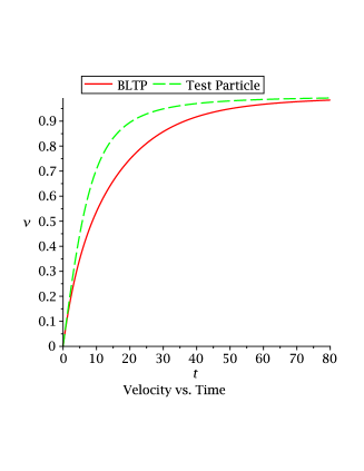
In Fig. 1 we show in units of as a function of in units of both for the test particle motion and for the BLTP motion with radiation-friction force given by (88). The applied electric field strength is in units of , which is a strong field for this problem. The radiation-friction effect is clearly visible.
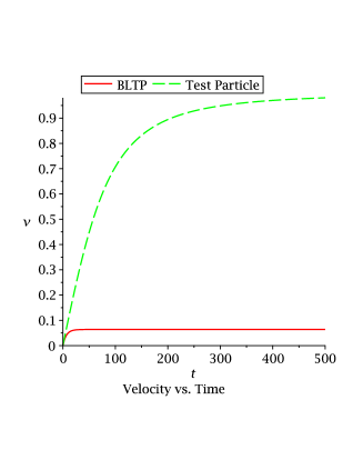
We note that for very weak applied field strength the radiation-reaction is captured by the “Newtonian-friction” approximation (89), and the point charge’s velocity will saturate at ; see Fig. 2 for an applied field strength of in units of .
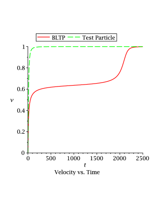
The sharp borderline between the “weak field” and “strong field” regimes determines a critical field strength for this problem. For field strengths just slightly above the critical value the velocity temporarily reaches a quasi-plateau, before it makes the final transition to approach the speed of light; see Fig. 3 for an applied field strength of in units of .
Although the term (88) is not an accurate formula for the radiation-reaction force in the physically interesting regime of very large values, it is entirely adequate for demonstrating that the radiation-reaction does not vanish identically in the BLTP version of this standard textbook-type problem. Moreover, we have treated the dynamics properly as a physical initial value problem with the same data as in the test particle formulation, unlike the treatment in Zayats where “the whole path traversed by the particle up to the present time contributes to [the self-force]” (quoted from Zayats ).
VIII Summary and Outlook
In this paper we have shown that a well-defined electromagnetic force on a point charge source of the classical electromagnetic field can be extracted from momentum balance among charges and field, whenever the electromagnetic vacuum law which supplies the closure relation for the pre-metric Maxwell field equations leads to a finite field momentum vector which is differentiable with respect to time.
For the BLTP law of the vacuum we even reported that we were able to prove, in collaboration with S. Tahvildar-Zadeh, that the BLTP electromagnetic force as defined in (16) furnishes a well-posed joint initial value problem for fields and point particles which is of second-order in the particle positions; see KTZonBLTP for the details. To the best of our knowledge BLTP electrodynamics is the first classical electrodynamical theory of point charges and their electromagnetic fields which has been shown to be dynamically well-posed, free of infinite “self” energies etc. and ill-defined Lorentz “self” forces, and free of the -problem. Incidentally, neither Bopp, Landé–Thomas, nor Podolsky considered the definition of the force given in this paper, but tried (in vain) to implement the ill-defined Lorentz force formula into their theory.
We have illustrated the well-posed BLTP electrodynamical initial value problem by revisiting the standard textbook problem of a point charge released from rest in a constant applied electrostatic field. Our discussion confirms that the test-particle approximation is valid in the initial dynamical phase, with radiation-reaction corrections first in form of a linear , “Newtonian friction”-type term (at least in the small regime), and eventually in a non-linear manner.
A most interesting finding, valid for arbitrary , is that in the initial phase of the dynamics the particle inertia is determined entirely by its bare rest mass, not by the mass of the (electromagnetically) “dressed” particle. The latter is generally thought to control the inertia in scattering scenarios. The predominance of scattering experiments, in particular in high energy physics, has led to the general belief that only the “dressed particle” mass is observable in experiments, not the bare mass. Our findings by contrast suggest that the bare mass may be observable by cleverly setting up an initial value problem in the laboratory.
True, BLTP electrodynamics may not be the most realistic classical theory, but it surely is a “proof of concept,” signaling that analogous results should be feasible also for putatively more realistic models, in particular the BI electrodynamics. We remark that a well-defined joint initial value problem for the MBI fields and their point charge sources was formulated with the help of a Hamilton–Jacobi-type theory in KieMBIinJSPa , but it is not clear whether that theory is well-posed, nor is it clear that its dynamics is independent of the invoked foliation of spacetime it needs for its formulation. Since the setup given in the present paper is truly Lorentz co-variant and foliation-independent, it should shed light on the formulation given in KieMBIinJSPa by comparing the two. Incidentally, neither Born & Infeld, nor Schrödinger, nor Dirac, proposed the electromagnetic force given in this paper but instead tried to implement the ill-defined Lorentz force formula into the Born–Infeld electrodynamics; cf. KieMBIinREGENSBURG .
Inside the family of well-posed classical models one may hope to find the classical limit of the elusive, mathematically well-defined and physically viable, special-relativistic quantum theory of electromagnetism.
Having obtained a rigorous control over the classical electromagnetic radiation-reaction problem, an important next goal in the realm of classical physics is to get a rigorous hand on the gravitational radiation-reaction problem. As a first step, armed with the insights gained from the special-relativistic theory of motion formulated in this paper we have embarked on an assessment of the Einstein–Infeld–Hoffmann EIH legacy; cf. KTZonEIHa .
Acknowledgment
The ideas and insights reported here evolved over many years, during which I have benefited especially from discussions with (in alphabetical order): Walter Appel, Holly Carley, Dirk Deckert, Detlef Dürr, Vu Hoang, Markus Kunze, Volker Perlick, Maria Radosz, Jared Speck, Herbert Spohn, and Shadi Tahvildar-Zadeh in particular, for which I am very grateful. After the first version of this paper was made public, the author received several comments which were implemented in the revision. Many thanks go: to Bob Wald for drawing attention to Ref. GHW ; to Mario Hubert for catching a sign error in the Born–Infeld section; to Herb Johnson for prompting me to explain the MBLTP initial value problem more clearly; to the referee for the helpful comments which improved the presentation, and for prompting me to work out the example discussed in section VII.
References
References
- (1) Lorentz, H.A., La théorie électromagnetique de Maxwell et son application aux corps mouvants, Arch. Néerl. Sci. Exactes Nat. 25, pp. 363–552 (1892).
- (2) Liénard, A., Champ électrique et magnétique produit par une charge concentrée en un point et animée d’un mouvement quelconque, L’ Éclairage électrique 16 p.5; ibid. p. 53; ibid. p. 106 (1898).
- (3) Wiechert, E., Elektrodynamische Elementargesetze, Arch. Néerl. Sci. Exactes Nat. 5, 549-573 (1900).
- (4) Jackson, J.D., Classical electrodynamics, J. Wiley & Sons, New York ed. (1975); ed. (1999).
- (5) Gralla, S.E., Harte, A., and Wald, R.M., A rigorous derivation of electromagnetic self-force, Phys. Rev. D 80:024031 (2009).
- (6) Lorentz, H.A., Weiterbildung der Maxwell’schen Theorie: Elektronentheorie., Encyklopädie d. Mathematischen Wissenschaften , Art. 14, pp. 145–280 (1904).
- (7) Yaghjian, A.D., “Relativistic dynamics of a charged sphere,” Lect. Notes Phys. m11, Springer, Berlin (1992).
- (8) Spohn, H., Dynamics of charged particles and their radiation fields, Cambridge UP (2004).
- (9) Appel, W., and Kiessling, M.K.-H., Mass and spin renormalization in Lorentz electrodynamics, Annals Phys. 289, 24–83 (2001).
- (10) Dirac, P. A. M., Classical theory of radiating electrons, Proc. Roy. Soc. A 167, 148–169 (1938).
- (11) Fermi, E., Über einen Widerspruch zwischen der elektrodynamischen und der relativistischen Theorie der elektromagnetischen Masse, Phys. Zeitschr. 23, 340-344 (1922).
- (12) Landau, L. D., and Lifshitz, E., The Classical Theory of Fields, Pergamon (1951).
- (13) Poisson, E., Pound, A., and Vega, I., The motion of point particles in curved spacetime, Living Rev. Rel. 14,7(190) (2011).
- (14) Burton, D.-A., and Noble, A., Aspects of electromagnetic radiation in strong fields, Contemp. Phys. 55, 110–121 (2014).
- (15) Ares de Parga, G., Mares, R., and Dominguez, S. An unphysical result for the Landau–Lifshitz equation of motion for a charged particle, Rev. Mex. Fis. 52, 139–142 (2006).
- (16) Deckert, D.-A., and Hartenstein, V., On the initial value formulation of classical electrodynamics J. Phys. A: Math. Theor. 49, 445202 (19pp.) (2016).
- (17) Miller, A. I., Albert Einstein’s special theory of relativity, Springer, New York (1998).
- (18) Abraham, M., Die Grundhypothesen der Elektronentheorie, Phys. Z. 5, 576-579 (1904).
- (19) Hehl, F. W., and Obukov, Y. N., “Foundations of Classical Electrodynamics,” Birkhäuser, Basel (2003).
- (20) Born, M., and Infeld, L., Foundation of the new field theory, Proc. Roy. Soc. London A 144, 425–451 (1934).
- (21) Białynicki-Birula, I., Nonlinear electrodynamics: Variations on a theme by Born and Infeld, pp. 31-48 in “Quantum theory of particles and fields,” eds. B. Jancewicz and J. Lukierski, World Scientific, Singapore (1983).
- (22) Bopp, F., Eine lineare Theorie des Elektrons, Annalen Phys. 430, 345–384 (1940).
- (23) Bopp, F., Lineare Theorie des Elektrons. II, Annalen Phys. 434, 573–608 (1943).
- (24) Landé, A., Finite Self-Energies in Radiation Theory. I, Phys. Rev. 60, 121–126 (1941).
- (25) Landé, A., and Thomas, L.H., Finite Self-Energies in Radiation Theory. II, Phys. Rev. 60, 514–523 (1941).
- (26) Podolsky, B., A generalized electrodynamics. Part I: Non-quantum, Phys. Rev. 62, 68–71 (1942).
- (27) Podolsky, B., and Schwed, P., A review of generalized electrodynamics, Rev. Mod. Phys. 20, 40–50 (1948).
- (28) Mie, G., Grundlagen einer Theorie der Materie, I, Annalen Phys. 37, 511-534 (1912).
- (29) Mie, G., Grundlagen einer Theorie der Materie, II, Annalen Phys. 39, 1-40 (1912).
- (30) Schwarzschild, K. Zur Elektrodynamik.I, Nachr. Ges. Wiss. Göttingen, 126–131 (1903).
- (31) Speck, J.R., The nonlinear stability of the trivial solution to the Maxwell-Born-Infeld system, J. Math. Phys. 53, 083703(83pp) (2012).
- (32) Serre, D., Les ondes planes en éctromagnététisme non-linéaire, Physica D 31, 227-251 (1988).
- (33) Brenier, Y., Hydrodynamic structure of the augmented Born–Infeld equations, Arch. Rat. Mech. Anal. 172, 65-91 (2004).
- (34) Kiessling, M.K.-H., On the quasi-linear elliptic PDE in physics and geometry, Commun. Math. Phys. 314, 509–523 (2012); Correction ibid. 364, 825–833 (2018).
- (35) Carley, H. K., Kiessling, M. K.-H., and Perlick, V., On the Schrödinger spectrum of a hydrogen atom with BLTP interactions between electron and proton, Int. J. Mod. Phys. A 34, 1950146 (2019).
- (36) Kiessling, M.K.-H., and Tahvildar-Zadeh, A. S., Bopp-Landé-Thomas-Podolsky electrodynamics as initial value problem, in preparation (2020).
- (37) Kiessling, M.K.-H., and Tahvildar-Zadeh, A. S., The Einstein–Infeld–Hoffmann legacy in mathematical relativity. I: The classical motion of charged point particles, 16pp. in Proc. of the 15th Marcel Grossmann Meeting on General Relativity, Rome, Italy (2018); Int. J. Mod. Phys. D 28 1930017 (2019).
- (38) Gratus, J., Perlick, V., and Tucker, R.W., On the self-force in Bopp–Podolsky electrodynamics, J. Phys. A: Math. Theor. 48, 435401 (28pp.) (2015).
- (39) Zayats, A.E., Self-interaction in the Bopp-Podolsky electrodynamics: Can the observable mass of a charged particle depend on its acceleration?, Annals Phys. (NY)342, 11–20 (2014).
- (40) Hoang, V., and Radosz, M., On the self-force in higher-order electrodynamics, Preprint (41pp.) arXiv:1902.06386 (2019).
- (41) Quinn, T.C., and Wald, R.M., An axiomatic approach to electromagnetic and gravitational radiation reaction of particles in curved spacetime, Phys. Rev. D 56, 3381–3394 (1997).
- (42) Kijowski, J., Electrodynamics of moving particles, Gen. Rel. Grav. 26, 167-192 (1994).
- (43) Detweiler, S., and Whiting, B. F., Self-force via a Green’s function decomposition, Phys. Rev. D 67, 024025 (2003).
- (44) Feynman, R. P., A relativistic cut-off for classical electrodynamics, Phys. Rev. 74, 939–946 (1948).
- (45) Einstein, A., Infeld, L., and Hoffmann, B., The gravitational equations and the problem of motion, Annals Math. 39, 65-100 (1938).
- (46) Kiessling, M.K.-H., Electromagnetic field theory without divergence problems. 1. The Born legacy, J. Stat. Phys. 116, 1057-1122 (2004).
- (47) Kiessling, M.K.-H., On the Motion of Point Defects in Relativistic Fields, pp.299–335 in: Finster F., Müller O., Nardmann M., Tolksdorf J., Zeidler E. (eds) “Quantum Field Theory and Gravity.” Springer, Basel (2012).