T-Branes, String Junctions, and 6D SCFTs

Abstract

Recent work on 6D superconformal field theories (SCFTs) has established an intricate correspondence between certain Higgs branch deformations and nilpotent orbits of flavor symmetry algebras associated with T-branes. In this paper, we return to the stringy origin of these theories and show that many aspects of these deformations can be understood in terms of simple combinatorial data associated with multi-pronged strings stretched between stacks of intersecting $7$-branes in F-theory. This data lets us determine the full structure of the nilpotent cone for each semi-simple flavor symmetry algebra, and it further allows us to characterize symmetry breaking patterns in quiver-like theories with classical gauge groups. An especially helpful feature of this analysis is that it extends to “short quivers” in which the breaking patterns from different flavor symmetry factors are correlated.

1 Introduction

One of the surprises from string theory is the prediction of whole new classes of quantum field theories decoupled from gravity. Central examples of this sort are 6D superconformal field theories (SCFTs). The only known way to reliably engineer examples of such theories is to start with a background geometry in string / M- / F-theory, and to consider a singular limit in which all length scales are sent to zero or infinity (for early work in this direction see e.g. [1, 2, 3]). Since small deformations away from these scaling limits have a sensible coupling to higher-dimensional gravity, there is strong evidence that this leads to an interacting conformal fixed point.

The most flexible method known for constructing such theories is via F-theory on a non-compact, elliptically-fibered Calabi-Yau threefold. SCFTs are generated by simultaneously contracting a configuration of curves in the base geometry. There is now a classification of all elliptic threefolds which can generate a 6D SCFT, and in fact, each known 6D SCFT can be associated with some such threefold [4, 5] (see also [6, 7]). For a recent review, see reference [11].

In these sorts of constructions, one begins away from the fixed point of interest and then tunes to zero various operator vevs in the low energy effective field theory. In this UV limit, the effective field theory description breaks down, but the stringy description still remains well-behaved. From this perspective, the main question is to better understand the microscopic structure of these 6D SCFTs.

The F-theory realization of 6D SCFTs provides insight into the corresponding structure of these theories as well as their moduli spaces (see [11]). Perhaps surprisingly, all known 6D SCFTs resemble generalizations of quiver gauge theories in which (on a partial tensor branch) the theory involves ADE gauge groups linked together by 6D conformal matter [12, 13]. The topology of these quivers is rather simple, and consists of a single spine of such gauge groups. The space of tensor branch deformations translates in the geometry to the moduli space of volumes for the contractible curves in the base of the elliptic threefolds. Additionally, Higgs branch deformations translate to complex structure deformations of the corresponding elliptic threefolds.

The quiver-like description of 6D SCFTs also suggests that Higgs branch deformations can be understood in terms of breaking patterns associated with the flavor symmetries of these theories. For example, in the $7$-brane gauge theory, nilpotent elements of the flavor symmetry algebra correspond to “T-brane configurations” of $7$-branes. For a partial list of references to the T-brane literature, see references [14, 15, 16, 17, 18, 19, 20, 21, 22, 23, 24, 25, 26, 27, 28, 29, 30, 31, 32, 33, 34, 35, 36].

A pleasant aspect of nilpotent elements is that they come equipped with a partial ordering, as dictated by the symmetry breaking pattern in the original UV theory. Indeed, the orbit of each nilpotent element under the adjoint action specifies (under Zariski closure) a partially ordered set. This partial ordering determines fine-grained structure for Higgs branch flows between different 6D SCFTs [22, 37] and points the way to a possible classification of RG flows between 6D SCFTs [30].

This has been established in the case of 6D SCFTs with a sufficient number of gauge group factors in the quiver-like description, i.e., “long quivers,” where Higgsing of the different flavor symmetries is uncorrelated, and there are also hints that it extends to the case of “short quivers” in which the structure of Higgsing is correlated.

One feature which is somewhat obscure in this characterization of Higgs branch flows is the actual breaking pattern taking place in the quiver-like gauge theory. Indeed, in the case of a weakly-coupled quiver gauge theory, the appearance of matter transforming in representations of different gauge groups means that the corresponding D-flatness conditions for one vector multiplet will automatically be correlated with those of neighboring gauge group nodes. This means that each breaking pattern defined on the exterior of a quiver will necessarily propagate towards the interior of the quiver. Even in the case of quiver gauge theories with classical algebras, the resulting combinatorics for tracking the breaking pattern of a Higgs branch deformation can be quite intricate.

To address these issues, in this paper we use the physics of brane recombination to extract the combinatorics of Higgs branch flows in 6D SCFTs. In stringy terms, brane recombination is associated with the condensation of strings stretched between different branes. In the context of F-theory, strings can be bound states of F1- and D1- strings, and they can have multiple ends. Our task, then, will be to show how such multi-pronged strings attach between different stacks of branes, and moreover, how this leads to a natural characterization of brane recombination for Higgs branch flows in 6D SCFTs.

Since we will be primarily interested in flows driven by nilpotent orbits, we first spell out how a given configuration of multi-pronged strings attached to bound states of $[p,q]$ $7$-branes maps on to the breaking pattern associated with a particular nilpotent orbit of an algebra. Separating these branes from one another corresponds to a choice of Cartan subalgebra, and strings stretched between these separated branes correspond to Lie algebra elements associated with roots of the Lie algebra, defining a directed graph between the nodes spanned by these branes. In particular, we show that we can always generate a nilpotent element of the (complexified) Lie algebra by working in terms of a directed graph which points in one direction. We also show that, starting from such a directed graph, appending additional strings always leads to a nilpotent element with a strictly larger nilpotent orbit. We thus construct the entire nilpotent cone of each Lie algebra of type ABCDEFG using such multi-pronged string junctions.

With this result in place, we next turn to an analysis of Higgs branch flows in quiver-like 6D SCFTs, as generated by T-brane deformations. We primarily focus on 6D SCFTs generated by M5-branes probing an ADE singularity with flavor symmetry $G_{ADE}\times G_{ADE}$, as well as tensor branch deformations of these cases to non-simply laced flavor symmetry algebras. As found in [30], these are progenitor theories for many 6D SCFTs (the other being E-string probes of ADE singularities [13, 5, 39, 40, 41]). The partial tensor branch of these parent UV theories are all of the form:

$$[G_{0}]-G_{1}-...-G_{k}-[G_{k+1}]$$ (1.1)

with $G_{0},G_{k+1}$ flavor symmetries and $G_{1},...,G_{k}$ gauge symmetries. We show that Higgs branch flows are determined by a system of coupled D-term constraints, one for each node of such a quiver gauge theory. This in turn means that the “links” between gauge nodes behave as a generalization of matter, as suggested by the structure of these quivers. We also show that condensing these strings leads to a sequence of brane recombinations, relying on a parallel with Hanany-Witten moves [68] seen in the type IIA framework to derive the type IIB recombination moves. We present a complete characterization of quiver-like theories with classical algebras, and briefly discuss what would be needed to extend this analysis to quiver-like theories with exceptional gauge group factors.

The explicit characterization of nilpotent orbits in terms of string junctions also allows us to study Higgs branch flows in which the number of gauge groups is small. This case is especially interesting because there are non-trivial correlations on the symmetry breaking patterns, one emanating from the left flavor symmetry $G_{0}$ and the subsequent D-term constraints on its gauged neighbors and one emanating from the right flavor symmetry $G_{k+1}$ and its gauged neighbors in the quiver of line (1.1). This sort of phenomenon occurs whenever the size of the nilpotent orbit of the flavor algebras is sufficiently large, and the number of gauge groups $k$ is sufficiently small. We study these “overlapping T-branes” in detail in the case of the classical algebras. In particular, we show how to extract the resulting IR SCFT using our picture in terms of brane recombination. We leave the case of short quivers with exceptional gauge groups / flavor symmetries to future work.

The rest of this paper is organized as follows. First, in section 2, we review in general terms the structure of 6D SCFTs as quiver-like gauge theories, and we explain how the worldvolume theory on $7$-branes leads to a direct link between Higgs branch flows and nilpotent orbits of flavor symmetries. In section 3, we show how to reconstruct the nilpotent cone of a flavor symmetry algebra in terms of the combinatorial data of strings stretched between stacks of $[p,q]$ $7$-branes. Section 4 uses this combinatorial data to provide a systematic method for analyzing Higgs branch flows in quiver-like theories with classical gauge groups, including cases with 6D conformal matter. In section 5, we study Higgs branch flows from overlapping nilpotent orbits in short quivers, and in section 6 we present our conclusions. A number of additional detailed computations are included in the Appendices.

2 6D SCFTs as Quiver-Like Gauge Theories

In this section, we briefly review the relevant aspects of 6D SCFTs which we shall be studying in the remainder of this paper. The main item of interest for us will be the quiver-like structure of all such theories, and the corresponding Higgs branch flows associated with nilpotent orbits of the flavor symmetry algebra.

To begin, we recall that the F-theory realization of 6D SCFTs involves specifying a non-compact elliptically-fibered Calabi-Yau threefold $X\rightarrow B$, where the base $B$ of the elliptic fibration is a non-compact Kähler surface. In minimal Weierstrass form, these elliptic threefolds can be viewed as a hypersurface:

$$y^{2}=x^{3}+fx+g.$$ (2.1)

The order of vanishing for the coefficients $f$, $g$ and the discriminant $\Delta=4f^{3}+27g^{2}$ dictate the structure of possible gauge groups, flavor symmetries and matter content in the 6D effective field theory. We are particularly interested in the construction of 6D SCFTs, which requires us to simultaneously collapse a collection of curves in the base to zero size at finite distance in the Calabi-Yau metric moduli space. This can occur for curves with negative self-intersection, and compatibility with the condition that we maintain an elliptic fibration over generic points of each curve imposes further restrictions [4]. Each such configuration can be viewed as being built up from intersections of non-Higgsable clusters (NHCs) [42] and possible enhancements in the singularity type over each such curve. The tensor branch of the 6D SCFT corresponds to resolving the collapsing curves in the base to finite size, and the Higgs branch of the 6D SCFT corresponds to blow-downs and smoothing deformations of the Weierstrass model such as [43]:

$$y^{2}=x^{3}+(f+\delta f)x+(g+\delta g).$$ (2.2)

In references [4, 5], the full list of possible F-theory geometries which could support a 6D SCFT was determined. Quite remarkably, all of these theories have the structure of a quiver-like gauge theory with a single spine of gauge group nodes and only small amounts of decoration by (generalized) matter on the left and right of each quiver. In this description, $7$-branes with ADE gauge groups intersect at points where additional curves have collapsed. These points are often referred to as “conformal matter” since they localize at points just as in the case of ordinary matter in F-theory [12, 13]. These configurations indicate the presence of additional operators in the 6D SCFT and, like ordinary matter, can have non-trivial vevs, leading to a deformation onto the Higgs branch. A streamlined approach to understanding the vast majority of 6D SCFTs was obtained in [30] where it was found that any 6D SCFT can be viewed as “fission products,” namely as deformations of a quiver-like theory with partial tensor branch such as:

$$[E_{8}]\overset{\mathfrak{g}_{ADE}}{1}\overset{\mathfrak{g}_{ADE}}{2}...\overset{\mathfrak{g}_{ADE}}{2}[G_{ADE}]$$ (2.3)

or:

$$[G_{ADE}]\overset{\mathfrak{g}_{ADE}}{2}...\overset{\mathfrak{g}_{ADE}}{2}[G_{ADE}],$$ (2.4)

where the few SCFTs which cannot be understood in this way can be obtained by adding a tensor multiplet and weakly gauging a common flavor symmetry of these fission products through a process known as fusion. In the above, each compact curve of self-intersection $-n$ with a $7$-brane gauge group of ADE type is denoted as $\overset{\mathfrak{g}_{ADE}}{n}$. The full tensor branch of these theories is obtained by performing further blowups at the collision points between the compact curves (in the D- and E-type cases). To emphasize this quiver-like structure, we shall often write:

$$[G_{0}]-G_{1}-...G_{k}-[G_{k+1}],$$ (2.5)

to emphasize that there are two flavor symmetry factors (indicated by square brackets), and the rest are gauge symmetries.

The 6D SCFTs given by lines (2.3) and (2.4) can also be realized in M-theory. The theories of line (2.3) arise from an M5-brane probing an ADE singularity which is wrapped by an $E_{8}$ nine-brane. The theories of line (2.4) arise from M5-branes probing an ADE singularity. In what follows, we shall primarily be interested in understanding Higgs branch flows associated with the theories of line (2.4).

For $G_{ADE}$ of A or D type, the IR SCFTs of these Higgs branch flows can also be realized in type IIA. $SU$ gauge algebras are obtained from the worldvolume of D6-branes suspended between spacetime-filling NS5-branes, while $SO$ algebras and $Sp$ gauge algebras also require $O6^{-}$ and $O6^{+}$ branes, respectively, stretched between $\frac{1}{2}$ NS5-branes. These constructions will prove especially useful in section 4, where we discuss Hanany-Witten moves of the branes of the type IIA construction.

One of the main ways to cross-check the structure of proposed RG flows is through anomaly matching constraints. The anomaly polynomial of a 6D SCFT is calculable because the tensor branch description of each such theory is available from the F-theory description, and the anomaly polynomial obtained on this branch of moduli space can be matched to that of the conformal fixed point [44, 45, 43, 46, 47]. To fix conventions, we often write this as a formal eight-form with conventions (as in reference [11]):

$$I_{8} =\alpha c_{2}(R)^{2}+\beta c_{2}(R)p_{1}(T)+\gamma p_{1}(T)^{2}+\delta p_{2}(T)$$

$$+\sum_{i}\left[\mu_{i}\,\mathrm{Tr}F_{i}^{4}+\,\mathrm{Tr}F_{i}^{2}\left(\rho_{i}p_{1}(T)+\sigma_{i}c_{2}(R)+\sum_{j}\eta_{ij}\,\mathrm{Tr}F_{j}^{2}\right)\right],$$ (2.6)

where in the above, $c_{2}(R)$ is the second Chern class of the $SU(2)_{R}$ symmetry, $p_{1}(T)$ is the first Pontryagin class of the tangent bundle, $p_{2}(T)$ is the second Pontryagin class of the tangent bundle, and $F_{i}$ is the field strength of the $i^{th}$ symmetry, where $i$ and $j$ run over the flavor symmetries of the theory. See the review article [11] as well as the Appendices for additional details on how to calculate the anomaly polynomial in specific 6D SCFTs.

Returning to the F-theory realization of the 6D SCFTs of line (2.4), there is a large class of Higgs branch deformations associated with nilpotent orbits of the flavor symmetry algebras. Moreover, nilpotent elements admit a partial ordering which also dictates a partial ordering of 6D fixed points. We say that a nilpotent element $\mu\preceq\nu$ when there is an inclusion of the orbits under the adjoint action: Orbit$(\mu)\subseteq$ $\overline{\text{Orbit}(\nu)}$.

In the 6D SCFT, there is a triplet of adjoint valued moment maps $D_{\text{adj}}^{1},$ $D_{\text{adj}}^{2},$ $D_{\text{adj}}^{3}$ which couple to the flavor symmetry current supermultiplet. The nilpotent element can be identified with the complexified combination $D_{\text{adj}}^{\mathbb{C}}=D_{\text{adj}}^{1}+iD_{\text{adj}}^{2}$. Closely related to this triplet of moment maps are the triplet of D-term constraints for each gauge group factor $G_{j}$ for $j=1,...,k$. Labeling these as a three-component vector taking values in the adjoint of each such group $\overrightarrow{D}_{j}$, supersymmetric vacua are specified in part by the conditions:

$$\overrightarrow{D}_{j}=0\text{ for all }j,$$ (2.7)

modulo unitary gauge transformations. We note that in the weakly coupled context, the D-term constraints for each gauge group factor are in fact correlated with one another. In particular, if we specify a choice of moment map $\overrightarrow{D}_{0}\neq 0$ and $\overrightarrow{D}_{k+1}\neq 0$ on the left and right of the quiver, respectively, this propagates to a non-trivial breaking pattern in the interior of the quiver.

That being said, the actual description of this breaking pattern using 6D conformal matter is poorly understood because there is no weakly coupled description available for these degrees of freedom. So, while we expect there to be a correlated breaking pattern for gauge groups in the interior of a quiver, the precise structure of these terms is unclear due to the unknown structure of the microscopic degrees of freedom in the field theory.

In spite of this, it is often possible to extract the resulting IR fixed point after such a deformation, even in the absence of a Lagrangian description. The main reason this is possible is because in the context of an F-theory compactification, we already have a classification of all possible outcomes which could have resulted from a Higgs branch flow (since we have a classification of 6D SCFTs). In many cases, this leads to a unique candidate theory after Higgsing, and this has been used to directly determine the Higgsed theory. Even so, this derivation of the theory obtained after Higgsing involves a number of steps which are not entirely systematic, thus leading to potential ambiguities in cases where the number of gauge group factors in the quiver is sufficiently small that there is a non-trivial correlation in the symmetry breaking pattern obtained from a pair of nilpotent orbits (one on the left and one on the right of the quiver). We refer to such quivers as being “short,” and the case where there is no correlation between breaking patterns from different nilpotent orbits as “long.”

One of our aims in the present paper will be to determine the condensation of strings stretched between different stacks of branes. Our general strategy for analyzing Higgs branch flows will therefore split into two parts:

• First, we determine the particular configuration of multi-pronged strings associated with each nilpotent orbit.

• Second, we determine how to consistently condense these multi-pronged string states to trigger brane recombination in the quiver-like gauge theory.

3 Nilpotent Orbits from String Junctions

One of our aims in this paper is to better understand the combinatorial structure associated with symmetry breaking patterns for 6D SCFTs. In this section we show how to construct all of the nilpotent orbits of a semi-simple Lie algebra of type ABCDEFG from the structure of multi-pronged string junctions. The general idea follows earlier work on the construction of such algebras, as in [48, 49, 50] (see also [51, 52, 53]). We refer the interested reader to Appendix A for additional details and terminology on nilpotent orbits which we shall reference throughout this paper.

Recall that in type IIB, we engineer such algebras using $[p,q]$ $7$-branes, namely a bound state of $p$ D7-branes and $q$ S-dual $7$-branes. Labeling the monodromy of the axio-dilaton around a source of $7$-branes by a general element of $SL(2,\mathbb{Z})$:

$$\tau\mapsto\frac{a\tau+b}{c\tau+d}\text{ \ \ for \ \ }\left[\begin{array}[c]{cc}a&b\\ c&d\end{array}\right]\in SL(2,\mathbb{Z})\text{,}$$ (3.1)

a $[p,q]$ $7$-brane determines a conjugacy class in $SL(2,\mathbb{Z})$ as specified by the orbit of:

$$M_{[p,q]}=\left[\begin{array}[c]{cc}1+pq&-p^{2}\\ q^{2}&1-pq\end{array}\right].$$ (3.2)

The relevant structure for realizing the different ADE algebras are the monodromies:

$$A=M_{[1,0]}=\left[\begin{array}[c]{cc}1&-1\\ 0&1\end{array}\right]\text{, \ \ }B=M_{[1,-1]}=\left[\begin{array}[c]{cc}0&-1\\ 1&2\end{array}\right]\text{, \ \ }$$ (3.7)

$$C=M_{[1,1]}=\left[\begin{array}[c]{cc}2&-1\\ 1&0\end{array}\right]\text{, \ \ }X=M_{[2,-1]}=\left[\begin{array}[c]{cc}-1&-4\\ 1&3\end{array}\right].$$ (3.12)

The $7$-branes necessary to engineer various Lie algebras follow directly from the Kodaira classification of possible singular elliptic fibers at real codimension two in the base of an F-theory model [54, 55, 56]. They can also be directly related to a set of basic building blocks in the string junction picture worked out in [48] which we label as in reference [57]:

$$A_{N} :A^{N+1}$$ (3.13)

$$H_{N} :A^{N+1}C\text{ \ \ (for }N=0,1,2\text{)}$$ (3.14)

$$D_{N} :A^{N}BC$$ (3.15)

$$E_{N} :A^{N-1}BC^{2}\text{ \ \ (for }N=6,7,8\text{)}$$ (3.16)

$$\widetilde{E}_{N} :A^{N}XC\text{ \ \ (for }N=6,7,8\text{)}.$$ (3.17)

The $H_{N}$ series in the second line represents an alternative way to realize low rank $SU$ type algebras. We also note that in the case of the A- and D- series, it is possible to remain at weak string coupling, while the H- and E-series require order one values for the string coupling. Here, we have indicated two alternate presentations of the $E$-type algebras (see reference [57]). It will prove convenient in what follows to use the $\widetilde{E}_{N}$ realization with an $X$-brane. The non-simply laced algebras have the same $SL(2,\mathbb{Z})$ monodromy type. In the string junction description, this involves further identifications of some of the generators of the algebra by a suitable outer automorphism. Some aspects of this case are discussed in [50].

We would like to understand the specific way that nilpotent generators of the Lie algebra are encoded in this physical description. In all these cases, the main idea is to first separate the $7$-branes so that we have a physical realization of the Cartan subalgebra. Then, a string which stretches from one brane to another will correspond to an 8D vector boson with mass dictated by the length of the path taken to go from one stack to the other:

$$\text{mass}\sim\frac{\text{length}}{\ell_{\ast}^{2}},$$ (3.18)

with $\ell_{\ast}$ a short distance cutoff. In the limit where all the $7$-branes are coincident, we get a massless state.

With this in mind, let us recall how we engineer the gauge algebra $\mathfrak{su}(N)$ using D7-branes. All we are required to do in this case is introduce $N$ D7-branes, which are $[p,q]$ $7$-branes with $p=1$ and $q=0$. Labeling the $7$-branes as $A_{1},...,A_{N}$, we can consider an open string which stretches from brane $A_{i}$ to brane $A_{j}$. Since this string comes with an orientation, we can write:

$$A_{i}\rightarrow A_{j}\text{,}$$ (3.19)

and introduce a corresponding nilpotent $N\times N$ matrix with a single entry in the $i^{th}$ row and $j^{th}$ column. We denote by $E_{i,j}$ the matrix with a one in this single entry so that the corresponding nilpotent element is written as $v_{i,j}E_{i,j}$ with no summation on indices. Conjugation by an $SL(n,\mathbb{C})$ element reveals that the actual entry does not affect the orbit. We will, however, be interested in RG flows generated by adding perturbations away from a single entry, so we will often view $v_{i,j}$ as indicating a vev / energy scale. In this manner, we can represent an RG flow triggered by moving onto the Higgs branch of the theory, which is labeled by a nilpotent orbit of a Lie algebra, in terms of a collection of strings stretched between the $7$-branes.

	Dynkin diagram	IIB with mirror plane	Physical picture from [49]	Branching rule to $\mathfrak{su}(4)\times\mathfrak{u}(1)$	Positive roots
$A_{4}$				$24\rightarrow 15_{0}+4_{1}+\overline{4}_{\scalebox{0.75}[1.0]{-}1}+1_{0}$	10 one-pronged strings: $a_{i}-a_{j}$
$B_{4}$				$36\rightarrow 15_{0}+6_{2}+\overline{6}_{\scalebox{0.75}[1.0]{-}2}+4_{1}+\overline{4}_{\scalebox{0.75}[1.0]{-}1}+1_{0}$	10 one-pronged strings: $a_{i}-a_{j},\ \tilde{a}_{j}-\tilde{a}_{i}$ 6 two-pronged strings: $a_{i}-\tilde{a}_{j},\ a_{j}-\tilde{a}_{i}$
$C_{4}$				$36\rightarrow 10_{2}+\overline{10}_{\scalebox{0.75}[1.0]{-}2}+15_{0}+1_{0}$	6 one-pronged strings: $a_{i}-a_{j},\ \tilde{a}_{j}-\tilde{a}_{i}$ 4 double strings: $a_{i}-\tilde{a}_{i}$ 6 two-pronged strings: $a_{i}-\tilde{a}_{j},\ a_{j}-\tilde{a}_{i}$
$D_{4}$				$28\rightarrow 6_{2}+\overline{6}_{\scalebox{0.75}[1.0]{-}2}+15_{0}+1_{0}$	6 one-pronged strings: $a_{i}-a_{j},\ \tilde{a}_{j}-\tilde{a}_{i}$ 6 two-pronged strings: $a_{i}-\tilde{a}_{j},\ a_{j}-\tilde{a}_{i}$

Table 1: Summary of basic properties for the string junction realization of the classical Lie algebras $A_{4}$, $B_{4}$, $C_{4}$, $D_{4}$. The columns from left to right are: Dynkin diagrams, IIB brane picture, string junction picture from [49], branching rule of adjoint decomposition in $\mathfrak{su}(4)\times\mathfrak{u}(1)$, explicit expression of groups of positive roots based on the adjoint decomposition. Here the indices $i$, $j$ run from $1$ to the number of nodes on the left-hand side of the mirror ($BC$). The tilde nodes are the reflected branes and the indices continue running as $\tilde{i}=N-i$ where $N$ is the total number of nodes in the diagram.

Figure 1: Separating a collection of A-type branes leads to a deformation of $\mathfrak{su}(N)$ to the Cartan subalgebra. Open strings stretched between distinct branes are associated with specific generators in the complexified Lie algebra. In the figure, this is shown for a string stretched from brane $A_{i}$ to brane $A_{j}$.

Ordering the branes $A_{1},..,A_{N}$ from left to right in the plane transverse to the stack of $7$-branes, we see that we can now populate the strictly upper triangular portion of a matrix in terms of strings $A_{i}\rightarrow A_{j}$ for $i<j$ (see figure 1). So in other words, we can populate all possible nilpotent orbits (in this particular basis). Similar considerations hold for the other algebras, but clearly, this depends on a number of additional features such as unoriented open strings (in the case of the classical SO / Sp algebras) and multi-pronged string junctions (in the case of the exceptional algebras). A related comment is that we are just constructing a representative nilpotent element in the orbit of the Lie algebra. What we will show is that for any deformation onto the Cartan, there is a “minimal length” choice, and all the other elements of the orbit are obtained through the adjoint action of the Lie algebra.

Our plan in the rest of this section will be to establish in detail how to construct the corresponding nilpotent orbits for each configuration of strings. Additionally, we show that not only can we generate all orbits, but that the combinatorial method of “adding extra strings” automatically generates a partial ordering on the space of nilpotent orbits, which reproduces the standard partial ordering of the nilpotent cone. The essential information for the classical Lie algebras, and in particular the list of simple and positive roots, is illustrated in table 1. We elaborate on the content of this table (as well the exceptional analogs) in the following subsections.

3.1 $SU(N)$: Partition by Grouping Branes with Strings

In the case of an $SU(N)$ flavor we simply have $N$ perturbative $A$-branes with $[p,q]=[1,0]$ charges. The $N-1$ simple roots of $SU(N)$ can be represented by strings joining two adjacent $A$-branes as shown in figure 2. We refer to these as “simple strings” due to their correspondence to the simple roots. The remaining (non-simple) roots are then described by strings connecting any two $A$-branes. The positive roots are represented by strings stretching from left to right while the negative ones would go in the opposite direction (as indicated by the arrows). That is we choose a basis for the generators of the $\mathfrak{su}_{N}$ algebra to be given by:

• $N(N-1)/2$ nilpositive elements $E_{i,j}$ with $1\leq i<j\leq N$ corresponding to strings stretching from the $i^{th}$ to the $j^{th}$ $A$-brane (with the arrow pointing from left to right).

• $N(N-1)/2$ nilnegative elements $E_{j,i}=X_{k}^{T}$ with $1\leq i<j\leq N$ corresponding to strings stretching from the $j^{th}$ to the $i^{th}$ $A$-brane (with the arrow now pointing from right to left).

• $(N-1)$ Cartans $[E_{i,i+1},E_{i+1,i}]$ for $1\leq i\leq N-1$.

Through out this paper we denote $E_{i,j}$ to be matrix with value $+1$ in the entry $(i,j)$ but zeros everywhere else. The positive simple roots are given by $\alpha_{i}$ $(1\leq i\leq rank(G))$, with the corresponding matrix representation labelled $E_{\alpha_{i}}$. Any non-simple root can then be labelled explicitly in terms of its simple roots constituents: $\alpha_{i,j,k,\dots,p,q}=\alpha_{i}+\alpha_{j}+\alpha_{k}+\dots+\alpha_{p}+\alpha_{q}$ and the corresponding matrix representation is obtained from nested commutators.

In this basis, the simple positive roots are $E_{i,i+1}$ for $1\leq i\leq N-1$, as illustrated by their corresponding directed strings in figure 2. Furthermore, we use the convention of [49] to keep track of the different monodromies. Namely, we only display the directions transverse to the $7$-brane, thus representing each $7$-brane as a point. In this picture the associated branch cut for $SL(2,\mathbb{Z})$ monodromy stretches vertically downward to infinity. This will not enter our analysis in any material way so in order not to overcrowd the figures, we will mostly not draw the branch cuts.

Figure 2: Brane diagram of strings/roots stretching between the $A$-branes yielding an $SU(N)$ flavor symmetry (see [49]). The dashed lines represent the position of branch cuts. Since they do not contribute to our analysis, they are not drawn in subsequent pictures.

We have already seen that nilpotent orbits of $SU(N)$ are parametrized by partitions of $N$ (with no restriction whatsoever). Thus it becomes natural to classify nilpotent orbits by how branes are grouped together. Namely, we can group any set of $A$-branes by stretching strings between them, giving rise to a particular partition of the $N$ branes. This partition is then in one-to-one correspondence with its corresponding nilpotent orbit. As an equivalence class, we have many different string configurations belonging to the same orbit (just like many different matrices have the same Jordan block decomposition). For instance, the three string junctions of figure 3 all represent the same $[3,2,1]$ partition:

• The first string junction picture has a matrix representation $M_{1}=E_{1,2}+E_{2,3}+E_{4,5}$.

• The second configuration has matrix representation $M_{2}=E_{1,3}+E_{3,6}+E_{4,5}$.

• And finally, the third one has matrix representation $M_{3}=E_{1,3}+E_{4,5}+E_{5,6}$.

Figure 3: Three equivalent ways of describing the partition $[3,2,1]$ in the set of nilpotent orbits of $SU(6)$. To each picture is associated a different matrix, but they all have the same Jordan block decomposition and thus belong to the same equivalence class.

To each nilpotent orbit of $SU(N)$ we can then associate one of many possible string junction pictures. To keep the picture as simple as possible, we choose to use only “simple” positive strings, that is strings stretching from left to right between two adjacent $A$-branes. This ensures that we only make use of simple roots. This typically does not completely fix a string junction representative, so we are free to make a convenient choice of the remaining possibilities.

By starting with a configuration with no string attached (a $[1^{N}]$ partition) we can add more and more strings to go from the $[2,1^{N-2}]$ orbit all the way to the $[N]$ partition. This generates a whole Hasse diagram of nilpotent orbits which exactly matches that which is mathematically predicted. Figure 4 illustrates this diagram for the case of $SU(6)$ where we associate a “standard” string junction picture to each nilpotent orbit according to how the branes are partitioned as we add more and more strings.

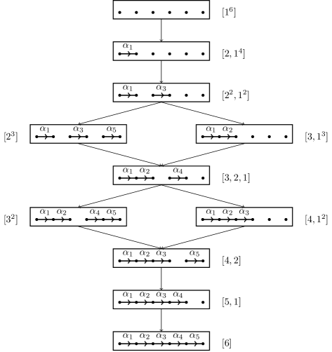
Figure 4: Hasse diagram of $SU(6)$ nilpotent deformations going from top (UV) to bottom (IR) where all simple roots are turned on and all corresponding “simple strings” connect the $A$-branes.

More precisely, in order to flow from one point of the Hasse diagram to the next, one simply needs to add a small perturbation, that is, an oriented string (moving from left to right) corresponding to a positive root. By the definition of the partial ordering of nilpotent orbits, this guarantees that the RG flow indeed always takes us deeper into the IR. Weyl transformations / brane permutations can then be used to reduce the obtained diagram back to one of the standard ones which only relies on the simple roots.

The flows involving only the addition of a simple root (corresponding to linking two more branes together) are fairly clear. The only cases where that is not so obvious are the ones corresponding to flows that are similar to the one described in figure 4 by going from $[2^{2},1^{2}]$ to $[3,1^{3}]$. For this we can add the string $\alpha_{2}+\alpha_{3}=a_{2}-a_{4}$, corresponding to a small deformation $\epsilon\cdot E_{2,4}$. This particular flow is illustrated in figure 5. Generalizing this procedure to arbitrary $SU(N)$ shows that the intermediate RG flows are guaranteed to be physically realizable in the same fashion.

$\Downarrow$

$\Leftrightarrow$    

Figure 5: One way of flowing from the $[2^{2},1^{2}]$ nilpotent orbit (top) to the $[3,1^{3}]$ orbit (bottom). In the top figure we have the matrix representation $M_{1}=E_{1,2}+E_{3,4}$. The flow is then induced by adding an extra string stretching between the $2^{nd}$ and $3^{rd}$ branes, as illustrated in the bottom left figure. This corresponds to the matrix $M_{2}=E_{1,2}+E_{3,4}+\epsilon\cdot E_{2,4}$. This matrix is similar to $M_{2}^{\prime}=E_{1,2}+E_{2,3}$ corresponding to the bottom right diagram. Thus, both bottom string junctions belong to the same nilpotent orbit $[3,1^{3}]$.

3.2 $SO(2N)$ and $SO(2N-1)$

In F-theory, the $SO(2N)$ and $SO(2N-1)$ geometries are realized by the presence of $A^{N}BC$-branes. In type IIB however, the $BC$-branes turn into an $O7^{-}$ orientifold plane (as discussed in [58]) which we refer here as the “BC-mirror”. This mirror reflects the $N$ $A$-branes across, yielding a total of $2N$ branes (half of which are physical, half of which are “image” branes). We thus represent $SO(2N)$ by $2N$ dots separated by a vertical line representing the $BC$-mirror, and $SO(2N-1)$ by merging one $A$-brane with its mirror image onto the orientifold so that we have $N-1$ $A$-branes on the left, $N-1$ mirror $A$-branes on the right, and a single $A$-brane squeezed onto the vertical line representing the mirror.

Furthermore, [49] provides us with a set of string junctions to represent the simple roots of $SO(2N)$, as illustrated in figure 6. We can then obtain the corresponding roots for $SO(2N-1)$ via the standard projection (or branching) of $SO(2N)\rightarrow SO(2N-1)$. We see that much like $SU(N)$, we can have strings stretching between any pair of $A$-branes, and the simple strings correspond to those stretching between adjacent pairs. However, the presence of the $B$ and $C$ branes allows for a new kind of string: a two-pronged string which takes two $A$-branes and connects them to the $B$ and $C$-branes. All these configurations are regulated by charge conservation: the $A$-branes all have charges $[1,0]$ so that a fundamental string can stretch between any pair of them, but the $B$-brane has charge $[1,-1]$, and the $C$-brane has charge $[1,1]$. Thus, no string can stretch directly between a $B$ and a $C$-brane. However, these two branes together have an overall charge of $[2,0]$, which is exactly twice that of an $A$-brane. Therefore, by combining two $A$-branes with the $B$ and $C$-branes, charge can be conserved. This combination is achieved through the introduction of a two-pronged string denoted $\alpha_{N}$ in figure 6.

We then visualize this $SO(N)$ geometry by introducing the orientifold, which reflects the strings as well as the $A$-branes. This is illustrated in figures 7 and 8 for $SO(2N)$ and $SO(2N-1)$ respectively.

Figure 6: Brane diagram of strings/roots stretching between the $A$, $B$, and $C$-branes, making up the $SO(2N)$ symmetry (see [49]). The $A$-branes are denoted by black circles, the $B$-brane by an empty circle, and the $C$-brane by an empty square. The dashed lines represent the position of branch cuts, which (once again) are not drawn in subsequent pictures. To the right we give the corresponding Dynkin diagram with simple roots numbered.

Figure 7: Brane diagram of strings/roots stretching, for $SO(2N)$. The $B$ and $C$-branes are turned into an orientifold, which is denoted by a mirror (vertical line). The strings corresponding to simple roots are illustrated by arrows stretching between the branes and reflected across the mirror. We note that the distinguished root $\alpha_{N}$ corresponds to the two-pronged string and indeed it is made of two legs moving across the $BC$-mirror in order to respect the difference in charges between the $A$, $B$, and $C$ branes.

Figure 8: Brane diagram of strings/roots stretching, for $SO(2N-1)$. The $B$ and $C$-branes are turned into an orientifold denoted by a mirror (vertical line) and one of the $A$-branes is squeezed onto it. The strings corresponding to simple roots are illustrated by arrows stretching between the branes and reflected across the mirror.

As we can see, the presence of the mirror guarantees that even parts (in the partition of $2N$ or $2N-1$) appear an even number of times whenever we use any of the regular one-pronged simple strings. Thus, using the same rules as with $SU(N)$, we can generate most allowed partitions corresponding to $SO$ groups. We note that unlike $SU(N)$, we also have the presence of a two-pronged string coming as a result of the distinguished root $\alpha_{N}$ of $SO(2N)$. This can result in configurations where the partitions are not so obvious from the string junction picture. We can thus turn to the equivalent matrix representation and read off the corresponding partition from the equivalence class it belongs to. To do that, we once again need to specify what basis we are using. Generalizing the rules from $\mathfrak{su}_{N}$ listed in the previous section to $\mathfrak{so}_{2N}$, we have the following $N(N-1)$ nilpositive elements:

• Half of them are: $E_{\mathrm{1-pronged}}=E_{i,j}-(-1)^{j-i}E_{2N-j+1,2N-i+1}$ with $1\leq i<j\leq N$ corresponding to one-pronged strings stretching from the $i^{th}$ to the $j^{th}$ $A$-brane, as well as their reflections–namely, the strings stretching between the $(2N-j+1)^{th}$ and the $(2N-i+1)^{th}$ nodes, which are on the right-hand side of the mirror. These correspond to the $\mathfrak{su}_{N}\subset\mathfrak{so}_{2N}$ nilpositive generators.

• The other half are: $E_{\mathrm{2-pronged}}=E_{i,2N-j+1}-(-1)^{j-i}E_{j,2N-i+1}$ with $1\leq i<j\leq N$ corresponding to two-pronged strings stretching between the $i^{th}$ and $(2N-j+1)^{th}$ nodes as well as the $j^{th}$ and $(2N-i+1)^{th}$ nodes.

The associated $N(N-1)$ nilnegative elements are simply $E^{T}_{\mathrm{1-pronged}}$ and $E^{T}_{\mathrm{2-pronged}}$. These correspond to the same one- and two-pronged strings but with their directions reversed. Finally, we have $N$ Cartans: The first $(N-1)$ come from one-pronged strings: $H_{i}=[E_{i,i+1}+E_{2N-i,2N-i+1},E_{i+1,i}+E_{2N-i+1,2N-i}]$ for $1\leq i\leq N-1$. These correspond to the $\mathfrak{su}_{N}\subset\mathfrak{so}_{2N}$ Cartan generators. The last generator is then given by $H_{N}=[E_{N-1,N+1}+E_{N,N+2},E_{N+1,N-1}+E_{N+2,N}]$

Note the presence of negative values introduced by the reflection across the $BC$-mirror. We choose our convention such that simple roots only contain positive entries. The minus signs are then imposed to some non-simple roots simply because they are given by commutators of simple root. For instance the non-simple string $\alpha_{1}+\alpha_{2}$ inside $SO(8)$ is represented by the matrix $[E_{1,2}+E_{7,8},E_{2,3}+E_{6,7}]=E_{1,2}\cdot E_{2,3}-E_{6,7}\cdot E_{7,8}=E_{1,3}-E_{6,8}$.

As a result of the above equations, the simple positive roots (corresponding to the simple strings of figure 7) are then given by the matrices $E_{i,i+1}+E_{2N-i,2N-i+1}$ for $1\leq i\leq N-1$ and $X^{SO(2N)}_{N}=E_{N-1,N+1}+E_{N,N+2}$. The positive simple roots for $SO(2N-1)$ are identical, except for the last one. Indeed, we have: $E_{i,i+1}+E_{2N-i,2N-i+1}$ for $1\leq i\leq N-2$ (as before) but the shorter simple root is $\sqrt{2}\left(E_{N-1,N}+E_{N,N+1}\right)$. The remaining non-simple roots are simply obtained by taking the appropriate commutators.

As an example of a partition which is not immediately obvious from the string junction picture, we can stretch the two strings $\alpha_{N}$ and $\alpha_{N-1}$ from figure 7. The associated matrix makes it obvious what orbit such configuration belongs to: in particular, it corresponds to the $2N\times 2N$ matrix $M=E_{N-1,N}+E_{N+1,N+2}+E_{N-1,N+1}+E_{N,N+2}$ which belongs to the nilpotent orbit of $[3,1^{2N-3}]$.

With this set of strings and corresponding matrices we can now associate to each partition a string junction picture. Just like for $SU(N)$ we have many choices. For instance, the three diagrams of figure 9 all represent the same $[3^{2},1^{2}]$ partition:

• The first string junction picture has a matrix representation $M_{1}=E_{1,2}+E_{7,8}+E_{2,3}+E_{6,7}$.

• The second configuration has matrix representation $M_{2}=E_{2,3}+E_{6,7}+E_{3,4}+E_{5,6}+E_{2,5}-E_{4,7}$.

• The third has matrix representation $M_{3}=E_{1,2}+E_{7,8}+E_{2,5}-E_{4,7}$.

Figure 9: Three equivalent ways of describing the partition $[3^{2},1^{2}]$ in the set of nilpotent orbits of $SO(8)$. To each picture is associated a different matrix, but there exists an inner automorphism that can bring them all to the same Jordan block decomposition. Therefore, they belong to the same equivalence class.

In order to keep our diagrams as simple as possible, we chose representatives which only make use of the simple strings from figure 7, whenever possible. However, unlike $SU(N)$, the $SO(2N)$ and $SO(2N-1)$ algebras also contain distinguished orbits. These orbits cannot be described with only simple roots and must therefore involve one or more non-simple strings. We observe such a special case in the distinguished orbit $[5,3]$ of $SO(8)$ (see figure 13). Our string junction diagrams then allow us to recognize distinguished orbits as those requiring the presence of one or more non-simple strings.

The groups $SO(4N)$ contain “very even” orbits. These are orbits with corresponding partition given by only even parts. Such partitions split into two separate orbits, such as $[2^{4}]^{I}$ and $[2^{4}]^{II}$ or $[4^{2}]^{I}$ and $[4^{2}]^{II}$ in $SO(8)$. That is, the matrix representation of a $[\lambda^{\mu}]^{I}$ and a $[\lambda^{\mu}]^{II}$ configuration have the same Jordan block decomposition and are therefore related by an outer automorphism. However, they are not related by any inner automorphism and thus do not actually belong to the same nilpotent orbit. This splitting to two orbits for the very even partitions simply comes from the symmetry of the Dynkin diagram for $D_{n}$: namely, the exchange of the last two roots $\alpha_{N-1}$ and $\alpha_{N}$. This means that a very even partition involving $\alpha_{N-1}$ (a one-pronged string) will be labeled $[\lambda^{\mu}]^{I}$ while its companion very even partition involving $\alpha_{N}$ instead (a two-pronged string) will be labeled $[\lambda^{\mu}]^{II}$. This is illustrated in figure 10.

Figure 10: Two very even partitions that yield the same partition but do not belong to the same nilpotent orbit. The first one only involves one-pronged strings and is labeled $[4^{2},\cdots,2^{4}]^{I}$ while the second one replaces $\alpha_{N-1}$ with the two-pronged string $\alpha_{N}$ and is labeled $[4^{2},\cdots,2^{4}]^{II}$. To the right we give the Dynkin diagrams with the corresponding strings turned on.

We briefly mention the triality automorphism of $SO(8)$ in figure 11. Namely, we know that the nilpotent orbits with partitions $[3,1^{5}]$, $[2^{4}]^{I}$, and $[2^{4}]^{II}$ are all related by the triality outer automorphism. Indeed, they are represented by the following set of roots: $\{\alpha_{3},\alpha_{4}\}$, $\{\alpha_{1},\alpha_{3}\}$, and $\{\alpha_{1},\alpha_{4}\}$ respectively. Similarly the partitions $[5,1^{3}]$, $[4^{2}]^{I}$, and $[4^{2}]^{II}$ also form a trio. There is no inner automorphism that exists between these representations, which implies that they do indeed belong to different nilpotent orbits.

Figure 11: Triality of $SO(8)$ illustrated by the three different representations corresponding to partitions $[3,1^{5}]$ (top), $[2^{4}]^{I}$ (middle), and $[2^{4}]^{II}$ (bottom). The corresponding simple roots used are illustrated in the adjacent Dynkin diagrams. The first has a matrix representation $M_{1}=E_{3,4}+E_{5,6}+E_{3,5}+E_{4,6}$, the second is given by $M_{2}=E_{1,2}+E_{7,8}+E_{3,4}+E_{5,6}$, and the last by $M_{3}=E_{1,2}+E_{7,8}+E_{3,5}+E_{4,6}$. These all correspond to different nilpotent orbits because there exists no inner automorphism between these three matrices.

By starting with a configuration with no string attached ($[1^{2N-1}]$ partition for $SO(2N-1)$ or $[1^{2N}]$ for $SO(2N)$) we can add more and more strings to go from the $[2^{2},1^{2N-5}]$ or $[2^{2},1^{2N-4}]$ orbit all the way to the $[2N-1]$ or $[2N]$ partitions. We summarize all of the nilpotent orbits of $SO(7)$ and $SO(8)$ in figures 12 and 13 respectively.

Figure 12: Hasse diagram of $SO(7)$ nilpotent deformations going from the smallest orbits at the top to largest orbits at the bottom. All simple roots are present and every corresponding simple string is connecting the $A$-branes. In the case of the last simple root, one $A$-brane is connecting to the middle $A$-brane located on the $BC$-mirror.

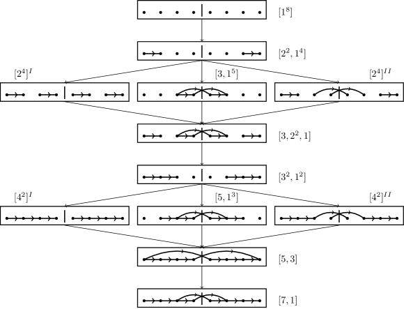
Figure 13: Hasse diagram of $SO(8)$ nilpotent deformations going from top (UV) to bottom (IR) where all simple roots are present and every corresponding simple string is connecting adjacent $A$-branes or in the case of the last simple root, two $A$-branes are connected to the $BC$-mirror.

Finally, much like what we have seen in $SU(N)$, most flows include the simple addition of a root/string and therefore are obvious. However, there are a few cases that are not so immediately clear. We work them out here in the case of $SO(8)$ and note that the methods below extend to the higher rank $SO$ groups.

• $[2^{2},1^{4}]\rightarrow[3,1^{5}]$: We can add to $\alpha_{1}$ the highest positive root $\alpha_{2,1,3,2,4}=\alpha_{1}+2\alpha_{2}+\alpha_{3}+\alpha_{4}$ (identified with the matrix $E_{1,7}+E_{2,8}$). This setup is represented by the matrix $E_{1,2}+E_{7,8}+\epsilon\left(E_{1,7}+E_{2,8}\right)$, which belongs to the same orbit as $E_{3,4}+E_{5,6}+E_{3,5}+E_{4,6}$ and corresponds to the diagram involving the set of simple strings $\{\alpha_{3},\alpha_{4}\}$.

• $[3,2^{2},1]\rightarrow[3^{2},1^{2}]$: We can add the non-simple string $\alpha_{2}+\alpha_{3}+\alpha_{4}$ to the initial set $\{\alpha_{1},\alpha_{3},\alpha_{4}\}$. This gives the matrix $E_{1,2}+E_{7,8}+E_{3,4}+E_{5,6}+E_{3,5}+E_{4,6}+\epsilon\left(E_{2,6}+E_{3,7}\right)$ which is similar to the matrix $E_{1,2}+E_{7,8}+E_{2,3}+E_{6,7}$.

• $[3^{2},1^{2}]\rightarrow[5,1^{3}]$: We can add the non-simple string $\alpha_{2}+\alpha_{3}+\alpha_{4}$ to the set of simple roots $\{\alpha_{1},\alpha_{2}\}$ to obtain the matrix $E_{1,2}+E_{7,8}+E_{2,3}+E_{6,7}+\epsilon\left(E_{2,6}+E_{3,7}\right)$. This matrix is similar to the one corresponding to the set of strings $\{\alpha_{2},\alpha_{3},\alpha_{4}\}$.

• $[5,1^{3}],[4^{2}]^{II}\rightarrow[5,3]$ Starting from the set of simple roots $\{\alpha_{2},\alpha_{3},\alpha_{4}\}$ of $[5,1^{3}]$ we can add the positive root $\alpha_{1}+\alpha_{2}+\alpha_{3}$ to obtain the equivalent set $\{\alpha_{1},\alpha_{2},\alpha_{3},\alpha_{2}+\alpha_{3}+\alpha_{4}\}$.

  Similarly, starting from the set of simple roots $\{\alpha_{1},\alpha_{2},\alpha_{4}\}$ of $[4^{2}]^{II}$ we can add the positive non-simple root $\{\alpha_{2},\alpha_{3},\alpha_{4}\}$ again to obtain the same Weyl equivalent set $\{\alpha_{1},\alpha_{2},\alpha_{3},\alpha_{2}+\alpha_{3}+\alpha_{4}\}$.

3.3 $Sp(N)$

Recall that in F-theory, we realize the $Sp(N)$-type gauge theories by a non-split $I_{N}$ fiber. In terms of 7-branes, this involves the transverse intersection of a stack of D7-branes with an $O7^{-}$-plane along a common 6D subspace. In the IIA realization of this algebra, we can also consider a stack of D6-branes on top of an $O6^{+}$-plane.

For our present purposes, we can merge the $A$-branes pairwise on each side of the mirror. This then yields $N$ nodes on each side of the mirror but with the particularity that a two-pronged string can stretch from a single composite node, as seen in table 1. Zooming out, the two-pronged string – which corresponds to the long simple root of $Sp(N)$ – gets squished into a double arrow coming out of the same node and connecting to its mirror-image across the $BC$-branes. This means that, unlike with $SO(2N)$ algebras, we can now draw a double string stretching from the same node and crossing the $BC$-mirror. The simple root $\alpha_{N}$ of figure 14 is one example of the $N$ double string connections that can be stretched that way. In terms of the IIA description, the change in orientation of the mirror means we can now draw all of the same string junctions as for $SO(2N)$, but we also have an additional $2N$ possible roots which correspond to double connections coming out of the same node (something that was not allowed in $SO(2N)$). The set of simple roots/strings for $Sp(N)$ is given in figure 14.

Figure 14: Brane diagram of strings/roots stretching, for $Sp(N)$. The orientifold is once again represented by a mirror (vertical line). The strings corresponding to simple roots are illustrated by arrows stretching between the branes and reflected across the mirror. We note that the longer root $\alpha_{N}$ corresponds to the two-pronged string being squeezed into a single double arrow crossing the mirror, ensuring that the charge differences are still respected.

The set of simple strings (as illustrated in figure 14) along with the reflecting mirror ensures that odd parts in the partition of $2N$ must appear with even multiplicity. This exactly matches the constraint that, in the partitions used to parametrize the nilpotent orbits of $Sp(N)$, the multiplicity of odd parts must be even. Furthermore, $Sp(N)$ also contains distinguished orbits, which involve the presence of one or more non-simple root.

Following the same conventions as before, we use the following matrices as the nilpositive part of the basis for $\mathfrak{sp}_{N}$:

• $N(N-1)/2$ one-pronged strings $E_{\mathrm{1-pronged}}=E_{i,j}-(-1)^{j-i}E_{2N-j+1,2N-i+1}$ with $1\leq i<j\leq N$ corresponding to one-pronged strings stretching from the $i^{th}$ to the $j^{th}$ $A$-brane as well as their reflections. That is the strings stretching between the $(2N-j+1)^{th}$ and the $(2N-i+1)^{th}$ nodes which are on the right-hand side of the mirror. These correspond to the $\mathfrak{su}_{N}\subset\mathfrak{sp}_{N}$ nilpositive generators.

• $N(N-1)/2$ two-pronged strings $E_{\mathrm{2-pronged}}=E_{i,2N-j+1}+(-1)^{j-i}E_{j,2N-i+1}$ with $1\leq i<j\leq N$ corresponding to two-pronged strings stretching between the $i^{th}$ and $(2N-j+1)^{th}$ nodes as well as the $j^{th}$ and $(2N-i+1)^{th}$ nodes.

• $N$ double strings $X_{\mathrm{doubled}}=2E_{i,2N-i+1}$ with $1\leq i\leq N-1$ and the long simple string $X_{N}=E_{N,N+1}$. These correspond to double-pronged strings merged together into single double connections. They stretched from the $i^{th}$ to the $(2N-i+1)^{th}$ node.

The $N$ doubled strings coming out of the same node are the only new roots which were not present in $\mathfrak{so}_{2N}$.

We give the Hasse diagram of nilpotent orbits for $Sp(3)$ in figure 15 to illustrate the possible string junctions. Flows between each level in the Hasse diagrams follow the same rules as for the $SO$ groups.

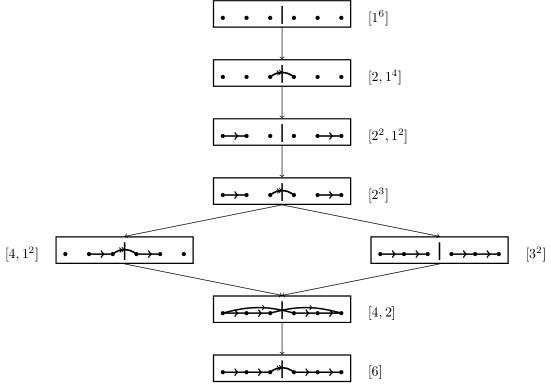
Figure 15: Hasse diagram of $Sp(3)$ nilpotent deformations going from top (UV) to bottom (IR) where all simple roots are turned on and every corresponding simple strings are connecting the $A$-branes. In the case of the last simple root, a double connection stretches from the last node and connects across the mirror, ensuring charge conservation.

3.4 An Almost Classical Algebra: $G_{2}$

We next consider the exceptional Lie group $G_{2}$. Even though the Lie algebra of $G_{2}$ is technically an exceptional Lie group, the fact that it can easily be embedded inside the Lie algebra of $SO(7)$ makes it behave almost identically. Furthermore, as we are going to encounter this algebra even when dealing only with classical quivers it is useful to have a closer look at exactly how one might want to describe it.

First, we note that the monodromy of $G_{2}$ is the same as for $SO(7)$ and $SO(8)$ that is, there are a total of four $A$-branes and a $B$ with a $C$ brane. Thus, we can start from the $SO(7)$ configuration which has four $A$-branes with one stuck on the $BC$-mirror (see figure 12). Then, we note that for $G_{2}$, the roots $\alpha_{1}$ and $\alpha_{3}$ are identified while $\alpha_{2}$ is left untouched. Namely, the branching $SO(7)\rightarrow G_{2}$ takes $\alpha_{1}+\alpha_{3}\rightarrow\alpha_{1}$ and $\alpha_{2}\rightarrow\alpha_{2}$. Therefore, we obtain the positive roots listed in figure 16.

Figure 16: Brane diagram of strings/roots stretching, for $G_{2}$. The $B$ and $C$-branes are turned into an orientifold denoted by a mirror (vertical line) and one of the $A$-branes is squeezed onto it. Furthermore, the first $A$-brane is “linked” to the middle one (as if it were also merged onto the mirror), so that the first and third root of $SO(7)$ join together as the first root of $G_{2}$ (as dictated by the quotient which takes $SO(7)\rightarrow G_{2}$). The strings corresponding to simple roots are illustrated by arrows stretching between the branes and reflected across the mirror.

The matrix representation is taken directly from $SO(7)$. For the positive simple roots we have:

$$X_{1} \equiv E_{1,2}+E_{6,7}+\sqrt{2}\left(E_{3,4}+E_{4,5}\right),$$ (3.20)

$$X_{2} \equiv E_{2,3}+E_{5,6}.$$ (3.21)

The other four positive roots are given by:

$$\left[X_{1},X_{2}\right] =E_{1,3}-E_{5,7}-\sqrt{2}\left(E_{2,4}-E_{4,6}\right),$$ (3.22)

$$\left[\left[X_{1},X_{2}\right],X_{1}\right] =2\sqrt{2}\left(E_{1,4}+E_{4,7}\right)-2\left(E_{2,5}+E_{3,6}\right),$$ (3.23)

$$\left[\left[\left[X_{1},X_{2}\right],X_{1}\right],X_{1}\right] =6\left(E_{1,5}-E_{3,7}\right),$$ (3.24)

$$\left[\left[\left[\left[X_{1},X_{2}\right],X_{1}\right],X_{1}\right],X_{2}\right] =6\left(E_{1,6}+E_{2,7}\right).$$ (3.25)

As a result, we can now give the four non-trivial nilpotent orbits of $G_{2}$ in terms of strings (see figure 17). We note that, once again, we have a simple correspondence with partitions of $7$, illustrated by the groupings allowed from the associated string junctions. The ordering is a total ordering rather than a mere partial ordering (unlike for most larger groups), and the flows from one orbit to the other follow from the fact that they are projections of the previously studied $SO(7)$ symmetry.

Figure 17: Hasse diagram of $G_{2}$ nilpotent deformations going from top (UV) to bottom (IR) where both simple roots are present so that both corresponding simple strings are there to connect all $7$-branes and mirror image branes

3.5 Nilpotent Orbits for Exceptional Algebras

We now turn our attention to the exceptional Lie algebras $E_{6,7,8}$. These distinguish themselves from the classical algebras in several ways. First, their nilpotent orbits are not simply described by partitions but rather by Bala-Carter labels. These labels are in one-to-one correspondence with a weighted Dynkin diagram and a set of roots. Interestingly, when the matrix representations of these roots are added together, their Jordan block decomposition still yields a unique partition. Thus, we can still parametrize the nilpotent orbits of $E_{6,7,8}$ by partitions of $27$, $56$, and $248$ (corresponding to the dimension of their respective fundamental representations). These partitions arise from the branching of the fundamental of $E_{N}$ to the $SU(2)$ associated to the nilpotent orbit. However, there does not exist a simple set of rules or restriction on these partitions like we have seen for the classical Lie algebras. Thus this classification is very limited.

By making use of string junctions and the brane configuration describing these algebras, it is however possible to gain a little more insight into the structure of nilpotent orbits for these exceptional groups. Physically, we know that the $E_{N}$ symmetries are given by $A^{N-1}BC^{2}$ or equivalently $A^{N}XC$ brane configurations. The advantage of using the description with an $X$-brane is that we can now branch $E_{N}$ to $SU(N)\times U(1)$, where the $SU(N)$ piece is represented by $N$ $A$-branes and $N-1$ ordinary open strings (i.e. one beginning and one end) stretching between them. States charged under the $U(1)$ factor necessarily involve multi-prong strings which attach to this stack of $A$-branes and also involve the $XC$ stack. This procedure matches identically the initial setup used for describing $SO(2N)$ symmetries. The only difference is that we now have a generalized mirror made out of an $X$ and a $C$ brane instead of simply a $B$ and $C$ branes. This means that it now takes a three-pronged string stretching from three $A$-branes to attach to the $XC$-mirror in order to conserve the charges. Indeed, the charges from an $X$ and a $C$ brane now sum to $[3,0]$ which is exactly three times that of an $A$ brane. As a result we obtain the brane and string configurations given in figure 18.

Figure 18: Brane diagram of strings/roots stretching between the $A$, $X$, and $C$-branes making up the $E_{6,7,8}$ symmetry (see [59]). The $A$-branes are denoted by black circles, the $X$-brane by an empty triangle and the $C$-brane by an empty square. The dashed lines represent the position of branch cuts. Again, these branch cuts are not drawn in subsequent pictures. To the right we give the corresponding Dynkin diagram with simple roots numbered.

We then treat the $X$ and $C$ branes together as a generalized mirror and use the short-hand picture of figure 19 where the $XC$-mirror is represented by an $\times$ inside a circle to differentiate it from the vertical line that represented the $BC$-mirror for the orientifold seen in the $SO(N)$ symmetries.

Figure 19: Brane diagram of strings/roots stretching, for $E_{6,7,8}$. The $X$ and $C$-branes are turned into a generalized mirror denoted by a crossed circle. The strings corresponding to simple roots are illustrated by arrows stretching between the branes. We note that the distinguished root $\alpha_{2}$ corresponds to the three-pronged string and indeed is made of three-legs attaching to the $XC$-mirror in order to respect the difference in charges between the $A$, $X$, and $C$ branes.

This $XC$-mirror is more complicated than the simply reflecting mirror for the classical algebras. Indeed, we can think of this mirror as fragmenting the partitions of $27$, $56$, and $248$ according to their branching rules. The fundamental representation of $E_{N}$ branches to irreducible representations of $SU(N)\times U(1)$ as:

$$\mathbf{27}\rightarrow\mathbf{\overline{15}}_{0}+\mathbf{6}_{1}+\mathbf{6}_{\scalebox{0.75}[1.0]{-}1}, \text{for }E_{6}\rightarrow SU(6)\times U(1),$$ (3.26)

$$\mathbf{56}\rightarrow\mathbf{\overline{21}}_{\scalebox{0.75}[1.0]{-}2}+\mathbf{21}_{2}+\mathbf{\overline{7}}_{6}+\mathbf{7}_{\scalebox{0.75}[1.0]{-}6}, \text{for }E_{7}\rightarrow SU(7)\times U(1),$$ (3.27)

$$\mathbf{248}\rightarrow\mathbf{63}_{0}+\mathbf{56}_{3}+\mathbf{\overline{56}}_{\scalebox{0.75}[1.0]{-}3}+\mathbf{28}_{\scalebox{0.75}[1.0]{-}6}+\mathbf{\overline{28}}_{6}+\mathbf{\overline{8}}_{\scalebox{0.75}[1.0]{-}9}+\mathbf{8}_{9}+\mathbf{1}_{0}, \text{for }E_{8}\rightarrow SU(8)\times U(1).$$ (3.28)

Here, $\mathbf{15}$ is the two-index anti-symmetric representation of $SU(6)$ and $\mathbf{21}$ is the two-index anti-symmetric representation of $SU(7)$. For the $E_{8}$ case, $\mathbf{63}$ is the adjoint, $\mathbf{28}$ is the two-index anti-symmetric, $\mathbf{56}$ is the three-index anti-symmetric and $\mathbf{8}$ is the fundamental representation of $SU(8)$. For the adjoint representations of $E_{6}$ and $E_{7}$ we also have:

$$\mathbf{78}\rightarrow+\mathbf{35}_{0}+\mathbf{20}_{1}+\mathbf{20}_{\scalebox{0.75}[1.0]{-}1}+\mathbf{1}_{2}+\mathbf{1}_{\scalebox{0.75}[1.0]{-}2}+\mathbf{1}_{0}, \text{for }E_{6}\rightarrow SU(6)\times U(1),$$ (3.29)

$$\mathbf{133}\rightarrow\mathbf{45}_{0}+\mathbf{35}_{\scalebox{0.75}[1.0]{-}4}+\mathbf{\overline{35}}_{4}+\mathbf{7}_{8}+\mathbf{\overline{7}}_{\scalebox{0.75}[1.0]{-}8}+\mathbf{1}_{0}, \text{for }E_{7}\rightarrow SU(7)\times U(1).$$ (3.30)

By embedding $SU(N)$ inside $E_{N}$ in this manner, we see that positive strings can be described by any set of one-pronged strings between the $N$ $A$-branes or any three-pronged string attaching to three $A$-branes and stretching to the $XC$-mirror. Furthermore, $E_{6}$ also allows a six-pronged string attaching all of its $A$-branes to the $XC$-mirror, as illustrated by the trivial representation $\mathbf{1}_{2}$ in its branching. This string corresponds to the highest root of $E_{6}$. $E_{7}$ also allows six-pronged strings, as seen by the presence of $\mathbf{\overline{7}}_{\scalebox{0.75}[1.0]{-}8}$ in its branching (this is indeed the six index anti-symmetric representation of $SU(7)$). Finally, $E_{8}$ not only allows six-pronged strings (as seen by the six index anti-symmetric $\mathbf{\overline{28}}_{6}$ representation), but it also allows for eight different nine-pronged strings, which connect all eight $A$-branes to the $XC$-mirror with a double connection stretching from one of the eight $A$-branes. These rules follow directly from the structure of the exceptional algebras, as shown in [49, 59]. To illustrate these situations, we depict the highest roots of $E_{6}$, $E_{7}$ and $E_{8}$ in figures 20, 21, and 22.

Figure 20: Highest roots of $E_{6}$ represented by its corresponding six-pronged string. It stretches from all six $A$-branes and attaches to the $X$ and $C$ branes represented by the crossed circle.

Figure 21: Highest roots of $E_{7}$ represented by its corresponding six-pronged string. It stretches from the six left-most $A$-branes and attaches to the $X$ and $C$ branes represented by the crossed circle.

Figure 22: Highest roots of $E_{8}$ represented by its corresponding nine-pronged string. It stretches from all eight $A$-branes (attaching twice onto the first one) to the $X$ and $C$ branes represented by the crossed circle.

In order to describe each nilpotent orbit, we now need to rely more heavily on the matrix representation. As a result, we associate to each simple string of figure 18 a matrix in the fundamental representation of $E_{N}$. Any choice of basis will yield the same results, but for reference we give the simple roots in Appendix D and use the method of [60] to obtain the remaining non-simple roots.

Next, we proceed just as with the classical algebras. Namely, we start with $N$ $A$-branes next to an $XC$-mirror and start attaching more and more small string deformations until we reach the deepest nilpotent orbit. To every string junction diagram we associate a matrix representation which belongs to some nilpotent orbit. We can differentiate between nilpotent orbits based on the Bala-Carter label or the partition associated to the matrix (by Jordan block decomposition). For instance, the diagram involving the first two simple roots of $E_{6}$ is represented by the matrix $X_{1}+X_{3}$ where

$$X_{1} =E_{1,2}+E_{12,13}+E_{15,16}+E_{17,18}+E_{19,20}+E_{21,22},$$

$$X_{3} =E_{2,3}+E_{10,12}+E_{11,15}+E_{14,17}+E_{20,23}+E_{22,24}.$$

This matrix $X_{1}+X_{3}$ has Jordan block decomposition $[3^{6},1^{9}]$ and is associated to the Bala-Carter label $A_{2}$.

Much as in the case of the classical algebras, multiple diagrams belong to the same equivalence class. Thus, in order to keep our diagrams as simple as possible, we choose representative string junction diagrams that only make use of the simple strings from figure 18 whenever possible. Indeed, once again we identify some distinguished orbits as those which cannot be described solely by a set of simple roots and necessarily involve non-simple roots. Furthermore, while any string junction yielding the proper partition is valid, for simplicity we select configurations with the minimum number of strings required (with as few non-simple strings as possible) so that the addition of only a single positive root $\epsilon\cdot X_{k}$ is required to flow to the nearest nilpotent orbit. We illustrate the nilpotent orbits of $E_{6}$, $E_{7}$, and $E_{8}$ in figures 23, 24, 25. The Hasse diagrams labeled by just their Bala-Carter labels can be found in e.g. the Appendix of [61], which summarizes several aspects regarding nilpotent orbits of exceptional algebras.

We see that we can move from one nilpotent orbit to the next by small deformations, just like we did for the classical groups. Furthermore, we can describe every orbit using only simple strings except for the distinguished ones. These distinguished orbits once again require the presence of one (or two, for $E_{8}(a_{7})$) non-simple roots.

3.5.1 The Non-Simply Laced $F_{4}\subset E_{6}$

Finally, we note that $F_{4}\subset E_{6}$ is obtained from $E_{6}$ by a very simple identification of simple roots:

$$\alpha_{2}^{E_{6}} =\alpha_{1}^{F_{4}},$$

$$\alpha_{4}^{E_{6}} =\alpha_{2}^{F_{4}},$$

$$\alpha_{3}^{E_{6}}+\alpha_{5}^{E_{6}} =\alpha_{3}^{F_{4}},$$

$$\alpha_{1}^{E_{6}}+\alpha_{6}^{E_{6}} =\alpha_{4}^{F_{4}},$$ (3.31)

where $\alpha_{1}^{F_{4}}$ and $\alpha_{2}^{F_{4}}$ denote the first two short roots of $F_{4}$ while $\alpha_{3}^{F_{4}}$ and $\alpha_{4}^{F_{4}}$ denote the longer ones. As a result, we can also simply give the Hasse diagram of $F_{4}$ as a subset of the one from $E_{6}$.

Figure 23: Hasse diagram of $E_{6}$ nilpotent deformations going from top (UV) to bottom (IR) where all simple roots are present, and every corresponding simple string connects adjacent $A$-branes, or in the case of the second simple root, three $A$-branes are connected to the $XC$-mirror. For ease of exposition we only list the set of strings rather than the complete string junction diagrams for each case.

Figure 24: Hasse diagram of $E_{7}$ nilpotent deformations going from top (UV) to bottom (IR) where all simple roots are present, and every corresponding simple string connects adjacent $A$-branes, or in the case of the second simple root, three $A$-branes connect to the $XC$-mirror.

Figure 25: Hasse diagram of $E_{8}$ nilpotent deformations going from top (UV) to bottom (IR) where all simple roots are present, and every corresponding simple string connects adjacent $A$-branes, or in the case of the second simple root, three $A$-branes connect to the $XC$-mirror.

4 Higgsing and Brane Recombination

In the previous section, we showed how to generate the entire nilpotent cone of a semi-simple algebra using the combinatorics of string junctions. In particular, the operation of “adding a string” reproduces the expected partial ordering based on orbit inclusion. We now use this analysis to study Higgs branch flows for 6D SCFTs. Our main task here will be to study the effects of brane recombination triggered by vevs for 6D conformal matter.

We first remark that the picture in terms of string junctions leads to a simple description of Higgsing with semi-simple deformations. Recall that a semi-simple element is one that is diagonalizable (in particular, not nilpotent). Since all the quiver-like gauge theories consist of stacks of $A^{N}$ branes with either a $BC$ or $XC$ plane, we may join an open string from one stack of $A$-branes to the next, continuing from left to right across the entire quiver. This leads to a “peeling off” of the corresponding $7$-brane, and has the effect of reducing the rank of each of the gauge algebras by one in both the classical case and the exceptional case.

Much more subtle is the case of T-brane deformations. For the most part, we confine our analysis to the case of quiver-like theories in which all the gauge groups are classical (see figures 26, 27, 28, 29). Even in these cases, the matter content of the partial tensor branch can still be strongly coupled, as evidenced by $SO-SO$ 6D conformal matter. Nonetheless, we will still be able to develop systematic sets of rules to extract the IR fixed point obtained from a given T-brane deformation in such cases.

To some extent, the necessary data is encoded by judiciously applying Hanany-Witten moves involving suspended D6-branes. Such moves were used in [62], for instance, to extract different presentations of a given 6D SCFT. To apply the Hanany-Witten analysis of that work to the case at hand, we will need to extend it in two respects. First of all, to cover the case of quiver-like theories with $SO$ gauge algebras, such brane maneuvers sometimes result in a formally negative number of D6-branes [22, 37]. Additionally, in the case of short quivers, the data specified by pairs of nilpotent orbits will produce correlated effects in the resulting IR fixed points. To address both points, we will need to extend the available results in the literature.

As we have already mentioned, our main focus will be on tracking brane recombinations as triggered by the condensation of open strings. In the context of 6D SCFTs, all of this occurs in a small localized region of the base of the non-compact elliptic threefold. Macroscopic data such as the surviving flavor symmetries corresponds to the asymptotic behavior of non-compact $7$-branes that pass through this singular region, but which also extend out to the boundary of the non-compact base. This also means that, provided we hold fixed the total asymptotic $7$-brane charge present in the configuration, we can consider any number of “microscopic processes” which could appear in the physics of brane recombination.

One such process which we shall often use is the creation of brane / anti-brane pairs localized in the region near the 6D SCFT. We denote such an anti-brane by $\overline{A}$ and use it in annihilation processes such as:

$$A+\overline{A}\rightarrow\text{no branes.}$$ (4.1)

Strictly speaking, such a physical process would generate radiation. The only sense in which we are really using these objects is to count the overall Ramond Ramond charge asymptotically far away from the configuration. In this sense, there will be little distinction between an anti-brane and a “negative / ghost-brane.” Since we are primarily interested in determining the end outcome of Higgsing, we use these $\overline{A}$-branes as a combinatorial tool which must disappear at the final stages of our analysis through processes such as line (4.1). We refer to this as having a “Dirac sea” of $A/\overline{A}$ pairs of $7$-branes.

Much as in the case of a general configuration of plus and minus charges in electrodynamics, a lowest energy configuration is obtained by allowing charges to freely move through a material. In much the same way, we shall allow the branes and anti-branes to redistribute. Our main physical condition is that the net $7$-brane charge is unchanged by such processes, and also, that no anti-brane charge remains uncanceled in any final configuration obtained after Higgsing.

We also remark that from the standpoint of renormalization group flow, these sorts of microscopic details are expected to be irrelevant at long distances. Said differently, while there could, a priori, be different UV completions in the full framework of quantum gravity, such details will not matter in determining possible fixed points obtained after a Higgs branch deformation. The brane maneuvers indicated here are of this sort and are used as a tool to analyze possible fixed points.

Including these formal structures is useful in that it allows us to make sense of the resulting 6D SCFT, even when the ranks of the intermediate gauge groups are negative numbers of small magnitude. This procedure has been used in [22, 37, 63, 30, 40] as a way to track the effects of Higgs branch flows in certain 6D SCFTs. We will return to this point in section 5.

Our main focus in this section will be on determining the Higgs branch flows associated with the classical algebras, since in these cases there is also a gauge theory description available for some Higgs branch flows in terms of vevs of conventional hypermultiplets. Any nilpotent orbit is then described by stretching the appropriate strings as described in section 3. We then need to propagate the deformation by removing some strings as we move deeper into the quiver, which allows us to read off the resulting gauge symmetries that are left over in the IR. We explain these propagation rules in the following section.

Figure 26: Tensor branch of the UV quiver-like theory with just $SU(N)$ gauge algebras.

Figure 27: Tensor branch of the UV quiver-like theory with just $SO(2N)$ gauge algebras. The full tensor branch also includes additional $Sp(N-4)$ gauge algebras coming from blowing up the conformal matter between D-type collisions.

Figure 28: Tensor branch of the UV theory with just $SO(2N-1)$ gauge algebras. The full tensor branch also includes additional $Sp$ gauge algebras coming from blowing up the conformal matter between D-type collisions. Any deformation with partition $\mu=[\{\mu_{i}\}]$ in $SO(2N-1)$ is equivalent to the partition $\nu=[\{\mu_{i}\},3]$ in $SO(2N+2)$.

Figure 29: UV theory for $Sp(N)$.

Before that, however, we need to introduce the possibility of anti-branes. Indeed, while the nodes in the $SU(N)$ quivers all have the same number of branes on each level (namely $N$ $A$-branes), the other classical algebras do not. For instance, a quiver with $SO(2N)$ flavor in the UV will alternate between $N$ and $N-4$ $A$-branes on the $\mathfrak{so}_{2N}$ and $\mathfrak{sp}_{N}$ levels respectively. This introduces an additional complication in that we may end up with configurations that have more strings stretching between branes (as dictated by the nilpotent orbit configuration of section 3) than are available according to the gauge group on the quiver node. We remedy this situation by extracting as many extra $A$ branes as necessary out of the brane / anti-brane “Dirac sea” to draw the proper number of string junctions. These extra branes are then immediately canceled with the same number of anti-branes.

For example, the theory with $SO(8)$ flavor symmetry has gauge symmetries alternating between $\mathfrak{sp}_{0}$ (i.e. a trivial gauge group associated with an “unpaired tensor” [64]) and $\mathfrak{so}_{8}$, and the nilpotent orbit $[4^{2}]^{I}$ uses strings stretching between every brane (i.e. all four $A$-branes and their images have at least one string attached). However, $\mathfrak{sp}_{0}$ only has the $BC$-mirror and no $A$-brane. So, in order to describe the $[4^{2}]^{I}$ nilpotent orbit, we must introduce four $A$-branes through which we can stretch strings (on each side of the mirror) and then add them with four anti-branes. This also applies to the non-simply laced classical algebras, since they can be obtained from Higgs branch flows of $SO($even$)$ quiver-like theories [5].

Notably, there are a few cases, even for SO- and Sp-type quivers, which require non-perturbative ingredients such as E-string / small instanton deformations. In these cases, the number of tensor multiplets in the 6D SCFT also decreases. Our method using brane / anti-brane pairs carries over to these situations and allows us to obtain a complete picture of Higgs branch flows in these cases as well. We use this feature in section 5 to determine IR fixed points in the case of short quivers.

Our plan in the rest of this section is as follows: first, we discuss a IIA realization of quiver-like theories with classical gauge groups, and especially the treatment of Hanany-Witten moves in such setups. After this, we state our rules for how a T-brane propagates into the interior of a quiver with classical gauge algebras. We then illustrate with several examples the general procedure for Higgsing such theories. This provides a uniform account of brane recombination and also agrees in all cases with the result expected from related F-theory methods (when available). We also comment on some of the subtleties associated with extending this to the case of quiver-like theories with exceptional algebras.

4.1 IIA Realizations of Quivers with Classical Gauge Groups

To aid in our investigation of Higgs branch flows for 6D SCFTs, it will also prove convenient to use the type IIA realizations of the quiver-like theories with classical algebras, as used previously in references [65, 66, 67, 62]. In the case of quivers with $SU$ gauge group factors, each classical gauge group factor is obtained from a collection of D6-branes suspended between spacetime filling NS5-branes, with non-compact “flavor” D8-branes emanating “out to infinity.” The case of $SO$ algebras on the partial tensor branch is obtained by also including $O6^{-}$-planes coincident with each stack of D6-branes. In this case, the NS5-branes can fractionate to $\frac{1}{2}$ NS5-branes. Working in terms of these fractional branes, there is an alternating sequence of $O6^{+}$ and $O6^{-}$ planes, and correspondingly an alternating sequence of $SO$ and $Sp$ gauge group factors. This all matches up with the F-theory realization of these theories, where each $SO$ factor originates from an $I_{n}^{\ast}$ fiber and each $Sp$ factor from a non-split $I_{m}$ fiber.

The utility of this suspended brane description is that we can write several equivalent brane configurations which realize the same IR fixed point via “Hanany-Witten moves,” much as in the original reference [68] and its application to 6D SCFTs in reference [62]. This provides a convenient way to uniformly organize the data of Higgs branch deformations generated by nilpotent orbits. In fact, we will shortly demonstrate that using these brane moves along with some additional data (such as the appearance of brane / anti-brane pairs) provides an intuitive method for determining the resulting fixed points in both long and short quivers.

Since we will be making heavy use of the IIA realization in our analysis of Higgs branch flows, we now discuss such constructions in greater detail. In our analysis, we will also consider formal versions of Hanany-Witten moves which would seem to involve a negative number of branes. These cases are closely connected with strong coupling phenomena (such as the appearance of small instanton transitions and spinor representations) and can be fully justified in the corresponding F-theory realization of the same SCFT. Indeed, the description in terms of Hanany-Witten moves extends to the F-theory description, so we will interchangeably use the two conventions when the context is clear.

4.1.1 SU($N$)

We begin with a quiver-like theory with $L-1$ tensor multiplets and for each one a paired $SU(N)$ gauge group factor. The UV theory has a tensor branch given by the quiver

,

which is realized in terms of the IIA brane setup:

.

From the point of view of the D6-branes, the D8-branes specify boundary conditions, which are controlled by the Nahm equations [69]. These pick three ($X^{i}$, $i=1,2,3$) out of the $N^{2}-1$ scalars controlling the Higgs branch and relates them to the distance $t$ of the intersection point by

$$X^{i}\sim\frac{T^{i}}{t}.$$ (4.2)

The generators $T^{i}$ describe an $SU(2)$ subgroup of the flavor symmetry SU($N$), whose embedding is captured by a partition of $N$. This happens on both sides of the quiver. Thus all the data we need in order to study Higgs branch flows of the UV theory are two partitions $\mu_{L}$ and $\mu_{R}$ of $N$ and the length $L$.

A partition $\mu$ of $N$ is given in terms of $l\leq N$ integers $\mu^{i}$ with $\mu^{1}\geq\mu^{2}\geq\dots\geq\mu^{l}$ and $\mu^{1}+\mu^{2}+\dots\mu^{l}=N$. In the corresponding brane realization, the two partitions describe the separation of the stack of $N$ D8-branes on each side into smaller stacks

.

The brane picture is particularly useful because we can easily read off the IR theory from it. This works by applying Hanany-Witten moves, which swap a D8-brane and an NS5-brane, until all of the D8-branes are balanced. Looking at the stack of $\mu_{L}^{1}$ D8-branes left of the first NS5-branes, we can measure its imbalance by the difference $\Delta n$ of D6-branes departing from the right and arriving on the left. A balanced stack would have $\Delta n=0$, but for the setup depicted above we find $\Delta n=\mu_{L}^{1}$ instead. After performing the Hanany-Witten move described in figure 30, $\Delta n$ becomes

$$\Delta n^{\prime}=\Delta n-1\qquad\text{with}\qquad\Delta=n_{2}-n_{1}\quad\text{and}\quad\Delta^{\prime}=n_{3}-n_{2}^{\prime}\,.$$ (4.3)

Hence, we have to perform exactly $\Delta n=\mu_{L}^{1}$ Hanany-Witten moves to balance this stack.

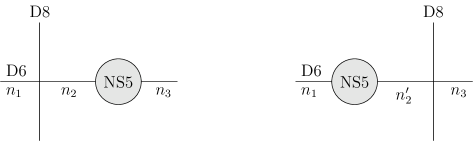
Figure 30: The basic operation of swapping a D8- and NS5-branes. The relation between the number of D6-branes stretching between the D8-brane and the NS5-brane before ($n_{2}$) and after ($n_{2}^{\prime}$) the swapping is given by $n_{2}^{\prime}=n_{1}+n_{3}-n_{2}+1$.

One can always balance all D8-branes provided that the length of the quiver $L$ is large enough. This constraint will become important when we discuss short quivers in section 5. Once all D8-branes are balanced, the resulting IR quiver gauge theory can be read off by using the building blocks

.

Applying subsequent Hanany-Witten moves results in a simple, algebraic description of the Higgs branch flows. Let us, for simplicity, consider very long quivers. In this case it is sufficient to just focus on one partition, i.e. $\mu_{L}$, since the analysis on the right-hand side is perfectly analogous. Using the fact that a stack of $\mu^{i}_{L}$ D8-branes moves $\mu^{i}_{L}$ NS5-branes to the right until it is balanced, we can read off the flavor symmetries of the IR theory directly from the partition. However, obtaining the number of D6-branes stretched between each pair of adjacent NS5s is slightly more complicated. If we denote this number as $n_{i}$ between the $i$’s and $i+1$’s NS5s we find the following recursion relation

$$(n_{i})_{j}=\begin{cases}(n_{i})_{j-1}-\mu_{L}^{j}+i&\text{for }i<\mu_{L}^{j}\\ (n_{i})_{j-1}&\text{otherwise}\,.\end{cases}$$ (4.4)

Here $(n_{i})_{j}$ denotes the $n_{i}$ after the $j$’th stack of NS5-branes has been balanced. Hence, the initial condition is $(n_{i})_{0}=N$, and we are interested in $(n_{i})_{l_{L}}$, which describes the number of D6-branes once all D8-branes have been balanced. An example for $N=6$ is $\mu=[3\,2\,1]$, for which we find

$$(n_{i})_{1} =\begin{pmatrix}4&5&6&6&\dots\end{pmatrix}$$ (4.5)

$$(n_{i})_{2} =\begin{pmatrix}3&5&6&6&\dots\end{pmatrix}$$

$$(n_{i})_{3} =\begin{pmatrix}3&5&6&6&\dots\end{pmatrix}$$

with the resulting IR quiver

.

4.2 SO($2N$), SO($2N+1$) and Sp($N$)

Gauge groups SO($2N$), SO($2N+1$) and Sp($N$) arise if the setup from the last subsection is extended to include O6 orientifold planes placed on top of the D6-branes. In particular, assume we have $N$ physical D6-branes. Each of these has a mirror image under the $\mathbb{Z}_{2}$ orientifold action $\Omega$, and thus we have in total $2N$ 1/2 D6-branes. Their Chan-Paton factors transform under $\Omega$ as $\Omega\lambda=M\lambda^{T}M^{-1}$. Since $\Omega^{2}=1$, we therefore find two different solutions for $M$, which are denoted as $M_{\pm}=\pm M_{\pm}^{T}$. Each of these solutions gives rise to a distinguished orientifold action $\Omega_{\pm}$. Only massless open string excitations satisfying $\Omega_{\pm}\lambda=-\lambda^{T}$ survive the orientifold projection. Depending on whether $\Omega_{-}$ (O6^-) or $\Omega_{+}$ (O6⁺) is used, the resulting gauge group is either SO($2N$) or Sp($N$). If a single 1/2 D6-branes is exactly on top of the O6^- plane, it becomes its own mirror and we obtain the gauge group SO($2N+1$). Similar to the D6-branes, a single NS5-branes on the orientifold plane splits into two half NS5-branes:

Here, we depict a stack of 1/2 D6-branes on O6^- with a solid line and a stack of 1/2 D6-branes on O6⁺ with a dashed line. Because the D6-charge of the O6⁺ differs by 4 from the one of the O6^- the number of 1/2 D6-branes changes from $n$ to $n+n\,\mathrm{mod}\,2-8$ and back.

SO($2N-1$)
SO($2N$)
Sp($N$)

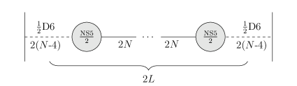
Figure 31: Suspended brane realization of UV quivers with SO($2N$-1), SO($2N$), and Sp($N$) flavor symmetries.

There are three different classes UV SCFTs which we can now realize in terms of suspended branes depicted in figure 31. To study their Higgs branch flow, we follow the same approach as in the SU($N$) case: first, we choose two partitions, which each describe an embedding of $\mathfrak{su}_{2}$ into the corresponding flavor symmetry algebra. These control how the stacks of 1/2 D8-branes on the left and right side of the quiver are split into smaller stacks. Finally, we apply Hanany-Witten moves to these stack until they are balanced.

It is convenient to combine the D6-brane charge of the orientifold planes with the contribution from the 1/2 D6-branes. In this case, rules for the Hanany-Witten shown in figure 30 still apply and we can use the results from the last subsection. The only thing we have to keep in mind is that we are now counting 1/2 D6-branes.

4.3 Propagation Rules

In this section, we present a set of rules for working out Higgs branch deformations in the case of quivers with classical gauge algebras. The main idea is to consider each stack of $7$-branes wrapped over a curve and strings that stretch from one stack to the next. To visualize the possible locations where such strings can begin and end, we will use the same diagrammatic analysis developed in section 3 to track these breaking patterns. When such a string is present, it signals the presence of a brane recombination move, and the corresponding brane becomes non-dynamical (having become attached to a non-compact $7$-brane on the boundary of the quiver). On each layer, we introduce a directed graph, as dictated by a choice of nilpotent orbit. This tells us how to connect the branes into “blobs” after recombination. We want to see how these blobs recombine, both with the non-compact branes at the end of quiver and the compact branes further in the interior.

On each consecutive level of the quiver (i.e. for each gauge algebra in the quiver), we draw the same string configuration with a few modifications according to the following rules for propagating Higgs branch flows into the interior of a quiver:

• First, we consider blobs made only of $A$-branes. That is, only one-pronged strings are involved and there is no crossing or touching the mirror. These configurations cover all possible orbits of $SU(N)$. In such cases, the one-pronged strings get removed one at a time (per blob) so that one $A$-brane is added back (to each blob) at each step. These steps can be visualized in the example of $SU(6)$ nilpotent orbits given in figure 32.

• Next, we consider cases with a two-pronged string, but in which both legs are disjoint (unlike $\alpha_{N}$ for $Sp(N)$) so that no loop is formed. In this case, the propagation follows the same rule as for one-pronged strings. Indeed in such configurations each leg becomes independent and they individually behave like one-pronged strings. This is the case for $SO(2N)$ whenever the two-pronged string $\alpha_{N}$ is present but not the string $\alpha_{N-1}$ below it. (See for instance the partition $[2^{4}]^{II}$ for $SO(8)$ in figure 33).

• Now suppose (without loss of generality) that branes $A_{1},A_{2},\cdots,A_{n}$ are connected via simple one-pronged strings and a two-pronged string attaches the $i^{th}$ and $n^{th}$ brane to the mirror ($1\leq i<n$). Then, for the next $n-i$ levels, the right-most leg moves one step to the left (attaching to the brane $A_{n-1},A_{n-2},\cdots,A_{n-i}$) and the right-most one-pronged string below it is removed, namely $\alpha_{n}$ followed by $\alpha_{n-1},\cdots,\alpha_{n-i}$. After these $n-i$ steps, both legs overlap and the right-most leg cannot move any further. Instead, we then move the second leg one step to the left so that one leg stretches from $\alpha_{n-i-1}$ and the other stretches from $\alpha_{n-i}$. We can now repeat the previous steps once by moving the right-most leg one brane to the left (and removing $\alpha_{n-i-1}$) so that it overlaps with the left-most leg. This process ends whenever the two-pronged string with both legs overlapping is the last one of the group and it is then simply removed for the next node in the quiver. (See for instance the partitions $[5,3]$ or $[7,1]$ for $SO(8)$ in figure 33).

• Finally we can have groups of $K$ branes involving the short root $\alpha_{N-1}$ of $SO(2N-1)$, which connects the $N^{th}$ $A$-brane to the one merged onto the mirror. In this case, the first step consists of lifting the short string above the middle brane so that it becomes a doubled-arrow string crossing the mirror and connecting $K-1$ branes. The next steps in the propagation are then identical to the ones described in the previous point. (See for instance the partitions $[7,1^{2}]$ or $[9]$ for $SO(9)$ in figure 37).

We note that in terms of partitions, these steps simply translate into every part being reduced by $1$, so that the partition $[\mu_{1},\mu_{2},\cdots,\mu_{i},1^{k}]$ goes to $[\mu_{1}-1,\mu_{2}-1,\cdots,\mu_{i}-1,1^{k+i}]$ after each step until there are no more parts with $\mu_{i}>1$, and we are left with the trivial partition (corresponding to the total absence of strings).

4.4 Higgsing and Brane Recombination

Once we have propagated the strings according to the above rules, we are ready to read off the residual gauge symmetry on each node. To do so, we note that the strings force connected branes on each side of the mirror to coalesce so that a blob of $K$ $A$-branes behaves like a single $A$-brane. We can then directly read off the gauge symmetry that is described by the resulting collapsed brane configuration.

For $SU(N)$ quivers, which do not involve a mirror, strings group $A$-branes without any ambiguity, as no $B$ or $C$ brane is present. Thus, the residual gauge symmetry is given by the number of groups formed at each level. For instance, if only one simple string stretches between two $A$-branes, these branes coalesce, and we are left with $N-1$ separate groups of strings on this level. This yields the residual gauge symmetry $\mathfrak{su}_{N-1}$ as illustrated in the first orbit of $SU(6)$ (see figure 32).

Similarly, a blob with $K$ branes connected by strings on each side of a mirror turns an $\mathfrak{so}_{2N}$ algebra into $\mathfrak{so}_{2(N-K+1)}$, $\mathfrak{so}_{2N-1}$ into $\mathfrak{so}_{2(N-K+1)-1}$, and $\mathfrak{sp}_{N}$ into $\mathfrak{sp}_{N-K+1}$. The same is true if the blob consists of branes on both sides of the mirror connected by double-pronged strings. However, if the blob consists of branes connected by a double-arrowed string, then the blob of connected branes gets merged onto the mirror. As a result, an $\mathfrak{so}_{2K}$ algebra will turn into $\mathfrak{so}_{2K-1}$, and $\mathfrak{so}_{2K-1}$ into $\mathfrak{so}_{2K-2}$. (See for instance the [7,1] diagrams at the bottom of figure 33.) We note that the propagation rules listed above prevent such a configuration from ever appearing on a level with $\mathfrak{sp}_{N}$ gauge symmetry.

In some cases, the $\mathfrak{so}$ quivers require the introduction of “anti-branes.” In our figures, we denote a brane by a filled in circle (black dot) and an anti-brane by an open circle. At the final step, all such anti-branes must disappear by pairing up with other coalesced branes, deleting such blobs from the resulting configuration. This further reduces the number of leftover blobs which generate the residual gauge symmetry.

Note that there are also situations where the number of anti-branes is larger than the number of available blobs of branes on a given layer. This occurs whenever the number of D6-branes in the type IIA suspended brane realization formally becomes negative, signaling that the perturbative type IIA description has broken down, and F-theory is required to construct the theory in question. Nevertheless, it is still useful to write down a “formal IIA quiver,” which includes negative numbers of D6-branes and hence negative gauge group ranks. Additionally, as we will now show with examples, our picture of brane / anti-brane nucleation can be adapted to these situations if we allow extra anti-branes at a given layer to move to other layers and annihilate other blobs of branes.

Consider, for instance, the partition $[5,3]$ of $SO(8)$ requires the presence of four $A$-branes on the first quiver node, which only has $\mathfrak{sp}_{0}$ symmetry. Thus, we also need to introduce four anti-branes to compensate. Only one blob of branes is formed on each side of the mirror, so only one of the four anti-branes is used to cancel it, and we are left with three anti-branes. The first anti-brane is used to collapse the $-1$ curve it is on. The second anti-brane is distributed to the next $\mathfrak{so}$ quiver node and the third anti-brane is distributed to the next $\mathfrak{sp}$ quiver node, where it is used to either reduce the gauge symmetry from $\mathfrak{sp}_{K}$ to $\mathfrak{sp}_{K-1}$ or, if $K=0$, to blow down this next $-1$ curve. The anti-brane that lands on a quiver node with an $\mathfrak{so}$ algebra also reduces the residual symmetry according to the following rules:

$$\mathfrak{so}_{N} \overset{\overline{A}}{\rightarrow}\mathfrak{so}_{N-1}\text{ for }N\geq 8,$$

$$\mathfrak{so}_{7} \overset{\overline{A}}{\rightarrow}\mathfrak{g}_{2},$$

$$\mathfrak{g}_{2} \overset{\overline{A}}{\rightarrow}\mathfrak{su}_{3},$$

$$\mathfrak{so}_{6}\simeq\mathfrak{su}_{4} \overset{\overline{A}}{\rightarrow}\mathfrak{su}_{3},$$

$$\mathfrak{su}_{3} \overset{\overline{A}}{\rightarrow}\mathfrak{su}_{2},$$

$$\mathfrak{so}_{5}\simeq\mathfrak{sp}_{2} \overset{\overline{A}}{\rightarrow}\mathfrak{sp}_{1}\simeq\mathfrak{su}_{2},$$

$$\mathfrak{so}_{4} \overset{\overline{A}}{\rightarrow}\mathfrak{so}_{3}\simeq\mathfrak{su}_{2},$$

$$\mathfrak{so}_{3}\simeq\mathfrak{su}_{2} \overset{\overline{A}}{\rightarrow}\mathfrak{su}_{1}\simeq\emptyset.$$ (4.6)

Note that for classical quiver theories, there can never be more than four anti-branes, since the quiver nodes with $\mathfrak{sp}$ gauge symmetry only have four fewer branes than their neighboring $\mathfrak{so}$ nodes.

We illustrate all of these steps through the examples of $SU(6)$, $SO(8)$, $SO(10)$, $SO(9)$, and $Sp(3)$ in figures 32, 33, 35, 37, and 38 respectively. Explicit examples of $\mathfrak{g}_{2}\overset{\overline{A}}{\rightarrow}\mathfrak{su}_{3}$ and $\mathfrak{su}_{3}\overset{\overline{A}}{\rightarrow}\mathfrak{su}_{2}$ can only be found when dealing with “short quivers,” which we discuss in section 5.

	UV           string junction           IR
$[1^{6}]$		$[1^{6}]$
	$\vdots$

$[2,1^{4}]$		$[2,1^{4}]$
	$\vdots$

$[2^{2},1^{2}]$		$[2^{2},1^{2}]$
	$\vdots$

$[2^{3}]$$,1$								$[3,1^{3}]$
	$\vdots$						$\vdots$

$[3,2,1]$		$[3,2,1]$
	$\vdots$

$[3^{2}]$$,1$								$[4,1^{2}]$
	$\vdots$						$\vdots$

$[4,2]$		$[4,2]$
	$\vdots$

$[5,1]$		$[5,1]$
	$\vdots$

$[6]$		$[6]$
	$\vdots$

Figure 32: Nilpotent deformations of the $SU(6)$ quiver from the UV configuration of figure 26. Each subfigure corresponds to the quiver diagram of a nilpotent orbit with strings propagating through. The quivers have been rotated to go from top to bottom (rather than left to right) to fit on the page. On the left-hand side of each subfigure we have the setting in the UV with each $-2$ curve containing an $\mathfrak{su}_{6}$ gauge algebra, while on the right-hand side we give the IR theory induced by the strings stretched in the middle diagram. The theories are ordered from top to bottom according to their partial ordering of RG flows, which matches their mathematical ordering. The corresponding partitions are given on the side.

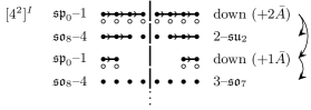
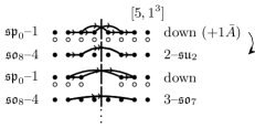
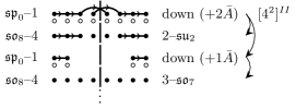
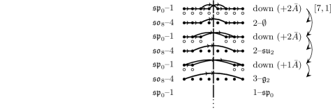
Figure 33: Nilpotent deformations of the $SO(8)$ quiver from the UV configuration of figure 27. Each subfigure corresponds to the quiver diagram of a nilpotent obit with strings propagating into the interior of the quiver. The quivers have been rotated to go from top to bottom (rather than left to right) to fit on the page. On the left-hand side of each subfigure, we have the initial UV theory with alternating $-1$ and $-4$ curves containing $\mathfrak{sp}_{0}$ and $\mathfrak{so}_{8}$ respectively. On the right-hand side, we give the IR theory induced by the strings stretched in the middle diagram. The vertical line denotes the $BC$-mirror. Whenever anti-branes are required, they are denoted by white circle below their $A$-brane counterparts. In some cases, there are extra anti-branes indicated in parentheses on the right (which occur when there are more groups of $A$-branes than anti-branes). The first one is used to blow-down the $-1$ curve it is on (indicated by the word “down”), while the others get distributed on the following quiver nodes as indicated by the side arrows on the right. The theories are ordered from top to bottom according to their partial ordering of RG flows. The corresponding partitions are given on the side.

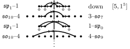
Figure 34: Nilpotent deformations of the $SO(10)$ quiver from the UV configuration of figure 27. See figure 33 for additional details on the notation and conventions.

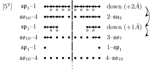
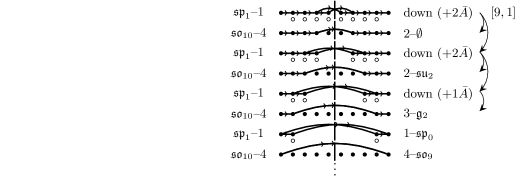
Figure 35: (continued) Nilpotent deformations of the $SO(10)$ quiver from the UV configuration of figure 27. See figure 33 for additional details on the notation and conventions.

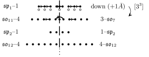
Figure 36: Nilpotent deformations of the $SO(9)$ quiver from the UV configuration of figure 28. See figure 33 for additional details on the notation and conventions.

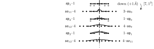
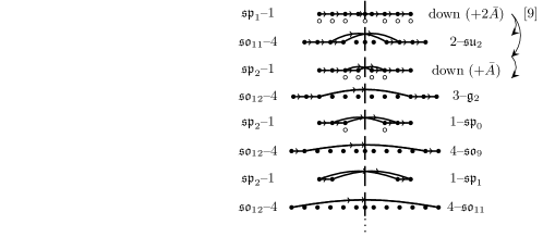
Figure 37: (continued) Nilpotent deformations of the $SO(9)$ quiver from the UV configuration of figure 28. See figure 33 for additional details on the notation and conventions.

Figure 38: Nilpotent deformations of the $Sp(3)$ quiver from the UV configuration of figure 29. See figure 33 for additional details on the notation and conventions.

4.5 Comments on Quiver-like Theories with Exceptional Algebras

It is natural to ask whether the propagation rules given for quivers with classical algebras also extend to theories with exceptional algebras. In principle, we expect this to follow from our description of the nilpotent cone in terms of multi-pronged string junctions. Indeed, we have already explained that at least for semi-simple deformations, there is no material distinction between the quivers of classical and exceptional type.

That being said, we expect our analysis of nilpotent deformations to be more subtle in this case. Part of the issue is that even in the case of the D-type algebras, to really describe the physics of brane recombination, we had to go onto the full tensor branch so that both $SO$ and $Sp$ gauge algebras could be manipulated (via brane recombination). From this perspective, we need to understand brane recombination in 6D conformal matter for the following configurations of $(E_{N},E_{N})$ conformal matter:

$$[E_{6}],1,3,1,[E_{6}]$$ (4.7)

$$[E_{7}],1,2,3,2,1,[E_{7}]$$ (4.8)

$$[E_{8}],1,2,2,3,1,5,1,3,2,2,1,[E_{8}].$$ (4.9)

Said differently, a breaking pattern which connects two E-type algebras will necessarily involve a number of tensor multiplets. For the most part, one can work out a set of “phenomenological” rules which cover nearly all cases involving quivers with $E_{6}$ gauge algebras, but its generalization to $E_{7}$ and $E_{8}$ appears to involve some new ingredients beyond the ones introduced already in this paper. For all these reasons, we defer a full analysis of these cases to future work.

5 Short Quivers

In the previous section, we demonstrated that the physics of brane recombination accurately recovers the expected Higgs branch flows for 6D SCFTs. It is reassuring to see that these methods reproduce – but also extend – the structure of Higgs branch flows obtained through other methods. The main picture we have elaborated on is the propagation of T-brane data into the interior of a quiver-like gauge theory.

The main assumption made in these earlier sections is the presence of a sufficient number of gauge group factors in the interior of the quiver so that this propagation is independent of other T-brane data associated with other flavor symmetry factors. In this section we relax this assumption by considering “short quivers” in which the number of gauge group factors is too low to prevent such an overlap. There has been very little analysis in the 6D SCFT literature on this class of RG flows.

Using the brane recombination picture developed in the previous section, we show how to determine the corresponding 6D SCFTs generated by such deformations. We mainly focus on quivers with classical algebras, since this is the case we presently understand most clearly. Even here, there is a rather rich structure of possible RG flows.

There are two crucial combinatorial aspects to our analysis. First of all, we use open strings to collect recombined branes into “blobs.” Additionally, to determine the scope of possible deformations, we introduce brane / anti-brane pairs, as prescribed by the rules of section 4. To track the effects of having a short quiver, we gradually reduce the number of gauge group factors until the brane moves on either side of the quiver become correlated. As a result, we sometimes reach configurations in which the anti-branes cannot be eliminated. We take this to mean that we have not actually satisfied the D-term constraints in the quiver-like gauge theory.

The procedure we outline also has some overlap with the formal proposal of reference [37] (see also [63]), which analyzed Higgs branch flows by analytically continuing the rank of gauge groups to negative values. Using our description in terms of anti-branes, we show that in many cases, the theory we obtain has an anomaly polynomial which matches to these proposed theories. We also find, however, that in short quivers (which were not analyzed in [37]) this analytic continuation method sometimes does not produce a sensible IR fixed point. This illustrates the utility of the methods developed in this paper.

In the case of sufficiently long quiver-like theories, there is a natural partial ordering set by the nilpotent orbits in the two flavor symmetry algebras. In the case of shorter quivers, the partial ordering becomes more complicated because there is (by definition) some overlap in the symmetry breaking patterns on the two sides of a quiver. In many cases, different pairs of nilpotent orbit wind up generating the same IR fixed point simply because most or all of the gauge symmetry in the quiver has already been Higgsed. We show in explicit examples how to obtain the corresponding partially ordered set of theories labeled by pairs of overlapping nilpotent orbits. We refer to these as “double Hasse diagrams” since they merge two Hasse diagrams of a given flavor symmetry algebra.

To illustrate the main points of this analysis, we primarily focus on illustrative examples in which the number of gauge group factors in the interior of a quiver is sufficiently small and / or in which the size of the nilpotent orbits is sufficiently large so that there is non-trivial overlap between the breaking patterns on the left and right. For this reason, we often work with low rank gauge algebras such as $\mathfrak{su}(4)$ and $\mathfrak{so}(8)$ and a small number of interior gauge group factors, though we stress that our analysis works in the same way for all short quivers.

The rest of this section is organized as follows. First, we show how to obtain short quivers as a limiting case in which we gradually reduce the number of gauge group factors in a long quiver. We then turn to a study of nilpotent hierarchies in these models, and we conclude this section with a brief discussion of the residual global symmetries after Higgsing in a short quiver.

5.1 From Long to Short Quivers

In this subsection, we determine how T-brane data propagating from the two sides of a quiver becomes intertwined as we decrease the number of gauge groups / tensor multiplets. It is helpful to split up this analysis according to the choice of gauge group appearing, so we present examples for each different choices of gauge algebras.

5.1.1 $SU(N)$ Short Quivers

We begin with quiver-like theories with $\mathfrak{su}$ gauge algebras. Applying the Hanany-Witten rules from section 4.1 to the type IIA realization of the $SU(N)$ theories, we have that:

$$k_{\textrm{NS5}}\geq\textrm{Max}\{\mu_{L}^{1},\mu_{R}^{1}\}+1$$ (5.1)

for left and right partitions $\mu_{L}=[\mu^{i}]$, $\mu_{R}=[\mu^{j}]$ respectively. Here, $k_{\textrm{NS5}}$ denotes the number of NS5-branes in the corresponding type IIA picture. When this condition is violated, it is impossible to balance the D8-branes. Note that $k_{\textrm{NS5}}$ is also equal to one plus the number of $-2$ curves $N_{-2}=N_{T}$ the number of tensor multiplets in the UV quiver, so we may equivalently write this condition as

$$\mathrm{Max}\{\mu_{L}^{1},\mu_{R}^{1}\}\leq N_{-2},$$ (5.2)

where $N_{-2}$ denotes the number of $-2$ curves in the UV quiver. This is equivalent to saying that, when only one nilpotent deformation (either $\mu_{L}$ or $\mu_{R}$) is implemented over the UV quiver (either the left or right partition), there has to be at least one $-2$ curve whose fiber remains untouched by the deformation.

Assuming this restriction is obeyed, we can straightforwardly produce any short $SU(N)$ quiver given a UV quiver and a pair of nilpotent orbits. Before giving the general formula, however, let us look at a concrete example: consider a UV theory of $SU(5)$ over five $-2$ curves, and apply the nilpotent deformations of $[3,2]$ – $[2^{2},1]$, where no interaction between the orbits take place. This theory can be written as:

$$[3,2]:\,\,\overset{\mathfrak{su}(2)}{2}\,\,\underset{[N_{f}=1]}{\overset{\mathfrak{su}(4)}{2}}\,\,\underset{[N_{f}=1]}{\overset{\mathfrak{su}(5)}{2}}\,\,\underset{[SU(2)]}{\overset{\mathfrak{su}(5)}{2}}\,\,\underset{[N_{f}=1]}{\overset{\mathfrak{su}(3)}{2}}\,\,:[2^{2},1]$$ (5.3)

where the notation $[N_{f}=1]$ refers to having one additional flavor on each corresponding gauge algebra.

We now decrease the length of the quiver and gradually turn it into a short quiver. We decrease the number of $-2$ curves one at a time, and when the nilpotent deformation from the left and right overlaps, we simply add the rank reduction effect together linearly. After each step we get:

$$[3,2]:\,\,\overset{\mathfrak{su}(2)}{2}\,\,\underset{[N_{f}=1]}{\overset{\mathfrak{su}(4)}{2}}\,\,\underset{[SU(3)]}{\overset{\mathfrak{su}(5)}{2}}\,\,\underset{[N_{f}=1]}{\overset{\mathfrak{su}(3)}{2}}\,\,:[2^{2},1]$$ (5.4)

$$[3,2]:\,\,\overset{\mathfrak{su}(2)}{2}\,\,\underset{[SU(3)]}{\overset{\mathfrak{su}(4)}{2}}\,\,\underset{[SU(2)]}{\overset{\mathfrak{su}(3)}{2}}\,\,:[2^{2},1]$$ (5.5)

At this stage we are unable to decrease the length of the quiver any further without violating the constraint of (5.2).

We note that each step changes the global symmetry, the gauge symmetry, or both. In particular, after the second step we no longer see a node with the UV gauge group $SU(5)$. The global symmetries also change at each step, which will be discussed further in 5.4.

Let us consider another example of a short quiver with $SU(N)$ gauge groups. If we take the UV quiver theory to be:

$$[SU(6)]\,\,\overset{\mathfrak{su}(6)}{2}\,\,\overset{\mathfrak{su}(6)}{2}\,\,\overset{\mathfrak{su}(6)}{2}\,\,\overset{\mathfrak{su}(6)}{2}\,\,\overset{\mathfrak{su}(6)}{2}\,\,[SU(6)]$$ (5.6)

and apply the following pair of nilpotent deformations denoted by partitions $\mu_{L,R}$:

$$\mu_{L}=[5,1],\ \ \mu_{R}=[2^{3}]$$ (5.7)

we obtain the resulting IR theory:

$$\underset{[N_{f}=1]}{\overset{\mathfrak{su}(2)}{2}}\,\,\overset{\mathfrak{su}(3)}{2}\,\,\overset{\mathfrak{su}(4)}{2}\,\,\underset{[SU(3)]}{\overset{\mathfrak{su}(5)}{2}}\,\,\underset{[N_{f}=1]}{\overset{\mathfrak{su}(3)}{2}}\,.$$ (5.8)

We illustrate another example with $SU(5)$ UV gauge group and partitions $\mu_{L}=[5]$, $\mu_{R}=[4,1]$ in figure 39, making the brane recombination explicit.

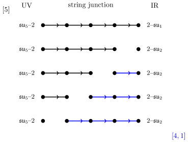
Figure 39: An $SU(N)$ short quiver brane picture, the pair of nilpotent deformation being $\mu_{L}=[5]$, $\mu_{R}=[4,1]$ on $SU(5)$ UV theory and four $-2$ curves. The figure is arranged so that the left deformation starts from the top and propagates downwards (in black) while the right deformation starts on the bottom and propagates upwards (blue).

In general, let us define the conjugate partitions of the left and right nilpotent orbits to be $\rho_{L}:=\mu_{L}^{T}$ and $\rho_{R}:=\mu_{R}^{T}$ and denote their number of elements as $N_{L}^{\prime}$ and $N_{R}^{\prime}$, with the index counting from each of their starting point, respectively. Then, the gauge group rank at the $m^{\text{th}}$ node is given by

$$r_{m}=N-\sum_{i=m+1}^{N_{L}^{\prime}}\rho_{i}^{L}-\sum_{j=(N_{-2})-m+1}^{N_{R}^{\prime}}\rho_{j}^{R},$$ (5.9)

with the UV gauge group equal to $SU(N)$.

5.1.2 Interlude: $SO$ and $Sp$ Short Quivers

In the case of quivers with $SU$ gauge groups, the Higgsing of the corresponding quiver-like gauge theories is controlled by vevs for weakly coupled hypermultiplets. In this case, the physics of brane recombination primarily serves to simplify the combinatorics associated with correlated breaking patterns in the quiver. Now, an important feature of the other quiver-like theories with flavor groups $SO$ or $Sp$ is the more general class of possible Higgs branch flows as generated by 6D conformal matter. Recall that on the full tensor branch of such a theory, we have a gauge group consisting of alternating classical gauge groups. These gauge groups typically have bifundamental matter (in half-hypermultiplets of $SO\times Sp$ representations), which in turn leads to Higgs flows generated by “classical matter,” much as in the case of the $SU$ quivers. There are, however, more general Higgs branch flows connected with vevs for conformal matter. Recall that these are associated with a smoothing deformation for a collapsed $-1$ curve, namely the analog of a small instanton transition as in the case of the E-string theory. The combinatorics associated with this class of Higgs branch flows is more subtle, but as we have already remarked, the brane / anti-brane description correctly computes the resulting IR fixed points in this case as well.

By definition, in the case of a short quiver, the effects of Higgsing on the two sides of the quiver become correlated. It is therefore helpful to distinguish a few specific cases of interest as the size of the nilpotent orbit / breaking pattern continues to grow. As the size of the nilpotent orbit grows, the appearance of a small instanton deformation becomes inevitable. The distinguishing feature is the extent to which small instanton transitions become necessary to realize the corresponding Higgs branch flow. When there is at least one $-1$ curve remaining in the tensor branch description of the Higgsed theory, we refer to this as a case where the nilpotent orbits are “touching.” The end result is that so many small instanton deformations are generated that the tensor branch of the resulting IR theory has no $-1$ curves at all. We refer to this as a “kissing case” since the partitions are now more closely overlapping. Increasing the size of a nilpotent orbit beyond a kissing case leads to a problematic configuration: There are no more small instanton transitions available (as the $-1$ curves have all been used up). We refer to these as “crumpled cases.” In terms of our brane / anti-brane analysis, this leads to configurations with $\overline{A}$ branes which cannot be canceled off. Such crumpled configurations are inconsistent, and must be discarded. Summarizing, we refer to the different sorts of overlapping nilpotent orbit configurations as:

• A “touching” configuration is one in which all gauge groups of the quiver-like theory are at least partially broken, but at least one $-1$ curve remains in the tensor branch of the Higgsed theory.

• A “kissing” configuration is defined as one in which all groups of the quiver-like theory are at least partially broken, and there are no $-1$ curves remaining in the Higgsed theory.

• A “crumpled” configuration is defined as one in which the orbits have become so large that there are left over $\overline{A}$ branes which cannot be canceled off, and therefore such configurations are to be discarded.

Of course, there are also nilpotent orbits which are uncorrelated, as will occur whenever the quiver is sufficiently long or the nilpotent orbits are sufficiently small, which we can view as “independent cases.” Such “independent / touching cases” fall within the scope of the long quiver analysis that we have discussed previously – the latter just marginally so. We illustrate all four configurations in figure 40 for $SO(10)$ with partitions $\mu_{L}=\mu_{R}=[9,1]$ going from an “independent” (long) quiver configuration all the way down to a forbidden “crumpled” configuration.

Following the IIA realization from section 4.1, we can formally perform Hanany-Witten moves even when small instanton transitions occur by allowing for a negative number of D6-branes, or in the string-junction picture by allowing brane / anti-brane pairs as intermediate steps in our analysis. The formula (5.2) generalizes to the other quiver-like theories with classical algebras:

$$k_{\frac{1}{2}\textrm{NS5}}\geq\textrm{Max}\{\mu_{L}^{1},\mu_{R}^{1}\}+1,\text{ rounded up to the nearest even number.}$$ (5.10)

$$\iff N_{T}\geq\textrm{Max}\{\mu_{L}^{1},\mu_{R}^{1}\}.$$ (5.11)

Here $k_{\frac{1}{2}\textrm{NS5}}$ is the number of half NS5-branes in the corresponding type IIA picture, and equals one plus the number of tensor multiplets in the UV quiver ($N_{T}=2N_{-4}+1$) in the UV. One might worry that this becomes meaningless whenever small instanton transitions occur. Indeed, the quivers described after such transitions all have matter with spinor representations and therefore no perturbative type IIA representation. While we can formally draw suspended brane diagrams with gauge groups of negative ranks, physically there is no corresponding suspended brane diagram. However, by analytically continuing the anomaly polynomials of these quivers to the case of negative ranks, we find perfect agreement with the anomaly polynomials of the actual, physical theory constructed via F-theory. This gives us strong reason to believe that the rules for Hanany-Witten moves should likewise carry over to the formal IIA brane diagrams, which implies that the formal quiver must be of length at least $\textrm{Max}\{\mu_{L}^{1},\mu_{R}^{1}\}$.

Finally, from the brane / anti-brane analysis, we note that there should not be any residual $\overline{A}$’s in the IR theories. Any configuration yielding extra $\overline{A}$’s that cannot be canceled are said to “crumple” and are therefore forbidden. This further restricts the above constraints from Hanany-Witten moves.

As an example, an $SO(2N)$ quivers with partitions

$$\mu_{L}=\mu_{R}=[2N-1,1]$$ (5.12)

requires that

$$k_{\frac{1}{2}\textrm{NS5}}\geq 2N+4,$$ (5.13)

which is a strictly stronger lower bound than the one imposed by equation 5.11. This particular example is illustrated for $SO(10)$ with partitions $\mu_{L}=\mu_{R}=[9,1]$ in the “crumpling” example of subfigure 40(d).

5.1.3 $SO(2N)$ Short Quivers

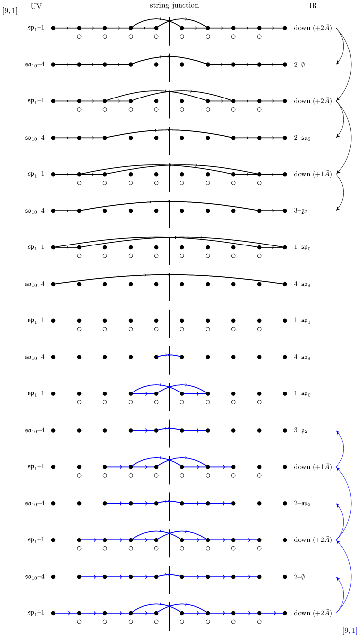
(a) Independent example: Partitions $\mu_{L}=\mu_{R}=[9,1]$ on $17$ curves.

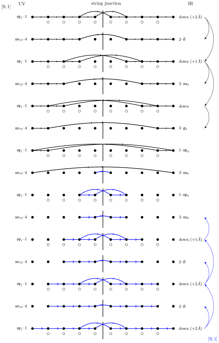
(b) Touching example: Partitions $\mu_{L}=\mu_{R}=[9,1]$ on $15$ curves. Some but not all $-1$ curves participate in small instanton deformations.

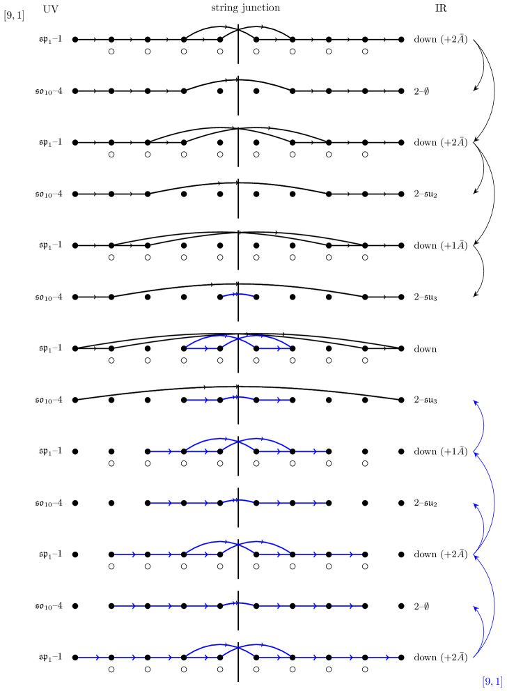
(c) Kissing configuration: Partitions $\mu_{L}=\mu_{R}=[9,1]$ on $13$ curves. Every $-1$ curve participates in a small instanton / smoothing deformation.

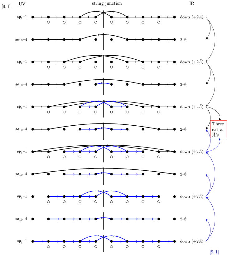
(d) Crumpled configuration: Partitions $\mu_{L}=\mu_{R}=[9,1]$ on only $11$ curves. Too many $\overline{A}$’s are generated.

Figure 40: Holding fixed the partitions $\mu_{L}=\mu_{R}=[9,1]$ we can decrease the number of curves to go from a long quiver (where the deformations are independent) all the way to a forbidden crumpled configuration.

As we did in the $SU(N)$ case, we now show how to produce short $SO(2N)$ quivers beginning from long ones. For our first example, we consider the following formal $SO(8)$ quiver:

$$[5,3]:\,\,\overset{\mathfrak{sp}(-3)}{1}\,\,\overset{\mathfrak{so}(4)}{4}\,\,\overset{\mathfrak{sp}(-1)}{1}\,\,\overset{\mathfrak{so}(7)}{4}\,\,1\,\,\overset{\mathfrak{so}(8)}{4}\,\,\overset{\mathfrak{sp}(-1)}{1}\,\,\overset{\mathfrak{so}(4)}{4}\,\,\overset{\mathfrak{sp}(-3)}{1}\,\,:[4^{2}],$$ (5.14)

which is converted into the following F-theory quiver:

$$[5,3]:\,\,\overset{\mathfrak{su}(2)}{2}\,\,\overset{\mathfrak{g}_{2}}{3}\,\,1\,\,\underset{[SU(2)]}{\overset{\mathfrak{so}(7)}{3}}\,\,{\overset{\mathfrak{su}(2)}{2}}\,\,[4^{2}].$$ (5.15)

If we reduce the length by one, we would get a kissing theory (that is, every $-1$ curve has been blown-down):

$$[5,3]:\,\,\underset{[N_{f}=1]}{\overset{\mathfrak{su}(2)}{2}}\,\,\underset{[SU(2)]}{\overset{\mathfrak{su}(3)}{2}}\,\,\underset{[N_{f}=1]}{\overset{\mathfrak{su}(2)}{2}}\,\,[4^{2}]\,.$$ (5.16)

However, if we try to further reduce the length, we will reach a case that “crumples” due to an excess of $\overline{A}$’s that cannot be canceled, and therefore is invalid.

We can also keep the length of the quiver fixed and follow the RG flows along the nilpotent orbits (we will discuss this part in more detail in section 5.3). Consider the same example, but now increase the right nilpotent orbit from $[4^{2}]$ to $[5,3]$. We still get an “independent” theory:

$$[5,3]:\,\,\overset{\mathfrak{su}(2)}{2}\,\,\overset{\mathfrak{g}_{2}}{3}\,\,\underset{[SU(2)]}{1}\,\,\overset{\mathfrak{g}_{2}}{3}\,\,\overset{\mathfrak{su}(2)}{2}\,\,[5,3]\,.$$ (5.17)

If we further increase the right nilpotent orbit to $[7,1]$, we will instead get a kissing theory:

$$[5,3]:[SU(2)\times SU(2)]\,\,{\overset{\mathfrak{su}(2)}{2}}\,\,\overset{\mathfrak{su}(2)}{2}\,\,\underset{[N_{f}=3/2]}{\overset{\mathfrak{su}(2)}{2}}\,\,2\,\,[7,1]\,.$$ (5.18)

At this step, increasing the left orbit also up to $[7,1]$ would give a crumpled configuration, which is not allowed.

We can describe all of this in general using the string junction picture previously developed. Following our previous proposal for long quiver brane pictures, we start from the outermost curves of the quiver, where we initialize our nilpotent deformation in terms of the string junction picture. Then, following the $SO/Sp$ propagation rule, we propagate the clusters from both sides towards the middle simultaneously. In the case of short quivers, strings from both sides might end up touching, sharing different intermediate layers, in which case the gauge group reduction effects from both sides add together. For example, figure 41 illustrates the action of $\mu_{L}=[9,1]$, $\mu_{R}=[5^{2}]$ for $SO(10)$ in a theory with $11$ curves.

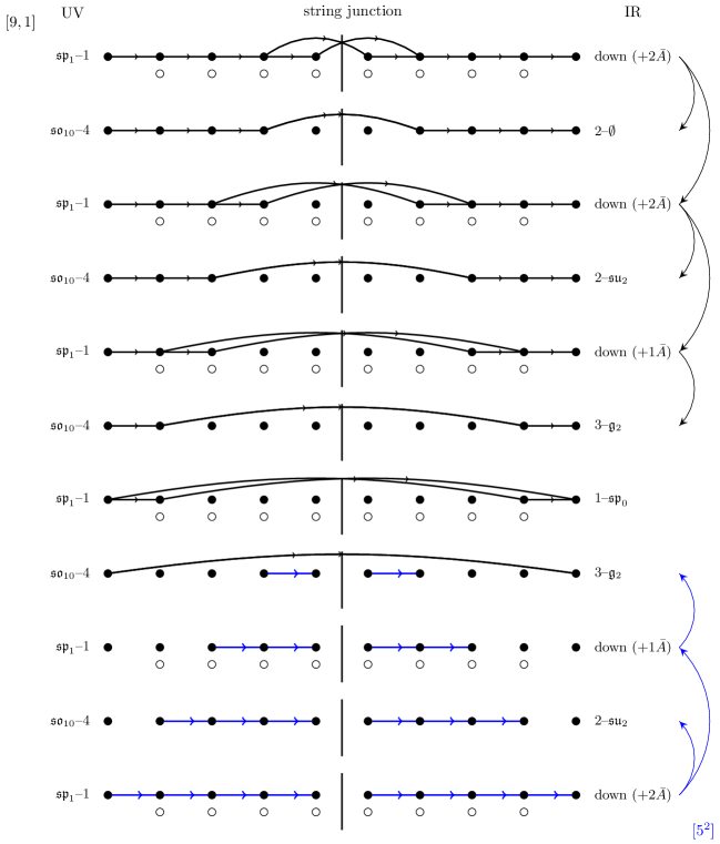
Figure 41: An $SO(10)$ short quiver brane picture for nilpotent deformations $\mu_{L}=[9,1]$, $\mu_{R}=[5^{2}]$. Additional branes are needed in order to construct the associated string diagrams, which in turn introduces anti-branes (depicted by white circles). The figure is arranged so that the left deformation starts from the top and propagates downwards (in black) while the right deformation starts on the bottom and propagates upwards (in blue). After the blowdown and Higgsing procedures, all but one of the $-1$ curves are blown down, and the remaining curves now have self-intersection $-2$ or $-3$.

We note that we can have new situations that could not previously occur in long quivers. The first novelty comes from the fact that levels with $\mathfrak{so}$ gauge algebra can now be Higgsed by two $\overline{A}$’s: one from the left nilpotent deformation and one from the right. As a result, we get configurations where two anti-branes accumulate on the same $-4$ curve and reduce it to a $-2$ curve. The resulting gauge algebra is then given by two applications of the rules for anti-brane reductions given in section 4.4. Figure 42 illustrates this phenomenon for a pair of theories, which respectively involve the reductions:

$$\mathfrak{so}_{7}\overset{\overline{A}}{\rightarrow}\mathfrak{g}_{2}\overset{\overline{A}}{\rightarrow}\mathfrak{su}_{3}$$ (5.19)

$$\mathfrak{so}_{6}\simeq\mathfrak{su}_{4}\overset{\overline{A}}{\rightarrow}\mathfrak{su}_{3}\overset{\overline{A}}{\rightarrow}\mathfrak{su}_{2}.$$ (5.20)

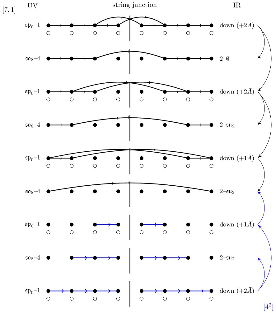
(a) An example of a configuration that was not found for long quivers: partitions $\mu_{L}=[7,1]$, $\mu_{R}=[4^{2}]$ for a short quiver with $9$ curves. Note that two $\overline{A}$’s land on the third $-4$ curve, one from the top (left partition) and one from the bottom (right partition). There, the gauge group is reduced according to $\mathfrak{so}_{7}\overset{\overline{A}}{\rightarrow}\mathfrak{g}_{2}\overset{\overline{A}}{\rightarrow}\mathfrak{su}_{3}$.

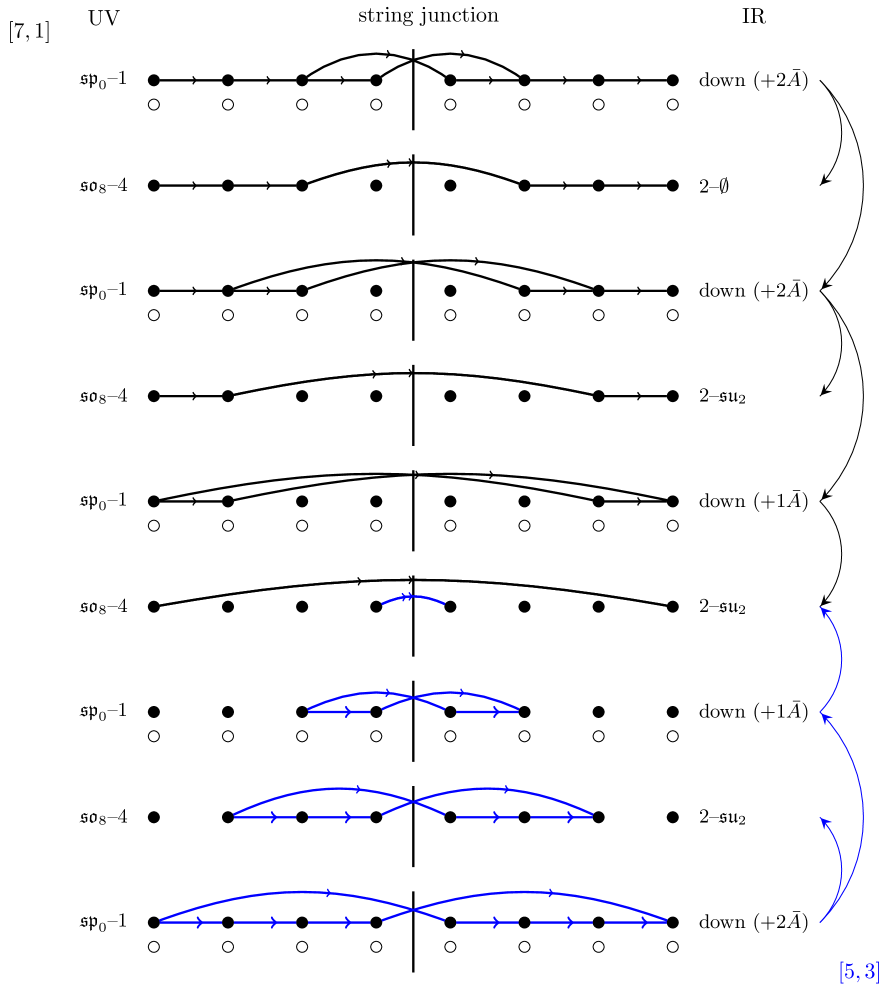
(b) A second example of a configuration that was not found for long quivers: partitions $\mu_{L}=[7,1]$, $\mu_{R}=[5,3]$ for a short quiver with $9$ curves. Note that two $\overline{A}$’s land on the third $-4$ curve, one from the top (left partition) and one from the bottom (right partition). There, the gauge group is reduced according to $\mathfrak{so}_{6}\simeq\mathfrak{su}_{4}\overset{\overline{A}}{\rightarrow}\mathfrak{su}_{3}\overset{\overline{A}}{\rightarrow}\mathfrak{su}_{2}$.

Figure 42: Two interesting examples where two $\overline{A}$’s land on the same $-4$ curve resulting in a chain of Higgsings that was not previously observed for long quivers.

The second novelty is that, in the $SO(8)$ case, partitions related by the triality outer automorphism do not necessarily yield the same IR theory! We saw previously that the long quivers for $\mu=[2^{4}]^{I,II}$ and $\mu=[3,1^{5}]$ are identical, as well as long quivers with deformations $\mu=[4^{2}]^{I,II}$ and $\mu=[5,1^{3}]$. In the case of a long quiver, both of the $[4^{2}]$ and $[5,1^{3}]$ deformations reduces the UV theory to the following IR theory [22]:

$$\overset{\mathfrak{su}(2)}{2}\,\,\underset{[SU(2)]}{\overset{\mathfrak{so}(7)}{3}}\,\,1\,\,\overset{\mathfrak{so}(8)}{4}\dots[SO(8)]\,.$$ (5.21)

However, if we go to the short quiver cases from a UV theory of three $-4$ curves, we see that the pairs of $[4^{2}]$ – $[4^{2}]$ and $[4^{2}]$ – $[5,1^{3}]$ both yield the following quiver theory:

$$\underset{[N_{f}=1/2]}{\overset{\mathfrak{su}(2)}{2}}\,\,\underset{[Sp(2)]}{{\overset{\mathfrak{g_{2}}}{2}}}\,\,\underset{[N_{f}=1/2]}{\overset{\mathfrak{su}(2)}{2}}\,.$$ (5.22)

However, the pair of deformation $[5,1^{3}]$ – $[5,1^{3}]$ gives a different short quiver theory:

$${\overset{\mathfrak{su}(2)}{2}}\,\,\underset{[SU(4)]}{{\overset{\mathfrak{su}(4)}{2}}}\,\,{\overset{\mathfrak{su}(2)}{2}}\,.$$ (5.23)

This is a new effect regarding the outer automorphism of $SO(8)$, which is specific to having a short quiver. The main point is that is that both $[4^{2}]$ – $[4^{2}]$ and $[4^{2}]$ – $[5,1^{3}]$ have one or two $\overline{A}$ branes involved, making it possible to reduce the gauge symmetry to $\mathfrak{g}_{2}$, while the $[5,1^{3}]$ – $[5,1^{3}]$ does not involve $\overline{A}$ branes. Instead, the strings break the UV gauge group down to $\mathfrak{so}(6)\simeq\mathfrak{su}(4)$.

These phenomena are recorded in figures 45, 46, and 47, but we show explicitly the string junction pictures in figure 43 for the partitions $\mu_{L}=\mu_{R}=[4^{2}]$ vs. the partitions $\mu_{L}=\mu_{R}=[5,1^{3}]$. In section 5.2.2, we will justify this surprising conclusion by an analysis of the anomaly polynomials for these respective theories.

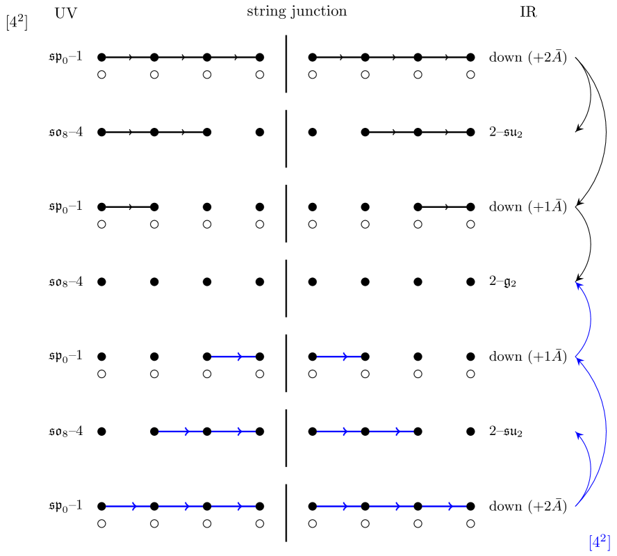
(a) Partitions $\mu_{L}=\mu_{R}=[4^{2}]$ for a short quiver with $7$ curves. We note that in contrast to long quivers, we obtain a different IR theory than for the partitions $\mu_{L}=\mu_{R}=[5,1^{3}]$. Two $\overline{A}$’s land on the middle $-4$ curve, one from the top (left partition) and one from the bottom (right partition). There, the gauge group is reduced according to $\mathfrak{so}_{8}\overset{\overline{A}}{\rightarrow}\mathfrak{so}_{7}\overset{\overline{A}}{\rightarrow}\mathfrak{g}_{2}$.

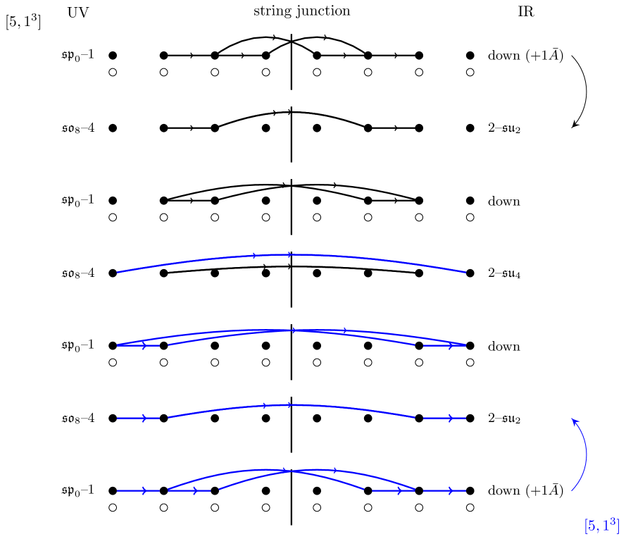
(b) Partitions $\mu_{L}=\mu_{R}=[5,1^{3}]$ for a short quiver with $7$ curves. We note that in contrast to long quivers we obtain a different IR theory than for the partitions $\mu_{L}=\mu_{R}=[4^{2}]$. On the middle $-4$ curve we now have $\mathfrak{so}_{6}\simeq\mathfrak{su}_{4}$ gauge algebra.

Figure 43: Nilpotent orbits with $\mu=[5,1^{3}]$ or $\mu=[4^{2}]$ yield the same IR theories for long quivers (see figure 33 for instance). However, here we see a clear difference for short quivers.

5.1.4 $SO($odd$)$ Case

In general, $SO(2N-1)$ short quivers can be reinterpreted as $SO(2N+2)$ short quivers deformed by a pair of nilpotent orbits. For example, suppose we start from an $SO(7)$ short quiver UV theory, written as:

$$[SO(7)]\ \ 1\ \ \overset{\mathfrak{so}(9)}{4}\ \ \underset{[N_{f}=1]}{\overset{\mathfrak{sp}(1)}{1}}\ \ \overset{\mathfrak{so}(9)}{4}\ \ 1\ \ [SO(7)].$$ (5.24)

This can be reinterpreted as starting from the following $SO(10)$ UV theory:

$$[SO(10)]\ \ \overset{\mathfrak{sp}(1)}{1}\ \ \overset{\mathfrak{so}(10)}{4}\ \ \overset{\mathfrak{sp}(1)}{1}\ \ \overset{\mathfrak{so}(10)}{4}\ \ \overset{\mathfrak{sp}(1)}{1}\ \ [SO(10)],$$ (5.25)

and applying the pair of nilpotent deformations $[3,1^{7}]$ – $[3,1^{7}]$.

In general, any $SO(2N-p)$ quiver with deformations parametrized by the partitions $\mu_{L}^{\mathrm{odd}}$, $\mu_{R}^{\mathrm{odd}}$ of $2N-p$ can be reinterpreted as an $SO(2N)$ quiver with associated partitions $\mu_{L}^{\mathrm{even}}$, $\mu_{R}^{\mathrm{even}}$ obtained by simply adding a “$p$” to the partitions $\mu_{L}^{\mathrm{odd}}$ and $\mu_{R}^{\mathrm{odd}}$, respectively. For instance, for the minimal choice $p=3$ with $\mu_{L}^{\mathrm{odd}}=[1^{9}]$, $\mu_{R}^{\mathrm{odd}}=[7,1^{2}]$, we can equivalently express the theory as an $SO(12)$ quiver with $\mu_{L}^{\mathrm{even}}=[3,1^{9}]$, $\mu_{R}^{\mathrm{even}}=[7,3,1^{2}]$. In this way, the rules we developed for $SO(2N)$ quivers above carry over straightforwardly to $SO(2n-p)$ quivers for $p$ odd.

5.1.5 $Sp$ Case

We now turn to quiver-like theories in which the flavor symmetries are a pair of $Sp$-type. The first thing we should note is that no blow-downs can happen. As a result, there are no “kissing” or “crumpled” configurations. The only constraint that needs to be imposed comes from the Hanany-Witten moves:

$$N_{T}\geq\textrm{Max}\{\mu_{L}^{1},\mu_{R}^{1}\},$$ (5.26)

with $N_{T}$ the number of tensor multiplets in the UV theory.

The behavior of the $Sp$ short quivers is then the same as for $SO(2N)$, where the contributions from each side can overlap, but without any of the complications found due to small instanton transitions or anti-branes. Indeed, no anti-branes are necessary for $Sp$ – $Sp$ quivers.

5.1.6 Mixed $[G]$–$[G^{\prime}]$ Case

It is interesting to consider mixed quivers where the left and right flavors are not equal. The advantage of our analysis is that it straightforwardly generalizes to these cases. Indeed, without loss of generality let $M\leq N$, then

• Quivers with $SU(M)$ – $SU(N)$, $M<N$, flavor symmetries are obtained from partitions of $N$ with $\mu_{L}=[\nu_{L}^{i},N-M]$ and $\mu_{R}=[\mu_{R}^{i}]$, where $[\nu_{L}^{i}]$ is a partition of $M$.

• Quivers with $SO(2M)$ – $SO(2N)$, $M<N$, flavor symmetries are similarly obtained from partitions of $2N$ with $\mu_{L}=[\nu_{L}^{i},(N-M)^{2}]$ and $\mu_{R}=[\mu_{R}^{i}]$, where $[\nu_{L}^{i}]$ is a partition of $2M$.

• Quivers with $SO(\mathrm{even})$ – $Sp$ flavors can be viewed as two $SO(\mathrm{even})$ flavor symmetries with the right most $-1$ curve decompactified. Small instanton transitions of the interior $-1$ curves on the right-hand side of this quiver are allowed only if the resulting base is given by 223 or 23.

• Any quiver involving $SO($odd$)$ flavor symmetries can be embedded inside an $SO($even$)$ quiver, as seen in subsection 5.1.4. Thus, these reduce to the cases above.

5.2 Anomaly Matching for Short Quivers

In this subsection, we propose a method for computing the anomalies of short quivers with classical algebras. We begin by introducing the notion of a “formal $SO$ quiver.” We then show how these can be useful in determining the true F-theory quiver of a 6D SCFT via anomaly polynomial matching. In some cases of short quivers, there is a mismatch between the anomaly polynomial computed via the formal $SO$ quiver and the quiver obtained through the string junction picture described previously. However, this mismatch seems to take a universal form, indicating that the string junction approach may nonetheless give the correct answer, even when there is a disagreement with the formal quiver approach. We conclude the subsection with illustrative examples.

5.2.1 Formal $SO$ theories

“Formal” $SO$ quivers involve analytically continuing the gauge algebra $SO(8+m)$ or $Sp(n)$ so that $m,n\leq 0$. This is only an intermediate step, and the motivation for introducing such formal quiver is to help determine the actual F-theory quiver via anomaly polynomial matching (see [37] for a detailed construction of such formal quivers). Here, we present a brief review of how this is done.

We start from the long quiver case, where we make a comparison between a long $SO(8)$ quiver theory and its formal quiver theory and show that the the anomaly polynomials between the two agree. The actual F-theory quiver is obtained by a $[5,3]$ deformation to the left:

$$[5,3]:\,\,\overset{\mathfrak{su}(2)}{2}\,\,\overset{\mathfrak{g}_{2}}{3}\,\,1\,\,\overset{\mathfrak{so}(8)}{4}\,\,\cdots\,\,1\,\,[SO(8)]\,\,:[1^{8}]\,.$$ (5.27)

On the other hand, we can also express this in terms of a formal quiver by allowing for gauge groups with negative rank:

$$[5,3]:\,\,\overset{\mathfrak{sp}(-3)}{1}\,\,\overset{\mathfrak{so}(4)}{4}\,\,\overset{\mathfrak{sp}(-1)}{1}\,\,\overset{\mathfrak{so}(7)}{4}\,\,1\,\,\overset{\mathfrak{so}(8)}{4}\,\,\cdots\,\,1\,\,[SO(8)]\,\,:[1^{8}]\,.$$ (5.28)

If we truncate both of these theories, keeping only the part of the quiver to the left of the “$\cdots$”, then their anomaly polynomials are both given by

$$I_{8}=\frac{6337}{168}c_{2}(R)^{2}+\frac{25}{336}c_{2}(R)p_{1}(T)+\frac{631}{40320}p_{1}(T)^{2}-\frac{79}{1440}p_{2}(T).$$ (5.29)

In the case of the formal quiver, this anomaly polynomial computation is performed by analytically continuing the formula for an $Sp-SO$ quiver to negative gauge group rank (see [37]).

This example illustrates the utility of the formal quiver for anomaly matching. In our short quiver theories, the actual F-theory quivers can be difficult to read off, whereas these formal $SO$ quivers are easy to determine. As a result, we can use them together with their associated anomaly polynomials relation to check our proposal for the F-theory quiver, as described below.

The general formula for formal quivers–both long and short–is similar to the formula (5.9) for the $SU$ case. Define the partition of the left and right nilpotent orbits of $SO(2N)$ to be $\mu_{L}^{j},\mu_{R}^{j}$ and define their conjugate partitions $\rho_{L}^{j},\rho_{R}^{j}$. We have an alternating sequence of $SO$ and $Sp$ gauge algebras on the full tensor branch. Indexing the gauge algebras by a parameter $m$ which starts with $Sp(q_{1})$ on the left and continues to $SO(p_{2})$, … and terminating with an $Sp$ factor, we have the assignments:

$$SO(p_{m}),~{}~{}~{}p_{m}=2N-\sum_{i=m+1}^{N_{L}^{\prime}}\rho_{i}^{L}-\sum_{j=N_{T}-m+2}^{N_{R}^{\prime}}\rho_{j}^{R}\quad(m\,\,\mathrm{even})$$ (5.30)

$$Sp(q_{m}),~{}~{}~{}q_{m}=\frac{1}{2}(2N-\sum_{i=m+1}^{N_{L}^{\prime}}\rho_{i}^{L}-\sum_{j=N_{T}-m+2}^{N_{R}^{\prime}}\rho_{j}^{R})-4\quad(m\,\,\mathrm{odd})\,.$$ (5.31)

Here, $N_{T}$ is the number of tensor multiplets in the UV F-theory description and $N_{L}^{{}^{\prime}},N_{R}^{{}^{\prime}}$ are the lengths of left and right conjugate partitions, respectively.

Let us illustrate the construction of short quiver formal $SO$ theories by starting with a sufficiently long formal theory and then reducing the length. Consider the $SO(8)$ theory with $[5,3]$ and $[3^{2},1^{2}]$ nilpotent deformations and four $-4$ curves, so that the pair of deformations does not overlap:

$$[5,3]:\,\,\overset{\mathfrak{sp}(-3)}{1}\,\,\overset{\mathfrak{so}(4)}{4}\,\,\overset{\mathfrak{sp}(-1)}{1}\,\,\overset{\mathfrak{so}(7)}{4}\,\,1\,\,\overset{\mathfrak{so}(8)}{4}\,\,1\,\,\overset{\mathfrak{so}(4)}{4}\,\,\overset{\mathfrak{sp}(-1)}{1}\,\,:[3^{2},1^{2}]\,.$$ (5.32)

Now we decrease the length of the quiver. In each step, we start from a shorter UV theory by removing one group of $(-1,-4)$ curves. We get the following set of theories after each step:

$$[5,3]:\,\,\overset{\mathfrak{sp}(-3)}{1}\,\,\overset{\mathfrak{so}(4)}{4}\,\,\overset{\mathfrak{sp}(-1)}{1}\,\,\overset{\mathfrak{so}(7)}{4}\,\,1\,\,\overset{\mathfrak{so}(4)}{4}\,\,\overset{\mathfrak{sp}(-1)}{1}\,\,:[3^{2},1^{2}]$$ (5.33)

$$[5,3]:\,\,\overset{\mathfrak{sp}(-3)}{1}\,\,\overset{\mathfrak{so}(4)}{4}\,\,{\overset{\mathfrak{sp}(-1)}{1}}\,\,\overset{\mathfrak{so}(5)}{4}\,\,{\overset{\mathfrak{sp}(-2)}{1}}\,\,:[3^{2},1^{2}]\,.$$ (5.34)

We stop at this point, following the constraints from the Hanany-Witten moves. We see that the formal gauge algebra goes down to the unphysical values of $\mathfrak{sp}(-3)$ and $\mathfrak{so}(2)$.

However, from such a quiver we may still extract its anomaly polynomial by analytically continuing the formulae developed in the physical regime, $\mathfrak{sp}(m),m>0$ and $\mathfrak{so}(n),n\geq 8$. In the long quiver case, the anomaly polynomial of the formal quiver exactly matches that of the actual quiver [37], as in the example in (5.27)-(5.29). This serves as a strong motivation for us to test the relationship between $SO$ short quivers and their formal counterparts via anomaly matching.

5.2.2 Anomaly Polynomial Matching and Correction Terms

For theories with long quivers, there is a well-defined prescription in the literature for producing the F-theory quiver of a given formal type IIA quiver (see [37]). For short quiver theories, however, the situation becomes much more complicated, and there is at present no well-defined proposal in the literature. Nonetheless, the rules we have introduced in section 4 carry over to the case of short quivers, so we may check that these rules give the correct answer by comparing the anomaly polynomials of the proposed short quiver theories to those obtained from the formal quiver. This check has been done explicitly for all cases in the catalogs LABEL:table:SO8tangentialShortQuiver and LABEL:table:SO10TangentshortQuiver in Appendix C.

In general, we find that there is frequently a mismatch in the $p_{1}(T)^{2}$ and $p_{2}(T)$ coefficients of the anomaly polynomials computed via the formal quiver vs. the actual F-theory quiver. However, this is not very concerning, as the mismatch can always be canceled by adding an appropriate number of neutral hypermultiplets, each of which contributes $(4p_{1}(T)^{2}-7p_{2}(T))/5760$ to the anomaly polynomial. Indeed, such a mismatch in short quiver theories was previously noted in [30].

More concerning are the mismatches in the coefficients of the $c_{2}(R)^{2}$ coefficient and the $c_{2}(R)p_{1}(T)$ coefficient (denoted $\alpha$ and $\beta$, respectively). These mismatches are relatively rare, arising only in a smaller number of kissing cases (see tables LABEL:table:SO8tangentialShortQuiver and LABEL:table:SO10TangentshortQuiver in Appendix C). This could be an indication that these theories are sick and should be discarded. However, we note that these mismatches seem to follow a universal set of rules, which indicates that our proposed F-theory quiver may nonetheless represent an accurate translation of the formal quiver.

Theories with mismatches always involve two anti-branes acting on a curve carrying an $\mathfrak{so}$ gauge algebra according to the rules in (4.6), and it depends on the size of the gauge group. In particular, denoting the mismatch in the anomaly polynomial coefficients $\alpha$ and $\beta$ by $\Delta\alpha$, $\Delta\beta$, respectively, we have:

1. $$\mathfrak{so}(8)\overset{2\overline{A}}{\rightarrow}\mathfrak{g}_{2}:(\Delta\alpha,\Delta\beta)=(0,0)$$ (5.35)

   (see figure 43(a) for an example)

2. $$\mathfrak{so}(7)\overset{2\overline{A}}{\rightarrow}\mathfrak{su}(3):(\Delta\alpha,\Delta\beta)=(\frac{1}{24},\frac{1}{48})$$ (5.36)

   (see figure 42(a) for an example)

3. $$\mathfrak{so}(6)\simeq\mathfrak{su}(4)\overset{2\overline{A}}{\rightarrow}\mathfrak{su}(2):(\Delta\alpha,\Delta\beta)=(\frac{1}{12},\frac{1}{24})$$ (5.37)

   (see figure 42(b) for an example)

4. $$\mathfrak{so}(5)\overset{2\overline{A}}{\rightarrow}\mathfrak{su}(1):(\Delta\alpha,\Delta\beta)=(\frac{1}{6},\frac{1}{12})$$ (5.38)

5. $$\textrm{All remaining cases}:(\Delta\alpha,\Delta\beta)=(0,0).$$ (5.39)

Note that the kissing condition and Hanany-Witten constraints only allow one $-4$ curve to have 2 $\overline{A}$’s simultaneously attach to the curve. There is one borderline case involving $\mathfrak{so}(4)$ gauge symmetry and a pair of $\overline{A}$’s. In both long and short quivers, we have a consistent rule $\mathfrak{so}(4)\overset{\overline{A}}{\rightarrow}\mathfrak{su}(2)$, but adding an additional $\overline{A}$ brane appears to be problematic in general. Including this case would generate a curve without any gauge symmetry, which in many examples leads to a quiver where the “convexity condition” required of gauge group ranks is violated. This is best illustrated with an example. Consider the UV quiver:

$$[1^{16}]\,\,\overset{\mathfrak{sp}(4)}{1}\,\,\overset{\mathfrak{so}(16)}{4}\,\,\overset{\mathfrak{sp}(4)}{1}\,\,\overset{\mathfrak{so}(16)}{4}\,\,\overset{\mathfrak{sp}(4)}{1}\,\,\overset{\mathfrak{so}(16)}{4}\,\,\overset{\mathfrak{sp}(4)}{1}\,\,[1^{16}]$$

If we were to naïvely assume that $\mathfrak{so}(4)\overset{2\overline{A}}{\rightarrow}\emptyset$ without crumpling, then the deformation $\mu_{L}=\mu_{R}=[7^{2},1^{2}]$ would yield the following sick IR theory:

$$[7^{2},1^{2}]\,\,\overset{\mathfrak{su}(2)}{2}\,\,\overset{\emptyset}{2}\,\,\overset{\mathfrak{su}(2)}{2}\,\,[7^{2},1^{2}]$$

From this, we conclude that whenever $\mathfrak{so}(4)$ is hit by two $\overline{A}$’s simultaneously, it must crumple, so we forbid these configurations.

In summary, in cases without a double $\overline{A}$ Higgsing chain (“All remaining cases”) we never have such a mismatch, and in many cases with a double $\overline{A}$ Higgsing chain, there is also no mismatch. There are a few cases where there is a mismatch, which always involve two $\overline{A}$’s in the Higgsing chain. The above proposal has been explicitly verified in the $SO(8)$ and $SO(10)$ catalogs of Appendix C.

What is the physical interpretation of these mismatches? We note that in case (1), where there is no mismatch, the gauge group is reduced from $\mathfrak{so}(8)\overset{2\overline{A}}{\rightarrow}\mathfrak{g}_{2}$, and the brane picture and the string junction root system make perfect sense. However, when there is a mismatch (as in cases (2)-(5)), we always start from an SO brane picture with an orientifold and somehow end up with a SU brane without an orientifold. We leave further explanation of this issue for future work.

5.2.3 Examples

In this section, we present a number of examples to demonstrate our procedure of anomaly matching explicitly and to reveal some of the subtleties of our procedure regarding different quiver lengths, different UV gauge groups, and different types of Higgsing.

• Example 1

  We start with the pair of orbits $[5,1^{3}],[5,1^{3}]$ on an $SO(8)$ UV theory with tensor branch given by three $-4$ curves. The resulting description in F-theory is:

  $$\overset{\mathfrak{su}(2)}{2}\,\,\underset{[SU(4)]}{\overset{\mathfrak{su}(4)}{2}}\,\,\overset{\mathfrak{su}(2)}{2}$$ (5.40)

  This theory gives the same anomaly polynomial as the corresponding formal $SO$ quiver:

  $$[5,1^{3}]:\,\,\overset{\mathfrak{sp}(-2)}{1}\,\,\overset{\mathfrak{so}(5)}{4}\,\,\overset{\mathfrak{sp}(-1)}{1}\,\,\overset{\mathfrak{so}(6)}{4}\,\,\overset{\mathfrak{sp}(-1)}{1}\,\,\overset{\mathfrak{so}(5)}{4}\,\,\overset{\mathfrak{sp}(-2)}{1}\,\,:[5,1^{3}]\,.$$ (5.41)

  The anomaly polynomial reads:

  $$I_{8}=\frac{77}{4}c_{2}(R)^{2}-\frac{3}{8}c_{2}(R)p_{1}(T)+\frac{73}{2880}p_{1}(T)^{2}-\frac{49}{720}p_{2}(T).$$ (5.42)

• Example 2

  For a second example, we deform the UV theory of three $-4$ curves by the pair of orbits of $[4^{2}],[4^{2}]$ (our analysis does not distinguish between the two nilpotent orbits associated with this partition). The formal theory:

  $$[4^{2}]:\,\,\overset{\mathfrak{sp}(-3)}{1}\,\,\overset{\mathfrak{so}(4)}{4}\,\,\overset{\mathfrak{sp}(-1)}{1}\,\,{\overset{\mathfrak{so}(8)}{4}}\,\,\overset{\mathfrak{sp}(-1)}{1}\,\,\overset{\mathfrak{so}(4)}{4}\,\,\overset{\mathfrak{sp}(-3)}{1}\,\,:[4^{2}]$$ (5.43)

  gives the following anomaly polynomial:

  $$\frac{463}{24}c_{2}(R)^{2}-\frac{17}{48}c_{2}(R)p_{1}(T)+\frac{73}{2880}p_{1}(T)^{2}-\frac{101}{1440}p_{2}(T).$$ (5.44)

  If we subtract off the contribution of one neutral hypermultiplet $I_{\textrm{neutral}}=\frac{7p_{1}(T)^{2}-4p_{2}(T)}{5760}$, we get the F-theory quiver anomaly polynomial:

  $$I_{F}=I_{\textrm{formal}}-I_{\textrm{neutral}}=\frac{463}{24}c_{2}(R)^{2}-\frac{17}{48}c_{2}(R)p_{1}(T)+\frac{139}{5760}p_{1}(T)^{2}-\frac{97}{1440}p_{2}(T)$$ (5.45)

  which can be obtained from the F-theory quiver:

  $$[4^{2}]:\,\,\underset{[N_{f}=1/2]}{\overset{\mathfrak{su}(2)}{2}}\,\,\underset{[Sp(2)]}{\overset{\mathfrak{g}_{2}}{2}}\,\,\underset{[N_{f}=1/2]}{\overset{\mathfrak{su}(2)}{2}}\,\,:[4^{2}].$$ (5.46)

  This result is actually quite surprising: the nilpotent deformations considered in these past two examples are related by triality of $SO(8)$. Indeed, their long F-theory quivers are identical, and they have identical anomaly polynomials, even though their formal quivers differ. However, we have just seen that their kissing cases actually differ! We have confirmed this surprising result via anomaly polynomial matching.

• Example 3

  Next, we consider a pair of cases with an anomaly polynomial mismatch.

  • 3a

    Consider the theory with $\mu_{L}=[7,1]$, $\mu_{R}=[4^{2}]$ on an SO(8) UV quiver with four $-4$ curves. The brane pictures for this example are depicted in figure 42(a). The theory has the following IR quiver:

    $$[7,1]:\,\,2\,\,\underset{[N_{f}=1/2]}{\overset{\mathfrak{su}(2)}{2}}\,\,\underset{[SU(2)]}{\overset{\mathfrak{su}(3)}{2}}\,\,\underset{[N_{f}=1]}{\overset{\mathfrak{su}(2)}{2}}\,\,:[4^{2}]\,.$$ (5.47)

    The curve carrying $SU(3)$ naïvely has $\mathfrak{so}(7)$ gauge algebra, but it is hit by two $\overline{A}$’s, one from the right and one from the left. As a result, the gauge algebra is reduced according to $\mathfrak{so}(7)\overset{2\overline{A}}{\rightarrow}\mathfrak{su}(3)$. This puts us in the situation of rule 2, shown in (5.36), so we expect an anomaly correction term of the form $(\Delta\alpha,\Delta\beta)=(1/24,1/48)$.

    Indeed, the formal quiver in this case is given by

    $$[7,1]:\,\,\overset{\mathfrak{sp}(-3)}{1}\,\,\overset{\mathfrak{so}(3)}{4}\,\,\overset{\mathfrak{sp}(-2)}{1}\,\,\overset{\mathfrak{so}(5)}{4}\,\,\overset{\mathfrak{sp}(-1)}{1}\,\,{\overset{\mathfrak{so}(7)}{4}}\,\,\overset{\mathfrak{sp}(-1)}{1}\,\,\overset{\mathfrak{so}(4)}{4}\,\,\overset{\mathfrak{sp}(-3)}{1}\,\,:[4^{2}]\,.$$ (5.48)

    The anomaly polynomial of the F-theory quiver is given by

    $$I_{F}=\frac{1331}{60}c_{2}(R)^{2}-\frac{5}{24}c_{2}(R)p_{1}(T)+\frac{37}{1440}p_{1}(T)^{2}-\frac{31}{360}p_{2}(T),$$ (5.49)

    which is indeed the same as $I_{\textrm{formal}}-c_{2}(R)^{2}/24-c_{2}(R)p_{1}(T)/48-2I_{\textrm{neutral}}$.

  • 3b

    Consider the $SO(8)$ theory with nilpotent deformations $[3,2^{2},1]$ and $[2^{4}]$ on a UV quiver with a single $-4$ curve. The F-theory quiver is given by:

    $$[3,2^{2},1]:\,\,\underset{[SU(6)]}{\overset{\mathfrak{su}(3)}{2}}\,\,:[2^{4}]\,.$$ (5.50)

    Here, we again have one anti-brane from both the left and the right, which collide on the $-4$ curve and reduce it as $\mathfrak{so}(7)\overset{2\overline{A}}{\rightarrow}\mathfrak{su}(3)$. The formal quiver is given by

    $$[3,2^{2},1]:\,\,\overset{\mathfrak{sp}(-2)}{1}\,\,\overset{\mathfrak{so}(7)}{4}\,\,\overset{\mathfrak{sp}(-2)}{1}\,\,:[2^{4}]\,.$$ (5.51)

    The anomaly polynomial of the F-theory quiver is given by

    $$I_{F}=\frac{47}{24}c_{2}(R)^{2}-\frac{7}{48}c_{2}(R)p_{1}(T)+\frac{31}{1920}p_{1}(T)^{2}-\frac{13}{480}p_{2}(T)\,,$$ (5.52)

    which is equal to $I_{\textrm{formal}}-c_{2}(R)^{2}/24-c_{2}(R)p_{1}(T)/48-4I_{\textrm{neutral}}$, as expected from (5.36).

  Note that the rule from (5.36) has worked correctly for both examples, despite the difference in size of their respective quivers.

• Example 4

  As a final example, let us consider a pair of theories with a similar mismatch in the anomaly polynomial but different UV gauge groups.

  • 4a

    First, we consider the theory with $SO(8)$ UV gauge groups, nilpotent deformations $[7,1]$ and $[5,3]$, and a theory with four $-4$ curves, whose brane diagrams are depicted in figure 42(b). The IR quiver takes the form:

    $$[7,1]:\,\,2\,\,\underset{[N_{f}=3/2]}{\overset{\mathfrak{su}(2)}{2}}\,\,{\overset{\mathfrak{su}(2)}{2}}\,\,{\overset{\mathfrak{su}(2)}{2}}\,\,[SU(2)\times SU(2)]\,\,:[5,3]\,.$$ (5.53)

    Here, the middle $\mathfrak{su}(2)$ gauge algebra comes from two anti-branes acting on an $\mathfrak{so}(6)$. Per rule 3 of (5.37), we expect a mismatch of the form $(\Delta\alpha,\Delta\beta)=(1/12,1/24)$. Indeed, the formal quiver is given by

    $$[7,1]:\,\,\overset{\mathfrak{sp}(-3)}{1}\,\,\overset{\mathfrak{so}(3)}{4}\,\,\overset{\mathfrak{sp}(-2)}{1}\,\,\overset{\mathfrak{so}(5)}{4}\,\,\overset{\mathfrak{sp}(-1)}{1}\,\,{\overset{\mathfrak{so}(6)}{4}}\,\,\overset{\mathfrak{sp}(-1)}{1}\,\,\overset{\mathfrak{so}(4)}{4}\,\,\overset{\mathfrak{sp}(-3)}{1}\,\,:[5,3]\,.$$ (5.54)

    The anomaly polynomial of the F-theory quiver is given by

    $$I_{F}=\frac{1943}{120}c_{2}(R)^{2}-\frac{5}{48}c_{2}(R)p_{1}(T)+\frac{47}{1920}p_{1}(T)^{2}-\frac{41}{480}p_{2}(T),$$ (5.55)

    which is indeed the same as $I_{\textrm{formal}}-c_{2}(R)^{2}/12-c_{2}(R)p_{1}(T)/24-2I_{\textrm{neutral}}$.

  • 4b

    Finally, consider the $SO(10)$ theory with nilpotent deformations $[5^{2}]$, $[3^{2},2^{2}]$ on a quiver with two $-4$ curves. This gives:

    $$[5^{2}]:\,\,[SU(2)]\,\,{\overset{\mathfrak{su}(2)}{2}}\,\,{\overset{\mathfrak{su}(2)}{2}}\,\,[SU(2)\times SU(2)]\,\,:[3^{2},2^{2}]\,.$$ (5.56)

    The $\mathfrak{su}(2)$ gauge algebra on the right-hand side again comes from two anti-branes acting on $\mathfrak{so}(6)$. The formal quiver is given by

    $$[5^{2}]:\,\,\overset{\mathfrak{sp}(-3)}{1}\,\,\overset{\mathfrak{so}(4)}{4}\,\,\overset{\mathfrak{sp}(-1)}{1}\,\,\overset{\mathfrak{so}(6)}{4}\,\,\overset{\mathfrak{sp}(-2)}{1}\,\,:[3^{2},2^{2}]\,.$$ (5.57)

    The anomaly polynomial of the F-theory quiver is given by

    $$I_{F}=\frac{23}{6}c_{2}(R)^{2}-\frac{1}{12}c_{2}(R)p_{1}(T)+\frac{11}{720}p_{1}(T)^{2}-\frac{2}{45}p_{2}(T),$$ (5.58)

    which is indeed the same as $I_{\textrm{formal}}-c_{2}(R)^{2}/12-c_{2}(R)p_{1}(T)/24-4I_{\textrm{neutral}}$, as expected from (5.37).

  Note that the rule from (5.37) has worked correctly for both examples, despite the difference in size of their respective quivers as well as their UV gauge groups.

Further examples of anomaly polynomial matching can be found in the catalogs in Appendix C.

5.3 Nilpotent Hierarchy of Short Quivers

Using our analysis above, we now determine a partial ordering for 6D SCFTs based on pairs of nilpotent orbits, which works in both long and short quivers. We refer to this as a “double Hasse diagram,” since it generalizes the independent Hasse diagrams realized by nilpotent orbits on each side of a long quiver (see [22, 70]) to the case of a short quiver, where the nilpotent deformations overlap. We will see that as we reduce the length of the quiver, several nilpotent orbits will end up generating the same IR fixed point. Said another way, different pairs of nilpotent orbits actually give rise to the same IR theory.

Constructing the double Hasse diagrams proceeds in two steps. First we apply the product order to the tuple of left and right partitions $\mu_{L}$ and $\mu_{R}$. It is defined by $(\mu_{L},\mu_{R})\preceq(\nu_{L},\nu_{R})$ which holds if and only if $\mu_{L}\preceq\nu_{L}$ and $\mu_{R}\preceq\nu_{R}$. However, because several deformations in the UV can flow to the same IR theory, we refine this partial ordering in the second step by merging all partitions which result in the same IR quiver. We obtain the same result from a microscopic perspective by appropriately adding strings to the left and right sides of the string junction picture, exactly as we did for the long quivers.

5.3.1 Example: $SU(4)$

As a first example, we consider an $SU(4)$ double Hasse diagram. We begin with the UV theory:

$$[1^{4}]:\underset{[SU(4)]}{\overset{\mathfrak{su}(4)}{2}}\,\overset{\mathfrak{su}(4)}{2}\,\underset{[SU(4)]}{\overset{\mathfrak{su}(4)}{2}}\,\,:[1^{4}]\,.$$ (5.59)

Then we turn on nilpotent deformations on both sides, as in the single-sided versions that were plotted in [22]. Note that $SU(4)$ only has five nilpotent orbits - $[1^{4}],[2,1^{2}],[2^{2}],[3,1],[4]$, but the $[4]$ orbit is prohibited on $N_{-2}=N_{T}=3$ curves by the Hanany-Witten moves constraint of equation (5.2). We are then left with the double Hasse diagram of figure 44. This generalizes straightforwardly to all $SU(N)$ quivers.

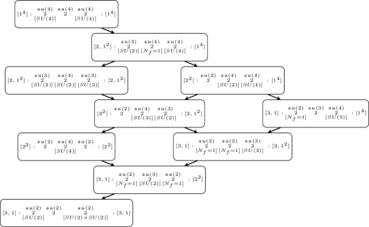
Figure 44: Half of the double Hasse diagram of $SU(4)$ short quivers. The full diagram is obtained by reflection across the left-most nodes, as the quivers can always be flipped under the reflection $\mu_{L}\leftrightarrow\mu_{R}$.

5.3.2 Example: $SO(8)$

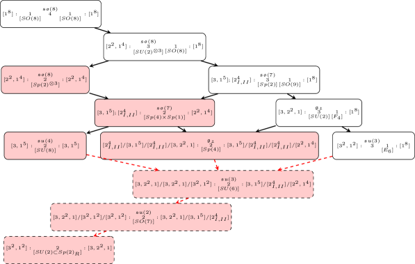
Figure 45: Double Hasse diagram for $SO(8)$ short quiver theories with one $-4$ curve in the UV theory. This diagram is again half of a full figure, following the same convention as in figure 44. “Kissing” configurations are highlighted in red. For concision, several pairs of nilpotent deformations that yield the same IR theory are written in the same box. We separate partitions with semicolons $\mu_{L}$; $\nu_{L}$ – $\mu_{R}$; $\nu_{R}$ to denote all possible combinations $\mu_{L}$ – $\mu_{R}$, $\mu_{L}$ – $\nu_{R}$, $\nu_{L}$ – $\mu_{R}$, and $\nu_{L}$ – $\nu_{R}$. On the other hand, slashes denote one-to-one pairings, so $\mu_{L}/\nu_{L}$ – $\mu_{R}/\nu_{R}$ means $\mu_{L}$ – $\mu_{R}$ and $\nu_{L}$ – $\nu_{R}$ only. We also mark theories with $(\Delta\alpha,\Delta\beta)$ anomaly mismatches with dashed frames and draw the RG flows towards these cases using red dashed arrows. Note that, whenever there is a dashed frame with more than one possible pair of nilpotent orbits, at least one pair of nilpotent orbits out of them has $(\Delta\alpha,\Delta\beta)$ anomaly mismatch, and in some cases not all of them have such mismatches. See table LABEL:table:SO8tangentialShortQuiver for more details of anomaly mismatches in $SO(8)$ short quiver theories.

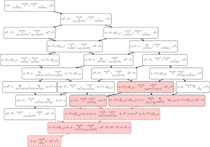
Figure 46: Double Hasse diagram of $SO(8)$ short quiver theories over two $-4$ curves in the UV theory. The notation is the same as in figure 45.

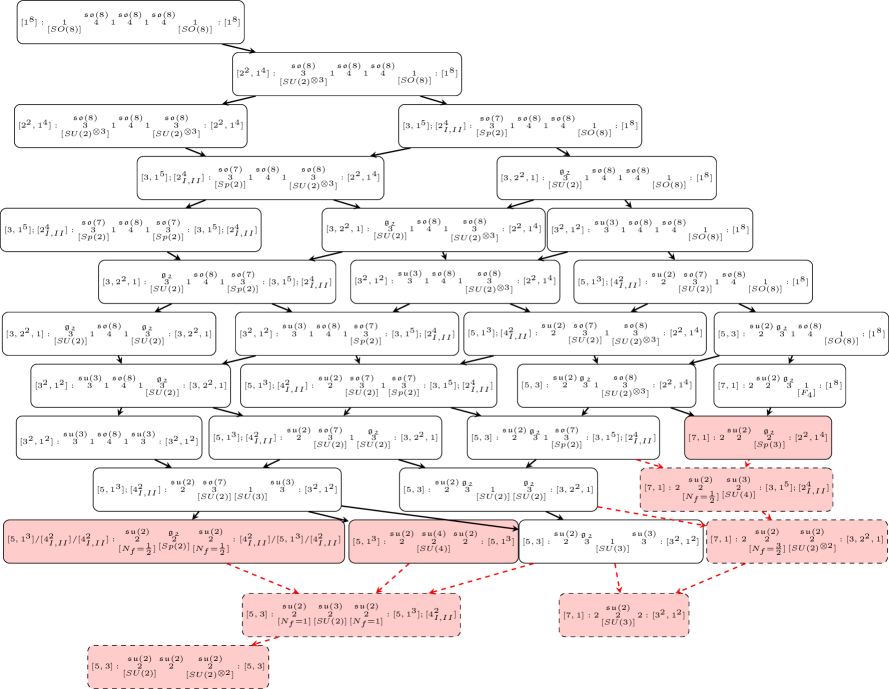
Figure 47: Double Hasse diagram of $SO(8)$ short quiver theories over three $-4$ curves in the UV theory. The notation is the same as in figure 45.

Next we look at the double Hasse diagrams for the $SO(8)$ UV theories. For $SO(2N),N>4$ the story is similar, but we choose to illustrate with $SO(8)$ for simplicity. We look at UV quivers with one, two and three $-4$ curves respectively:

$$[1^{8}]:\underset{[SO(8)]}{1}\, {\overset{\mathfrak{so}(8)}{4}}\,\underset{[SO(8)]}{1}\,:[1^{8}]$$ (5.60)

$$[1^{8}]:\underset{[SO(8)]}{1}\,{\overset{\mathfrak{so}(8)}{4}}\ 1\,{\overset{\mathfrak{so}(8)}{4}}\,\underset{[SO(8)]}{1}\,:[1^{8}]$$ (5.61)

$$[1^{8}]:\underset{[SO(8)]}{1}\,{\overset{\mathfrak{so}(8)}{4}}\,1\, {\overset{\mathfrak{so}(8)}{4}}\,1\,{\overset{\mathfrak{so}(8)}{4}}\,\underset{[SO(8)]}{1}\,:[1^{8}]\,.$$ (5.62)

The associated double Hasse diagrams are shown in figures 45, 46, and 47. We see that as the number of curves decreases, the Hanany-Witten constraints forbid more and more deformations that were allowed in the long quiver. In each diagram, we highlight in red the “kissing” configurations which have all of their $-1$ curves blown-down. We also use dashed lines to indicate theories with an anomaly polynomial mismatch with their associated formal quiver, and we denote flows to these theories with dashed lines.

It is worth pausing here to elaborate on a surprising point noted in example 2 of section 5.2.3 above: $SO(8)$ nilpotent orbits related by triality always give the same long quiver theory, but they do not not always generate the same short quiver theory. When they do yield the same quiver they are drawn in the same box, but when they give rise to distinct theories, we use separate boxes to denote them.

As an example in which the two disagree, consider the short quivers $[3,1^{5}]$ – $[3,1^{5}]$ and $[2^{4}]$ – $[3,1^{5}]$ on a UV quiver with a single $-4$ curve. These yield respectively,

$$[3,1^{5}]:\,\,\overset{\mathfrak{su}_{4}}{2}\,\,[SU(8)]\,\,:[3,1^{5}],$$ (5.63)

$$[2^{4}]:\,\,\overset{\mathfrak{g}_{2}}{2}\,\,[Sp(4)]\,\,:[3,1^{5}]\,.$$ (5.64)

For the first case, with $[3,1^{5}]$ – $[3,1^{5}]$, there are two double strings stretching on the middle curve, so the original $\mathfrak{so}_{8}$ is Higgsed to $\mathfrak{so}_{6}\simeq\mathfrak{su}_{4}$. On the other hand the quiver with $[2^{4}]$ – $[3,1^{5}]$ has a single double string stretching on the middle curve (coming from the right deformation) and one extra $\overline{A}$ coming from the left, so the original $\mathfrak{so}_{8}$ is Higgsed to $\mathfrak{so}_{7}\overset{\overline{A}}{\rightarrow}\mathfrak{g}_{2}$.

The rules that lead us to these quivers can be verified in other examples as well. For instance, consider an $SO(10)$ theory with three $-4$ curves in the UV quiver, deformed by $\mu_{L}=[7,1^{3}]$, $\mu_{R}=[5,3,1^{2}]$. The resulting theory is given by

$$[7,1^{3}]:{\overset{\mathfrak{su}(2)}{2}}\,\,\underset{[SU(4)]}{{\overset{\mathfrak{su}(4)}{2}}}\,\,{\overset{\mathfrak{su}(2)}{2}}:[5,3,1^{2}]\,.$$ (5.65)

In the brane picture, the $\mathfrak{su}(4)$ on the middle $-2$ curve comes from two double strings, one each from the left and right, exactly parallel to the $[3,1^{5}],[3,1^{5}]$ case above.

Similarly, for $\mu_{L}=[7,3]$, $\mu_{R}=[5,3,1^{2}]$, the kissing theory is given by

$$\underset{[N_{f}=1/2]}{\overset{\mathfrak{su}(2)}{2}}\,\,\underset{[Sp(2)]}{{\overset{\mathfrak{g_{2}}}{2}}}\,\,\underset{[N_{f}=1/2]}{\overset{\mathfrak{su}(2)}{2}}\,.$$ (5.66)

The second $-2$ curve now has a $\mathfrak{g}_{2}$ gauge algebra, which in the brane picture comes from a single double string coming from one side and an extra $\overline{A}$ coming from the other, just as in the case of the $[2^{4}]$, $[3,1^{5}]$ theory above.

This example nicely illustrates the utility of the string junction approach for determining the nilpotent hierarchy of short quivers, as the short quivers in two cases (which are different) cannot be determined unambiguously from their associated long quivers alone (which are identical).

Finally, it is also worth noting that additional RG flows have opened up in these short quivers that were not available in the case of long quivers. For instance, in an $SO(8)$ long quiver of fixed size, there is no RG flow from the theory with $\mu_{L}=[3,2^{2},1],\mu_{R}=[1^{8}]$ to the theory with $\mu^{\prime}_{L}=\mu^{\prime}_{R}=[2^{4}]$, because although $\mu_{R}\preceq\mu_{R}^{\prime}$, we also have $\mu_{L}\npreceq\mu_{L}^{\prime}$.

However, for a sufficiently-short quiver with these nilpotent orbits, there is a flow from the former to the latter. In particular, there is a flow from

$$[3,2^{2},1]:\underset{[Sp(1)]}{{\overset{\mathfrak{g}_{2}}{3}}}\,\,\underset{[F_{4}]}{1}:[1^{8}]$$ (5.67)

to the theory

$$[2^{4}]:\underset{[Sp(4)]}{{\overset{\mathfrak{g}_{2}}{2}}}:[2^{4}].$$ (5.68)

This is related to the fact that short quivers are often degenerate: in particular, the theory of (5.68) can also be realized by the nilpotent orbits $\mu_{L}^{\prime}=[3,2^{2},1]$, $\mu_{R}^{\prime}=[2^{2},1^{4}]$, which do satisfy $\mu_{R}\preceq\mu_{R}^{\prime}$, $\mu_{L}\preceq\mu_{L}^{\prime}$.

5.4 Flavor Symmetries

The structure of nilpotent orbits also provides a helpful guide to the analysis of flavor symmetries in 6D SCFTs [22]. Given a nilpotent orbit, the commutant subalgebra specifies an unbroken symmetry inherited from the UV. For the classical groups, the resulting flavor symmetry algebra associated with a given nilpotent orbit is given simply in terms of the data of partition (see e.g. [61]):

$$\begin{array}[]{l@{\quad\text{when}\ }l}\mathfrak{s}[\oplus_{i}\mathfrak{u}(r_{i})]&\mathfrak{g}=\operatorname{\mathit{su}}(N),\\ \displaystyle{\mathop{\mbox{\large$\oplus$}}_{i\,\text{odd}}}\mathfrak{so}(r_{i})\oplus\displaystyle{\mathop{\mbox{\large$\oplus$}}_{i\,\text{even}}}\mathfrak{sp}(r_{i}/2)&\mathfrak{g}=\mathfrak{so}(2N+1)\,\text{or}\,\mathfrak{so}(2N),\\ \displaystyle{\mathop{\mbox{\large$\oplus$}}_{i\,\text{odd}}}\mathfrak{sp}(r_{i}/2)\oplus\displaystyle{\mathop{\mbox{\large$\oplus$}}_{i\,\text{even}}}\mathfrak{so}(r_{i})&\mathfrak{g}=\mathfrak{sp}(N).\\ \end{array}$$ (5.69)

In a long quiver, the flavor symmetry inherited from the parent UV theory is thus given by the products of these flavor symmetries. For short quivers, on the other hand, we typically observe enhancements of the flavor symmetry whenever flavors coming from the left and from the right end up sharing the same node. As usual, this is easiest to see in theories with $\mathfrak{su}$ gauge symmetries. Here, if flavor symmetries $[SU(m)]_{L}$ and $[SU(n)]_{R}$ share the same node, the symmetry enhances from $[SU(m)]\times[SU(n)]$ to $[SU(m+n)]$. For $SO/Sp$ quivers without any small instanton transitions, flavor symmetries of $[SO(m)]_{L}$ and $[SO(n)]_{R}$ get enhanced to $[SO(m+n)]$, and similarly for the $Sp$ cases. To illustrate this fact, we start with the theory

$$[3,2]:\,\,\overset{\mathfrak{su}(2)}{2}\,\,\underset{[N_{f}=1]}{\overset{\mathfrak{su}(4)}{2}}\,\,\underset{[N_{f}=1]}{\overset{\mathfrak{su}(5)}{2}}\,\,\underset{[SU(2)]}{\overset{\mathfrak{su}(5)}{2}}\,\,\underset{[N_{f}=1]}{\overset{\mathfrak{su}(3)}{2}}\,\,:[2^{2},1]\,.$$ (5.70)

We can then shorten the quiver to have only $4$ curves:

$$[3,2]:\,\,\overset{\mathfrak{su}(2)}{2}\,\,\underset{[N_{f}=1]}{\overset{\mathfrak{su}(4)}{2}}\,\,\underset{[SU(3)]}{\overset{\mathfrak{su}(5)}{2}}\,\,\underset{[N_{f}=1]}{\overset{\mathfrak{su}(3)}{2}}\,\,:[2^{2},1].$$ (5.71)

After this first step, we already see an enhancement: the $[SU(3)]$ factor comes from two components: $SU(2)$ from the left and $U(1)$ from the right. Removing yet another curve, we have:

$$[3,2]:\,\,\overset{\mathfrak{su}(2)}{2}\,\,\underset{[SU(3)]}{\overset{\mathfrak{su}(4)}{2}}\,\,\underset{[SU(2)]}{\overset{\mathfrak{su}(3)}{2}}\,\,:[2^{2},1].$$ (5.72)

Here the enhancement is even greater. Indeed, both of the $[SU(3)]$ and $[SU(2)]$ flavors come from similar enhancements.

Ignoring Abelian factors, enhancements occur in the following two cases:

• When flavor symmetries coming from the left and from the right end up sharing the same node.

• When a $-1$ curve has its surrounding gauge symmetry lowered by short quiver effects (as detailed below). This can happen either for a $-1$ at the edge of the quiver or in the interior.

As a first example of the former, consider the theory with nilpotent orbits $[3,1^{5}]$ and $[2^{4}]$ on an $SO(8)$ UV quiver with two $-4$ curves:

$$\underset{[Sp(4)]}{\overset{\mathfrak{g_{2}}}{2}}.$$ (5.73)

We see that the flavor symmetry $Sp(2)\times Sp(2)$ present in the case of a long quiver has been enhanced to $Sp(4)$.

As another example of the former case, consider the theory with nilpotent orbits $\mu_{L}=\mu_{R}=[3,1^{2N-3}]$ on an $SO(2N)$ quiver with one $-4$ curve, which can equivalently be regarded as an $SO(2N-3)$ quiver with $\mu_{L}=\mu_{R}=[1^{2N-3}]$:

$$[SO(2N-2)]\ \ \overset{\mathfrak{sp}(N-5)}{1}\ \ \overset{\mathfrak{so}(2N-2)}{4}\ \ \overset{\mathfrak{sp}(N-5)}{1}\ \ [SO(2N-2)]\,.$$ (5.74)

We see that the flavor symmetries of the left and right have been enhanced from $SO(2N-3)$ to $SO(2N-2)$.

Finally, as an example of the latter case, consider the theory of nilpotent orbits $[7,1]$ and $[1^{8}]$ on an $SO(8)$ UV quiver with three $-4$ curves:

$$2\,\overset{\mathfrak{su}(2)}{2}\,{\overset{\mathfrak{g_{2}}}{3}}\,{1}\,\,[F_{4}].$$ (5.75)

The flavor symmetry on the right has been enhanced from $SO(8)$ to $F_{4}$.

In all cases, we find that the flavor symmetry of a short quiver is enhanced relative to the flavor symmetry of a long quiver associated with the same nilpotent deformations.

6 Conclusions

In this paper we have developed general methods for determining the structure of Higgs branch RG flows in 6D SCFTs. In particular, we have analyzed several aspects of vevs for “conformal matter.” We have seen that the entire nilpotent cone of a simple Lie algebra, including its structure as a partially ordered set can be obtained from simple combinatorial data connected with string junctions stretched between bound states of $7$-branes. Recombination moves involving intersecting branes as well as brane / anti-brane pairs fully determine the Higgs branch of quiver-like 6D SCFTs with classical gauge algebras. An added benefit of this approach is that it also extends to short quiver-like theories where Higgsing from different nilpotent orbits leads to correlated symmetry breaking constraints. In the remainder of this section we discuss some other potential areas for future investigation.

In this paper we have primarily focused on Higgsing in quiver-like theories with classical algebras. We have also seen that we can understand the nilpotent cone of the E-type algebras using multi-pronged string junctions. This suggests that by including additional $7$-brane recombination effects, it should be possible to cover these cases as well. This would provide a nearly complete picture of Higgs branch flows for 6D SCFTs engineered via F-theory.

This work has primarily focused on the case of 6D SCFTs in which Higgs branch deformations can be understood in terms of localized T-brane deformations of a non-compact $7$-brane. We have already noted how “semi-simple” deformations fit into this picture. The other class of Higgs branch deformations which appear quite frequently involve discrete group homomorphisms from finite subgroups of $SU(2)$ into $E_{8}$ [5, 39, 40]. Obtaining an analogous correspondence in this case would cover another broad class of Higgs branch deformations in 6D SCFTs.

The main emphasis of this work has centered on combinatorial data connected with Higgs branch flows and $7$-brane recombination. That being said, it is also clear that explicit complex structure deformations of the associated F-theory models should describe some of these deformations as well, a point which deserves to be clarified.

Lastly, the overarching aim in this work has been to better understand the structure of all possible 6D RG flows obtained from deformations of different conformal fixed points. The fact that we now have a fairly systematic way to also understand deformations of short quivers suggests that the time may be ripe to obtain a full classification of such RG flows.

Appendix A Partial Ordering for Nilpotent Orbits

In this Appendix, we review some aspects of nilpotent orbits of simple Lie algebras and their partial ordering. We refer the interested reader to [71] for further details.

The general linear group $GL(N,\mathbb{C})$ acts on its Lie algebra $\mathfrak{gl}_{n}$ of all complex $n\times n$ matrices by conjugation; the orbits are similarity classes of matrices. The theory of the Jordan form gives a satisfactory parametrization of these classes and allows us to regard two kinds of classes as distinguished: those represented by diagonal matrices, and those represented by strictly upper triangular matrices, i.e., nilpotent matrices. There are only finitely many similarity classes of nilpotent matrices, which are labeled by partitions of of $n$. There is a similar parametrization of nilpotent orbits by partitions in any classical semisimple Lie algebra, with some additional restrictions imposed.

Semi-simple orbits are parametrized by points in a fundamental domain for the action of the Weyl group on a Cartan subalgebra. In particular, there are infinitely many semi-simple orbits.

A.1 Weighted Dynkin Diagrams

Associated to each nilpotent orbit is a unique (completely invariant) weighted Dynkin diagram [71]. In general, the Dynkin labels $\alpha_{i}(H)$, $1\leq i\leq rank(G)$ of a weighted Dynkin diagram are defined by the commutator relation:

$$[H,X_{i}]=\alpha_{i}(H)X_{i},$$ (A.1)

where the $X_{i}$ are the raising operators corresponding to the positive simple roots of $\mathfrak{g}$, and $H$ is directly constructed from the partition $\mathbf{d}=[d_{1},\cdots,d_{n}]$ associated with the nilpotent orbit as follows:

$$H_{[d_{1},\cdots,d_{n}]}=\begin{pmatrix}D(d_{1})&0&\cdots&0\\ 0&D(d_{2})&\cdots&0\\ \vdots&\vdots&\ddots&\vdots\\ 0&0&\cdots&D(d_{k})\end{pmatrix},$$ (A.2)

where

$$D(d_{i})=\begin{pmatrix}d_{i}-1&0&0&\cdots&0&0\\ 0&d_{i}-3&0&\cdots&0&0\\ 0&0&d_{i}-5&\cdots&0&0\\ \vdots&\vdots&\vdots&\ddots&\vdots&\vdots\\ 0&0&0&\cdots&-d_{i}+3&0\\ 0&0&0&\cdots&0&-d_{i}+1\end{pmatrix}$$ (A.3)

The nilpositive element $X$ in the $\{H,X,Y\}$ Jacobson-Morozov standard triple is then given by:

$$X_{[d_{1},\cdots,d_{n}]}=\begin{pmatrix}J^{+}(d_{1})&0&\cdots&0\\ 0&J^{+}(d_{2})&\cdots&0\\ \vdots&\vdots&\ddots&\vdots\\ 0&0&\cdots&J^{+}(d_{k})\end{pmatrix},$$ (A.4)

where now

$$J^{+}_{i,j}(d_{m}) =\delta_{i+1,j}\sqrt{id_{m}-i^{2}}=\begin{pmatrix}0&\sqrt{d_{m}-1}&0&0&\cdots&0&0\\ 0&0&\sqrt{2d_{m}-4}&0&\cdots&0&0\\ 0&0&0&\sqrt{3d_{m}-9}&\cdots&0&0\\ \vdots&\vdots&\vdots&\ddots&\vdots&\vdots&\vdots\\ 0&0&0&\cdots&0&\sqrt{2d_{m}-4}&0\\ 0&0&0&\cdots&0&0&\sqrt{d_{m}-1}\\ 0&0&0&\cdots&0&0&0\end{pmatrix}$$ (A.5)

and similarly the nilnegative element $Y$ is given by:

$$Y_{[d_{1},\cdots,d_{n}]}=\begin{pmatrix}J^{-}(d_{1})&0&\cdots&0\\ 0&J^{-}(d_{2})&\cdots&0\\ \vdots&\vdots&\ddots&\vdots\\ 0&0&\cdots&J^{-}(d_{k})\end{pmatrix},$$ (A.6)

where $J^{-}=(J^{+})^{\dagger}$ so that $Y=X^{\dagger}$:

$$J^{-}_{i,j}(d_{m})=\delta_{j+1,i}\sqrt{jd_{m}-j^{2}}.$$ (A.7)

Direct matrix multiplication then gives the required commutation relations:

$$[X,Y] =H,$$

$$[H,X] =2X,$$

$$[H,Y] =-2Y.$$ (A.8)

This nilpositive matrix is similar to the nilpotent matrix $X_{\mathcal{O}}$ we used to generate the partition in the first place. Indeed, any two matrices with the same Jordan block decomposition (and therefore corresponding to the same partition) are similar matrices and thus belong to the same nilpotent orbit.

As a summary, the following are equivalent:

• A nilpotent orbit

• A given Bala-Carter label

• A corresponding set of simple roots generating the Levi subalgebra and one or more positive roots ($X_{\alpha_{i}}$) for the distinguished orbits

• A corresponding partition

• An $\{H,X,Y\}$ Jacobson-Morozov standard triple, where $H$ is explicitly built out of the partitions as described above and $X$ is similar to the sum of the $X_{\alpha_{i}}$ specified in our brane diagrams.

• A Weighted Dynkin diagram with weights $\alpha_{i}(H)$ given by the relation $[H,X_{i}]=\alpha_{i}(H)X_{i}$ for $H$ defined above in the standard Jacobson-Morozov triple and the $X_{i}$ being the positive simple roots.

Finally, we remark that the dimension of the orbit is given by:

$$\mathrm{dim}(\mathcal{O})=\mathrm{dim}(\mathfrak{g})-\mathrm{dim}(\mathfrak{g}_{0})-\mathrm{dim}(\mathfrak{g}_{1}),$$ (A.9)

where

$$\mathfrak{g}_{j}=\{Z\in\mathfrak{g}\,|\,[H,Z]=jZ\}.$$ (A.10)

Appendix B Review of Anomaly Polynomial Computations

In this Appendix, we briefly review the computation of the anomaly polynomial $I_{8}$ for any 6D SCFT, as originally developed in [45]. For explicit step-by-step examples of anomaly polynomial computations, we refer the interested reader to section 7.1 of [11].

In a theory with a well-defined tensor branch and conventional matter, the anomaly polynomial can be viewed as a sum of two terms: a 1-loop term and a Green-Schwarz term,

$$I_{8}=I_{\text{1-loop}}+I_{\text{GS}}.$$ (B.1)

The full anomaly polynomial of a 6D SCFT takes the form

$$I_{8} =\alpha c_{2}(R)^{2}+\beta c_{2}(R)p_{1}(T)+\gamma p_{1}(T)^{2}+\delta p_{2}(T)$$

$$+\sum_{i}\left[\mu_{i}\,\mathrm{Tr}F_{i}^{4}+\,\mathrm{Tr}F_{i}^{2}\left(\rho_{i}p_{1}(T)+\sigma_{i}c_{2}(R)+\sum_{j}\eta_{ij}\,\mathrm{Tr}F_{j}^{2}\right)\right].$$ (B.2)

Here, $c_{2}(R)$ is the second Chern class of the $SU(2)_{R}$ symmetry, $p_{1}(T)$ is the first Pontryagin class of the tangent bundle, $p_{2}(T)$ is the second Pontryagin class of the tangent bundle, and $F_{i}$ is the field strength of the $i^{th}$ symmetry, where $i$ and $j$ run over the flavor symmetries of the theory.

The 1-loop term receives contributions from free tensor multiplets, vector multiplets, and hypermultiplets:

$$I_{\text{tensor}}=\frac{c_{2}(R)^{2}}{24}+\frac{c_{2}(R)p_{1}(T)}{48} +\frac{23p_{1}(T)^{2}-116p_{2}(T)}{5760},$$ (B.3)

$$I_{\text{vector}}=-\frac{\mathop{\rm tr}\nolimits_{\text{adj}}F^{4}+6c_{2}(R)\mathop{\rm tr}\nolimits_{\text{adj}}F^{2}+d_{G}c_{2}(R)^{2}}{24} -\frac{\mathop{\rm tr}\nolimits_{\text{adj}}F^{2}+d_{G}c_{2}(R)p_{1}(T)}{48}$$

$$-d_{G}\frac{7p_{1}(T)^{2}-4p_{2}(T)}{5760},$$ (B.4)

$$I_{\text{hyper}}=\frac{\mathop{\rm tr}\nolimits_{\rho}F^{4}}{24}+\frac{\mathop{\rm tr}\nolimits_{\rho}F^{2}p_{1}(T)}{48} +d_{\rho}\frac{7p_{1}(T)^{2}-4p_{2}(T)}{5760}.$$ (B.5)

Here, $\mathop{\rm tr}\nolimits_{\rho}$ is the trace in the representation $\rho$, $d_{\rho}$ is the dimension of the representation $\rho$, and $d_{G}$ is the dimension of the group $G$. In computing the anomaly polynomial, one should convert the traces in general representations to the trace in a defining representation. One may write

$$\mathop{\rm tr}\nolimits_{\rho}F^{4}=x_{\rho}\,\mathrm{Tr}F^{4}+y_{\rho}(\,\mathrm{Tr}F^{2})^{2}$$ (B.6)

$$\mathop{\rm tr}\nolimits_{\rho}F^{2}=\text{Ind}_{\rho}\,\mathrm{Tr}F^{2},$$ (B.7)

with $x_{\rho}$, $y_{\rho}$, and $\text{Ind}_{\rho}$ well-known constants in group theory, which can be found in the Appendix of [45] or [11]. For the adjoint representation, $\text{Ind}_{\rho}$ is also known as the dual Coxeter number, $h_{G}^{\vee}$. Note that the groups $SU(2)$, $SU(3)$, $G_{2}$, $F_{4}$, $E_{6}$, $E_{7}$, and $E_{8}$ do not have an independent quartic Casimir $\,\mathrm{Tr}F^{4}$, so $x_{\rho}=0$ for all representations of these groups.

The Green-Schwarz term takes the form

$$I_{\text{GS}}=\frac{1}{2}A^{ij}I_{i}I_{j},$$ (B.8)

where $A^{ij}$ is a negative-definite matrix given by the inverse of the Dirac pairing on the string charge lattice. The term $I_{i}$ can be written as

$$I_{i}=a_{i}c_{2}(R)+b_{i}p_{1}(T)+\sum_{j}c_{ij}\,\mathrm{Tr}F_{j}^{2}.$$ (B.9)

The coefficients $a_{i}$, $b_{i}$, and $c_{ij}$ are chosen so that the gauge anomalies $(\mathrm{Tr}F_{i}^{2})^{2}$ and mixed gauge-gauge or gauge-global anomalies (e.g. $\mathrm{Tr}F_{i}^{2}\mathrm{Tr}F_{j}^{2}$, $\mathrm{Tr}F_{i}^{2}c_{2}(R)$, $\mathrm{Tr}F_{i}^{2}p_{1}(T)$) vanish. In other words, these anomalies must precisely cancel between the Green-Schwarz term and the 1-loop term. In practice, one need not compute the individual $I_{i}$: one can simply complete the square with respect to the quadratic Casimir $\mathrm{Tr}F_{i}^{2}$ of each of the gauge groups in turn. This is guaranteed to cancel out the gauge anomalies and mixed gauge anomalies, and what is left is simply the total anomaly polynomial $I_{8}$.

Appendix C Catalogs of Short Quiver Theories

In this Appendix we present explicit catalogs of “kissing cases” for $SO(8)$ and $SO(10)$ short quiver theories, each under a particular UV gauge group but varying UV length. For each case, we give the exact “kissing case”, together with the “preceding theory” obtained from the nilpotent orbit but with a slightly longer quiver to illustrate how such collisions between the nilpotent deformations take place. As in [30], we may compute the anomaly polynomial of the kissing theory directly, but we can also compute it via analytic continuation from a formal type IIA quiver. In most cases, this procedure gives the same result, but in some cases, there is an additional correction term, which we display in the right-hand columns of the following tables. This additional correction term can also be read off from the brane picture, as explained in section 5.2.2.

Table 2: A catalog for $SO(8)$ kissing short quiver cases, their preceding longer theory, and the relevant terms for anomaly matching. The $\mathcal{O}_{L,R}$ columns correspond to the left and right deformations. Here $\Delta\alpha=\alpha_{\textrm{formal}}-\alpha_{F}$, and likewise for $\Delta\beta$. The “Preceding Theory” column gives the theory whose length is one longer than the kissing theory, under the same pair of nilpotent orbits. The “Theory” column gives the actual deformed short quiver theory, while the $\#I_{n}$ columns stands for the number of anomaly of neutral hypermultiplets to be added to the F-theory quiver in order to match the coefficients $\gamma$ and $\delta$ of the formal quiver. The last entry indicates that there is an $SU(2)\subset Sp(2)_{R}$ flavor symmetry. By this, we mean that the IR theory ends up flowing to a theory with $\mathcal{N}=(2,0)$ supersymmetry, where the R-symmetry group is $Sp(2)_{R}$. Viewed as an $\mathcal{N}=(1,0)$ SCFT, there is an $SU(2)$ flavor symmetry and an $SU(2)_{R}$ R-symmetry.

$\mathcal{O}_{L}$	$\mathcal{O}_{R}$	Preceding Theory	Kissing Theory	$\#I_{n}$	$\Delta\alpha$	$\Delta\beta$
$[7,1]$	$[7,1]$	$2\,\,{{\overset{\mathfrak{su}(2)}{2}}}\,\,{\overset{\mathfrak{g_{2}}}{3}}\,\,\underset{[SU(2)]}{1}\,\,{\overset{\mathfrak{g_{2}}}{3}}\,\,{{\overset{\mathfrak{su}(2)}{2}}}\,\,{2}$	${2}\,\,\underset{[N_{f}=3/2]}{{\overset{\mathfrak{su}(2)}{2}}}\,\,\underset{[SU(2)]}{\overset{\mathfrak{su}(2)}{2}}\,\,\underset{[N_{f}=3/2]}{{\overset{\mathfrak{su}(2)}{2}}}\,\,{2}$	2	$\frac{1}{12}$	$\frac{1}{24}$
$[7,1]$	$[4^{2}]$	$2\,\,{\overset{\mathfrak{su}(2)}{2}}\,\,{{\overset{\mathfrak{g_{2}}}{3}}}\,\,1\,\,\underset{[SU(2)]}{{\overset{\mathfrak{so}(7)}{3}}}\,\,{\overset{\mathfrak{su}(2)}{2}}$	${2}\,\,\underset{[N_{f}=1/2]}{\overset{\mathfrak{su}(2)}{2}}\,\,\underset{[SU(2)]}{{\overset{\mathfrak{su}(3)}{2}}}\,\,\underset{[N_{f}=1]}{\overset{\mathfrak{su}(2)}{2}}$	2	$\frac{1}{24}$	$\frac{1}{48}$
$[7,1]$	$[5,1^{3}]$	$2\,\,{\overset{\mathfrak{su}(2)}{2}}\,\,{{\overset{\mathfrak{g_{2}}}{3}}}\,\,1\,\,\underset{[SU(2)]}{{\overset{\mathfrak{so}(7)}{3}}}\,\,{\overset{\mathfrak{su}(2)}{2}}$	${2}\,\,\underset{[N_{f}=1/2]}{\overset{\mathfrak{su}(2)}{2}}\,\,\underset{[SU(2)]}{{\overset{\mathfrak{su}(3)}{2}}}\,\,\underset{[N_{f}=1]}{\overset{\mathfrak{su}(2)}{2}}$	2	0	0
$[7,1]$	$[5,3]$	$2\,\,{\overset{\mathfrak{su}(2)}{2}}\,\,{{\overset{\mathfrak{g_{2}}}{3}}}\,\,\underset{[SU(2)]}{1}\,\,{\overset{\mathfrak{g_{2}}}{3}}\,\,{\overset{\mathfrak{su}(2)}{2}}$	${2}\,\,\underset{[N_{f}=3/2]}{{\overset{\mathfrak{su}(2)}{2}}}\,\,{\overset{\mathfrak{su}(2)}{2}}\,\,{\overset{\mathfrak{su}(2)}{2}}\,\,[SU(2)\times SU(2)]$	2	$\frac{1}{12}$	$\frac{1}{24}$
$[4^{2}]$	$[4^{2}]$	${\overset{\mathfrak{su}(2)}{2}}\,\,\underset{[SU(2)]}{{\overset{\mathfrak{so}(7)}{3}}}\,\,1\,\,\underset{[SU(2)]}{{\overset{\mathfrak{so}(7)}{3}}}\,\,{\overset{\mathfrak{su}(2)}{2}}$	$\underset{[N_{f}=1/2]}{\overset{\mathfrak{su}(2)}{2}}\,\,\underset{[Sp(2)]}{{\overset{\mathfrak{g_{2}}}{2}}}\,\,\underset{[N_{f}=1/2]}{\overset{\mathfrak{su}(2)}{2}}$	2	0	0
$[5,1^{3}]$	$[4^{2}]$	${\overset{\mathfrak{su}(2)}{2}}\,\,\underset{[SU(2)]}{{\overset{\mathfrak{so}(7)}{3}}}\,\,1\,\,\underset{[SU(2)]}{{\overset{\mathfrak{so}(7)}{3}}}\,\,{\overset{\mathfrak{su}(2)}{2}}$	$\underset{[N_{f}=1/2]}{\overset{\mathfrak{su}(2)}{2}}\,\,\underset{[Sp(2)]}{{\overset{\mathfrak{g_{2}}}{2}}}\,\,\underset{[N_{f}=1/2]}{\overset{\mathfrak{su}(2)}{2}}$	1	0	0
$[5,1^{3}]$	$[5,1^{3}]$	${\overset{\mathfrak{su}(2)}{2}}\,\,\underset{[SU(2)]}{{\overset{\mathfrak{so}(7)}{3}}}\,\,1\,\,\underset{[SU(2)]}{{\overset{\mathfrak{so}(7)}{3}}}\,\,{\overset{\mathfrak{su}(2)}{2}}$	${\overset{\mathfrak{su}(2)}{2}}\,\,\underset{[SU(4)]}{{\overset{\mathfrak{su}(4)}{2}}}\,\,{\overset{\mathfrak{su}(2)}{2}}$	0	0	0
$[5,3]$	$[4^{2}]$	${\overset{\mathfrak{su}(2)}{2}}\,\,{{\overset{\mathfrak{g_{2}}}{3}}}\,\,1\,\,\underset{[SU(2)]}{{\overset{\mathfrak{so}(7)}{3}}}\,\,{\overset{\mathfrak{su}(2)}{2}}$	$\underset{[N_{f}=1]}{\overset{\mathfrak{su}(2)}{2}}\,\,\underset{[SU(2)]}{{\overset{\mathfrak{su}(3)}{2}}}\,\,\underset{[N_{f}=1]}{\overset{\mathfrak{su}(2)}{2}}$	2	$\frac{1}{24}$	$\frac{1}{48}$
$[5,3]$	$[5,1^{3}]$	${\overset{\mathfrak{su}(2)}{2}}\,\,{{\overset{\mathfrak{g_{2}}}{3}}}\,\,1\,\,\underset{[SU(2)]}{{\overset{\mathfrak{so}(7)}{3}}}\,\,{\overset{\mathfrak{su}(2)}{2}}$	$\underset{[N_{f}=1]}{\overset{\mathfrak{su}(2)}{2}}\,\,\underset{[SU(2)]}{{\overset{\mathfrak{su}(3)}{2}}}\,\,\underset{[N_{f}=1]}{\overset{\mathfrak{su}(2)}{2}}$	2	0	0
$[5,3]$	$[5,3]$	${\overset{\mathfrak{su}(2)}{2}}\,\,{\overset{\mathfrak{g_{2}}}{3}}\,\,\underset{[SU(2)]}{1}\,\,{{\overset{\mathfrak{g_{2}}}{3}}}\,\,{\overset{\mathfrak{su}(2)}{2}}$	$[SU(2)\times SU(2)]\,\,{\overset{\mathfrak{su}(2)}{2}}\,\,{\overset{\mathfrak{su}(2)}{2}}\,\,{\overset{\mathfrak{su}(2)}{2}}\,\,[SU(2)]$	2	$\frac{1}{12}$	$\frac{1}{24}$
$[7,1]$	$[2^{2},1^{4}]$	${2}\,\,{\overset{\mathfrak{su}(2)}{2}}\,\,{{\overset{\mathfrak{g_{2}}}{3}}}\,\,1\,\,\underset{[SU(2)^{\otimes 3}]}{{\overset{\mathfrak{so}(8)}{3}}}$	$2\,\,{\overset{\mathfrak{su}(2)}{2}}\,\,{\overset{\mathfrak{g_{2}}}{2}}\,\,[Sp(3)]$	2	0	0
$[7,1]$	$[2^{4}]$	${2}\,\,{\overset{\mathfrak{su}(2)}{2}}\,\,{{\overset{\mathfrak{g_{2}}}{3}}}\,\,1\,\,\underset{[Sp(2)]}{{\overset{\mathfrak{so}(7)}{3}}}$	${2}\,\,\underset{[N_{f}=1/2]}{\overset{\mathfrak{su}(2)}{2}}\,\,{\overset{\mathfrak{su}(3)}{2}}\,\,[SU(4)]$	3	$\frac{1}{24}$	$\frac{1}{48}$
$[7,1]$	$[3,1^{5}]$	${2}\,\,{\overset{\mathfrak{su}(2)}{2}}\,\,{{\overset{\mathfrak{g_{2}}}{3}}}\,\,1\,\,\underset{[Sp(2)]}{{\overset{\mathfrak{so}(7)}{3}}}$	${2}\,\,\underset{[N_{f}=1/2]}{\overset{\mathfrak{su}(2)}{2}}\,\,{\overset{\mathfrak{su}(3)}{2}}\,\,[SU(4)]$	4	0	0
$[7,1]$	$[3,2^{2},1]$	${2}\,\,{\overset{\mathfrak{su}(2)}{2}}\,\,{{\overset{\mathfrak{g_{2}}}{3}}}\,\,\underset{[SU(2)]}{1}\,\,\underset{[SU(2)]}{{\overset{\mathfrak{g_{2}}}{3}}}$	${2}\,\,\underset{[N_{f}=3/2]}{\overset{\mathfrak{su}(2)}{2}}\,\,{\overset{\mathfrak{su}(2)}{2}}\,\,[SU(2)\times SU(2)]$	4	$\frac{1}{12}$	$\frac{1}{24}$
$[7,1]$	$[3^{2},1^{2}]$	${2}\,\,{\overset{\mathfrak{su}(2)}{2}}\,\,{{\overset{\mathfrak{g_{2}}}{3}}}\,\,\underset{[SU(3)]}{1}\,\,{\overset{\mathfrak{su}(3)}{3}}$	${2}\,\,\underset{[SU(3)]}{\overset{\mathfrak{su}(2)}{2}}\,\,2$	4	$\frac{1}{6}$	$\frac{1}{12}$
$[4^{2}]$	$[2^{2},1^{4}]$	${\overset{\mathfrak{su}(2)}{2}}\,\,\underset{[SU(2)]}{\overset{\mathfrak{so}(7)}{3}}\,\,1\,\,\underset{[SU(2)^{\otimes 3}]}{\overset{\mathfrak{so}(8)}{3}}$	${\overset{\mathfrak{su}(2)}{2}}\,\,{\overset{\mathfrak{so}(7)}{2}}\,\,[Sp(3)\times Sp(1)]$	1	0	0
$[4^{2}]$	$[2^{4}]$	${\overset{\mathfrak{su}(2)}{2}}\,\,\underset{[SU(2)]}{\overset{\mathfrak{so}(7)}{3}}\,\,1\,\,\underset{[Sp(2)]}{\overset{\mathfrak{so}(7)}{3}}$	$\underset{[N_{f}=1/2]}{\overset{\mathfrak{su}(2)}{2}}\,\,{\overset{\mathfrak{g_{2}}}{2}}\,\,[Sp(3)]$	3	0	0
$[4^{2}]$	$[3,1^{5}]$	${\overset{\mathfrak{su}(2)}{2}}\,\,\underset{[SU(2)]}{\overset{\mathfrak{so}(7)}{3}}\,\,1\,\,\underset{[Sp(2)]}{\overset{\mathfrak{so}(7)}{3}}$	$\underset{[N_{f}=1/2]}{\overset{\mathfrak{su}(2)}{2}}\,\,{\overset{\mathfrak{g_{2}}}{2}}\,\,[Sp(3)]$	2	0	0
$[4^{2}]$	$[3,2^{2},1]$	${\overset{\mathfrak{su}(2)}{2}}\,\,\underset{[SU(2)]}{\overset{\mathfrak{so}(7)}{3}}\,\,1\,\,\underset{[SU(2)]}{\overset{\mathfrak{g_{2}}}{3}}$	$\underset{[N_{f}=1]}{\overset{\mathfrak{su}(2)}{2}}\,\,{\overset{\mathfrak{su}(3)}{2}}\,\,[SU(4)]$	3	$\frac{1}{24}$	$\frac{1}{48}$
$[4^{2}]$	$[3^{2},1^{2}]$	${\overset{\mathfrak{su}(2)}{2}}\,\,\underset{[SU(2)]}{\overset{\mathfrak{so}(7)}{3}}\,\,\underset{[SU(2)]}{1}\,\,{\overset{\mathfrak{su}(3)}{3}}$	$[SU(2)]\,\,{\overset{\mathfrak{su}(2)}{2}}\,\,{\overset{\mathfrak{su}(2)}{2}}\,\,[SU(2)\times SU(2)]$	4	$\frac{1}{12}$	$\frac{1}{24}$
$[5,1^{3}]$	$[2^{2},1^{4}]$	${\overset{\mathfrak{su}(2)}{2}}\,\,\underset{[SU(2)]}{\overset{\mathfrak{so}(7)}{3}}\,\,1\,\,\underset{[SU(2)^{\otimes 3}]}{\overset{\mathfrak{so}(8)}{3}}$	${\overset{\mathfrak{su}(2)}{2}}\,\,{\overset{\mathfrak{so}(7)}{2}}\,\,[Sp(3)\times Sp(1)]$	0	0	0
$[5,1^{3}]$	$[2^{4}]$	${\overset{\mathfrak{su}(2)}{2}}\,\,\underset{[SU(2)]}{\overset{\mathfrak{so}(7)}{3}}\,\,1\,\,\underset{[Sp(2)]}{\overset{\mathfrak{so}(7)}{3}}$	$\underset{[N_{f}=1/2]}{\overset{\mathfrak{su}(2)}{2}}\,\,{\overset{\mathfrak{g_{2}}}{2}}\,\,[Sp(3)]$	1	0	0
$[5,1^{3}]$	$[3,1^{5}]$	${\overset{\mathfrak{su}(2)}{2}}\,\,\underset{[SU(2)]}{\overset{\mathfrak{so}(7)}{3}}\,\,1\,\,\underset{[Sp(2)]}{\overset{\mathfrak{so}(7)}{3}}$	${\overset{\mathfrak{su}(2)}{2}}\,\,{\overset{\mathfrak{su}(4)}{2}}\,\,[SU(6)]$	0	0	0
$[5,1^{3}]$	$[3,2^{2},1]$	${\overset{\mathfrak{su}(2)}{2}}\,\,\underset{[SU(2)]}{\overset{\mathfrak{so}(7)}{3}}\,\,1\,\,\underset{[SU(2)]}{\overset{\mathfrak{g_{2}}}{3}}$	$\underset{[N_{f}=1]}{\overset{\mathfrak{su}(2)}{2}}\,\,{\overset{\mathfrak{su}(3)}{2}}\,\,[SU(4)]$	2	$0$	$0$
$[5,1^{3}]$	$[3^{2},1^{2}]$	${\overset{\mathfrak{su}(2)}{2}}\,\,\underset{[SU(2)]}{\overset{\mathfrak{so}(7)}{3}}\,\,\underset{[SU(2)]}{1}\,\,{\overset{\mathfrak{su}(3)}{3}}$	$[SU(2)]\,\,{\overset{\mathfrak{su}(2)}{2}}\,\,{\overset{\mathfrak{su}(2)}{2}}\,\,[SU(2)\times SU(2)]$	4	0	0
$[5,3]$	$[2^{2},1^{4}]$	${\overset{\mathfrak{su}(2)}{2}}\,\,{\overset{\mathfrak{g_{2}}}{3}}\,\,1\,\,\underset{[SU(2)^{\otimes 3}]}{\overset{\mathfrak{so}(8)}{3}}$	$\underset{[N_{f}=1/2]}{\overset{\mathfrak{su}(2)}{2}}\,\,{\overset{\mathfrak{g_{2}}}{2}}\,\,[Sp(3)]$	2	0	0
$[5,3]$	$[2^{4}]$	${\overset{\mathfrak{su}(2)}{2}}\,\,{\overset{\mathfrak{g_{2}}}{3}}\,\,1\,\,\underset{[Sp(2)]}{\overset{\mathfrak{so}(7)}{3}}$	$\underset{[N_{f}=1]}{\overset{\mathfrak{su}(2)}{2}}\,\,{\overset{\mathfrak{su}(3)}{2}}\,\,[SU(4)]$	3	$\frac{1}{24}$	$\frac{1}{48}$
$[5,3]$	$[3,1^{5}]$	${\overset{\mathfrak{su}(2)}{2}}\,\,{\overset{\mathfrak{g_{2}}}{3}}\,\,1\,\,\underset{[Sp(2)]}{\overset{\mathfrak{so}(7)}{3}}$	$\underset{[N_{f}=1]}{\overset{\mathfrak{su}(2)}{2}}\,\,{\overset{\mathfrak{su}(3)}{2}}\,\,[SU(4)]$	4	0	0
$[5,3]$	$[3,2^{2},1]$	${\overset{\mathfrak{su}(2)}{2}}\,\,{\overset{\mathfrak{g_{2}}}{3}}\,\,\underset{[SU(2)]}{1}\,\,\underset{[SU(2)]}{\overset{\mathfrak{g_{2}}}{3}}$	$[SU(2)]\,\,{\overset{\mathfrak{su}(2)}{2}}\,\,{\overset{\mathfrak{su}(2)}{2}}\,\,[SU(2)\times SU(2)]$	4	$\frac{1}{12}$	$\frac{1}{24}$
$[5,3]$	$[3^{2},1^{2}]$	${\overset{\mathfrak{su}(2)}{2}}\,\,{\overset{\mathfrak{g_{2}}}{3}}\,\,\underset{[SU(3)]}{1}\,\,{\overset{\mathfrak{su}(3)}{3}}$	$[G_{2}]\,\,{\overset{\mathfrak{su}(2)}{2}}\,\,2$	4	$\frac{1}{6}$	$\frac{1}{12}$
$[2^{2},1^{4}]$	$[2^{2},1^{4}]$	$\underset{[SU(2)^{\otimes 3}]}{\overset{\mathfrak{so}(8)}{3}}\,\,1\,\,\underset{[SU(2)^{\otimes 3}]}{\overset{\mathfrak{so}(8)}{3}}$	${\overset{\mathfrak{so}(8)}{2}}\,\,[Sp(2)\times Sp(2)\times Sp(2)]$	0	0	0
$[2^{4}]$	$[2^{2},1^{4}]$	$\underset{[Sp(2)]}{\overset{\mathfrak{so}(7)}{3}}\,\,1\,\,\underset{[SU(2)^{\otimes 3}]}{\overset{\mathfrak{so}(8)}{3}}$	${\overset{\mathfrak{so}(7)}{2}}\,\,[Sp(4)\times Sp(1)]$	1	0	0
$[3,1^{5}]$	$[2^{2},1^{4}]$	$\underset{[Sp(2)]}{\overset{\mathfrak{so}(7)}{3}}\,\,1\,\,\underset{[SU(2)^{\otimes 3}]}{\overset{\mathfrak{so}(8)}{3}}$	${\overset{\mathfrak{so}(7)}{2}}\,\,[Sp(4)\times Sp(1)]$	0	0	0
$[2^{4}]$	$[2^{4}]$	$\underset{[Sp(2)]}{\overset{\mathfrak{so}(7)}{3}}\,\,1\,\,\underset{[Sp(2)]}{\overset{\mathfrak{so}(7)}{3}}$	${\overset{\mathfrak{g_{2}}}{2}}\,\,[Sp(4)]$	4	0	0
$[3,1^{5}]$	$[2^{4}]$	$\underset{[Sp(2)]}{\overset{\mathfrak{so}(7)}{3}}\,\,1\,\,\underset{[Sp(2)]}{\overset{\mathfrak{so}(7)}{3}}$	${\overset{\mathfrak{g_{2}}}{2}}\,\,[Sp(4)]$	2	0	0
$[3,1^{5}]$	$[3,1^{5}]$	$\underset{[Sp(2)]}{\overset{\mathfrak{so}(7)}{3}}\,\,1\,\,\underset{[Sp(2)]}{\overset{\mathfrak{so}(7)}{3}}$	${\overset{\mathfrak{su}(4)}{2}}\,\,[SU(8)]$	0	0	0
$[3,2^{2},1]$	$[2^{2},1^{4}]$	$\underset{[SU(2)]}{\overset{\mathfrak{g_{2}}}{3}}\,\,1\,\,\underset{[SU(2)^{\otimes 3}]}{\overset{\mathfrak{so}(8)}{3}}$	${\overset{\mathfrak{g_{2}}}{2}}\,\,[Sp(4)]$	2	0	0
$[3,2^{2},1]$	$[2^{4}]$	$\underset{[SU(2)]}{\overset{\mathfrak{g_{2}}}{3}}\,\,1\,\,\underset{[Sp(2)]}{\overset{\mathfrak{so}(7)}{3}}$	${\overset{\mathfrak{su}(3)}{2}}\,\,[SU(6)]$	4	$\frac{1}{24}$	$\frac{1}{48}$
$[3,2^{2},1]$	$[3,1^{5}]$	$\underset{[SU(2)]}{\overset{\mathfrak{g_{2}}}{3}}\,\,1\,\,\underset{[Sp(2)]}{\overset{\mathfrak{so}(7)}{3}}$	${\overset{\mathfrak{su}(3)}{2}}\,\,[SU(6)]$	4	0	0
$[3,2^{2},1]$	$[3,2^{2},1]$	$\underset{[SU(2)]}{\overset{\mathfrak{g_{2}}}{3}}\,\,\underset{[SU(2)]}{1}\,\,\underset{[SU(2)]}{\overset{\mathfrak{g_{2}}}{3}}$	${\overset{\mathfrak{su}(2)}{2}}\,\,[SO(7)]$	6	$\frac{1}{12}$	$\frac{1}{24}$
$[3^{2},1^{2}]$	$[2^{2},1^{4}]$	${\overset{\mathfrak{su}(3)}{3}}\,\,1\,\,\underset{[SU(2)^{\otimes 3}]}{\overset{\mathfrak{so}(8)}{3}}$	${\overset{\mathfrak{su}(3)}{2}}\,\,[SU(6)]$	4	0	0
$[3^{2},1^{2}]$	$[2^{4}]$	${\overset{\mathfrak{su}(3)}{3}}\,\,\underset{[SU(2)]}{1}\,\,\underset{[Sp(2)]}{\overset{\mathfrak{so}(7)}{3}}$	${\overset{\mathfrak{su}(2)}{2}}\,\,[SO(7)]$	6	$\frac{1}{12}$	$\frac{1}{24}$
$[3^{2},1^{2}]$	$[3,1^{5}]$	${\overset{\mathfrak{su}(3)}{3}}\,\,\underset{[SU(2)]}{1}\,\,\underset{[Sp(2)]}{\overset{\mathfrak{so}(7)}{3}}$	${\overset{\mathfrak{su}(2)}{2}}\,\,[SO(7)]$	8	0	0
$[3^{2},1^{2}]$	$[3,2^{2},1]$	${\overset{\mathfrak{su}(3)}{3}}\,\,\underset{[SU(3)]}{1}\,\,\underset{[SU(2)]}{\overset{\mathfrak{g_{2}}}{3}}$	$2\,\,[SU(2)\subset Sp(2)_{R}]$	7	$\frac{1}{6}$	$\frac{1}{12}$

Table 3: $SO(10)$ short quiver tangential cases, in parallel to table LABEL:table:SO8tangentialShortQuiver. See table LABEL:table:SO8tangentialShortQuiver for conventions and notation.

$\mathcal{O}_{L}$	$\mathcal{O}_{R}$	“Preceding Theory”	“Kissing Theory”	$\#I_{n}$	$\Delta\alpha$	$\Delta\beta$
$[9,1]$	$[9,1]$	$2\,\,{\overset{\mathfrak{su}(2)}{2}}\,\,{{\overset{\mathfrak{g}_{2}}{3}}}\,\,1\,\,{\overset{\mathfrak{so}(8)}{4}}\,\,1{\,\,{\overset{\mathfrak{g}_{2}}{3}}}\,\,{\overset{\mathfrak{su}(2)}{2}}\,\,2$	$2\,\,\underset{[N_{f}=1/2]}{\overset{\mathfrak{su}(2)}{2}}\,\,\underset{[N_{f}=1]}{{\overset{\mathfrak{su}(3)}{2}}}\,\,\underset{[N_{f}=1]}{\overset{\mathfrak{su}(3)}{2}}\,\,\underset{[N_{f}=1/2]}{\overset{\mathfrak{su}(2)}{2}}\,\,2$	1	0	0
$[9,1]$	$[7,1^{3}]$	$2\,\,{\overset{\mathfrak{su}(2)}{2}}\,\,{\overset{\mathfrak{g}_{2}}{3}}\,\,1\,\,{\overset{\mathfrak{so}(8)}{4}}\,\ 1\,\,\underset{[SU(2)]}{{\overset{\mathfrak{so}(7)}{3}}}\,\,{\overset{\mathfrak{su}(2)}{2}}$	$2\,\,\underset{[N_{f}=1/2]}{\overset{\mathfrak{su}(2)}{2}}\,\,{\overset{\mathfrak{su}(3)}{2}}\underset{[SU(3)]}{\,\,{\overset{\mathfrak{su}(4)}{2}}}\,\,{\overset{\mathfrak{su}(2)}{2}}$	0	0	0
$[9,1]$	$[7,3]$	$2\,\,{\overset{\mathfrak{su}(2)}{2}}\,\,{\overset{\mathfrak{g}_{2}}{3}}\,\,1\,\,{\overset{\mathfrak{so}(8)}{4}}\,\ 1\,\,{\overset{\mathfrak{g}_{2}}{3}}\,\,{\overset{\mathfrak{su}(2)}{2}}$	$2\,\,\underset{[N_{f}=1/2]}{\overset{\mathfrak{su}(2)}{2}}\,\,\underset{[N_{f}=1]}{{\overset{\mathfrak{su}(3)}{2}}}\,\,\underset{[N_{f}=1]}{{\overset{\mathfrak{su}(3)}{2}}}\,\,\underset{[N_{f}=1]}{\overset{\mathfrak{su}(2)}{2}}$	1	0	0
$[7,1^{3}]$	$[7,1^{3}]$	${\overset{\mathfrak{su}(2)}{2}}\,\,\underset{[SU(2)]}{{\overset{\mathfrak{so}(7)}{3}}}\,\,1\,\,{\overset{\mathfrak{so}(8)}{4}}\,\ 1\,\,\underset{[SU(2)]}{{\overset{\mathfrak{so}(7)}{3}}}\,\,{\overset{\mathfrak{su}(2)}{2}}$	${\overset{\mathfrak{su}(2)}{2}}\,\,\underset{[SU(2)]}{{\overset{\mathfrak{su}(4)}{2}}}\underset{[SU(2)]}{\,\,{\overset{\mathfrak{su}(4)}{2}}}\,\,{\overset{\mathfrak{su}(2)}{2}}$	0	0	0
$[7,3]$	$[7,1^{3}]$	${\overset{\mathfrak{su}(2)}{2}}\,\,{\overset{\mathfrak{g}_{2}}{3}}\,\,1\,\,{\overset{\mathfrak{so}(8)}{4}}\,\ 1\,\,\underset{[SU(2)]}{{\overset{\mathfrak{so}(7)}{3}}}\,\,{\overset{\mathfrak{su}(2)}{2}}$	$\underset{[N_{f}=1]}{\overset{\mathfrak{su}(2)}{2}}\,\,{\overset{\mathfrak{su}(3)}{2}}\,\,\underset{[SU(3)]}{{\overset{\mathfrak{su}(4)}{2}}}\,\,{\overset{\mathfrak{su}(2)}{2}}$	0	0	0
$[7,3]$	$[7,3]$	${\overset{\mathfrak{su}(2)}{2}}\,\,{\overset{\mathfrak{g}_{2}}{3}}\,\,1\,\,{\overset{\mathfrak{so}(8)}{4}}\,\ 1\,\,{\overset{\mathfrak{g}_{2}}{3}}\,\,{\overset{\mathfrak{su}(2)}{2}}$	$\underset{[N_{f}=1]}{\overset{\mathfrak{su}(2)}{2}}\,\,\underset{[N_{f}=1]}{{\overset{\mathfrak{su}(3)}{2}}}\,\,\underset{[N_{f}=1]}{{\overset{\mathfrak{su}(3)}{2}}}\,\,\underset{[N_{f}=1]}{\overset{\mathfrak{su}(2)}{2}}$	1	0	0
$[9,1]$	$[4^{2},1^{2}]$	$2\,\,{\overset{\mathfrak{su}(2)}{2}}\,\,{\overset{\mathfrak{g}_{2}}{3}}\,\,1\,\,\underset{[Sp(1)]}{\overset{\mathfrak{so}(9)}{4}}\,\ 1\,\,{\overset{\mathfrak{su}(3)}{3}}$	$2\,\,{\overset{\mathfrak{su}(2)}{2}}\,\,\underset{[Sp(2)]}{{\overset{\mathfrak{g_{2}}}{2}}}\,\,\underset{[N_{f}=1/2]}{\overset{\mathfrak{su}(2)}{2}}$	1	0	0
$[9,1]$	$[5,1^{5}]$	$2\,\,{\overset{\mathfrak{su}(2)}{2}}\,\,{\overset{\mathfrak{g}_{2}}{3}}\,\,1\,\,{\overset{\mathfrak{so}(8)}{4}}\,\ 1\,\,{\overset{\mathfrak{so}(7)}{3}}\,\,[Sp(2)]$	$2\,\,\underset{[N_{f}=1/2]}{\overset{\mathfrak{su}(2)}{2}}\,\,{\overset{\mathfrak{su}(3)}{2}}\,\,{\overset{\mathfrak{su}(4)}{2}}\,\,[SU(5)]$	0	0	0
$[9,1]$	$[5,2^{2},1]$	$2\,\,{\overset{\mathfrak{su}(2)}{2}}\,\,{\overset{\mathfrak{g}_{2}}{3}}\,\,1\,\,{\overset{\mathfrak{so}(8)}{4}}\,\ 1\,\,\underset{[SU(2)]}{{\overset{\mathfrak{g}_{2}}{3}}}$	$2\,\,\underset{[N_{f}=1/2]}{\overset{\mathfrak{su}(2)}{2}}\,\,\underset{[N_{f}=1]}{{\overset{\mathfrak{su}(3)}{2}}}\,\,{\overset{\mathfrak{su}(3)}{2}}\,\,[SU(3)]$	1	0	0
$[9,1]$	$[5,3,1^{2}]$	$2\,\,{\overset{\mathfrak{su}(2)}{2}}\,\,{\overset{\mathfrak{g}_{2}}{3}}\,\,1\,\,{\overset{\mathfrak{so}(8)}{4}}\,\ 1\,\,{{\overset{\mathfrak{su}(3)}{3}}}$	$2\,\,\underset{[N_{f}=1/2]}{\overset{\mathfrak{su}(2)}{2}}\,\,\underset{[SU(2)]}{{\overset{\mathfrak{su}(3)}{2}}}\,\,\underset{[N_{f}=1]}{\overset{\mathfrak{su}(2)}{2}}$	2	0	0
$[5^{2}]$	$[5^{2}]$	${\overset{\mathfrak{su}(2)}{2}}\,\,{\overset{\mathfrak{so}(7)}{3}}\,\,\underset{[SO(4)]}{{\overset{\mathfrak{sp}(1)}{1}}}\,\,{\overset{\mathfrak{so}(7)}{3}}\,\,{\overset{\mathfrak{su}(2)}{2}}$	$[SU(2)]\,\,{\overset{\mathfrak{su}(2)}{2}}\,\,{{\overset{\mathfrak{su}(2)}{2}}}\,\,{\overset{\mathfrak{su}(2)}{2}}\,\,[SU(2)\times SU(2)]$	2	$\frac{1}{12}$	$\frac{1}{24}$
$[7,1^{3}]$	$[4^{2},1^{2}]$	${\overset{\mathfrak{su}(2)}{2}}\,\,\underset{[SU(2)]}{{\overset{\mathfrak{so}(7)}{3}}}\,\,1\,\,\underset{[Sp(1)]}{\overset{\mathfrak{so}(9)}{4}}\,\ 1\,\,{{\overset{\mathfrak{su}(3)}{3}}}$	${\overset{\mathfrak{su}(2)}{2}}\,\,\underset{[Sp(2)\times Sp(1)]}{{\overset{\mathfrak{so}(7)}{2}}}\,\,{\overset{\mathfrak{su}(2)}{2}}$	0	0	0
$[7,1^{3}]$	$[5,1^{5}]$	${\overset{\mathfrak{su}(2)}{2}}\,\,\underset{[SU(2)]}{{\overset{\mathfrak{so}(7)}{3}}}\,\,1\,\,{\overset{\mathfrak{so}(8)}{4}}\,\ 1\,\,{{\overset{\mathfrak{so}(7)}{3}}}\,\,[Sp(2)]$	${\overset{\mathfrak{su}(2)}{2}}\,\,\underset{[SU(2)]}{{\overset{\mathfrak{su}(4)}{2}}}\,\,{\overset{\mathfrak{su}(4)}{2}}\,\,[SU(4)]$	0	0	0
$[7,1^{3}]$	$[5,2^{2},1]$	${\overset{\mathfrak{su}(2)}{2}}\,\,\underset{[SU(2)]}{{\overset{\mathfrak{so}(7)}{3}}}\,\,1\,\,{\overset{\mathfrak{so}(8)}{4}}\,\ 1\,\,{{\overset{\mathfrak{g}_{2}}{3}}}\,\,[SU(2)]$	${\overset{\mathfrak{su}(2)}{2}}\,\,\underset{[SU(3)]}{{\overset{\mathfrak{su}(4)}{2}}}\,\,{\overset{\mathfrak{su}(3)}{2}}\,\,[SU(2)]$	0	0	0
$[7,1^{3}]$	$[5,3,1^{2}]$	${\overset{\mathfrak{su}(2)}{2}}\,\,\underset{[SU(2)]}{{\overset{\mathfrak{so}(7)}{3}}}\,\,1\,\,{\overset{\mathfrak{so}(8)}{4}}\,\ 1\,\,{{\overset{\mathfrak{su}(3)}{3}}}$	${\overset{\mathfrak{su}(2)}{2}}\,\,\underset{[SU(4)]}{{\overset{\mathfrak{su}(4)}{2}}}\,\,{\overset{\mathfrak{su}(2)}{2}}$	0	0	0
$[7,3]$	$[4^{2},1^{2}]$	${\overset{\mathfrak{su}(2)}{2}}\,\,{\overset{\mathfrak{g}_{2}}{3}}\,\,1\,\,\underset{[Sp(1)]}{\overset{\mathfrak{so}(9)}{4}}\,\ 1\,\,{{\overset{\mathfrak{su}(3)}{3}}}$	$\underset{[N_{f}=1/2]}{\overset{\mathfrak{su}(2)}{2}}\,\,\underset{[Sp(2)]}{{\overset{\mathfrak{g_{2}}}{2}}}\,\,\underset{[N_{f}=1/2]}{\overset{\mathfrak{su}(2)}{2}}$	1	0	0
$[7,3]$	$[5,1^{5}]$	${\overset{\mathfrak{su}(2)}{2}}\,\,{\overset{\mathfrak{g}_{2}}{3}}\,\,1\,\,{\overset{\mathfrak{so}(8)}{4}}\,\ 1\,\,\underset{[Sp(2)]}{{\overset{\mathfrak{so}(7)}{3}}}$	$\underset{[N_{f}=1]}{\overset{\mathfrak{su}(2)}{2}}\,\,{\overset{\mathfrak{su}(3)}{2}}\,\,{\overset{\mathfrak{su}(4)}{2}}\,\,[SU(5)]$	0	0	0
$[7,3]$	$[5,2^{2},1]$	${\overset{\mathfrak{su}(2)}{2}}\,\,{\overset{\mathfrak{g}_{2}}{3}}\,\,1\,\,{\overset{\mathfrak{so}(8)}{4}}\,\ 1\,\,\underset{[SU(2)]}{{\overset{\mathfrak{g}_{2}}{3}}}$	$\underset{[N_{f}=1]}{\overset{\mathfrak{su}(2)}{2}}\,\,\underset{[N_{f}=1]}{{\overset{\mathfrak{su}(3)}{2}}}\,\,{\overset{\mathfrak{su}(3)}{2}}\,\,[SU(3)]$	1	0	0
$[7,3]$	$[5,3,1^{2}]$	${\overset{\mathfrak{su}(2)}{2}}\,\,{\overset{\mathfrak{g}_{2}}{3}}\,\,1\,\,{\overset{\mathfrak{so}(8)}{4}}\,\ 1\,\,{{\overset{\mathfrak{su}(3)}{3}}}$	$\underset{[N_{f}=1]}{\overset{\mathfrak{su}(2)}{2}}\,\,\underset{[SU(2)]}{{\overset{\mathfrak{su}(3)}{2}}}\,\,\underset{[N_{f}=1]}{\overset{\mathfrak{su}(2)}{2}}$	3	0	0
$[4^{2},1^{2}]$	$[4^{2},1^{2}]$	${\overset{\mathfrak{su}(3)}{3}}\,\,1\,\,\underset{[Sp(2)]}{{\overset{\mathfrak{so}(10)}{4}}}\,\,1\,\,{\overset{\mathfrak{su}(3)}{3}}$	$[SU(3)]\,\,{\overset{\mathfrak{su}(3)}{2}}\,\,{\overset{\mathfrak{su}(3)}{2}}\,\,[SU(3)]$	1	0	0
$[5,1^{5}]$	$[4^{2},1^{2}]$	$\underset{[Sp(2)]}{\overset{\mathfrak{so}(7)}{3}}\,\,1\,\,\underset{[Sp(1)]}{\overset{\mathfrak{so}(9)}{4}}\,\,1\,\,{\overset{\mathfrak{su}(3)}{3}}$	$[Sp(3)\times Sp(1)]\,\,{\overset{\mathfrak{so}(7)}{2}}\,\,{\overset{\mathfrak{su}(2)}{2}}$	0	0	0
$[5,1^{5}]$	$[5,1^{5}]$	$\underset{[Sp(2)]}{\overset{\mathfrak{so}(7)}{3}}\,\,1\,\,{\overset{\mathfrak{so}(8)}{4}}\,\,1\,\,\underset{[Sp(2)]}{\overset{\mathfrak{so}(7)}{3}}$	$[SU(4)]\,\,{\overset{\mathfrak{su}(4)}{2}}\,\,{\overset{\mathfrak{su}(4)}{2}}\,\,[SU(4)]$	0	0	0
$[5,2^{2},1]$	$[4^{2},1^{2}]$	$\underset{[SU(2)]}{\overset{\mathfrak{g}_{2}}{3}}\,\,1\,\,\underset{[Sp(1)]}{\overset{\mathfrak{so}(9)}{4}}\,\,1\,\,{\overset{\mathfrak{su}(3)}{3}}$	$[Sp(3)]\,\,{\overset{\mathfrak{g_{2}}}{2}}\,\,\underset{[N_{f}=1/2]}{\overset{\mathfrak{su}(2)}{2}}$	1	0	0
$[5,2^{2},1]$	$[5,1^{5}]$	$\underset{[SU(2)]}{\overset{\mathfrak{g}_{2}}{3}}\,\,1\,\,{\overset{\mathfrak{so}(8)}{4}}\,\,1\,\,\underset{[Sp(2)]}{\overset{\mathfrak{so}(7)}{3}}$	$[SU(2)]\,\,{\overset{\mathfrak{su}(3)}{2}}\,\,{\overset{\mathfrak{su}(4)}{2}}\,\,[SU(5)]$	0	0	0
$[5,2^{2},1]$	$[5,2^{2},1]$	$\underset{[SU(2)]}{\overset{\mathfrak{g}_{2}}{3}}\,\,1\,\,{\overset{\mathfrak{so}(8)}{4}}\,\,1\,\,\underset{[SU(2)]}{\overset{\mathfrak{g}_{2}}{3}}$	$[SU(3)]\,\,{\overset{\mathfrak{su}(3)}{2}}\,\,{\overset{\mathfrak{su}(3)}{2}}\,\,[SU(3)]$	1	0	0
$[5,3,1^{2}]$	$[4^{2},1^{2}]$	${\overset{\mathfrak{su}(3)}{3}}\,\,1\,\,\underset{[Sp(1)]}{\overset{\mathfrak{so}(9)}{4}}\,\,1\,\,{\overset{\mathfrak{su}(3)}{3}}$	$[SU(4)]\,\,{\overset{\mathfrak{su}(3)}{2}}\,\,\underset{[N_{f}=1]}{\overset{\mathfrak{su}(2)}{2}}$	2	0	0
$[5,3,1^{2}]$	$[5,1^{5}]$	${\overset{\mathfrak{su}(3)}{3}}\,\,1\,\,{\overset{\mathfrak{so}(8)}{4}}\,\,1\,\,\underset{[Sp(2)]}{\overset{\mathfrak{so}(7)}{3}}$	${\overset{\mathfrak{su}(2)}{2}}\,\,{\overset{\mathfrak{su}(4)}{2}}\,\,[SU(6)]$	0	0	0
$[5,3,1^{2}]$	$[5,2^{2},1]$	${\overset{\mathfrak{su}(3)}{3}}\,\,1\,\,{\overset{\mathfrak{so}(8)}{4}}\,\,1\,\,\underset{[SU(2)]}{\overset{\mathfrak{g}_{2}}{3}}$	$\underset{[N_{f}=1]}{\overset{\mathfrak{su}(2)}{2}}\,\,{\overset{\mathfrak{su}(3)}{2}}\,\,[SU(4)]$	2	0	0
$[5,3,1^{2}]$	$[5,3,1^{2}]$	${\overset{\mathfrak{su}(3)}{3}}\,\,1\,\,{\overset{\mathfrak{so}(8)}{4}}\,\,1\,\,{\overset{\mathfrak{su}(3)}{3}}$	$[SU(2)]\,\,{\overset{\mathfrak{su}(2)}{2}}\,\,{\overset{\mathfrak{su}(2)}{2}}\,\,[SU(2)\times SU(2)]$	4	0	0
$[5^{2}]$	$[2^{4},1^{2}]$	${\overset{\mathfrak{su}(2)}{2}}\,\,{\overset{\mathfrak{so}(7)}{3}}\,\,\underset{[N_{f}=1]}{\overset{\mathfrak{sp}(1)}{1}}\,\,\underset{[N_{s}=1]}{\overset{\mathfrak{so}(10)}{3}}\,\,[Sp(2)]$	${\overset{\mathfrak{su}(2)}{2}}\,\,{\overset{\mathfrak{so}(7)}{2}}\,\,[Sp(3)\times Sp(1)]$	1	0	0
$[5^{2}]$	$[3,2^{2},1^{3}]$	${\overset{\mathfrak{su}(2)}{2}}\,\,{\overset{\mathfrak{so}(7)}{3}}\,\,\underset{[SO(3)]}{\overset{\mathfrak{sp}(1)}{1}}\,\,\underset{[Sp(1)\times Sp(1)]}{\overset{\mathfrak{so}(9)}{3}}$	$\underset{[N_{f}=1/2]}{\overset{\mathfrak{su}(2)}{2}}\,\,{\overset{\mathfrak{g_{2}}}{2}}\,\,[Sp(3)]$	2	0	0
$[5^{2}]$	$[3^{2},1^{4}]$	${\overset{\mathfrak{su}(2)}{2}}\,\,{\overset{\mathfrak{so}(7)}{3}}\,\,\underset{[SO(4)]}{\overset{\mathfrak{sp}(1)}{1}}\,\,\underset{[Sp(1)\times Sp(1)]}{\overset{\mathfrak{so}(8)}{3}}$	$\underset{[N_{f}=1]}{\overset{\mathfrak{su}(2)}{2}}\,\,{\overset{\mathfrak{su}(3)}{2}}\,\,[SU(4)]$	4	0	0
$[5^{2}]$	$[3^{2},2^{2}]$	${\overset{\mathfrak{su}(2)}{2}}\,\,{\overset{\mathfrak{so}(7)}{3}}\,\,\underset{[SO(4)]}{\overset{\mathfrak{sp}(1)}{1}}\,\,\underset{[Sp(2)]}{\overset{\mathfrak{so}(7)}{3}}$	$[SU(2)]\,\,{\overset{\mathfrak{su}(2)}{2}}\,\,{\overset{\mathfrak{su}(2)}{2}}\,\,[SU(2)\times SU(2)]$	4	$\frac{1}{12}$	$\frac{1}{24}$
$[5^{2}]$	$[3^{3},1]$	${\overset{\mathfrak{su}(2)}{2}}\,\,{\overset{\mathfrak{so}(7)}{3}}\,\,\underset{{[SO(5)]}}{\overset{\mathfrak{sp}(1)}{1}}\,\,{\overset{\mathfrak{g}_{2}}{3}}$	$[G_{2}]\,\,{\overset{\mathfrak{su}(2)}{2}}\,\,2$	4	$\frac{1}{6}$	$\frac{1}{12}$
$[2^{4},1^{2}]$	$[2^{4},1^{2}]$	$[Sp(2)]\,\,\underset{[N_{s}=1]}{\overset{\mathfrak{so}(10)}{3}}\,\,{\overset{\mathfrak{sp}(1)}{1}}\,\,\underset{[N_{s}=1]}{\overset{\mathfrak{so}(10)}{3}}\,\,[Sp(2)]$	${\overset{\mathfrak{so}(10)}{2}}\,\,[Sp(4)\times SU(2)]$	0	0	0
$[3,2^{2},1^{3}]$	$[2^{4},1^{2}]$	$\underset{[Sp(1)\times Sp(1)]}{\overset{\mathfrak{so}(9)}{3}}\,\,\underset{[N_{f}=1/2]}{\overset{\mathfrak{sp}(1)}{1}}\,\,\underset{[N_{s}=1]}{\overset{\mathfrak{so}(10)}{3}}\,\,[Sp(2)]$	${\overset{\mathfrak{so}(9)}{2}}\,\,[Sp(3)\times Sp(2)]$	0	0	0
$[3,2^{2},1^{3}]$	$[3,2^{2},1^{3}]$	$\underset{[Sp(1)\times Sp(1)]}{\overset{\mathfrak{so}(9)}{3}}\,\,\underset{[N_{f}=1]}{\overset{\mathfrak{sp}(1)}{1}}\,\,\underset{[Sp(1)\times Sp(1)]}{\overset{\mathfrak{so}(9)}{3}}$	${\overset{\mathfrak{so}(8)}{2}}\,\,[Sp(2)\times Sp(2)\times Sp(2)]$	0	0	0
$[3^{2},1^{4}]$	$[2^{4},1^{2}]$	$\underset{[Sp(1)\times Sp(1)]}{\overset{\mathfrak{so}(8)}{3}}\,\,\underset{[N_{f}=1]}{\overset{\mathfrak{sp}(1)}{1}}\,\,\underset{[N_{s}=1]}{\overset{\mathfrak{so}(10)}{3}}\,\,[Sp(2)]$	${\overset{\mathfrak{so}(8)}{2}}\,\,[Sp(2)\times Sp(2)\times Sp(2)]$	0	0	0
$[3^{2},1^{4}]$	$[3,2^{2},1^{3}]$	$\underset{[Sp(1)\times Sp(1)]}{\overset{\mathfrak{so}(8)}{3}}\,\,\underset{[SO(3)]}{\overset{\mathfrak{sp}(1)}{1}}\,\,\underset{[Sp(1)\times Sp(1)]}{\overset{\mathfrak{so}(9)}{3}}$	${\overset{\mathfrak{so}(7)}{2}}\,\,[Sp(4)\times Sp(1)]$	0	0	0
$[3^{2},1^{4}]$	$[3^{2},1^{4}]$	$\underset{[Sp(1)\times Sp(1)]}{\overset{\mathfrak{so}(8)}{3}}\,\,\underset{[SO(4)]}{\overset{\mathfrak{sp}(1)}{1}}\,\,\underset{[Sp(1)\times Sp(1)]}{\overset{\mathfrak{so}(8)}{3}}$	${\overset{\mathfrak{su}(4)}{2}}\,\,[SU(8)]$	0	0	0
$[3^{2},2^{2}]$	$[2^{4},1^{2}]$	$\underset{[Sp(1)]}{\overset{\mathfrak{so}(7)}{3}}\,\,\underset{[N_{f}=1]}{\overset{\mathfrak{sp}(1)}{1}}\,\,\underset{[N_{s}=1]}{\overset{\mathfrak{so}(10)}{3}}\,\,[Sp(2)]$	${\overset{\mathfrak{so}(7)}{2}}\,\,[Sp(4)\times Sp(1)]$	1	0	0
$[3^{2},2^{2}]$	$[3,2^{2},1^{3}]$	$\underset{[Sp(1)]}{\overset{\mathfrak{so}(7)}{3}}\,\,\underset{[SO(3)]}{\overset{\mathfrak{sp}(1)}{1}}\,\,\underset{[Sp(1)\times Sp(1)]}{\overset{\mathfrak{so}(9)}{3}}$	${\overset{\mathfrak{g_{2}}}{2}}\,\,[Sp(4)]$	2	0	0
$[3^{2},2^{2}]$	$[3^{2},1^{4}]$	$\underset{[Sp(1)]}{\overset{\mathfrak{so}(7)}{3}}\,\,\underset{[SO(4)]}{\overset{\mathfrak{sp}(1)}{1}}\,\,\underset{[Sp(1)\times Sp(1)]}{\overset{\mathfrak{so}(8)}{3}}$	${\overset{\mathfrak{su}(3)}{2}}\,\,[SU(6)]$	4	0	0
$[3^{2},2^{2}]$	$[3^{2},2^{2}]$	$\underset{[Sp(1)]}{\overset{\mathfrak{so}(7)}{3}}\,\,\underset{[SO(4)]}{\overset{\mathfrak{sp}(1)}{1}}\,\,\underset{[Sp(1)]}{\overset{\mathfrak{so}(7)}{3}}$	${\overset{\mathfrak{su}(2)}{2}}\,\,[SO(7)]$	6	$\frac{1}{12}$	$\frac{1}{24}$
$[3^{3},1]$	$[2^{4},1^{2}]$	${\overset{\mathfrak{g}_{2}}{3}}\,\,\underset{{[SO(3)]}}{\overset{\mathfrak{sp}(1)}{1}}\,\,\underset{[N_{s}=1]}{\overset{\mathfrak{so}(10)}{3}}\,\,[Sp(2)]$	${\overset{\mathfrak{g_{2}}}{2}}\,\,[Sp(4)]$	2	0	0
$[3^{3},1]$	$[3,2^{2},1^{3}]$	${\overset{\mathfrak{g}_{2}}{3}}\,\,\underset{{[SO(4)]}}{\overset{\mathfrak{sp}(1)}{1}}\,\,\underset{[Sp(1)\times Sp(1)]}{\overset{\mathfrak{so}(9)}{3}}$	${\overset{\mathfrak{su}(3)}{2}}\,\,[SU(6)]$	4	0	0
$[3^{3},1]$	$[3^{2},1^{4}]$	${\overset{\mathfrak{g}_{2}}{3}}\,\,\underset{{[SO(5)]}}{\overset{\mathfrak{sp}(1)}{1}}\,\,\underset{[Sp(1)\times Sp(1)]}{\overset{\mathfrak{so}(8)}{3}}$	${\overset{\mathfrak{su}(2)}{2}}\,\,[SO(7)]$	8	0	0
$[3^{3},1]$	$[3^{2},2^{2}]$	${\overset{\mathfrak{g}_{2}}{3}}\,\underset{{[SO(5)]}}{\overset{\mathfrak{sp}(1)}{1}}\,\,\underset{[Sp(1)]}{\overset{\mathfrak{so}(7)}{3}}$	$2\,\,[SU(2)\subset Sp(2)_{R}]$	7	$\frac{1}{6}$	$\frac{1}{12}$

Appendix D Generators of $E_{6,7,8}$

In this section we list the generators $X_{i}$ and $Y_{i}$ for the exceptional algebras $E_{6,7,8}$ in the basis used throughout this paper. All other generators can be obtained from appropriate commutators.

The six positive simple roots of $E_{6}$ are associated with:

$$X_{1} =E_{1,2}+E_{12,13}+E_{15,16}+E_{17,18}+E_{19,20}+E_{21,22},$$

$$X_{2} =E_{4,6}+E_{5,8}+E_{7,9}+E_{19,21}+E_{20,22}+E_{23,24},$$

$$X_{3} =E_{2,3}+E_{10,12}+E_{11,15}+E_{14,17}+E_{20,23}+E_{22,24},$$

$$X_{4} =E_{3,4}+E_{8,10}+E_{9,11}+E_{17,19}+E_{18,20}+E_{24,25},$$

$$X_{5} =E_{4,5}+E_{6,8}+E_{11,14}+E_{15,17}+E_{16,18}+E_{25,26},$$

$$X_{6} =E_{5,7}+E_{8,9}+E_{10,11}+E_{12,15}+E_{13,16}+E_{26,27}.$$ (D.1)

The corresponding negative roots are $Y_{i}=X_{i}^{T}$ and Cartans $H_{i}=[X_{i},Y_{i}]$.

The seven positive simple roots of $E_{7}$ are taken to be:

$$X_{1} =E_{7,8}+E_{9,10}+E_{11,12}+E_{13,14}+E_{16,17}+E_{19,20}+E_{37,38}+E_{40,41}+E_{43,44}+E_{45,46}+E_{47,48}+E_{49,50},$$

$$X_{2} =E_{5,6}+E_{7,9}+E_{8,10}+E_{22,25}+E_{24,28}+E_{26,30}+E_{27,31}+E_{29,33}+E_{32,35}+E_{47,49}+E_{48,50}+E_{51,52},$$

$$X_{3} =E_{5,7}+E_{6,9}+E_{12,15}+E_{14,18}+E_{17,21}+E_{20,23}+E_{34,37}+E_{36,40}+E_{39,43}+E_{42,45}+E_{48,51}+E_{50,52},$$

$$X_{4} =E_{4,5}+E_{9,11}+E_{10,12}+E_{18,22}+E_{21,24}+E_{23,26}+E_{31,34}+E_{33,36}+E_{35,39}+E_{45,47}+E_{46,48}+E_{52,53},$$

$$X_{5} =E_{3,4}+E_{11,13}+E_{12,14}+E_{15,18}+E_{24,27}+E_{26,29}+E_{28,31}+E_{30,33}+E_{39,42}+E_{43,45}+E_{44,46}+E_{53,54},$$

$$X_{6} =E_{2,3}+E_{13,16}+E_{14,17}+E_{18,21}+E_{22,24}+E_{25,28}+E_{29,32}+E_{33,35}+E_{36,39}+E_{40,43}+E_{41,44}+E_{54,55},$$

$$X_{7} =E_{1,2}+E_{16,19}+E_{17,20}+E_{21,23}+E_{24,26}+E_{27,29}+E_{28,30}+E_{31,33}+E_{34,36}+E_{37,40}+E_{38,41}+E_{55,56}.$$ (D.2)

Again corresponding negative roots are $Y_{i}=X_{i}^{T}$ and Cartans $H_{i}=[X_{i},Y_{i}]$.

Finally, the eight positive simple roots of $E_{8}$ are taken to be:

$$X_{1} =E_{8,9}+E_{10,11}+E_{12,13}+E_{14,15}+E_{17,18}+E_{20,21}+E_{24,25}+E_{46,47}+E_{52,53}+E_{57,59}+E_{58,60}+E_{63,65}$$

$$+E_{64,66}+E_{68,71}+E_{69,72}+E_{70,73}+E_{75,78}+E_{76,79}+E_{77,80}+E_{82,85}+E_{83,86}+E_{84,87}+E_{90,92}+E_{91,93}$$

$$+E_{97,99}+E_{98,100}+E_{105,106}+E_{112,113}+E_{120,121}+2E_{121,129}-E_{122,129}+E_{136,137}+E_{143,144}+E_{149,151}$$

$$+E_{150,152}+E_{156,158}+E_{157,159}+E_{162,165}+E_{163,166}+E_{164,167}+E_{169,172}+E_{170,173}+E_{171,174}+E_{176,179}$$

$$+E_{177,180}+E_{178,181}+E_{183,185}+E_{184,186}+E_{189,191}+E_{190,192}+E_{196,197}+E_{202,203}+E_{224,225}+E_{228,229}$$

$$+E_{231,232}+E_{234,235}+E_{236,237}+E_{238,239}+E_{240,241},$$

$$X_{2} =-E_{6,7}-E_{8,10}-E_{9,11}-E_{23,28}-E_{27,32}-E_{30,35}-E_{31,36}-E_{33,39}-E_{34,40}-E_{37,43}-E_{38,44}-E_{42,49}$$

$$-E_{48,54}-E_{70,77}-E_{73,80}-E_{76,84}-E_{79,87}-E_{81,89}-E_{83,91}-E_{86,93}-E_{88,95}-E_{90,98}-E_{92,100}-E_{94,102}$$

$$-E_{97,105}-E_{99,106}-E_{101,108}-E_{107,114}+E_{115,128}-E_{123,134}+2E_{128,134}-E_{135,142}-E_{141,148}-E_{143,150}$$

$$-E_{144,152}-E_{147,155}-E_{149,157}-E_{151,159}-E_{154,161}-E_{156,163}-E_{158,166}-E_{160,168}-E_{162,170}-E_{165,173}$$

$$-E_{169,176}-E_{172,179}-E_{195,201}-E_{200,207}-E_{205,211}-E_{206,212}-E_{209,215}-E_{210,216}-E_{213,218}$$

$$-E_{214,219}-E_{217,222}-E_{221,226}-E_{238,240}-E_{239,241}-E_{242,243},$$

$$X_{3} =-E_{6,8}-E_{7,10}-E_{13,16}-E_{15,19}-E_{18,22}-E_{21,26}-E_{25,29}-E_{41,46}-E_{45,52}-E_{50,57}-E_{51,58}-E_{55,63}$$

$$-E_{56,64}-E_{61,68}-E_{62,69}-E_{67,75}-E_{73,81}-E_{74,82}-E_{79,88}-E_{80,89}-E_{86,94}-E_{87,95}-E_{92,101}-E_{93,102}$$

$$-E_{99,107}-E_{100,108}-E_{106,114}-E_{112,120}+E_{113,122}-E_{121,136}+2E_{122,136}-E_{123,136}-E_{129,137}-E_{135,143}$$

$$-E_{141,149}-E_{142,150}-E_{147,156}-E_{148,157}-E_{154,162}-E_{155,163}-E_{160,169}-E_{161,170}-E_{167,175}-E_{168,176}$$

$$-E_{174,182}-E_{180,187}-E_{181,188}-E_{185,193}-E_{186,194}-E_{191,198}-E_{192,199}-E_{197,204}-E_{203,208}-E_{220,224}$$

$$-E_{223,228}-E_{227,231}-E_{230,234}-E_{233,236}-E_{239,242}-E_{241,243},$$

$$X_{4} =E_{5,6}+E_{10,12}+E_{11,13}+E_{19,23}+E_{22,27}+E_{26,30}+E_{29,33}+E_{36,41}+E_{40,45}+E_{43,50}+E_{44,51}+E_{49,55}+E_{54,61}$$

$$+E_{64,70}+E_{66,73}+E_{69,76}+E_{72,79}+E_{75,83}+E_{78,86}+E_{82,90}+E_{85,92}+E_{89,96}+E_{95,103}+E_{102,109}+E_{105,112}$$

$$+E_{106,113}+E_{107,115}+E_{108,116}+E_{114,123}-E_{122,135}+2E_{123,135}-E_{124,135}-E_{128,135}+E_{133,141}+E_{134,142}$$

$$+E_{136,143}+E_{137,144}+E_{140,147}+E_{146,154}+E_{153,160}+E_{157,164}+E_{159,167}+E_{163,171}+E_{166,174}+E_{170,177}$$

$$+E_{173,180}+E_{176,183}+E_{179,185}+E_{188,195}+E_{194,200}+E_{198,205}+E_{199,206}+E_{204,209}+E_{208,213}+E_{216,220}$$

$$+E_{219,223}+E_{222,227}+E_{226,230}+E_{236,238}+E_{237,239}+E_{243,244},$$

$$X_{5} =-E_{4,5}-E_{12,14}-E_{13,15}-E_{16,19}-E_{27,31}-E_{30,34}-E_{32,36}-E_{33,37}-E_{35,40}-E_{39,43}-E_{51,56}-E_{55,62}$$

$$-E_{58,64}-E_{60,66}-E_{61,67}-E_{63,69}-E_{65,72}-E_{68,75}-E_{71,78}-E_{90,97}-E_{92,99}-E_{96,104}-E_{98,105}-E_{100,106}$$

$$-E_{101,107}-E_{103,110}-E_{108,114}-E_{109,117}+E_{116,124}-E_{123,133}+2E_{124,133}-E_{125,133}-E_{132,140}-E_{135,141}$$

$$-E_{139,146}-E_{142,148}-E_{143,149}-E_{144,151}-E_{145,153}-E_{150,157}-E_{152,159}-E_{171,178}-E_{174,181}-E_{177,184}$$

$$-E_{180,186}-E_{182,188}-E_{183,189}-E_{185,191}-E_{187,194}-E_{193,198}-E_{206,210}-E_{209,214}-E_{212,216}-E_{213,217}$$

$$-E_{215,219}-E_{218,222}-E_{230,233}-E_{234,236}-E_{235,237}-E_{244,245},$$

$$X_{6} =E_{3,4}+E_{14,17}+E_{15,18}+E_{19,22}+E_{23,27}+E_{28,32}+E_{34,38}+E_{37,42}+E_{40,44}+E_{43,49}+E_{45,51}+E_{50,55}$$

$$+E_{52,58}+E_{53,60}+E_{57,63}+E_{59,65}+E_{67,74}+E_{75,82}+E_{78,85}+E_{83,90}+E_{86,92}+E_{91,98}+E_{93,100}+E_{94,101}$$

$$+E_{102,108}+E_{104,111}+E_{109,116}+E_{110,118}+E_{117,125}-E_{124,132}+2E_{125,132}-E_{126,132}+E_{131,139}+E_{133,140}$$

$$+E_{138,145}+E_{141,147}+E_{148,155}+E_{149,156}+E_{151,158}+E_{157,163}+E_{159,166}+E_{164,171}+E_{167,174}+E_{175,182}$$

$$+E_{184,190}+E_{186,192}+E_{189,196}+E_{191,197}+E_{194,199}+E_{198,204}+E_{200,206}+E_{205,209}+E_{207,212}+E_{211,215}$$

$$+E_{217,221}+E_{222,226}+E_{227,230}+E_{231,234}+E_{232,235}+E_{245,246},$$

$$X_{7} =-E_{2,3}-E_{17,20}-E_{18,21}-E_{22,26}-E_{27,30}-E_{31,34}-E_{32,35}-E_{36,40}-E_{41,45}-E_{42,48}-E_{46,52}-E_{47,53}$$

$$-E_{49,54}-E_{55,61}-E_{62,67}-E_{63,68}-E_{65,71}-E_{69,75}-E_{72,78}-E_{76,83}-E_{79,86}-E_{84,91}-E_{87,93}-E_{88,94}$$

$$-E_{95,102}-E_{103,109}-E_{110,117}-E_{111,119}+E_{118,126}-E_{125,131}+2E_{126,131}-E_{127,131}-E_{130,138}-E_{132,139}$$

$$-E_{140,146}-E_{147,154}-E_{155,161}-E_{156,162}-E_{158,165}-E_{163,170}-E_{166,173}-E_{171,177}-E_{174,180}-E_{178,184}$$

$$-E_{181,186}-E_{182,187}-E_{188,194}-E_{195,200}-E_{196,202}-E_{197,203}-E_{201,207}-E_{204,208}-E_{209,213}-E_{214,217}$$

$$-E_{215,218}-E_{219,222}-E_{223,227}-E_{228,231}-E_{229,232}-E_{246,247},$$

$$X_{8} =E_{1,2}+E_{20,24}+E_{21,25}+E_{26,29}+E_{30,33}+E_{34,37}+E_{35,39}+E_{38,42}+E_{40,43}+E_{44,49}+E_{45,50}+E_{51,55}$$

$$+E_{52,57}+E_{53,59}+E_{56,62}+E_{58,63}+E_{60,65}+E_{64,69}+E_{66,72}+E_{70,76}+E_{73,79}+E_{77,84}+E_{80,87}+E_{81,88}$$

$$+E_{89,95}+E_{96,103}+E_{104,110}+E_{111,118}+E_{119,127}-E_{126,130}+2E_{127,130}+E_{131,138}+E_{139,145}+E_{146,153}$$

$$+E_{154,160}+E_{161,168}+E_{162,169}+E_{165,172}+E_{170,176}+E_{173,179}+E_{177,183}+E_{180,185}+E_{184,189}+E_{186,191}$$

$$+E_{187,193}+E_{190,196}+E_{192,197}+E_{194,198}+E_{199,204}+E_{200,205}+E_{206,209}+E_{207,211}+E_{210,214}+E_{212,215}$$

$$+E_{216,219}+E_{220,223}+E_{224,228}+E_{225,229}+E_{247,248}.$$ (D.3)

The corresponding negative roots are almost the transpose of these positive roots:

$$Y_{1} =E_{9,8}+E_{11,10}+E_{13,12}+E_{15,14}+E_{18,17}+E_{21,20}+E_{25,24}+E_{47,46}+E_{53,52}+E_{59,57}+E_{60,58}+E_{65,63}$$

$$+E_{66,64}+E_{71,68}+E_{72,69}+E_{73,70}+E_{78,75}+E_{79,76}+E_{80,77}+E_{85,82}+E_{86,83}+E_{87,84}+E_{92,90}+E_{93,91}$$

$$+E_{99,97}+E_{100,98}+E_{106,105}+E_{113,112}+2E_{121,120}-E_{122,120}+E_{129,121}+E_{137,136}+E_{144,143}+E_{151,149}$$

$$+E_{152,150}+E_{158,156}+E_{159,157}+E_{165,162}+E_{166,163}+E_{167,164}+E_{172,169}+E_{173,170}+E_{174,171}+E_{179,176}$$

$$+E_{180,177}+E_{181,178}+E_{185,183}+E_{186,184}+E_{191,189}+E_{192,190}+E_{197,196}+E_{203,202}+E_{225,224}+E_{229,228}$$

$$+E_{232,231}+E_{235,234}+E_{237,236}+E_{239,238}+E_{241,240},$$

$$Y_{2} =-E_{7,6}-E_{10,8}-E_{11,9}-E_{28,23}-E_{32,27}-E_{35,30}-E_{36,31}-E_{39,33}-E_{40,34}-E_{43,37}-E_{44,38}-E_{49,42}$$

$$-E_{54,48}-E_{77,70}-E_{80,73}-E_{84,76}-E_{87,79}-E_{89,81}-E_{91,83}-E_{93,86}-E_{95,88}-E_{98,90}-E_{100,92}-E_{102,94}$$

$$-E_{105,97}-E_{106,99}-E_{108,101}-E_{114,107}-E_{123,115}+2E_{128,115}+E_{134,128}-E_{142,135}-E_{148,141}-E_{150,143}$$

$$-E_{152,144}-E_{155,147}-E_{157,149}-E_{159,151}-E_{161,154}-E_{163,156}-E_{166,158}-E_{168,160}-E_{170,162}-E_{173,165}$$

$$-E_{176,169}-E_{179,172}-E_{201,195}-E_{207,200}-E_{211,205}-E_{212,206}-E_{215,209}-E_{216,210}-E_{218,213}-E_{219,214}$$

$$-E_{222,217}-E_{226,221}-E_{240,238}-E_{241,239}-E_{243,242},$$

$$Y_{3} =-E_{8,6}-E_{10,7}-E_{16,13}-E_{19,15}-E_{22,18}-E_{26,21}-E_{29,25}-E_{46,41}-E_{52,45}-E_{57,50}-E_{58,51}-E_{63,55}$$

$$-E_{64,56}-E_{68,61}-E_{69,62}-E_{75,67}-E_{81,73}-E_{82,74}-E_{88,79}-E_{89,80}-E_{94,86}-E_{95,87}-E_{101,92}-E_{102,93}$$

$$-E_{107,99}-E_{108,100}-E_{114,106}-E_{120,112}-E_{121,113}+2E_{122,113}-E_{123,113}+E_{136,122}-E_{137,129}-E_{143,135}$$

$$-E_{149,141}-E_{150,142}-E_{156,147}-E_{157,148}-E_{162,154}-E_{163,155}-E_{169,160}-E_{170,161}-E_{175,167}-E_{176,168}$$

$$-E_{182,174}-E_{187,180}-E_{188,181}-E_{193,185}-E_{194,186}-E_{198,191}-E_{199,192}-E_{204,197}-E_{208,203}-E_{224,220}$$

$$-E_{228,223}-E_{231,227}-E_{234,230}-E_{236,233}-E_{242,239}-E_{243,241},$$

$$Y_{4} =E_{6,5}+E_{12,10}+E_{13,11}+E_{23,19}+E_{27,22}+E_{30,26}+E_{33,29}+E_{41,36}+E_{45,40}+E_{50,43}+E_{51,44}+E_{55,49}+E_{61,54}$$

$$+E_{70,64}+E_{73,66}+E_{76,69}+E_{79,72}+E_{83,75}+E_{86,78}+E_{90,82}+E_{92,85}+E_{96,89}+E_{103,95}+E_{109,102}+E_{112,105}$$

$$+E_{113,106}+E_{115,107}+E_{116,108}-E_{122,114}+2E_{123,114}-E_{124,114}-E_{128,114}+E_{135,123}+E_{141,133}+E_{142,134}$$

$$+E_{143,136}+E_{144,137}+E_{147,140}+E_{154,146}+E_{160,153}+E_{164,157}+E_{167,159}+E_{171,163}+E_{174,166}+E_{177,170}$$

$$+E_{180,173}+E_{183,176}+E_{185,179}+E_{195,188}+E_{200,194}+E_{205,198}+E_{206,199}+E_{209,204}+E_{213,208}+E_{220,216}$$

$$+E_{223,219}+E_{227,222}+E_{230,226}+E_{238,236}+E_{239,237}+E_{244,243},$$

$$Y_{5} =-E_{5,4}-E_{14,12}-E_{15,13}-E_{19,16}-E_{31,27}-E_{34,30}-E_{36,32}-E_{37,33}-E_{40,35}-E_{43,39}-E_{56,51}-E_{62,55}$$

$$-E_{64,58}-E_{66,60}-E_{67,61}-E_{69,63}-E_{72,65}-E_{75,68}-E_{78,71}-E_{97,90}-E_{99,92}-E_{104,96}-E_{105,98}-E_{106,100}$$

$$-E_{107,101}-E_{110,103}-E_{114,108}-E_{117,109}-E_{123,116}+2E_{124,116}-E_{125,116}+E_{133,124}-E_{140,132}-E_{141,135}$$

$$-E_{146,139}-E_{148,142}-E_{149,143}-E_{151,144}-E_{153,145}-E_{157,150}-E_{159,152}-E_{178,171}-E_{181,174}-E_{184,177}$$

$$-E_{186,180}-E_{188,182}-E_{189,183}-E_{191,185}-E_{194,187}-E_{198,193}-E_{210,206}-E_{214,209}-E_{216,212}-E_{217,213}$$

$$-E_{219,215}-E_{222,218}-E_{233,230}-E_{236,234}-E_{237,235}-E_{245,244},$$

$$Y_{6} =E_{4,3}+E_{17,14}+E_{18,15}+E_{22,19}+E_{27,23}+E_{32,28}+E_{38,34}+E_{42,37}+E_{44,40}+E_{49,43}+E_{51,45}+E_{55,50}$$

$$+E_{58,52}+E_{60,53}+E_{63,57}+E_{65,59}+E_{74,67}+E_{82,75}+E_{85,78}+E_{90,83}+E_{92,86}+E_{98,91}+E_{100,93}+E_{101,94}$$

$$+E_{108,102}+E_{111,104}+E_{116,109}+E_{118,110}-E_{124,117}+2E_{125,117}-E_{126,117}+E_{132,125}+E_{139,131}+E_{140,133}$$

$$+E_{145,138}+E_{147,141}+E_{155,148}+E_{156,149}+E_{158,151}+E_{163,157}+E_{166,159}+E_{171,164}+E_{174,167}+E_{182,175}$$

$$+E_{190,184}+E_{192,186}+E_{196,189}+E_{197,191}+E_{199,194}+E_{204,198}+E_{206,200}+E_{209,205}+E_{212,207}+E_{215,211}$$

$$+E_{221,217}+E_{226,222}+E_{230,227}+E_{234,231}+E_{235,232}+E_{246,245},$$

$$Y_{7} =-E_{3,2}-E_{20,17}-E_{21,18}-E_{26,22}-E_{30,27}-E_{34,31}-E_{35,32}-E_{40,36}-E_{45,41}-E_{48,42}-E_{52,46}-E_{53,47}$$

$$-E_{54,49}-E_{61,55}-E_{67,62}-E_{68,63}-E_{71,65}-E_{75,69}-E_{78,72}-E_{83,76}-E_{86,79}-E_{91,84}-E_{93,87}-E_{94,88}$$

$$-E_{102,95}-E_{109,103}-E_{117,110}-E_{119,111}-E_{125,118}+2E_{126,118}-E_{127,118}+E_{131,126}-E_{138,130}-E_{139,132}$$

$$-E_{146,140}-E_{154,147}-E_{161,155}-E_{162,156}-E_{165,158}-E_{170,163}-E_{173,166}-E_{177,171}-E_{180,174}-E_{184,178}$$

$$-E_{186,181}-E_{187,182}-E_{194,188}-E_{200,195}-E_{202,196}-E_{203,197}-E_{207,201}-E_{208,204}-E_{213,209}-E_{217,214}$$

$$-E_{218,215}-E_{222,219}-E_{227,223}-E_{231,228}-E_{232,229}-E_{247,246},$$

$$Y_{8} =E_{2,1}+E_{24,20}+E_{25,21}+E_{29,26}+E_{33,30}+E_{37,34}+E_{39,35}+E_{42,38}+E_{43,40}+E_{49,44}+E_{50,45}+E_{55,51}$$

$$+E_{57,52}+E_{59,53}+E_{62,56}+E_{63,58}+E_{65,60}+E_{69,64}+E_{72,66}+E_{76,70}+E_{79,73}+E_{84,77}+E_{87,80}+E_{88,81}$$

$$+E_{95,89}+E_{103,96}+E_{110,104}+E_{118,111}-E_{126,119}+2E_{127,119}+E_{130,127}+E_{138,131}+E_{145,139}+E_{153,146}$$

$$+E_{160,154}+E_{168,161}+E_{169,162}+E_{172,165}+E_{176,170}+E_{179,173}+E_{183,177}+E_{185,180}+E_{189,184}+E_{191,186}$$

$$+E_{193,187}+E_{196,190}+E_{197,192}+E_{198,194}+E_{204,199}+E_{205,200}+E_{209,206}+E_{211,207}+E_{214,210}+E_{215,212}$$

$$+E_{219,216}+E_{223,220}+E_{228,224}+E_{229,225}+E_{248,247}.$$ (D.4)

References

- [1] E. Witten, “Some comments on string dynamics,” in Future perspectives in string theory. Proceedings, Conference, Strings’95, Los Angeles, USA, March 13-18, 1995, pp. 501–523. 1995. arXiv:hep-th/9507121.
- [2] A. Strominger, “Open p-branes,” Phys. Lett. B383 (1996) 44–47, arXiv:hep-th/9512059. [,116(1995)].
- [3] N. Seiberg, “Nontrivial fixed points of the renormalization group in six-dimensions,” Phys. Lett. B390 (1997) 169–171, arXiv:hep-th/9609161.
- [4] J. J. Heckman, D. R. Morrison, and C. Vafa, “On the Classification of 6D SCFTs and Generalized ADE Orbifolds,” JHEP 05 (2014) 028, arXiv:1312.5746 [hep-th]. [Erratum: JHEP06,017(2015)].
- [5] J. J. Heckman, D. R. Morrison, T. Rudelius, and C. Vafa, “Atomic Classification of 6D SCFTs,” Fortsch. Phys. 63 (2015) 468–530, arXiv:1502.05405 [hep-th].
- [6] L. Bhardwaj, “Classification of 6d gauge theories,” JHEP 11 (2015) 002, arXiv:1502.06594 [hep-th].
- [7] L. Bhardwaj, “Revisiting the Classifications of SCFTs and LSTs,” arXiv:1903.10503 [hep-th].
- [8] E. Witten, “Toroidal compactification without vector structure,” JHEP 02 (1998) 006, arXiv:hep-th/9712028 [hep-th].
- [9] Y. Tachikawa, “Frozen singularities in M and F theory,” JHEP 06 (2016) 128, arXiv:1508.06679 [hep-th].
- [10] L. Bhardwaj, D. R. Morrison, Y. Tachikawa, and A. Tomasiello, “The frozen phase of F-theory,” JHEP 08 (2018) 138, arXiv:1805.09070 [hep-th].
- [11] J. J. Heckman and T. Rudelius, “Top Down Approach to 6D SCFTs,” arXiv:1805.06467 [hep-th].
- [12] M. Del Zotto, J. J. Heckman, A. Tomasiello, and C. Vafa, “6d Conformal Matter,” JHEP 02 (2015) 054, arXiv:1407.6359 [hep-th].
- [13] J. J. Heckman, “More on the Matter of 6D SCFTs,” Phys. Lett. B747 (2015) 73–75, arXiv:1408.0006 [hep-th].
- [14] P. S. Aspinwall and R. Y. Donagi, “The Heterotic string, the tangent bundle, and derived categories,” Adv. Theor. Math. Phys. 2 (1998) 1041–1074, arXiv:hep-th/9806094.
- [15] R. Donagi, S. Katz, and E. Sharpe, “Spectra of D-branes with higgs vevs,” Adv. Theor. Math. Phys. 8 no. 5, (2004) 813–859, arXiv:hep-th/0309270.
- [16] S. Cecotti, M. C. N. Cheng, J. J. Heckman, and C. Vafa, “Yukawa Couplings in F-theory and Non-Commutative Geometry,” arXiv:0910.0477 [hep-th].
- [17] S. Cecotti, C. Cordova, J. J. Heckman, and C. Vafa, “T-Branes and Monodromy,” JHEP 07 (2011) 030, arXiv:1010.5780 [hep-th].
- [18] R. Donagi and M. Wijnholt, “Gluing Branes, I,” JHEP 05 (2013) 068, arXiv:1104.2610 [hep-th].
- [19] L. B. Anderson, J. J. Heckman, and S. Katz, “T-Branes and Geometry,” JHEP 05 (2014) 080, arXiv:1310.1931 [hep-th].
- [20] A. Collinucci and R. Savelli, “T-branes as branes within branes,” JHEP 09 (2015) 161, arXiv:1410.4178 [hep-th].
- [21] M. Cicoli, F. Quevedo, and R. Valandro, “De Sitter from T-branes,” JHEP 03 (2016) 141, arXiv:1512.04558 [hep-th].
- [22] J. J. Heckman, T. Rudelius, and A. Tomasiello, “6D RG Flows and Nilpotent Hierarchies,” JHEP 07 (2016) 082, arXiv:1601.04078 [hep-th].
- [23] A. Collinucci, S. Giacomelli, R. Savelli, and R. Valandro, “T-branes through 3d mirror symmetry,” JHEP 07 (2016) 093, arXiv:1603.00062 [hep-th].
- [24] I. Bena, J. Blaback, R. Minasian, and R. Savelli, “There and back again: A T-brane’s tale,” JHEP 11 (2016) 179, arXiv:1608.01221 [hep-th].
- [25] F. Marchesano and S. Schwieger, “T-branes and -corrections,” JHEP 11 (2016) 123, arXiv:1609.02799 [hep-th].
- [26] L. B. Anderson, J. J. Heckman, S. Katz, and L. P. Schaposnik, “T-Branes at the Limits of Geometry,” JHEP 10 (2017) 058, arXiv:1702.06137 [hep-th].
- [27] A. Collinucci, S. Giacomelli, and R. Valandro, “T-branes, monopoles and S-duality,” JHEP 10 (2017) 113, arXiv:1703.09238 [hep-th].
- [28] M. Cicoli, I. Garcia-Etxebarria, C. Mayrhofer, F. Quevedo, P. Shukla, and R. Valandro, “Global Orientifolded Quivers with Inflation,” JHEP 11 (2017) 134, arXiv:1706.06128 [hep-th].
- [29] F. Marchesano, R. Savelli, and S. Schwieger, “Compact T-branes,” JHEP 09 (2017) 132, arXiv:1707.03797 [hep-th].
- [30] J. J. Heckman, T. Rudelius, and A. Tomasiello, “Fission, Fusion, and 6D RG Flows,” JHEP 02 (2019) 167, arXiv:1807.10274 [hep-th].
- [31] F. Apruzzi, F. Hassler, J. J. Heckman, and T. B. Rochais, “Nilpotent Networks and 4D RG Flows,” JHEP 05 (2019) 074, arXiv:1808.10439 [hep-th].
- [32] M. Cvetič, J. J. Heckman, and L. Lin, “Towards Exotic Matter and Discrete Non-Abelian Symmetries in F-theory,” JHEP 11 (2018) 001, arXiv:1806.10594 [hep-th].
- [33] F. Carta, S. Giacomelli, and R. Savelli, “SUSY enhancement from T-branes,” JHEP 12 (2018) 127, arXiv:1809.04906 [hep-th].
- [34] F. Marchesano, R. Savelli, and S. Schwieger, “T-branes and defects,” JHEP 04 (2019) 110, arXiv:1902.04108 [hep-th].
- [35] I. Bena, J. Blaback, R. Savelli, and G. Zoccarato, “The two faces of T-branes,” arXiv:1905.03267 [hep-th].
- [36] R. Barbosa, M. Cvetič, J. J. Heckman, C. Lawrie, E. Torres, and G. Zoccarato, “T-Branes and Backgrounds,” arXiv:1906.02212 [hep-th].
- [37] N. Mekareeya, T. Rudelius, and A. Tomasiello, “T-branes, Anomalies and Moduli Spaces in 6D SCFTs,” JHEP 10 (2017) 158, arXiv:1612.06399 [hep-th].
- [38] J. J. Heckman, Y. Tachikawa, C. Vafa, and B. Wecht, “ SCFTs from Brane Monodromy,” JHEP 11 (2010) 132, arXiv:1009.0017 [hep-th].
- [39] N. Mekareeya, K. Ohmori, Y. Tachikawa, and G. Zafrir, “E8 instantons on type-A ALE spaces and supersymmetric field theories,” JHEP 09 (2017) 144, arXiv:1707.04370 [hep-th].
- [40] D. D. Frey and T. Rudelius, “6D SCFTs and the Classification of Homomorphisms ,” arXiv:1811.04921 [hep-th].
- [41] S. Cabrera, A. Hanany, and M. Sperling, “Magnetic quivers, Higgs branches, and 6d =(1,0) theories,” JHEP 06 (2019) 071, arXiv:1904.12293 [hep-th]. [erratum: JHEP07,137(2019)].
- [42] D. R. Morrison and W. Taylor, “Classifying bases for 6D F-theory models,” Central Eur. J. Phys. 10 (2012) 1072–1088, arXiv:1201.1943 [hep-th].
- [43] J. J. Heckman, D. R. Morrison, T. Rudelius, and C. Vafa, “Geometry of 6D RG Flows,” JHEP 09 (2015) 052, arXiv:1505.00009 [hep-th].
- [44] K. Ohmori, H. Shimizu, and Y. Tachikawa, “Anomaly polynomial of E-string theories,” JHEP 08 (2014) 002, arXiv:1404.3887 [hep-th].
- [45] K. Ohmori, H. Shimizu, Y. Tachikawa, and K. Yonekura, “Anomaly polynomial of general 6d SCFTs,” PTEP 2014 no. 10, (2014) 103B07, arXiv:1408.5572 [hep-th].
- [46] C. Cordova, T. T. Dumitrescu, and K. Intriligator, “Anomalies, renormalization group flows, and the a-theorem in six-dimensional (1, 0) theories,” JHEP 10 (2016) 080, arXiv:1506.03807 [hep-th].
- [47] C. Cordova, T. T. Dumitrescu, and K. Intriligator, “Exploring 2-Group Global Symmetries,” JHEP 02 (2019) 184, arXiv:1802.04790 [hep-th].
- [48] M. R. Gaberdiel and B. Zwiebach, “Exceptional groups from open strings,” Nucl. Phys. B518 (1998) 151–172, arXiv:hep-th/9709013 [hep-th].
- [49] O. DeWolfe and B. Zwiebach, “String junctions for arbitrary Lie algebra representations,” Nucl. Phys. B541 (1999) 509–565, arXiv:hep-th/9804210 [hep-th].
- [50] L. Bonora and R. Savelli, “Non-simply-laced Lie algebras via F theory strings,” JHEP 11 (2010) 025, arXiv:1007.4668 [hep-th].
- [51] A. Grassi, J. Halverson, and J. L. Shaneson, “Matter From Geometry Without Resolution,” JHEP 10 (2013) 205, arXiv:1306.1832 [hep-th].
- [52] A. Grassi, J. Halverson, and J. L. Shaneson, “Geometry and Topology of String Junctions,” arXiv:1410.6817 [math.AG].
- [53] A. Grassi, J. Halverson, C. Long, J. L. Shaneson, and J. Tian, “Non-simply-laced Symmetry Algebras in F-theory on Singular Spaces,” JHEP 09 (2018) 129, arXiv:1805.06949 [hep-th].
- [54] C. Vafa, “Evidence for F theory,” Nucl. Phys. B469 (1996) 403–418, arXiv:hep-th/9602022 [hep-th].
- [55] D. R. Morrison and C. Vafa, “Compactifications of F theory on Calabi-Yau threefolds – I,” Nucl. Phys. B473 (1996) 74–92, arXiv:hep-th/9602114.
- [56] D. R. Morrison and C. Vafa, “Compactifications of F theory on Calabi-Yau threefolds – II,” Nucl. Phys. B476 (1996) 437–469, arXiv:hep-th/9603161.
- [57] O. DeWolfe, T. Hauer, A. Iqbal, and B. Zwiebach, “Uncovering infinite symmetries on [p, q] 7-branes: Kac-Moody algebras and beyond,” Adv. Theor. Math. Phys. 3 (1999) 1835–1891, arXiv:hep-th/9812209 [hep-th].
- [58] A. Sen, “F theory and orientifolds,” Nucl. Phys. B475 (1996) 562–578, arXiv:hep-th/9605150 [hep-th].
- [59] O. DeWolfe, T. Hauer, A. Iqbal, and B. Zwiebach, “Uncovering the symmetries on [p,q] seven-branes: Beyond the Kodaira classification,” Adv. Theor. Math. Phys. 3 (1999) 1785–1833, arXiv:hep-th/9812028 [hep-th].
- [60] R. Howlett, L. J. Rylands, and D. E. Taylor, “Matrix generators for exceptional groups of lie type,” Journal of Symbolic Computation 31 no. 4, (2001) 429–445.
- [61] O. Chacaltana, J. Distler, and Y. Tachikawa, “Nilpotent orbits and codimension-two defects of 6d N=(2,0) theories,” Int. J. Mod. Phys. A28 (2013) 1340006, arXiv:1203.2930 [hep-th].
- [62] D. Gaiotto and A. Tomasiello, “Holography for (1,0) theories in six dimensions,” JHEP 12 (2014) 003, arXiv:1404.0711 [hep-th].
- [63] F. Apruzzi, J. J. Heckman, and T. Rudelius, “Green-Schwarz Automorphisms and 6D SCFTs,” JHEP 02 (2018) 157, arXiv:1707.06242 [hep-th].
- [64] D. R. Morrison and T. Rudelius, “F-theory and Unpaired Tensors in 6D SCFTs and LSTs,” Fortsch. Phys. 64 (2016) 645–656, arXiv:1605.08045 [hep-th].
- [65] A. Hanany and A. Zaffaroni, “Branes and six-dimensional supersymmetric theories,” Nucl. Phys. B529 (1998) 180–206, arXiv:hep-th/9712145.
- [66] I. Brunner and A. Karch, “Branes and six-dimensional fixed points,” Phys. Lett. B409 (1997) 109–116, arXiv:hep-th/9705022 [hep-th].
- [67] I. Brunner and A. Karch, “Branes at orbifolds versus Hanany Witten in six-dimensions,” JHEP 03 (1998) 003, arXiv:hep-th/9712143 [hep-th].
- [68] A. Hanany and E. Witten, “Type IIB superstrings, BPS monopoles, and three-dimensional gauge dynamics,” Nucl. Phys. B492 (1997) 152–190, arXiv:hep-th/9611230.
- [69] D.-E. Diaconescu, “D-branes, monopoles and Nahm equations,” Nucl. Phys. B503 (1997) 220–238, arXiv:hep-th/9608163.
- [70] A. Bourget, S. Cabrera, J. F. Grimminger, A. Hanany, M. Sperling, A. Zajac, and Z. Zhong, “The Higgs Mechanism – Hasse Diagrams for Symplectic Singularities,” arXiv:1908.04245 [hep-th].
- [71] D. H. Collingwood and W. M. McGovern, Nilpotent orbits in semisimple Lie algebra: an introduction. CRC Press, 1993.