Domain Generalization via Multidomain Discriminant Analysis

Abstract

Domain generalization (DG) aims to incorporate knowledge from multiple source domains into a single model that could generalize well on unseen target domains. This problem is ubiquitous in practice since the distributions of the target data may rarely be identical to those of the source data. In this paper, we propose Multidomain Discriminant Analysis (MDA) to address DG of classification tasks in general situations. MDA learns a domain-invariant feature transformation that aims to achieve appealing properties, including a minimal divergence among domains within each class, a maximal separability among classes, and overall maximal compactness of all classes. Furthermore, we provide the bounds on excess risk and generalization error by learning theory analysis. Comprehensive experiments on synthetic and real benchmark datasets demonstrate the effectiveness of MDA.

1 INTRODUCTION

Supervised learning has made considerable progress in tasks such as image classification [Krizhevsky et al., 2012], object recognition [Simonyan and Zisserman, 2014], and object detection [Girshick et al., 2014]. In standard setting, a model is trained on training or source data and then applied on test or target data for prediction, where one implicitly assumes that both source and target data follow the same distribution. However, this assumption is very likely to be violated in real problems. For example, in image classification, images from different sources may be collected under different conditions (e.g., viewpoints, illumination, backgrounds, etc), which makes classifiers trained on one domain perform poorly on instances of previously unseen domains. These problems of transferring knowledge to unseen domains are known as domain generalization (DG; [Blanchard et al., 2011]). Note that no data from target domain is available in DG, whereas unlabeled data from the target domain is usually available in domain adaptation, for which a much richer literature exists (e.g., see Patel et al. [2015]).

Denote the space of feature $X$ by $\mathcal{X}$ and the space of label $Y$ by $\mathcal{Y}$. A domain is defined as a joint distribution $\mathbb{P}(X,Y)$ over $\mathcal{X}\times\mathcal{Y}$. In DG of classification tasks, one is given $m$ sample sets, which were generated from $m$ source domains, for model training. The goal is to incorporate the knowledge from source domains to improve the model generalization ability on an unseen target domain. An example of DG is shown in Figure 1.

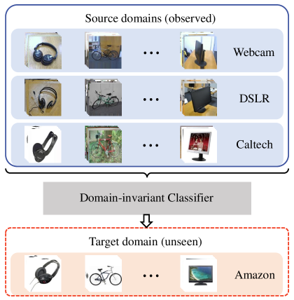
Figure 1: Illustration of DG on Office+Caltech Dataset. One is given source domains: Webcam, DSLR, Caltech, and aims to train a classifier generalizes well on target domain Amazon, which is unavailable in training.

Although various techniques such as kernel methods [Muandet et al., 2013, Ghifary et al., 2017, Li et al., 2018b], support vector machine (SVM) [Khosla et al., 2012, Xu et al., 2014], and deep neural network [Ghifary et al., 2015, Motiian et al., 2017, Li et al., 2017, 2018a, 2018c], have been adopted to solve DG problem, the general idea, which is learning a domain-invariant representation with stable (conditional) distribution in all domains, is shared in most works. Among previous works, kernel-based methods interpret the domain-invariant representation as a feature transformation from the original input space to a transformed space $\mathbb{R}^{q}$, in which the (conditional) distribution shift across domains is minimized.

Unlike previous kernel-based methods, which assume that $\mathbb{P}(Y|X)$ keeps stable and only $\mathbb{P}(X)$ changes across domains (i.e., the covariate shift situation [Shimodaira, 2000]), the problem of DG or domain adaptation has also been investigated from a causal perspective [Zhang et al., 2015]. In particular, Zhang et al. [2013] pointed out that for many learning problems, especially for classification tasks, $Y$ is usually the cause of $X$, and proposed the setting of target shift ($\mathbb{P}(Y)$ changes while $\mathbb{P}(X|Y)$ stays the same across domains), conditional shift ($\mathbb{P}(Y)$ stays the same and $\mathbb{P}(X|Y)$ changes across domains), and their combination accordingly. Gong et al. [2016] proposed to do domain adaptation with conditionally invariant components of $X$, i.e., the transformations of $X$ that have invariant conditional distribution given $Y$ across domains. Li et al. [2018b] then used this idea for DG, under the assumption of conditional shift. Their assumptions stem from the following postulate of causal independence [Janzing and Scholkopf, 2010, Daniušis et al., 2010]:

Postulate 1 (Independence of cause and mechanism).

If $Y$ causes $X$ ($Y\to X$), then the marginal distribution of the cause, $\mathbb{P}(Y)$, and the conditional distribution of the effect given cause, $\mathbb{P}(X|Y)$, are “independent” in the sense that $\mathbb{P}(X|Y)$ contains no information about $\mathbb{P}(Y)$.

According to postulate 1, $\mathbb{P}(X|Y)$ and $\mathbb{P}(Y)$ would behave independently across domains. However, this independence typically does not hold in the anti-causal direction [Schölkopf et al., 2012], so $\mathbb{P}(Y|X)$ and $\mathbb{P}(X)$ tends to vary in a coupled manner across domains. Under assumptions that $\mathbb{P}(X|Y)$ changes while $\mathbb{P}(Y)$ keeps stable, generally speaking, both $\mathbb{P}(Y|X)$ and $\mathbb{P}(X)$ change across domains in the anti-causal direction, which is clearly different from the covariate shift situation.

In this paper, we further relax the causally motivated assumptions in Li et al. [2018b] and propose a novel DG method, which is applicable when both $\mathbb{P}(X|Y)$ and $\mathbb{P}(Y)$ change across domains. Our method focuses on separability between classes and does not enforce the transformed marginal distribution of features to be stable, which allows us to relax the assumption of stable $\mathbb{P}(Y)$. To improve the separability, a novel measure named average class discrepancy, which measures the class discriminative power of source domains, is proposed. Average class discrepancy and other three measures are unified in one objective for feature transformation learning to improve its generalization ability on the target domain. As the second contribution, we derive the bound on excess risk and generalization error for kernel-based domain-invariant feature transformation methods. To the best of our knowledge, this is one of the first works to give theoretical learning guarantees on excess risk of DG. Lastly, experimental results on synthetic and real datasets demonstrate the efficacy of our method in handling varying class prior distributions $\mathbb{P}(Y)$ and complex high-dimensional distributions, respectively.

This paper is organized as follows. Section 2 gives the background on kernel mean embedding. Section 3 introduces our method in detail. Section 4 gives the bounds on excess risk and generalization error for kernel-based methods. Section 5 gives experimental settings and analyzes the results. Section 6 concludes this work.

2 PRELIMINARY ON KERNEL MEAN EMBEDDING

Kernel mean embedding is the main technique to characterize probability distributions in this paper. Kernel mean embedding represents probability distributions as elements in a reproducing kernel Hilbert space (RKHS). More precisely, an RKHS $\mathcal{H}$ over domain $\mathcal{X}$ with a kernel $k$ is a Hilbert space of functions $f:\mathcal{X}\rightarrow\mathbb{R}$. Denoting its inner product by $\langle\cdot,\cdot\rangle_{\mathcal{H}}$, RKHS $\mathcal{H}$ fulfills the reproducing property $\langle f(\cdot),k(\bm{x},\cdot)\rangle_{\mathcal{H}}=f(\bm{x})$, where $\phi(\bm{x})\coloneqq k(\bm{x},\cdot)$ is the canonical feature map of $\bm{x}$. The kernel mean embedding of a distribution $\mathbb{P}(X)$ is defined as [Smola et al., 2007, Gretton et al., 2007]:

$$\mu_{X}\coloneqq\mathbb{E}_{X}[\phi(X)]=\int_{\mathcal{X}}{\phi(\bm{x})d\mathbb{P}(\bm{x})},$$ (1)

where $\mathbb{E}_{X}[\phi(X)]$ is the expectation of $\phi(X)$ with respect to $\mathbb{P}(X)$. It was shown that $\mu_{X}$ is guaranteed to be an element in the RKHS if $\mathbb{E}_{X}[k(\bm{x},\bm{x})]<\infty$ is satisfied [Smola et al., 2007]. In practice, given a finite sample of size $n$, the kernel mean embedding of $\mathbb{P}(X)$ is empirically estimated as $\hat{\mu}_{X}=\frac{1}{n}\sum^{n}_{i=1}\phi(\bm{x}_{i})$, where $\{\bm{x}_{i}\}^{n}_{i=1}$ are independently drawn from $\mathbb{P}(X)$. When $k$ is a characteristic kernel [Schölkopf and Smola, 2001], $\mu_{X}$ captures all information about $\mathbb{P}(X)$ [Sriperumbudur et al., 2008], which means that $\|\mu_{X}-\mu_{X^{\prime}}\|_{\mathcal{H}}=0$ if and only if $\mathbb{P}(X)$ and $\mathbb{P}(X^{\prime})$ are the same distribution.

3 MULTIDOMAIN DISCRIMINANT ANALYSIS

3.1 PROBLEM DEFINITION

DG of classification tasks is studied in this paper. Let $\mathcal{X}$ be the feature space, $\mathcal{Y}$ be the space of class labels, and $c$ be the number of classes. A domain is defined to be a joint distribution $\mathbb{P}(X,Y)$ on $\mathcal{X}\times\mathcal{Y}$. Let $\mathfrak{P}_{\mathcal{X}\times\mathcal{Y}}$ denote the set of domains $\mathbb{P}(X,Y)$ and $\mathfrak{P}_{\mathcal{X}}$ denote the set of distributions $\mathbb{P}(X)$ on $\mathcal{X}$. We assume that there is an underlying finite-variance unimodal distribution over $\mathfrak{P}_{\mathcal{X}\times\mathcal{Y}}$. In practice, domains are not observed directly, but given in the form of finite sample sets.

Assumption 1 (Data-generating process).

Each sample set is assumed to be generated in two separate steps: 1) a domain $\mathbb{P}^{s}(X,Y)$ is sampled from $\mathfrak{P}_{\mathcal{X}\times\mathcal{Y}}$, where $s$ is the domain index; 2) $n^{s}$ independent and identically distributed (i.i.d.) instances are then drawn from $\mathbb{P}^{s}(X,Y)$.

Suppose there are $m$ domains sampled from $\mathfrak{P}_{\mathcal{X}\times\mathcal{Y}}$, the set of $m$ observed sample sets is denoted by $\mathcal{D}=\{\mathcal{D}^{s}\}^{m}_{s=1}$, where each $\mathcal{D}^{s}=\{(\bm{x}^{s}_{i},y^{s}_{i})\}^{n^{s}}_{i=1}$ consists of $n^{s}$ i.i.d. instances from $\mathbb{P}^{s}(X,Y)$. Since in general $\mathbb{P}^{s}(X,Y)\neq\mathbb{P}^{s^{\prime}}(X,Y)$, instances in $\mathcal{D}$ are not i.i.d.

In DG of classification tasks, one aims to incorporate the knowledge in $\mathcal{D}$ into a model which could generalize well on a previously unseen target domain. In this work, features $X$ are first mapped to an RKHS $\mathcal{H}$. Then we resort to learning a transformation from the RKHS $\mathcal{H}$ to a $q$-dimensional transformed space $\mathbb{R}^{q}$, in which instances of the same class are close and instances of different classes are distant from each other. 1-nearest neighbor is adopted to conduct classification in $\mathbb{R}^{q}$.

Table 1: Notations used in the paper

Notation	Description	Notation	Description
$X$, $Y$	feature/label variable	$\bm{x}$, $y$	feature/label instance
$m$, $c$	# domains/classes	$s$, $j$	domain/class index
$\mathfrak{P}_{\mathcal{X}\times\mathcal{Y}}$, $\mathfrak{P}_{\mathcal{X}}$	the set of $\mathbb{P}(X,Y)$ / $\mathbb{P}(X)$	$\mathcal{D}^{s}$	sample set of domain $s$
$\mathbb{P}^{s}_{j}$	class-conditional distribution	$\mu^{s}_{j}$	kernel mean embedding of $\mathbb{P}^{s}_{j}$
$u_{j}$	mean representation of class $j$	$\bar{u}$	mean representation of $\mathcal{D}$
$k$	kernel	$\mathcal{H}_{k}$	RKHS associated with $k$

3.2 REGULARIZATION MEASURES

3.2.1 Average Domain Discrepancy

To achieve the goal that instances of the same class are close to each other, we first consider minimizing the discrepancy of the class-conditional distributions, $\mathbb{P}^{s}(X|Y=j)$, within each class over all source domains.

For ease of notation, the class-conditional distribution of class $j$ in domain $s$, $\mathbb{P}^{s}(X|Y=j)$, is denoted by $\mathbb{P}^{s}_{j}$. Denoting the kernel mean embedding (1) of $\mathbb{P}^{s}_{j}$ by $\mu^{s}_{j}$, the average domain discrepancy is defined below.

Definition 1 (Average domain discrepancy).

Given the set of all class-conditional distributions $\mathcal{P}=\{\mathbb{P}^{s}_{j}\}$ for $s\in\{1,\dots,m\}$ and $j\in\{1,\dots,c\}$, the average domain discrepancy, $\Psi^{\textit{add}}(\mathcal{P})$, is defined as

$$\Psi^{\textit{add}}(\mathcal{P})\coloneqq\frac{1}{c\binom{m}{2}}\sum^{c}_{j=1}\sum_{1\leq s<s^{\prime}\leq m}\|\mu^{s}_{j}-\mu^{s^{\prime}}_{j}\|^{2}_{\mathcal{H}},$$ (2)

where $\binom{m}{2}$ is the number of 2-combinations from a set of $m$ elements, $\|\cdot\|^{2}_{\mathcal{H}}$ denotes the squared norm in RKHS $\mathcal{H}$, and $\|\mu^{s}_{j}-\mu^{s^{\prime}}_{j}\|_{\mathcal{H}}$ is thus the Maximum Mean Discrepancy (MMD; [Gretton et al., 2007]) between $\mathbb{P}^{s}_{j}$ and $\mathbb{P}^{s^{\prime}}_{j}$.

The following theorem shows that $\Psi^{\textit{add}}(\mathcal{P})$ is suitable for measuring the discrepancy between class-conditional distributions of the same class from multiple domains.

Theorem 1.

Let $\mathcal{P}$ denote the set of all class-conditional distributions. If $k$ is a characteristic kernel [Schölkopf and Smola, 2001], $\Psi^{\text{add}}(\mathcal{P})=0$ if and only if $\mathbb{P}^{1}_{j}=\mathbb{P}^{2}_{j}=\dots=\mathbb{P}^{m}_{j}$, for $j=1,\dots,c$.

Proof.

Since $k$ is a characteristic kernel, $\|\mu_{\mathbb{P}}-\mu_{\mathbb{Q}}\|_{\mathcal{H}}$ is a metric and attains 0 if and only if $\mathbb{P}=\mathbb{Q}$ for any distributions $\mathbb{P}$ and $\mathbb{Q}$ [Sriperumbudur et al., 2008]. Therefore, $\|\mu^{s}_{j}-\mu^{s^{\prime}}_{j}\|_{\mathcal{H}}=0$ if and only if $\mathbb{P}^{s}_{j}=\mathbb{P}^{s^{\prime}}_{j}$ for all $s$ and $s^{\prime}$ given $j$, which means $\mathbb{P}^{1}_{j}=\mathbb{P}^{2}_{j}=\dots=\mathbb{P}^{m}_{j}$ within each class $j$. Conversely, if $\mathbb{P}^{1}_{j}=\mathbb{P}^{2}_{j}=\dots=\mathbb{P}^{m}_{j}$ for $j=1,\dots,c$, then each term $\|\mu^{s}_{j}-\mu^{s^{\prime}}_{j}\|=0$ and $\Psi^{\text{add}}(\mathcal{P})$ is thus 0. ∎

3.2.2 Average Class Discrepancy

Minimizing average domain discrepancy $\Psi^{\textit{add}}$ (2) would make the means of class-conditional distributions of the same class close in $\mathcal{H}$. However, it is possible that the means of class-conditional distributions of different classes are also close, which is a major source of performance reduction of existing kernel-based DG methods. To this end, average class discrepancy is proposed.

Definition 2 (Average class discrepancy).

Let $\mathcal{P}$ denote the set of all class-conditional distributions. The average class discrepancy is defined as

$$\Psi^{\textit{acd}}(\mathcal{P})\coloneqq\frac{1}{\binom{c}{2}}\sum_{1\leq j<j^{\prime}\leq c}\|u_{j}-u_{j^{\prime}}\|^{2}_{\mathcal{H}},$$ (3)

where $u_{j}=\sum^{m}_{s=1}\mathbb{P}(S=s|Y=j)\mu^{s}_{j}$ is the mean representation of class $j$ in RKHS $\mathcal{H}$.

It was shown in Sriperumbudur et al. [2010] that the MMD between two distributions $\mathbb{P}$ and $\mathbb{Q}$, $\text{MMD}[\mathbb{P},\mathbb{Q}]\leq\sqrt{C}W_{1}(\mathbb{P},\mathbb{Q})$ for some constant $C$ satisfying $\sup_{\bm{x}\in\mathcal{X}}k(\bm{x},\bm{x})\leq C<\infty$, where $W_{1}(\mathbb{P},\mathbb{Q})$ denotes the first Wasserstein distance [Barrio et al., 1999] between distributions $\mathbb{P}$ and $\mathbb{Q}$. In other words, if $\mathbb{P}$ and $\mathbb{Q}$ are distant in MMD metric, they are also distant in the first Wasserstein distance. Therefore, distributions of different classes tend to be distinguishable by maximizing average class discrepancy, $\Psi^{\textit{acd}}(\mathcal{P})$.

3.2.3 Incorporating Instance-level Information

Both average domain discrepancy $\Psi^{\textit{add}}(\mathcal{P})$ (2) and average class discrepancy $\Psi^{\textit{acd}}(\mathcal{P})$ (3) are defined based on the kernel mean embedding of class-conditional distributions $\mathbb{P}^{s}_{j}$. By simultaneously minimizing $\Psi^{\textit{add}}$ (2) and maximizing $\Psi^{\textit{acd}}$ (3), one would make class-conditional kernel mean embeddings within each class close and the those of different classes distant in $\mathcal{H}$. However, certain subtle information, such as the compactness of the distribution, is not captured in $\Psi^{\textit{add}}$ and $\Psi^{\textit{acd}}$. As a result, although all mean embeddings satisfy the desired condition, there may still be a high chance of misclassification for some instances. To incorporate such information conveyed in each instance, we propose two extra measures based on kernel Fisher discriminant analysis [Mika et al., 1999]. The first is multidomain between-class scatter.

Definition 3 (Multidomain between-class scatter).

Let $\mathcal{D}$ denote the set of $n$ instances from $m$ domains, each of which consists of $c$ classes. The multidomain between-class scatter is

$$\Psi^{\textit{mbs}}(\mathcal{D})\coloneqq\frac{1}{n}\sum^{c}_{j=1}n_{j}\|u_{j}-\bar{u}\|^{2}_{\mathcal{H}},$$ (4)

where $n_{j}$ is the total number of instances in class $j$, and $\bar{u}=\sum^{c}_{j=1}P(Y=j)u_{j}$ is the the mean representation of the entire set $\mathcal{D}$ in $\mathcal{H}$.

Both $\Psi^{\textit{mbs}}(\mathcal{D})$ and $\Psi^{\textit{acd}}(\mathcal{P})$ measure the discrepancy between the distributions of different classes. The difference stems from the weight $n_{j}$ in $\Psi^{\textit{mbs}}(\mathcal{D})$ (4). By adding $n_{j}$, each term in $\Psi^{\textit{mbs}}(\mathcal{D})$ is equivalent to pooling all instances of the same class together and summing up their distance to $\bar{u}$. In other words, $\Psi^{\textit{mbs}}(\mathcal{D})$ corresponds to a simple pooling scheme. Note that when the proportion of instances of each class is the same across all domains (i.e., $n^{s}_{j}/n^{s}=n^{s^{\prime}}_{j}/n^{s^{\prime}},\forall s,s^{\prime}$ for $j=1,\dots,c$, where $n^{s}_{j}$ is the number of instances of class $j$ in domain $s$), $\Psi^{\textit{mbs}}(\mathcal{D})$ is consistent with the between-class scatter in Mika et al. [1999].

Multidomain within-class scatter, as a straightforward counterpart of multidomain between-class scatter (4), is defined as follows.

Definition 4 (Multidomain within-class scatter).

Let $\mathcal{D}$ denote the set of $n$ instances from $m$ domains, each of which consists of $c$ classes. The multidomain within-class scatter is

$$\Psi^{\textit{mws}}(\mathcal{D})\coloneqq\frac{1}{n}\sum^{c}_{j=1}\sum^{m}_{s=1}\sum^{n^{s}_{j}}_{i=1}\|\phi(\bm{x}^{s}_{i\in j})-u_{j}\|^{2}_{\mathcal{H}},$$ (5)

where $\bm{x}^{s}_{i\in j}$ denotes the feature vector of $i$th instance of class $j$ in domain $s$.

The definition above indicates that multidomain within-class scatter measures the sum of the distance between the canonical feature map of each instance and the mean representation in RKHS $\mathcal{H}$ of the class it belongs to. It differs from average domain discrepancy in that the information of every instance is considered in multidomain within-class scatter. As a result, by minimizing $\Psi^{\textit{mws}}(\mathcal{D})$, one increases the overall compactness of the distributions across classes. Similar to $\Psi^{\textit{mbs}}(\mathcal{D})$, when the proportion of instances of each class is the same across all domains (i.e., $n^{s}_{j}/n^{s}=n^{s^{\prime}}_{j}/n^{s^{\prime}},\forall s,s^{\prime}$ for $j=1,\dots,c$), $\Psi^{\textit{mws}}(\mathcal{D})$ is consistent with the within-class scatter in Mika et al. [1999].

We note that each of the measures has its unique contribution and that ignoring any of them may lead to sub-optimal solutions, as demonstrated by the empirical results and illustrated in Appendix A.

3.3 FEATURE TRANSFORMATION

Our method resorts to finding a suitable transformation from RKHS $\mathcal{H}$ to a $q$-dimensional transformed space $\mathbb{R}^{q}$, i.e., $\mathbf{W}:\mathcal{H}\mapsto\mathbb{R}^{q}$. We elaborate how the proposed measures are transformed to $\mathbb{R}^{q}$ in this section.

According to the property of norm in RKHS, $\Psi^{\textit{add}}(\mathcal{P})$ can be equivalently computed as

$$\operatorname{tr}\left(\frac{1}{c\binom{m}{2}}\sum^{c}_{j=1}\sum_{1\leq s<s^{\prime}\leq m}(\mu^{s}_{j}-\mu^{s^{\prime}}_{j})(\mu^{s}_{j}-\mu^{s^{\prime}}_{j})^{T}\right),$$ (6)

where $\operatorname{tr}(\cdot)$ denotes the trace operator.

Let the data matrix $\mathbf{X}=\left[\bm{x}_{1},\dots,\bm{x}_{n}\right]^{T}\in\mathbb{R}^{n\times d}$, where $d$ is the dimension of input features $X$ and $n=\sum^{m}_{s=1}n^{s}$, and the feature matrix $\bm{\Phi}=\left[\phi(\bm{x}_{1}),\dots,\phi(\bm{x}_{n})\right]^{T}$, where $\phi:\mathbb{R}^{d}\mapsto\mathcal{H}$ denotes the canonical feature map. Then $\mathbf{W}$ can be expressed as a linear combination of all canonical feature maps in $\bm{\Phi}$ [Schölkopf et al., 1998], i.e., $\mathbf{W}=\bm{\Phi}^{T}\mathbf{B}$, where $\mathbf{B}$ is a matrix collecting coefficients of canonical feature maps. Then by applying the transformation $\mathbf{W}$, $\Psi^{\textit{add}}(\mathcal{P})$ in trace formulation (6) becomes

$$\Psi^{\textit{add}}_{\mathbf{B}}=\operatorname{tr}\left(\mathbf{B}^{T}\mathbf{GB}\right),$$ (7)

where

$$\mathbf{G}=\frac{1}{c\binom{m}{2}}\sum^{c}_{j=1}\sum_{1\leq s<s^{\prime}\leq m}\bm{\Phi}(\mu^{s}_{j}-\mu^{s^{\prime}}_{j})(\mu^{s}_{j}-\mu^{s^{\prime}}_{j})^{T}\bm{\Phi}^{T}.$$ (8)

Similarly, after applying the transformation $\mathbf{W}$, average class discrepancy $\Psi^{\textit{acd}}(\mathcal{P})$ (3), multidomain between-class scatter $\Psi^{\textit{mbs}}(\mathcal{D})$ (4), and multidomain within-class scatter $\Psi^{\textit{mws}}(\mathcal{D})$ (5) are given by:

$$\Psi^{\textit{acd}}_{\mathbf{B}}=\operatorname{tr}\left(\mathbf{B}^{T}\mathbf{FB}\right),\Psi^{\textit{mbs}}_{\mathbf{B}}=\operatorname{tr}\left(\mathbf{B}^{T}\mathbf{PB}\right),$$

$$\Psi^{\textit{mws}}_{\mathbf{B}}=\operatorname{tr}\left(\mathbf{B}^{T}\mathbf{QB}\right),$$ (9)

where

$$\mathbf{F}=\frac{1}{\binom{c}{2}}\sum_{1\leq j<j^{\prime}\leq c}\bm{\Phi}(u_{j}-u_{j^{\prime}})(u_{j}-u_{j^{\prime}})^{T}\bm{\Phi}^{T},$$ (10)

$$\mathbf{P}=\frac{1}{n}\sum^{c}_{j=1}n_{j}\bm{\Phi}(u_{j}-\bar{u})(u_{j}-\bar{u})^{T}\bm{\Phi}^{T},$$ (11)

$$\mathbf{Q}=\frac{1}{n}\sum^{c}_{j=1}\sum^{m}_{s=1}\sum^{n^{s}_{j}}_{i=1}\bm{\Phi}(\phi(\bm{x}^{s}_{i\in j})-u_{j})(\phi(\bm{x}^{s}_{i\in j})-u_{j})^{T}\bm{\Phi}^{T}.$$ (12)

3.4 EMPIRICAL ESTIMATION

In practice, one exploits a finite number of instances from $m$ source domains to estimate the transformed measures in $\mathbb{R}^{q}$. Since all measures depend on $\mu^{s}_{j}$ and $u_{j}$, the estimation of measures reduces to the estimation of $\mu^{s}_{j}$ and $u_{j}$ ($s=1,\dots,m,j=1,\dots,c$) using the source data. Let $\bm{x}^{s}_{i\in j}$ denote the feature vector of $i$th instance of class $j$ in domain $s$ and $n^{s}_{j}$ denote the total number of instances of class $j$ in domain $s$, each $\mu^{s}_{j}$ can be empirically estimated as

$$\hat{\mu}^{s}_{j} =\frac{1}{n^{s}_{j}}\sum^{n^{s}_{j}}_{i=1}\phi(\bm{x}^{s}_{i\in j}).$$ (13)

The empirical estimation of $u_{j}$ requires $\mathbb{P}(S=s|Y=j)$, which can be estimated using Bayes rule as $\mathbb{P}(S=s|Y=j)=\frac{\text{Pr}(Y=j|S=s)\text{Pr}(S=s)}{\text{Pr}(Y=j)}$. Since it is usually hard to model the underlying distribution over $\mathfrak{P}_{\mathcal{X}\times\mathcal{Y}}$, we assume that the probabilities of sampling all source domains are equal, i.e., $\text{Pr}(S=s)=\frac{1}{m}$ for $s=1,\dots,m$ given $\mathcal{D}$. As a result, $\mathbb{P}(S=s|Y=j)=\frac{n^{s}_{j}/n^{s}}{\sum^{m}_{s^{\prime}=1}(n^{s^{\prime}}_{j}/n^{s^{\prime}})}$. Then the empirical estimation of the mean representation of class $j$ in RKHS $\mathcal{H}$ is given by

$$\hat{u}_{j} =\sum^{m}_{s=1}\frac{n^{s}_{j}/n^{s}}{\sum^{m}_{s^{\prime}=1}(n^{s^{\prime}}_{j}/n^{s^{\prime}})}\hat{\mu}^{s}_{j}.$$ (14)

By substituting the empirical class-conditional kernel mean embedding (13) and empirical mean representation of each class (14) into formulation (8), (10), (11), and (12), these matrices can be estimated from $m$ observed sample sets using the kernel trick [Theodoridis and Koutroumbas, 2008].

3.5 THE OPTIMIZATION PROBLEM

Following the solution in Ghifary et al. [2017] and in the spirit of Fisher’s discriminant analysis [Mika et al., 1999], we unify measures introduced in previous sections and solve the matrix $\mathbf{B}$ as

$$\operatorname*{arg\,max}_{\mathbf{B}}\frac{\Psi^{\textit{acd}}_{\mathbf{B}}+\Psi^{\textit{mbs}}_{\mathbf{B}}}{\Psi^{\textit{add}}_{\mathbf{B}}+\Psi^{\textit{mws}}_{\mathbf{B}}}.$$ (15)

It can be seen that through maximizing the numerator, the objective (15) preserves the separability among different classes. Through minimizing the denominator, (15) tries to find a domain-invariant transformation which improves the overall compactness of distributions of all classes and make the class-conditional distributions of the same class as close as possible.

By substituting the transformed average domain discrepancy (7), average class discrepancy, multidomain between-class scatter, and multidomain within-class scatter (9), adding $\mathbf{W}^{T}\mathbf{W}=\mathbf{B}^{T}\mathbf{KB}$ for regularization, and introducing a trade-off between the measures for further flexibility into the objective (15), we aim to achieve

$$\operatorname*{arg\,max}_{\mathbf{B}}=\frac{\operatorname{tr}\left(\mathbf{B}^{T}\left(\beta\mathbf{F}+(1-\beta)\mathbf{P}\right)\mathbf{B}\right)}{\operatorname{tr}\left(\mathbf{B}^{T}(\gamma\mathbf{G}+\alpha\mathbf{Q}+\mathbf{K})\mathbf{B}\right)},$$ (16)

where $\alpha$, $\beta$, and $\gamma$ are trade-off parameters controlling the significance of corresponding measures. Since the objective (16) is invariant to re-scaling of $\mathbf{B}$, rewriting (16) as a constrained optimization problem and setting the derivative of its Lagrangian to zero (see Appendix B) yields the following generalized eigenvalue problem:

$$\left(\beta\mathbf{F}+(1-\beta)\mathbf{P}\right)\mathbf{B}=\left(\gamma\mathbf{G}+\alpha\mathbf{Q}+\mathbf{K}\right)\mathbf{B}\bm{\Gamma},$$ (17)

where $\bm{\Gamma}=\text{diag}(\lambda_{1},\dots,\lambda_{q})$ is the diagonal matrix collecting $q$ leading eigenvalues, $\mathbf{B}$ is the matrix collecting corresponding eigenvectors.

Computing the matrices $\mathbf{G}$, $\mathbf{F}$, $\mathbf{P}$, and $\mathbf{Q}$ takes $\mathcal{O}(n^{2})$. Solving the generalized eigenvalue problem (17) takes $\mathcal{O}(qn^{2})$. In sum, the overall computational complexity is $\mathcal{O}(n^{2}+qn^{2})$, which is the same as existing kernel-based methods. After the transformation learning, unseen target instances can then be transformed into $\mathbb{R}^{q}$ using $\mathbf{B}$ and $\bm{\Gamma}$. We term the proposed method Multidomain Discriminant Analysis (MDA) and summarize the algorithm in Algorithm 1.

input : $\mathcal{D}=\{\mathcal{D}^{s}\}_{s=1}^{m}$ - the set of instances from $m$ domains;

$\alpha$, $\beta$, $\gamma$ - trade-off parameters.

output : Optimal projection $\mathbf{B}_{n\times q}$;

corresponding eigenvalues $\bm{\Gamma}$.

Construct kernel matrix $\mathbf{K}$ from $\mathcal{D}$, whose entry on $i$th row and $i^{\prime}$th column $[\mathbf{K}]_{ii^{\prime}}=k(\bm{x}_{i},\bm{x}_{i^{\prime}})$;

Compute matrices $\mathbf{G}$, $\mathbf{F}$, $\mathbf{P}$, $\mathbf{Q}$ from (8), (10), (11), (12), respectively;

Center the kernel matrix as $\mathbf{K}\leftarrow\mathbf{K}-\mathbf{1}_{n}\mathbf{K}-\mathbf{K}\mathbf{1}_{n}$ $+\mathbf{1}_{n}\mathbf{K}\mathbf{1}_{n}$, where $\mathbf{1}_{n}\in\mathbb{R}^{n\times n}$ denotes a matrix with all entries equal to $\frac{1}{n}$;

Solve (17) for the projection $\mathbf{B}$ and corresponding eigenvalues $\bm{\Gamma}$, then select $q$ leading components. Target domain transformation 

Denote the set of instances from the target domain by $\mathcal{D}^{t}$, one first constructs the kernel matrix $\mathbf{K}^{t}$, where $[\mathbf{K}^{t}]_{i^{\prime}i}=k(\bm{x}^{t}_{i^{\prime}},\bm{x}_{i})$, $\forall\bm{x}^{t}_{i^{\prime}}\in\mathcal{D}^{t}$, $\forall\bm{x}_{i}\in\mathcal{D}$;

Center the kernel matrix as $\mathbf{K}^{t}\leftarrow\mathbf{K}^{t}-\mathbf{1}_{n^{t}}\mathbf{K}^{t}-$ $\mathbf{K}^{t}\mathbf{1}_{n}+\mathbf{1}_{n^{t}}\mathbf{K}^{t}\mathbf{1}_{n}$, where $n^{t}$ is the number of instances in $\mathcal{D}^{t}$;

Then the transformed features of the target domain are given by $\mathbf{X}^{t}=\mathbf{K}^{t}\mathbf{B}\bm{\Gamma}^{-\frac{1}{2}}$.

Algorithm 1 Multidomain discriminant analysis

4 LEARNING THEORY ANALYSIS

We analyze the the excess risk and generalization error bound after applying feature transformation $\mathbf{W}$.

In standard setting of learning theory analysis, the decision functions of interest are $f:\mathcal{X}\mapsto\mathcal{Y}$. However, our DG problem setting is much more general in the sense that not only $\mathbb{P}(X)$ changes (as in the covariate shift setting), but $\mathbb{P}(Y|X)$, which corresponds to $f$ in learning theory, also changes across domains. As a result, the decision functions of interest in our analysis are $f:\mathfrak{P}_{\mathcal{X}}\times\mathcal{X}\mapsto\mathcal{Y}$. $\mathbb{P}^{s}$ and $\mathbb{P}^{s}_{X}$ are used interchangeably to denote the marginal distribution of $X$ in domain $s$.

Let $\bar{k}$ be a kernel on $\mathfrak{P}_{\mathcal{X}}\times\mathcal{X}$ and $\mathcal{H}_{\bar{k}}$ be the associated RKHS. As in Blanchard et al. [2011], we consider kernel $\bar{k}=k_{\mathbb{P}}(\mathbb{P}^{1},\mathbb{P}^{2})k_{x}(x_{1},x_{2})$, where $k_{\mathbb{P}}$ and $k_{x}$ are kernels on $\mathfrak{P}_{\mathcal{X}}$ and $\mathcal{X}$, respectively. To ensure that $\bar{k}$ is universal, we consider a particular form for $k_{\mathbb{P}}$. Let $k^{\prime}_{x}$ be another kernel on $\mathcal{X}$ and $\mathcal{H}_{k^{\prime}_{x}}$ be its associated RKHS, $\gamma$ be a mapping $\gamma:\mathfrak{P}_{\mathcal{X}}\mapsto\mathcal{H}_{k^{\prime}_{x}}$. Then $k_{\mathbb{P}}$ defined as a kernel $k_{\gamma}$ on $\mathcal{H}_{k^{\prime}_{x}}$, i.e. $k_{\mathbb{P}}(\mathbb{P}^{1},\mathbb{P}^{2})=k_{\gamma}(\gamma(\mathbb{P}^{1}),\gamma(\mathbb{P}^{2}))$ would lead $\bar{k}$ to be universal [Blanchard et al., 2011]. We consider following assumptions regarding the kernels and loss function in our analysis:

Assumption 2.

The kernels $k_{x}$, $k^{\prime}_{x}$ and $k_{\gamma}$ are bounded respectively by $U^{2}_{k_{x}}$, $U^{2}_{k^{\prime}_{x}}$ and $U^{2}_{k_{\gamma}}$.

Assumption 3.

The canonical feature map $\gamma_{k_{\gamma}}:\mathcal{H}_{k^{\prime}_{x}}\mapsto\mathcal{H}_{k_{\gamma}}$, where $\mathcal{H}_{k_{\gamma}}$ is the RKHS associated with $k_{\gamma}$, fulfills that $\forall v,w\in\mathcal{H}_{k^{\prime}_{X}}$, there is a constant $L_{k_{\gamma}}$ satisfying

$$\|\gamma_{k_{\gamma}}(v)-\gamma_{k_{\gamma}}(w)\|\leq L_{k_{\gamma}}\|v-w\|.$$

Assumption 4.

The loss function $\ell:\mathbb{R}\times\mathcal{Y}\mapsto\mathbb{R}_{+}$ is $L_{\ell}$-Lipschitz in its first variable and bounded by $U_{\ell}$.

Assumption 2 and 3 are satisfied when the kernels are bounded. An example of widely adopted bounded kernel is the Gaussian kernel. As a result, we also adopt Gaussian kernel throughout our algorithm.

Let $\tilde{X}^{t}=(\mathbb{P}^{t}_{X},X^{t})$ and $Y^{t}$ denote the extended input and output pattern of decision function $f$ over target domain, respectively. The quantity of interest is the excess risk, which is the difference between expected test loss of empirical loss minimizer and expected loss minimizer. For functions in the unit ball centered at the origin in the RKHS of $\phi(\tilde{X}^{t})$, the control of the excess risk is given in the following theorem.

Theorem 2.

Under assumptions 2 – 4, and further assuming that $\|\hat{f}\|_{\mathcal{H}_{\bar{k}}}\leq 1$ and $\|f^{*}\|_{\mathcal{H}_{\bar{k}}}\leq 1$, where $\hat{f}$ denotes the empirical risk minimizer and $f^{*}$ denotes the expected risk minimizer, then with probability at least $1-\delta$ there is

$$\mathbb{E}[\ell(\hat{f}(\tilde{X^{t}}\mathbf{W}),Y^{t})]-\mathbb{E}[\ell(f^{*}(\tilde{X^{t}}\mathbf{W}),Y^{t})]$$

$$\leq \ 4L_{\ell}L_{k_{\gamma}}U_{k^{\prime}_{x}}U_{k_{x}}\sqrt{\frac{\operatorname{tr}(\mathbf{B}^{T}\mathbf{KB})}{n}}+\sqrt{\frac{2\log 2\delta^{-1}}{n}},$$ (18)

where the expectations are taken over the joint distribution of the test domain $\mathbb{P}^{t}(X^{t},Y^{t})$, $n$ is the number of training samples, and $\mathbf{K}=\bm{\Phi}\bm{\Phi}^{T}$.

See Appendix C for proof. The first term in the bound above involves the size of the distortion $\operatorname{tr}(\mathbf{B}^{T}\mathbf{KB})$ introduced by $\mathbf{B}$. Therefore, a poor choice of $\mathbf{B}$ would loose the guarantee. The second term is of order $O(n^{-1/2})$ so it would converge to zero as $n$ tends to infinity given $\delta$.

Another quantity of interest is the generalization error bound, which is the difference between the expected test loss and empirical training loss of the empirical loss minimizer. The generalization error bound of DG in a general setting is given in Blanchard et al. [2011]. Therefore, we derive it for the case where one applies feature transformation involving $\mathbf{B}$. Let $\hat{\tilde{X}}^{s}_{i}$ denote the input pattern $(\hat{\mathbb{P}}^{s},x^{s}_{i})$, where $\hat{\mathbb{P}}^{s}$ is the empirical distribution over features in domain $s$, and $x^{s}_{i}$ is the $i$th observed feature in domain $s$. Similarly, $y^{s}_{i}$ is the $i$th label in domain $s$. With $\mathcal{E}(f,\infty)$ being the expected test loss, the generalization bound involving $\mathbf{B}$ is given in the following theorem.

Table 2: Generating Distributions of Synthetic Data

Domain	Domain 1			Domain 2			Domain 3
Class	1	2	3	1	2	3	1	2	3
$X_{1}$	(1, 0.3)	(2, 0.3)	(3, 0.3)	(3.5, 0.3)	(4.5, 0.3)	(5.5, 0.3)	(8, 0.3)	(9.5, 0.3)	(10, 0.3)
$X_{2}$	(2, 0.3)	(1, 0.3)	(2, 0.3)	(2.5, 0.3)	(1.5, 0.3)	(2.5, 0.3)	(2.5, 0.3)	(1.5, 0.3)	(2.5, 0.3)
# instances	50	50	50	50	50	50	50	50	50

Theorem 3.

Under assumptions 2 – 4, and assuming that all source sample sets are of the same size, i.e. $n^{s}=\bar{n}$ for $s=1,\dots,m$, then with probability at least $1-\delta$ there is

$$\sup_{\|f\|_{\mathcal{H}_{\bar{k}}}\leq 1}\left|\frac{1}{m}\sum^{m}_{s=1}\frac{1}{n^{s}}\sum^{n^{s}}_{i=1}\ell\left(f(\hat{\tilde{X}}^{s}_{i}\mathbf{W}),y^{s}_{i}\right)-\mathcal{E}(f,\infty)\right|$$

$$\leq U_{\ell}\left(\sqrt{\frac{\log 2\delta^{-1}}{2m\bar{n}}}+\sqrt{\frac{\log\delta^{-1}}{2m}}\right)+\sqrt{\operatorname{tr}(\mathbf{B}^{T}\mathbf{KB})}$$

$$\ \left(c_{1}\sqrt{\frac{\log 2\delta^{-1}m}{\bar{n}}}+c_{2}\left(\sqrt{\frac{1}{m\bar{n}}}+\sqrt{\frac{1}{m}}\right)\right),$$ (19)

where $c_{1}=2\sqrt{2}L_{\ell}U_{k_{x}}L_{k_{\gamma}}U_{k^{\prime}_{x}}$, $c_{2}=2L_{\ell}U_{k_{x}}U_{k_{\gamma}}$.

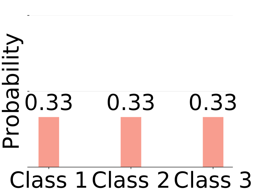
(a)

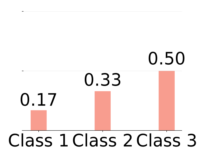
(b)

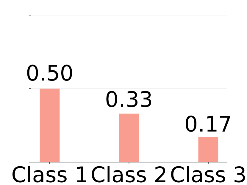
(c)

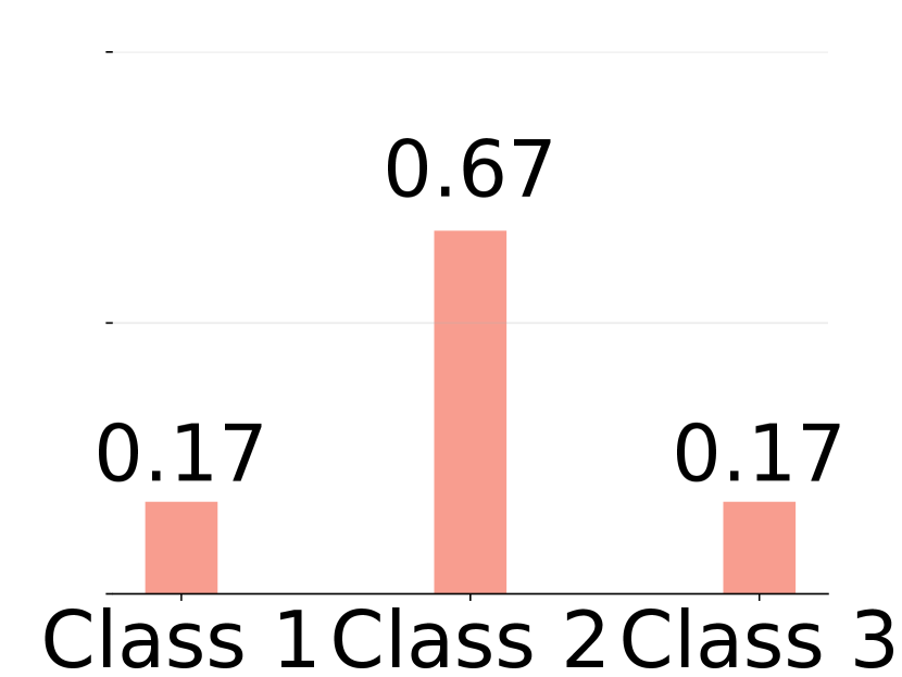
(d)

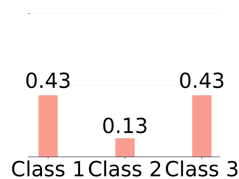
(e)

Figure 2: Class Prior Distributions $\mathbb{P}(Y)$ in Synthetic Experiments.

Table 3: Accuracy (%) of Synthetic Experiments (bold italic and bold indicate the best and second best).

$\mathbb{P}^{1}(Y)$	2(a)	2(b)	2(c)	2(d)	2(e)	2(a)	2(a)	2(a)	2(a)
$\mathbb{P}^{2}(Y)$	2(a)	2(a)	2(a)	2(a)	2(a)	2(b)	2(c)	2(d)	2(e)
SVM	56.00	34.00	33.33	33.33	33.33	33.33	40.00	36.00	60.00
KPCA	66.00	62.00	66.67	33.33	33.33	65.33	36.00	40.00	14.00
KFD	78.67	38.67	46.00	74.67	47.33	49.33	34.00	19.33	76.00
L-SVM	56.00	60.00	64.00	62.00	60.67	64.67	45.33	46.00	59.33
DICA	93.33	84.67	76.00	84.00	84.67	54.00	95.33	71.33	88.67
SCA	79.33	72.00	84.67	57.33	76.00	59.33	84.67	61.33	81.33
CIDG	90.67	87.33	74.67	77.33	86.67	83.33	92.00	82.00	86.00
MDA	96.67	96.00	97.33	94.00	94.00	91.33	95.33	94.00	94.00

See Appendix D for proof. The first term is of order $O(m^{-1/2})$ and converges to zero as $m\rightarrow\infty$. The second term, involving $\operatorname{tr}(\mathbf{B}^{T}\mathbf{KB})$, again depends on the choice of $\mathbf{B}$. The remaining part would converge to zero only if both $m$ and $\bar{n}$ tend to infinity and $\log m/\bar{n}=o(1)$. In a general perspective, our method, as well as existing ones relying on feature extraction can all be viewed as ways of finding transformation $\mathbf{B}$, which could minimize the generalization bound on the test domain, under different understandings of the DG problem.

5 EXPERIMENTS

5.1 EXPERIMENTAL CONFIGURATION

We compare MDA with the following 9 methods:

• Baselines: 1-nearest neighbor (1NN) and support vector machine (SVM) with RBF kernel.

• Feature extraction methods: kernel principal component analysis (KPCA; [Schölkopf et al., 1998]) and kernel Fisher discriminant analysis (KFD; [Mika et al., 1999]). 1NN is applied on the transformed features for classification.

• SVM-based DG method: low-rank exemplar-SVMs (L-SVM; [Xu et al., 2014]).

• Neural network-based DG method: CCSA [Motiian et al., 2017]. The network setting follows [Motiian et al., 2017].

• Kernel-based DG methods: domain invariant component analysis (DICA; [Muandet et al., 2013]), scatter component analysis (SCA; [Ghifary et al., 2017]), and conditional invariant DG (CIDG; [Li et al., 2018b]). 1NN is applied on the domain-invariant representations for classification.

For 1NN and SVM baselines, instances in source domains are directly combined for training in both synthetic and real data experiments. For other methods, in experiments with synthetic data, the models are trained on two source sample sets, validated on one target sample set, and tested on the other target sample set. In real data experiments, we first selected hyper-parameters by 5-fold cross-validation using only labeled source sample sets. Then the model with optimal parameter settings was applied on the target domain. The classification accuracy on the target domain serves as the evaluation criterion for different methods. Since measures in section 3.2 are defined as the averaged distance, we naturally put them on a equal footing by setting $\beta=0.5$, $\alpha=\gamma=1$. Thus in practice, these parameters are set to be an interval containing values in the above balanced case. The hyper-parameters required by each method and the values validated in the experiments are given in Appendix E.

Table 4: Accuracy (%) of Office+Caltech Dataset

Target	A	C	A, C	W, D	W, C	D, C
1NN	89.80	84.16	78.63	80.60	86.29	85.28
SVM	91.96	85.75	77.66	84.51	87.31	86.72
KPCA	89.87	83.35	66.46	79.65	85.83	84.45
KFD	91.75	85.66	74.68	82.96	87.59	86.64
L-SVM	91.64	85.39	80.55	83.33	88.09	87.10
CCSA	90.98	83.37	77.56	80.04	85.80	84.91
DICA	92.59	83.17	63.67	83.85	87.59	86.25
SCA	91.96	83.35	73.04	83.85	87.31	86.25
CIDG	92.38	81.39	69.87	82.74	87.45	85.63
MDA	93.47	86.89	82.56	84.89	88.91	88.23

Table 5: Accuracy (%) of VLCS Dataset

Target	V	L	C	S	V, L	V, C	V, S	L, C	L, S	C, S
1NN	60.19	53.57	89.94	55.74	57.26	58.54	50.59	66.06	58.13	66.25
SVM	68.57	59.26	93.99	65.27	61.80	64.39	55.89	70.08	64.10	71.09
KPCA	60.69	54.86	83.89	55.61	57.54	57.50	49.46	67.48	56.05	66.15
KFD	61.64	60.54	86.78	58.75	57.33	46.84	53.20	70.03	61.64	67.87
L-SVM	58.14	39.87	75.56	52.92	52.25	56.64	48.27	61.24	56.65	66.27
CCSA	60.39	58.80	86.88	59.87	59.27	55.02	51.56	69.94	61.41	68.49
DICA	62.71	59.38	86.15	57.28	58.11	55.08	55.17	70.01	61.44	70.30
SCA	62.13	58.24	88.48	60.66	60.66	57.59	54.66	71.90	61.57	70.71
CIDG	64.16	57.91	90.11	59.48	60.54	54.56	55.77	70.74	62.48	69.83
MDA	66.86	61.78	92.64	59.58	59.60	63.72	55.98	72.88	62.83	72.00

5.2 SYNTHETIC DATA

We investigate the influence of variation in the class prior distribution, $\mathbb{P}(Y)$, on different DG methods. Two-dimensional data is generated from three different domains and each domain consists of three classes. Each dimension of the data follows a Gaussian distribution $\mathcal{N}(\mu,\sigma)$, where $\mu$ is the mean and $\sigma$ is the standard deviation. The settings of the distribution of the synthetic data are listed in Table 2. Domains 1 and 2 are source domains and domain 3 is the target domain. The setting in Table 2 is the base condition where class prior distributions are uniform in all domains, i.e., $\mathbb{P}^{1}(Y)=\mathbb{P}^{2}(Y)=\mathbb{P}^{3}(Y)$. Then we change $\mathbb{P}(Y)$ of one source domain to be distributions shown in Figure 2(b) to 2(e) and keep $\mathbb{P}(Y)$ of the other source domain and target domain uniform to compare different DG methods. Note that CCSA is based on convolutional neural network and thus not suitable for 2-dimensional synthetic data.

The results of different methods on different settings of class prior distributions in source domains are given in Table 3 (also visualized in Appendix F). The accuracy of 1NN is 33.33% in all cases thus omitted in Table 3. It can be seen that MDA performs best in the base setting, as well as all settings with different $\mathbb{P}(Y)$ in source domains. DICA performs equally well as MDA in (2a, 2c) setting but its accuracy is heavily influenced by the variation in $\mathbb{P}(Y)$. Compared with other methods, MDA is much more robust against the variation in $\mathbb{P}(Y)$, which is consistent with our expectation because we essentially work with the class-conditional, not the marginal, distributions.

5.3 OFFICE+CALTECH DATASET

We evaluate the performance of different DG methods on Office+Caltech dataset [Gong et al., 2012], which is a widely used benchmark for DG tasks. Office+Caltech consists of photos from four different datasets: Amazon (A), Webcam (W), DSLR (D), and Caltech-256 (C) [Griffin et al., 2007]. Since there are 10 shared classes in these datasets, photos of these classes are selected and those from the same original dataset form one domain in Office+Caltech. Thus, the domains within Office+Caltech corresponds to the biases of different data collection procedures [Torralba and Efros, 2011]. The 4096-dimensional $\text{DeCAF}_{6}$ features [Donahue et al., 2014] are adopted in the experiments to ensure that the feature spaces, $\mathcal{X}$, are consistent across all domains.

The accuracies on different choices of target domains are shown in Table 4. MDA again performs best, yet by a smaller margin of improvement compared to that of the synthetic experiment. In particular, MDA is the only kernel-based method that outperforms 1NN in ($A$, $C$) case which is probably because of the newly proposed average class discrepancy (3). L-SVM outperforms other kernel-based methods and ranks the second. Note that other 4 cases, such as A, D, C $\to$ W, are not reported since 1NN baseline could already achieve accuracies higher than $90\%$.

5.4 VLCS DATASET

The second real data experiment uses the VLCS dataset. It consists of photos of five common classes extracted from four datasets: Pascal VOC2007 (V) [Everingham et al., 2010], LabelMe (L) [Russell et al., 2008], Caltech-101 (C) [Griffin et al., 2007], and SUN09 (S) [Choi et al., 2010]. Photos from the same dataset form one domain in VLCS. $\text{DeCAF}_{6}$ features of 4096 dimensions are again adopted in the experiments to ensure the consistency of feature spaces over different domains. The training and test procedures are the same as in experiments on the Office+Caltech dataset. The parameters of L-SVM were trained (validated) on 70% (30%) source instances due to its high complexity.

The accuracies are given in Table 5. It is interesting to see that SVM baseline outperforms all DG methods in 6 cases. This is probably because many instances of different classes are overlapped in VLCS, so using 1NN in the transformed space is more likely to misclassify them compared with SVM. Apart from SVM baseline, MDA performs best in 8 out of 10 cases compared with other DG methods. CCSA outperforms MDA in the case of S being the target domain, which may indicate that neural networks extracted better features in this case. Inspired by the results of SVM, kernel-based methods together with SVM classifier may be a promising direction for further VLCS accuracy improvement.

6 CONCLUSION

In this paper, we proposed a method called Multidomain Discriminant Analysis (MDA) to solve the DG problem of classification tasks. Unlike existing works, which typically assume stability of certain (conditional) distributions, MDA is able to solve DG problems in a more general setting where both $\mathbb{P}(Y)$ and $\mathbb{P}(X|Y)$ change across domains. The newly proposed measures, average domain discrepancy and average class discrepancy, together with two measures based on kernel Fisher discriminant analysis, are theoretically analyzed and incorporated into the objective for learning the domain-invariant feature transformation. We also prove bounds on the excess risk and generalization error for kernel-based DG methods. The effectiveness of MDA is verified by experiments on synthetic and two real benchmark datasets.

Acknowledgements

SH thanks Lequan Yu for comments on a previous draft of this paper. KZ acknowledges the support by National Institutes of Health (NIH) under Contract No. NIH-1R01EB022858-01, FAINR01EB022858, NIH-1R01LM012087, NIH-5U54HG008540-02, and FAIN- U54HG008540, by the United States Air Force under Contract No. FA8650-17-C-7715, and by National Science Foundation (NSF) EAGER Grant No. IIS-1829681. The NIH, the U.S. Air Force, and the NSF are not responsible for the views reported in this article. This work was partially funded by the Hong Kong Research Grants Council.

Appendix

Appendix A Quantities’ Property Illustration

The illustrations comparing average domain discrepancy with multidomain within-class scatter, and average class discrepancy with multidomain between-class scatter are given in Figure 3 and 4.

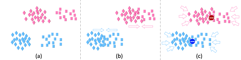
Figure 3: Comparison Between Average Domain Discrepancy and Multidomain Within-class Scatter. Colors denote classes and markers denote domains. (a) The distribution of data in the subspace $\mathbb{R}^{q}$ transformed from RKHS $\mathcal{H}$ using $\mathbf{W}^{0}$. (b) By minimizing average domain discrepancy, the resulting transformation $\mathbf{W}^{add}$ makes the means within each class closer. (c) By minimizing multidomain within-class scatter, the resulting transformation $\mathbf{W}^{mws}$ makes distribution of each class more compact towards the corresponding mean representation.

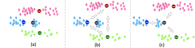
Figure 4: Comparison Between Average Class Discrepancy and Multidomain Between-class Scatter. Colors denote classes and markers denote domains. (a) The distribution of data in the subspace $\mathbb{R}^{q}$ transformed from RKHS $\mathcal{H}$ using $\mathbf{W}^{0}$. (b) By maximizing average class discrepancy, the resulting transformation $\mathbf{W}^{acd}$ treats the distances between each pair of mean representations equally and maximizes them; (c) By maximizing multidomain between-class scatter, the resulting transformation $\mathbf{W}^{mbs}$ maximizes the average distance between the overall mean and the mean representation of different classes. However, each distance is added a weight, which is proportional to the number of instances in the corresponding class. As a result, it is approximate equivalent to the scheme where one pools data of different domains of the same class together and trains classifier.

Appendix B Derivation of the Lagrangian

Since the objective

$$\operatorname*{arg\,max}_{\mathbf{B}}=\frac{\operatorname{tr}\left(\mathbf{B}^{T}\left(\beta\mathbf{F}+(1-\beta)\mathbf{P}\right)\mathbf{B}\right)}{\operatorname{tr}\left(\mathbf{B}^{T}(\gamma\mathbf{G}+\alpha\mathbf{Q}+\mathbf{K})\mathbf{B}\right)}$$ (20)

is invariant to re-scaling $\mathbf{B}\to\delta\mathbf{B}$, we rewrite (20) as a constrained optimization problem:

$$\operatorname*{arg\,max}_{\mathbf{B}} \;\operatorname{tr}\left(\mathbf{B}^{T}\left(\beta\mathbf{F}+(1-\beta)\mathbf{P}\right)\mathbf{B}\right)$$ (21)

$$s.t. \;\operatorname{tr}\left(\mathbf{B}^{T}(\gamma\mathbf{G}+\alpha\mathbf{Q}+\mathbf{K})\mathbf{B}\right)=1,$$ (22)

which yields the Lagrangian

$$\mathcal{L}= \operatorname{tr}\left(\mathbf{B}^{T}\left(\beta\mathbf{F}+(1-\beta)\mathbf{P}\right)\mathbf{B}\right)$$

$$-\operatorname{tr}\left(\left(\mathbf{B}^{T}(\gamma\mathbf{G}+\alpha\mathbf{Q}+\mathbf{K})\mathbf{B}-\mathbf{I}_{q}\right)\bm{\Gamma}\right),$$ (23)

where $\bm{\Gamma}$ is a diagonal matrix containing the Lagrange multipliers and $\mathbf{I}_{q}$ denotes the identity matrix of dimension $q$. Setting the derivative with respect to $\mathbf{B}$ in the Lagrangian (23) to zero yields the following generalized eigenvalue problem:

$$\left(\beta\mathbf{F}+(1-\beta)\mathbf{P}\right)\mathbf{B}=\left(\gamma\mathbf{G}+\alpha\mathbf{Q}+\mathbf{K}\right)\mathbf{B}\bm{\Gamma}.$$ (24)

Appendix C Proof of Theorem 2

Theorem 4.

Under assumptions 2 – 4, and further assuming that $\|\hat{f}\|_{\mathcal{H}_{\bar{k}}}\leq 1$ and $\|f^{*}\|_{\mathcal{H}_{\bar{k}}}\leq 1$, where $\hat{f}$ denotes the empirical risk minimizer, $f^{*}$ denotes the expected risk minimizer, then with probability at least $1-\delta$ there is

$$\mathbb{E}[\ell(\hat{f}(\tilde{X^{t}}\mathbf{W}),Y^{t})]-\mathbb{E}[\ell(f^{*}(\tilde{X^{t}}\mathbf{W}),Y^{t})]$$

$$\leq \ 4L_{\ell}L_{k_{\gamma}}U_{k^{\prime}_{x}}U_{k_{x}}\sqrt{\frac{\operatorname{tr}(\mathbf{B}^{T}\mathbf{KB})}{n}}+\sqrt{\frac{2\log 2\delta^{-1}}{n}},$$ (25)

where the expectations are taken over the joint distribution of the test domain $\mathbb{P}^{t}(X^{t},Y^{t})$, $n$ is the number of training samples, and $\mathbf{K}=\bm{\Phi}\bm{\Phi}^{T}$.

Proof.

First, we use the following result.

Theorem 5 (Generalization bound based on Rademacher complexity).

Define $\mathcal{A}=\{x\mapsto\ell(f(x),y):f\in\mathcal{H}\}$ to be the loss class, the composition of the loss function with each of the hypotheses. With probability at least $1-\delta$:

$$L(\hat{f})-L(f^{*})\leq 4\mathcal{R}_{n}(\mathcal{A})+\sqrt{\frac{2\log\frac{2}{\delta}}{n}},$$ (26)

where $L(\hat{f})$ denotes the expected test risk of the empirical risk minimizer, $L(\hat{f})$ denotes the expected test risk of the expected risk minimizer, $\mathcal{R}_{n}(\mathcal{A})$ denotes the Rademacher complexity of loss class $\mathcal{A}$, and $n$ denotes the number of training points.

By applying theorem 5, with probability at least $1-\delta$ there is

$$\mathbb{E}_{\mathbb{P}^{t}_{X}}[\ell(\hat{f}(\tilde{X^{t}}\mathbf{W}),Y^{t})]-\mathbb{E}_{\mathbb{P}^{t}_{X}}[\ell(f^{*}(\tilde{X^{t}}\mathbf{W}),Y^{t})]\leq 4\mathcal{R}_{n}(\mathcal{A})+\sqrt{\frac{2\log 2\delta^{-1}}{n}},$$ (27)

where $\mathcal{A}$ denotes the loss class $\{x\mapsto\ell(f(\mathbb{P},x),y):\|f\|_{\mathcal{H}_{\bar{k}}}\leq 1\}$, $\mathcal{R}_{n}(\cdot)$ denotes the Rademacher complexity and $n$ is the number of training points.

Since the loss function $\ell$ is $L_{\ell}$-Lipschitz in its first variable, there is

$$\mathcal{R}_{n}(\mathcal{A})=\mathcal{R}_{n}(\ell\circ f)\leq L_{\ell}\mathcal{R}_{n}(\mathcal{H}_{\bar{k}}).$$ (28)

To obtain the Rademacher complexity of $\mathcal{H}_{\bar{k}}$, i.e. $\mathcal{R}_{n}(\mathcal{H}_{\bar{k}})$, we adopt the following theorem.

Theorem 6 (Rademacher complexity of $L_{2}$ ball).

Let $\mathcal{F}=\{z\mapsto\langle w,z\rangle:\|w\|_{2}\leq B_{2}\}$ (bound on weight vectors). Assume $\mathbb{E}_{Z\sim p^{*}}\left[\|Z\|^{2}_{2}\right]\leq C^{2}_{2}$ (bound on spread of data points). Then

$$\mathcal{R}_{n}(\mathcal{F})\leq\frac{B_{2}C_{2}}{\sqrt{n}},$$ (29)

where $n$ denotes the number of training points.

According to the function class we restricted, $B_{2}$ in theorem 6 in our case is 1. For the bound of feature maps of data in $\mathcal{H}_{\bar{k}}$ (corresponds to $C_{2}$), there is

$$\ \left\|\bar{k}\left(\tilde{X^{t}}\mathbf{W},\cdot\right)\right\|$$ (30)

$$= \ \|\gamma_{k_{\gamma}}\left(\gamma(\mathbb{P}^{t})\right)\otimes k_{X}(X^{t},\cdot)\mathbf{W}\|$$ (31)

$$\leq \ L_{k_{\gamma}}\|\gamma(\mathbb{P}^{t})\|\|k_{X}(X^{t},\cdot)\mathbf{W}\|$$ (32)

$$\leq \ L_{k_{\gamma}}U_{k^{\prime}}U_{k}\|\mathbf{W}\|_{HS}.$$ (33)

Note that $\mathbf{W}=\bm{\Phi}^{T}\mathbf{B}$ and $\mathbf{K}=\bm{\Phi}\bm{\Phi}^{T}$ is invertible. It follows that $\operatorname{tr}(\mathbf{B}^{T}\mathbf{KB})$ defines a norm consistent with the Hilbert-Schmidt norm $\|\mathbf{W}\|_{HS}$. Therefore, by applying theorem 6, there is

$$\mathcal{R}_{n}(\mathcal{A})\leq L_{\ell}L_{k_{\gamma}}U_{k^{\prime}}U_{k}\sqrt{\frac{\operatorname{tr}(\mathbf{B}^{T}\mathbf{KB})}{n}}.$$ (34)

Combining it with (27) gives the results. ∎

Appendix D Proof of Theorem 3

Theorem 7.

Under assumptions 2 – 4, and assuming that all source sample sets are of the same size, i.e. $n^{s}=\bar{n}$ for $s=1,\dots,m$, then with probability at least $1-\delta$ there is

$$\sup_{\|f\|_{\mathcal{H}_{\bar{k}}}\leq 1}\left|\frac{1}{m}\sum^{m}_{s=1}\frac{1}{n^{s}}\sum^{n^{s}}_{i=1}\ell\left(f(\hat{\tilde{X}}^{s}_{i}\mathbf{W}),y^{s}_{i}\right)-\mathcal{E}(f,\infty)\right|$$

$$\leq U_{\ell}\left(\left(\frac{\log 2\delta^{-1}}{2m\bar{n}}\right)^{\frac{1}{2}}+\left(\frac{\log\delta^{-1}}{2m}\right)^{\frac{1}{2}}\right)+\sqrt{\operatorname{tr}(\mathbf{B}^{T}\mathbf{KB})}\left(c_{1}\left(\frac{\log 2\delta^{-1}m}{\bar{n}}\right)^{\frac{1}{2}}+c_{2}\left(\left(\frac{1}{m\bar{n}}\right)^{\frac{1}{2}}+\left(\frac{1}{m}\right)^{\frac{1}{2}}\right)\right)$$ (35)

where $c_{1}=2\sqrt{2}L_{\ell}U_{k_{x}}L_{k_{\gamma}}U_{k^{\prime}_{x}}$, $c_{2}=2L_{\ell}U_{k_{x}}U_{k_{\gamma}}$.

Proof.

Follow the idea in Blanchard et al. [2011], the supremum of the generalization error bound can be decomposed as

$$\ \sup_{\|f\|_{\mathcal{H}_{\bar{k}}}\leq 1}\left|\frac{1}{m}\sum^{m}_{s=1}\frac{1}{n^{s}}\sum^{n^{s}}_{i=1}\ell\left(f(\hat{\tilde{X}}^{s}_{i}\mathbf{W}),y^{s}_{i}\right)-\mathcal{E}(f,\infty)\right|$$

$$\leq \ \sup_{\|f\|_{\mathcal{H}_{\bar{k}}}\leq 1}\left|\frac{1}{m}\sum^{m}_{s=1}\frac{1}{n^{s}}\sum^{n^{s}}_{i=1}\left(\ell\left(f(\hat{\tilde{X}}^{s}_{i}\mathbf{W}),y^{s}_{i}\right)-\ell\left(f(\tilde{X}^{s}_{i}\mathbf{W}),y^{s}_{i}\right)\right)\right|$$ (36)

$$\ +\sup_{\|f\|_{\mathcal{H}_{\bar{k}}}\leq 1}\left|\frac{1}{m}\sum^{m}_{s=1}\frac{1}{n^{s}}\sum^{n^{s}}_{i=1}\ell\left(f(\tilde{X}^{s}_{i}\mathbf{W}),y^{s}_{i}\right)-\mathcal{E}(f,\infty)\right|$$ (37)

$$:= \ (I)+(II),$$ (38)

where $\hat{\tilde{X}}^{s}_{i}=(\hat{\mathbb{P}}^{s},x^{s}_{i})$, $\tilde{X}^{s}_{i}=(\mathbb{P}^{s},x^{s}_{i})$.

Bound of term (I)

According to the assumption that the loss $\ell$ is $L_{\ell}$ -Lipschitz in its first variable, we have

$$(I)\leq L_{\ell}\sup_{\|f\|_{\mathcal{H}_{\bar{k}}}\leq 1}\frac{1}{m}\sum^{m}_{s=1}\frac{1}{n^{s}}\sum^{n^{s}}_{i=1}\left|f(\hat{\tilde{X}}^{s}_{i}\mathbf{W})-f(\tilde{X}^{s}_{i}\mathbf{W})\right|$$ (39)

$$\leq L_{\ell}\sup_{\|f\|_{\mathcal{H}_{\bar{k}}}\leq 1}\frac{1}{m}\sum^{m}_{s=1}\left\|f\left((\hat{\mathbb{P}}^{s},\cdot)\mathbf{W}\right)-f\left((\mathbb{P}^{s},\cdot)\mathbf{W}\right)\right\|_{\infty}$$ (40)

For any $x\in\mathcal{X}$ and $\|f\|_{\mathcal{H}_{\bar{k}}}\leq 1$, using the reproducing property of the kernel $\bar{k}$ and Cauchy-Schwarz inequality, we have

$$\left|f\left((\hat{\mathbb{P}}^{s},x)\mathbf{W}\right)-f\left((\mathbb{P}^{s},x)\mathbf{W}\right)\right| =\left|\left\langle\bar{k}\left((\hat{\mathbb{P}}^{s},x)\mathbf{W},\cdot\right)-\bar{k}\left((\mathbb{P}^{s},x)\mathbf{W},\cdot\right),f\right\rangle\right|$$ (41)

$$\leq\left\|f\right\|\left\|\bar{k}\left((\hat{\mathbb{P}}^{s},x)\mathbf{W},\cdot\right)-\bar{k}\left((\mathbb{P}^{s},x)\mathbf{W},\cdot\right)\right\|$$ (42)

According to the assumption, there is $\|f\|\leq 1$. For the second term in (42) we have

$$\left\|\bar{k}\left((\hat{\mathbb{P}}^{s},x)\mathbf{W},\cdot\right)-\bar{k}\left((\mathbb{P}^{s},x)\mathbf{W},\cdot\right)\right\|$$ (43)

$$= \left\|\gamma_{k_{\gamma}}\left(\gamma(\hat{\mathbb{P}}^{s})\right)\otimes k_{X}(x,\cdot)\mathbf{W}-\gamma_{k_{\gamma}}\left(\gamma(\mathbb{P}^{s})\right)\otimes k_{X}(x,\cdot)\mathbf{W}\right\|$$ (44)

$$\leq \left\|\gamma_{k_{\gamma}}\left(\gamma(\hat{\mathbb{P}}^{s})\right)\otimes k_{X}(x,\cdot)-\gamma_{k_{\gamma}}\left(\gamma(\mathbb{P}^{s})\right)\otimes k_{X}(x,\cdot)\right\|\left\|\mathbf{W}\right\|_{HS}$$ (45)

$$= \left\|\mathbf{W}\right\|_{HS}\left(\left\langle\bar{k}((\hat{\mathbb{P}}^{s},x),\cdot)-\bar{k}((\mathbb{P}^{s},x),\cdot),\bar{k}((\hat{\mathbb{P}}^{s},x),\cdot)-\bar{k}((\mathbb{P}^{s},x),\cdot)\right\rangle\right)^{\frac{1}{2}}$$ (46)

$$\leq \left\|\mathbf{W}\right\|_{HS}k(x,x)^{\frac{1}{2}}\left(k_{\gamma}(\gamma(\mathbb{P}^{s}),\gamma(\mathbb{P}^{s}))+k_{\gamma}(\gamma(\hat{\mathbb{P}}^{s}),\gamma(\hat{\mathbb{P}}^{s}))-2k_{\gamma}(\gamma(\mathbb{P}^{s}),\gamma(\hat{\mathbb{P}}^{s}))\right)^{\frac{1}{2}}$$ (47)

$$\leq U_{k}\left\|\mathbf{W}\right\|_{HS}\left\|\gamma_{k_{\gamma}}\left(\gamma(\mathbb{P}^{s})\right)-\gamma_{k_{\gamma}}\left(\gamma(\hat{\mathbb{P}}^{s})\right)\right\|$$ (48)

$$\leq U_{k}L_{k_{\gamma}}\left\|\mathbf{W}\right\|_{HS}\left\|\gamma(\hat{\mathbb{P}}^{s})-\gamma(\mathbb{P}^{s})\right\|.$$ (49)

Combining (42), (49) and $\left\|f\right\|\leq 1$, there is

$$\left|f\left((\hat{\mathbb{P}}^{s},x)\mathbf{W}\right)-f\left((\mathbb{P}^{s},x)\mathbf{W}\right)\right|\leq U_{k}L_{k_{\gamma}}\left\|\mathbf{W}\right\|_{HS}\left\|\gamma(\hat{\mathbb{P}}^{s})-\gamma(\mathbb{P}^{s})\right\|.$$ (50)

Now we derive the bound on $\left\|\gamma(\hat{\mathbb{P}}^{s})-\gamma(\mathbb{P}^{s})\right\|$. For independent real zero-mean random variables $x_{1},\dots,x_{n}$ such that $|x_{i}|\leq C$ for $i=1,\dots,n$, Hoeffding’s inequality states that $\forall\epsilon>0$:

$$\text{P}\left[\left|\frac{1}{n}\sum^{n}_{i=1}x_{i}\right|>\epsilon\right]\leq 2\exp\left(-\frac{n\epsilon^{2}}{2C^{2}}\right).$$ (51)

Set the $\delta=2\exp\left(-\frac{n\epsilon^{2}}{2C^{2}}\right)$, then with probability at least $1-\delta$:

$$\left|\frac{1}{n}\sum^{n}_{i=1}x_{i}\right|<\sqrt{2}C\sqrt{\frac{\log 2\delta^{-1}}{n}}.$$ (52)

Similar result holds for zero-mean independent random variables $\phi(x_{1}),\dots,\phi(x_{n})$ with values in a separable complex Hilbert space and such that $\|\phi(x_{i})\|\leq C$, for $i=1,\dots,n$:

$$\left\|\frac{1}{n}\sum^{n}_{i=1}\phi(x_{i})\right\|<\sqrt{2}C\sqrt{\frac{\log 2\delta^{-1}}{n}}.$$ (53)

For independent uncentered variables $\phi^{\prime}(x_{i})$ with mean $M$, bounded by $C$. Let $\phi(x_{i})=\phi^{\prime}(x_{i})-M$ denote the re-centered variables, now bounded at worst by $2C$ by the triangle inequality. Set $\delta=2\exp\left(-\frac{n\epsilon^{2}}{8C^{2}}\right)$, we obtain with probability at least $1-\delta$ that:

$$\left\|\frac{1}{n}\sum^{n}_{i=1}\phi^{\prime}(x_{i})-M\right\|<2\sqrt{2}C\sqrt{\frac{\log 2\delta^{-1}}{n}}$$ (54)

Based on the result of (54), we have

$$\left\|\gamma(\hat{\mathbb{P}}^{s})-\gamma(\mathbb{P}^{s})\right\|=\left\|\frac{1}{n^{s}}\sum^{n}_{i=1}\phi^{\prime}(x^{s}_{i})-\mathbb{E}_{X\sim\mathbb{P}^{s}}[\phi^{\prime}(X)]\right\|\leq 3U_{k^{\prime}}\sqrt{\frac{\log 2\delta^{-1}}{\bar{n}}}$$ (55)

Combining (50) and (55) we have

$$\sup_{\|f\|_{\mathcal{H}_{\bar{k}}}\leq 1}\left\|f\left((\hat{\mathbb{P}}^{s},\cdot)\mathbf{W}\right)-f\left((\mathbb{P}^{s},\cdot)\mathbf{W}\right)\right\|_{\infty}\leq 2\sqrt{2}U_{k}L_{k_{\gamma}}U_{k^{\prime}}\left\|\mathbf{W}\right\|_{HS}\sqrt{\frac{\log 2\delta^{-1}}{\bar{n}}}$$ (56)

Conditionally to the draw of $\{\mathbb{P}^{s}\}_{1\leq s\leq m}$, we can apply (56) to each $(\mathbb{P}^{s},\hat{\mathbb{P}}^{s})$ the the union bound over $s=1,\dots,m$ to get that with probability at least $1-\delta$:

$$(I)\leq 2\sqrt{2}L_{\ell}U_{k}L_{k_{\gamma}}U_{k^{\prime}}\left\|\mathbf{W}\right\|_{HS}\sqrt{\frac{\log 2\delta^{-1}+\log m}{\bar{n}}}$$ (57)

Bound of term (II)

This section follows the idea of Blanchard et al. [2011] so steps of proof that are largely unchanged are omitted. First, we define the conditional (idealized) test error for a given test distribution $\mathbb{P}^{t}_{XY}$ as

$$\mathcal{E}(f,\infty|\mathbb{P}^{t}_{XY}):=\mathbb{E}_{(X^{t},Y^{t})\sim\mathbb{P}^{t}_{XY}}\left[\ell\left(f(\tilde{X}^{t}\mathbf{W}),Y^{t}\right)\right],$$ (58)

where $\tilde{X}^{t}=(P^{t}_{X},X^{t})$.

Then (II) is further decomposed as

$$(II)\leq \frac{1}{m}\sum^{m}_{s=1}\frac{1}{n^{s}}\sum^{n^{s}}_{i=1}\left(\ell\left(f(\tilde{X}^{s}_{i}\mathbf{W}),y^{s}_{i}\right)-\mathcal{E}(f,\infty|\mathbb{P}^{s}_{XY})\right)+\frac{1}{m}\sum^{m}_{s=1}\left(\mathcal{E}(f,\infty|\mathbb{P}^{s}_{XY})-\mathcal{E}(f,\infty)\right)$$ (59)

$$:= (IIa)+(IIb)$$ (60)

Bound of term (IIa)

In the case where conditioning on $\{\mathbb{P}^{s}_{XY}\}_{1\leq s\leq m}$, the observations in $\mathcal{D}=\{(x^{s}_{i},y^{s}_{i})\}^{m,n^{s}}_{s=1,i=1}$ are now independent (but not identically distributed) for this conditional distribution. We can thus apply the McDiarmid inequality to the function

$$\zeta\left(\mathcal{D}\right):=\sup_{\|f\|_{\mathcal{H}_{\bar{k}}}\leq 1}\frac{1}{m}\sum^{m}_{s=1}\frac{1}{n^{s}}\sum^{n^{s}}_{i=1}\left(\ell\left(f(\tilde{X}^{s}_{i}\mathbf{W}),y^{s}_{i}\right)-\mathcal{E}(f,\infty|\mathbb{P}^{s}_{XY})\right).$$ (61)

When $n^{s}=n^{s^{\prime}}=\bar{n}$ for all $s,s^{\prime}$, that with probability $1-\delta$ over the draw of $\mathcal{D}$, it holds

$$\left|\zeta-\mathbb{E}\left[\zeta|\{\mathbb{P}^{s}_{XY}\}_{1\leq s\leq m}\right]\right|\leq U_{l}\sqrt{\frac{\log{2\delta^{-1}}}{2m\bar{n}}}.$$ (62)

Then by the standard symmetrization technique, $\mathbb{E}\left[\zeta|\{\mathbb{P}^{s}_{XY}\}_{1\leq s\leq m}\right]$ can be bounded via Rademacher complexity as:

$$\mathbb{E}\left[\zeta|\{\mathbb{P}^{s}_{XY}\}_{1\leq s\leq m}\right]\leq \frac{2}{m}\mathbb{E}_{(x^{s}_{i},y^{s}_{i})}\mathbb{E}_{(\epsilon^{s}_{i})}\left[\sup_{\|f\|_{\mathcal{H}_{\bar{k}}}\leq 1}\sum^{m}_{s=1}\frac{1}{n^{s}}\sum^{n^{s}}_{i=1}\epsilon^{s}_{i}\left(\ell\left(f(\tilde{X}^{s}_{i}\mathbf{W}),y^{s}_{i}\right)\right)|\{\mathbb{P}^{s}_{XY}\}_{1\leq s\leq m}\right]$$ (63)

$$\leq 2L_{\ell}U_{k}U_{k_{\gamma}}\left\|\mathbf{W}\right\|_{HS}\sqrt{\frac{1}{m\bar{n}}},$$ (64)

where the last inequality is from the bound of the Rademacher complexity of the loss class $\ell\circ f$.

Bound of term (IIb)

Since the $\{\mathbb{P}^{s}_{XY}\}_{1\leq s\leq m}$ are i.i.d., the McDiarmid inequality can be applied to the function

$$\xi\left(\{\mathbb{P}^{s}_{XY}\}_{1\leq s\leq m}\right):=\sup_{\|f\|_{\mathcal{H}_{\bar{k}}}\leq 1}\frac{1}{m}\sum^{m}_{s=1}\left(\mathcal{E}(f,\infty|\mathbb{P}^{s}_{XY})-\mathcal{E}(f,\infty)\right),$$ (65)

then one obtains that with probability $1-\delta$ over the draw of $\{\mathbb{P}^{s}_{XY}\}_{1\leq s\leq m}$, it holds

$$\left|\xi-\mathbb{E}[\xi]\right|\leq U_{\ell}\sqrt{\frac{\log\delta^{-1}}{2m}}.$$ (66)

Similarly, by the standard symmetrization technique, $\mathbb{E}[\xi]$ is bounded as

$$\mathbb{E}[\xi]\leq \frac{2}{m}\mathbb{E}_{\{\mathbb{P}^{s}_{XY}\}_{1\leq s\leq m}}\mathbb{E}_{(X^{s},Y^{s})_{1\leq s\leq m}}\mathbb{E}_{(\epsilon^{s})_{1\leq s\leq m}}\left[\sup_{\|f\|_{\mathcal{H}_{\bar{k}}}\leq 1}\sum^{m}_{s=1}\epsilon^{s}\ell\left(f(\tilde{X}^{s}\mathbf{W}),Y^{s}\right)\right]$$ (67)

$$\leq 2L_{\ell}U_{k}U_{k_{\gamma}}\left\|\mathbf{W}\right\|_{HS}\sqrt{\frac{1}{m}},$$ (68)

where the last inequality is again from the bound of the Rademacher complexity of the loss class $\ell\circ f$.

Finally, $\mathbf{W}=\bm{\Phi}^{T}\mathbf{B}$ and $\mathbf{K}=\bm{\Phi}\bm{\Phi}^{T}$ is invertible. It follows that $\operatorname{tr}(\mathbf{B}^{T}\mathbf{KB})$ defines a norm consistent with the Hilbert-Schmidt norm $\|\mathbf{W}\|_{HS}$. By combining the above results we obtain the announced result. ∎

Appendix E Experimental Configurations

Due to the difference in techniques adopted in different methods, there is/are different hyper-parameter(s) in each method require tuning in the experiments.

• 1NN: since there is no hyper-parameter to be determined in 1NN, instances in source domains are directly combined for training. Then we apply the trained model on target domains and report the test accuracy.

• SVM: the regularization coefficient $C$ requires tuning in SVM. $C\in\{0.1,0.5,1.0,2.0,5.0,10.0\}$ are validated in the experiments.

• KPCA and KFD: the kernel width $\sigma_{k}$ requires tuning. $\sigma_{k}\in\{0.1d_{M},0.2d_{M},0.5d_{M},d_{M},2d_{M},5d_{M}\}$, where $d_{M}=\text{median}\left(\|\bm{x}_{i}-\bm{x}_{j}\|^{2}_{2}\right),\forall\bm{x}_{i},\bm{x}_{j}\in\mathcal{D}$, are validated.

• E-SVM: four hyper-parameters ($\lambda_{1},\lambda_{2},C_{1},C_{2}$) require tuning. $\lambda_{1}\in\{0.1,1,10\}$, $\lambda_{2}\in\{0.5\lambda_{1},1\lambda_{1},2\lambda_{1}\}$, and $C_{1},C_{2}\in\{0.1,1,10\}$ are validated.

• CCSA: two hyper-parameters ($lr,\alpha$) require tuning. learning rate $lr\in\{0.5,1.0,1.5\}$ and $\alpha\in\{0.1,0.25,0.4\}$ are validated.

• DICA: Two parameters ($\lambda$, $\epsilon$) require tuning. $\lambda\in\{1\mathrm{e}{-3},1\mathrm{e}{-2},1\mathrm{e}{-1},1.0,1\mathrm{e}{1},1\mathrm{e}{2},1\mathrm{e}{3}\}$
  and $\epsilon\in\{1\mathrm{e}{-3},1\mathrm{e}{-2},1\mathrm{e}{-1},1.0,1\mathrm{e}{1},1\mathrm{e}{2},1\mathrm{e}{3}\}$ were validated.

• SCA: Two parameters ($\beta,\delta$) require tuning. $\beta\in\{0.1,0.3,0.5,0.7,0.9\}$,
  $\delta\in\{1\mathrm{e}{-3},1\mathrm{e}{-2},1\mathrm{e}{-1},1.0,1\mathrm{e}{1},1\mathrm{e}{2},1\mathrm{e}{3},1\mathrm{e}{4},1\mathrm{e}{5},1\mathrm{e}{6}\}$ were validated.

• CIDG: Three hyper-parameters ($\beta,\alpha,\gamma$) require tuning. $\beta\in\{0.1,0.3,0.5,0.7,0.9\}$,
  $\gamma\in\{1\mathrm{e}{-3},1\mathrm{e}{-2},1\mathrm{e}{-1},1,1\mathrm{e}{1},1\mathrm{e}{2},1\mathrm{e}{3},1\mathrm{e}{4},1\mathrm{e}{5},1\mathrm{e}{6}\}$, and
  $\alpha\in\{1,1\mathrm{e}{1},1\mathrm{e}{2},1\mathrm{e}{3},1\mathrm{e}{4},1\mathrm{e}{5},1\mathrm{e}{6},1\mathrm{e}{7},1\mathrm{e}{8},1\mathrm{e}{9}\}$, were validated.

• MDA: Three hyper-parameters ($\beta,\alpha,\gamma$) require tuning. $\beta\in\{0.1,0.3,0.5,0.7,0.9\}$,
  $\gamma\in\{1\mathrm{e}{-3},1\mathrm{e}{-2},1\mathrm{e}{-1},1.0,1\mathrm{e}{1},1\mathrm{e}{2},1\mathrm{e}{3},1\mathrm{e}{4},1\mathrm{e}{5},1\mathrm{e}{6}\}$, and
  $\alpha\in\{1,1\mathrm{e}{1},1\mathrm{e}{2},1\mathrm{e}{3},1\mathrm{e}{4},1\mathrm{e}{5},1\mathrm{e}{6},1\mathrm{e}{7},1\mathrm{e}{8},1\mathrm{e}{9}\}$, were validated.

For feature extraction methods (i.e., KPCA and KFD) and kernel-based DG methods (i.e., DICA, SCA, CIDG, and MDA), in real data experiments, different number of leading eigenvectors (corresponds to the dimension of the transformed subspace) that contribute to certain proportions (i.e. $\{0.2,0.4,0.6,0.8,0.92,$ $0.94,0.96,0.98\}$) of the sum of all eigenvalues are tested and the highest accuracies are reported for each method.

Appendix F Synthetic Experimental Results Visualization

In this section, we show the data distribution of source domains in the transformed domain-invariant subspace $\mathbb{R}^{q}$ of the synthetic experiment for kernel-based DG methods: SCA, CIDG, MDA, which are proposed for classification problems. The results are given in Figure 5 and 6.

We observe from the results that: 1) the transformation learned from MDA performs the best in terms of the separation of different classes of target domains; 2) the overlapped region in source domains(green and red classes) is handled slightly better in MDA than in CIDG; 3) SCA has difficulty in separating instances of different classes in part of the cases.

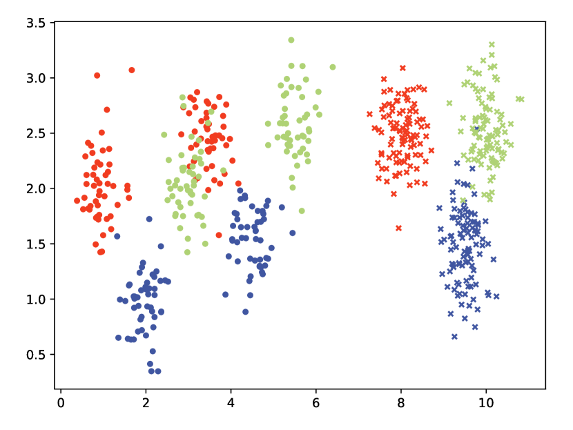
(a) (2a, 2a) Raw data

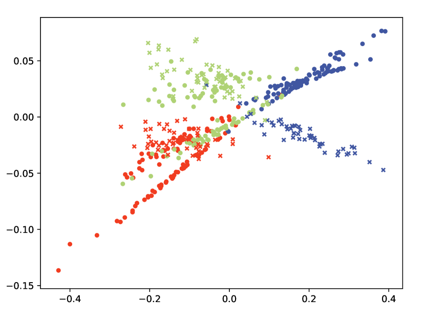
(b) SCA(79.33%)

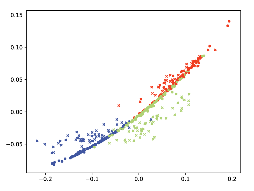
(c) CIDG(90.67%)

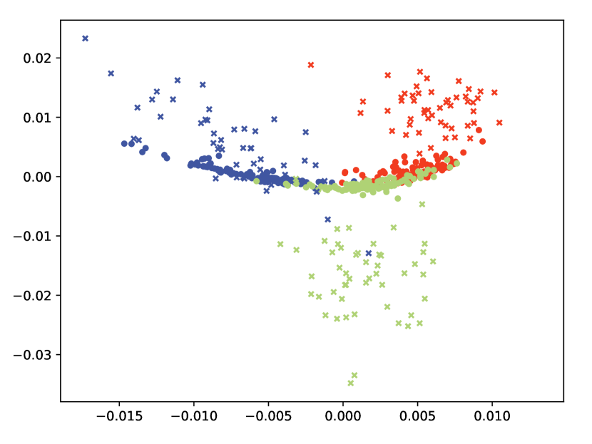
(d) MDA(96.67%)

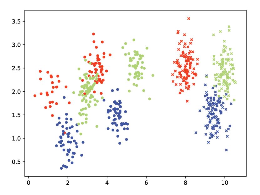
(e) (2b, 2a) Raw data

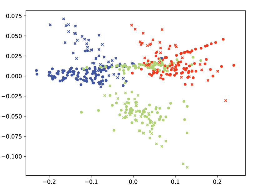
(f) SCA(72.00%)

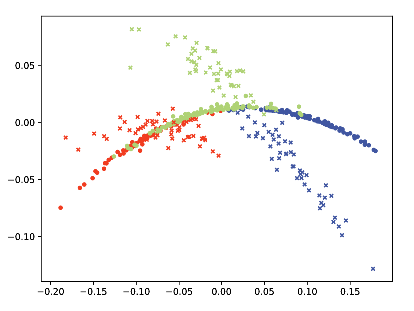
(g) CIDG(87.33%)

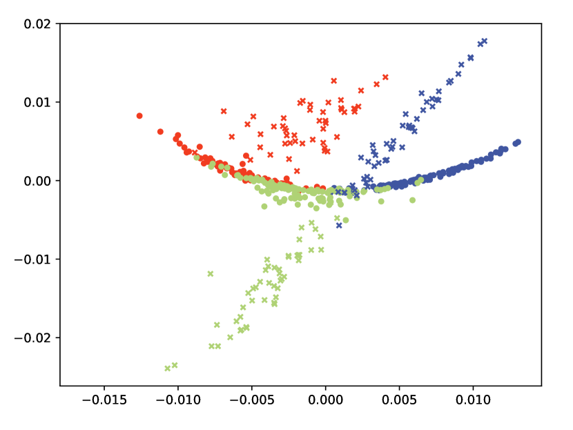
(h) MDA(96.00%)

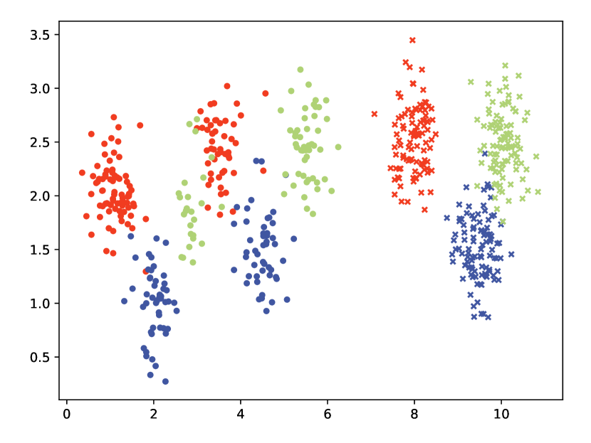
(i) (2c, 2a) Raw data

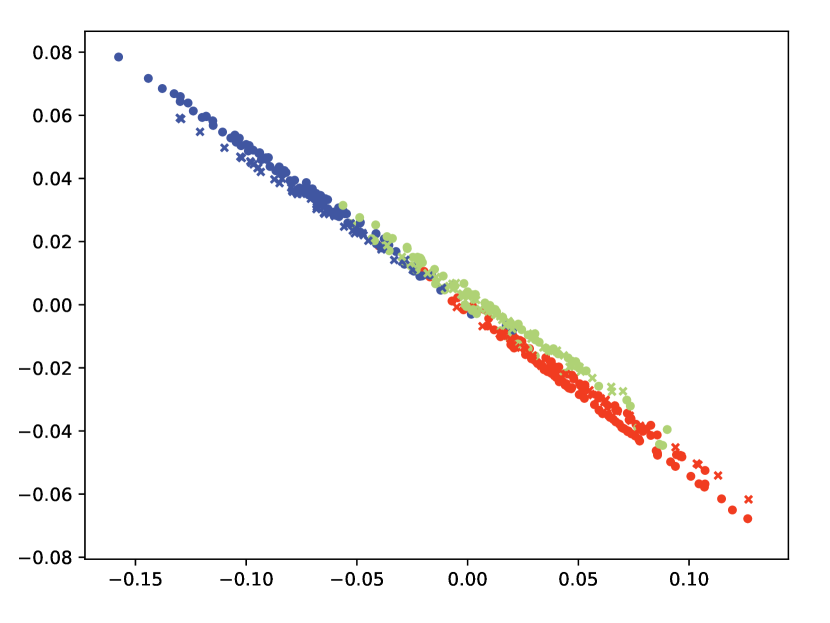
(j) SCA(84.67%)

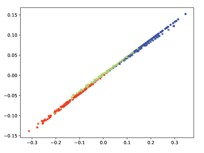
(k) CIDG(74.67%)

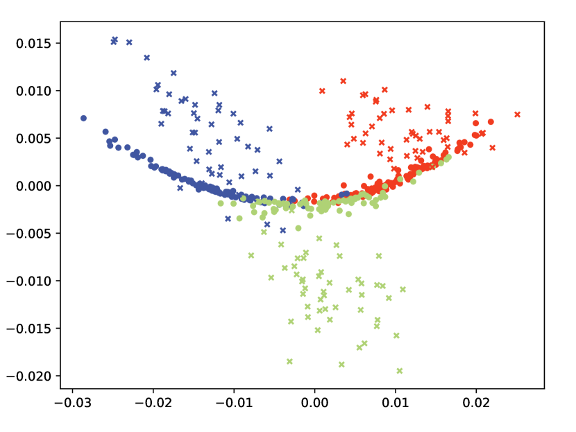
(l) MDA(97.33%)

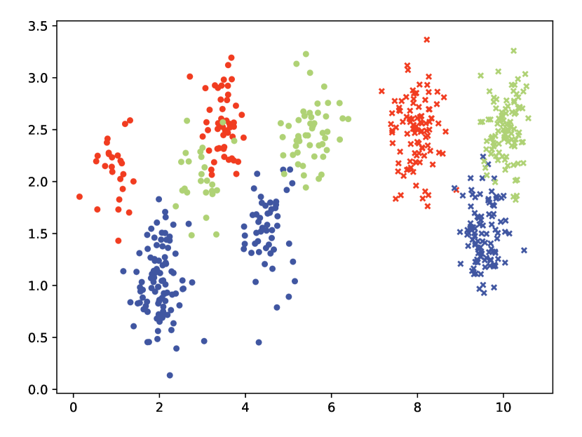
(m) (2d, 2a) Raw data

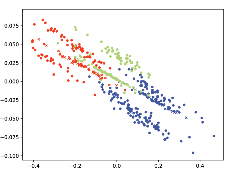
(n) SCA(57.33%)

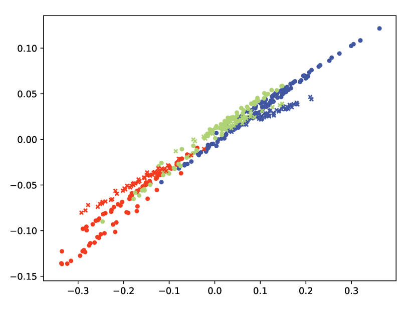
(o) CIDG(77.33%)

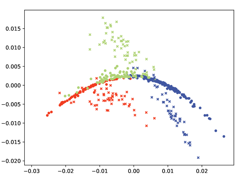
(p) MDA(94.00%)

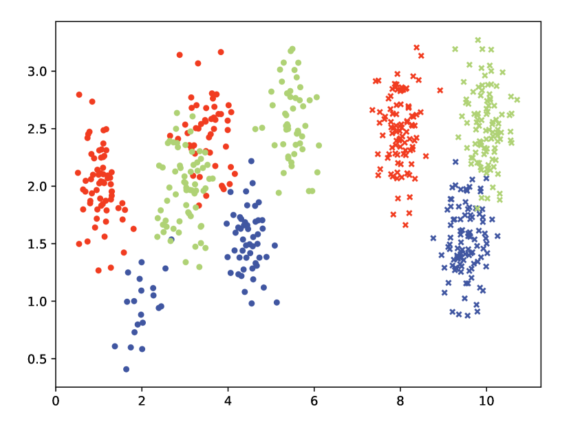
(q) (2e, 2a) Raw data

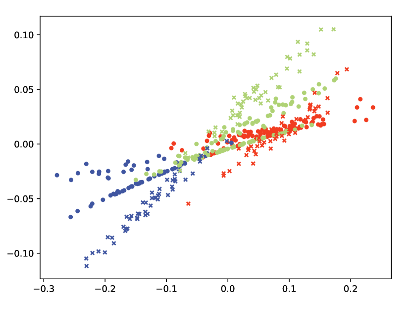
(r) SCA(76.00%)

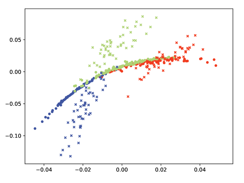
(s) CIDG(86.67%)

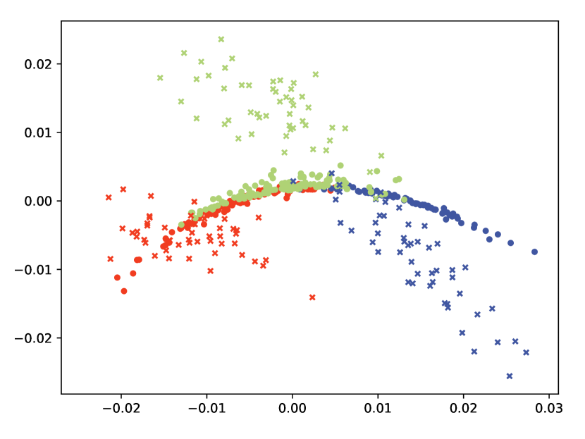
(t) MDA(94.00%)

Figure 5: Visualization of transformed data in $\mathbb{R}^{q}$ of cases (2a, 2a), (2b, 2a), (2c, 2a), (2d, 2a), (2e, 2a). Each row corresponds to a case of class-prior distributions. Each column corresponds to a DG methods. The first column shows the distribution of the raw data. Different colors denote different classes. Circle marker denotes the data of source domain and cross marker denotes the data of target domain.

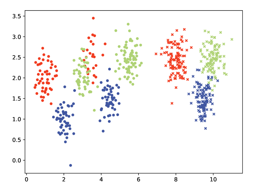
(a) (2a, 2b) Raw data

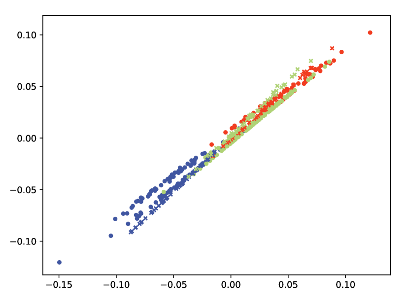
(b) SCA(59.33%)

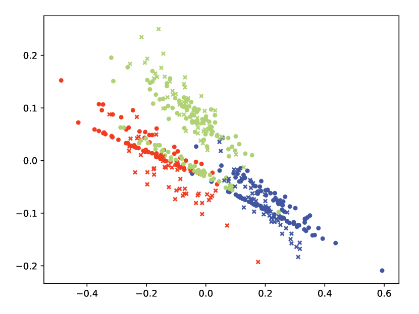
(c) CIDG(83.33%)

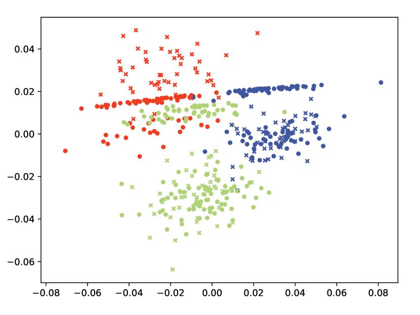
(d) MDA(91.33%)

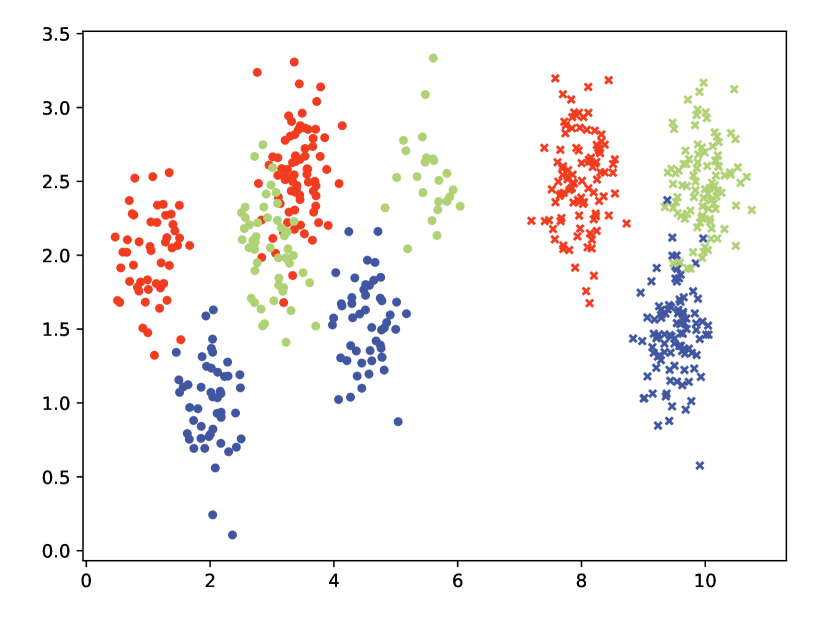
(e) (2a, 2c) Raw data

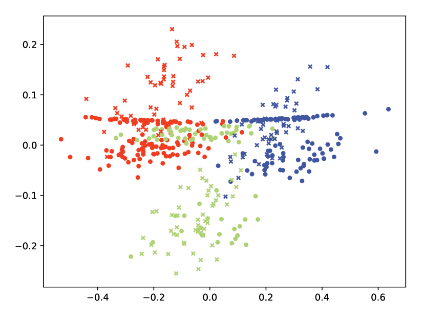
(f) SCA(84.67%)

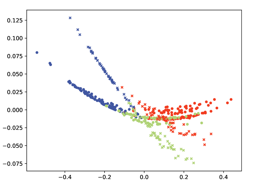
(g) CIDG(92.00%)

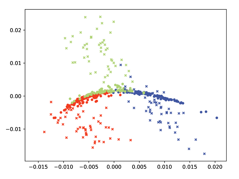
(h) MDA(95.33%)

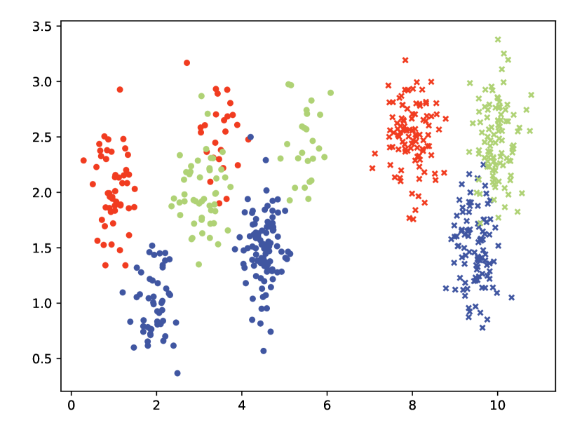
(i) (2a, 2d) Raw data

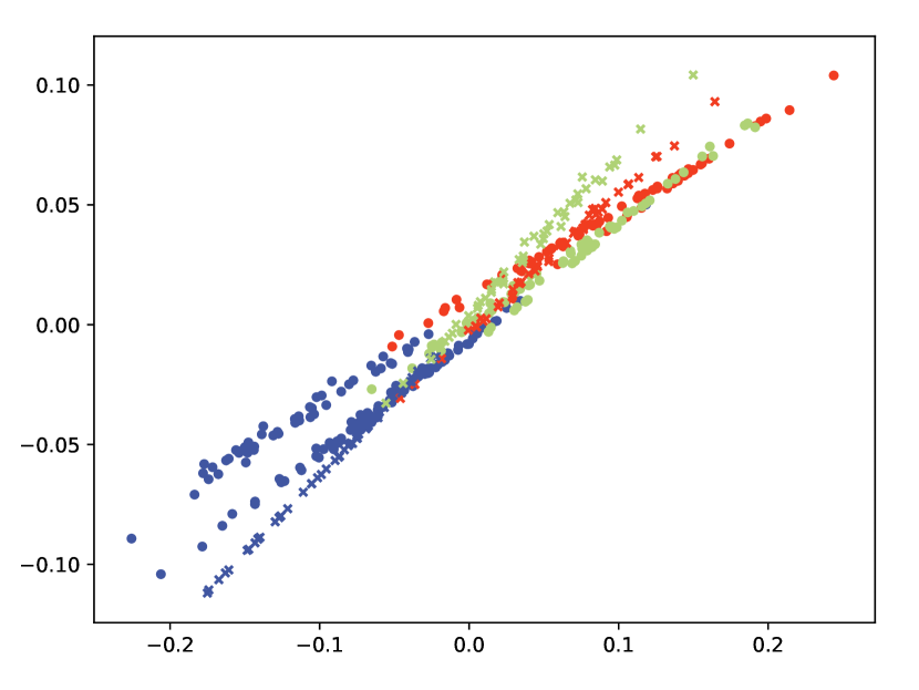
(j) SCA(61.33%)

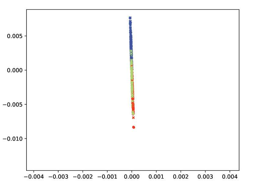
(k) CIDG(82.00%)

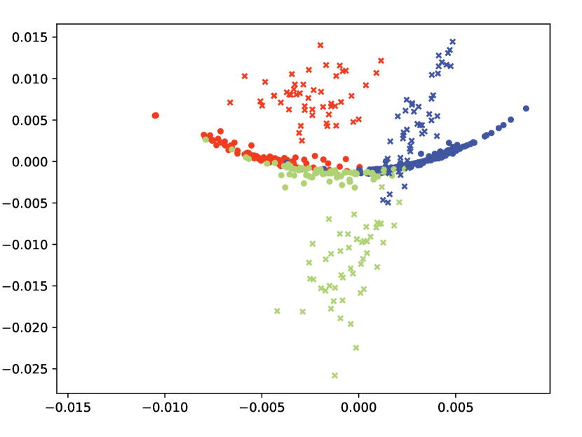
(l) MDA(94.00%)

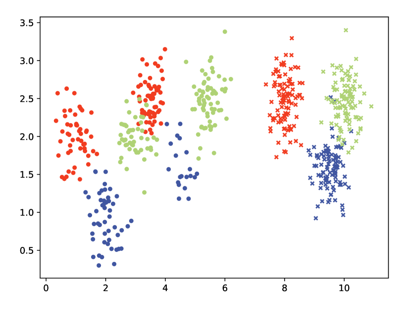
(m) (2a, 2e) Raw data

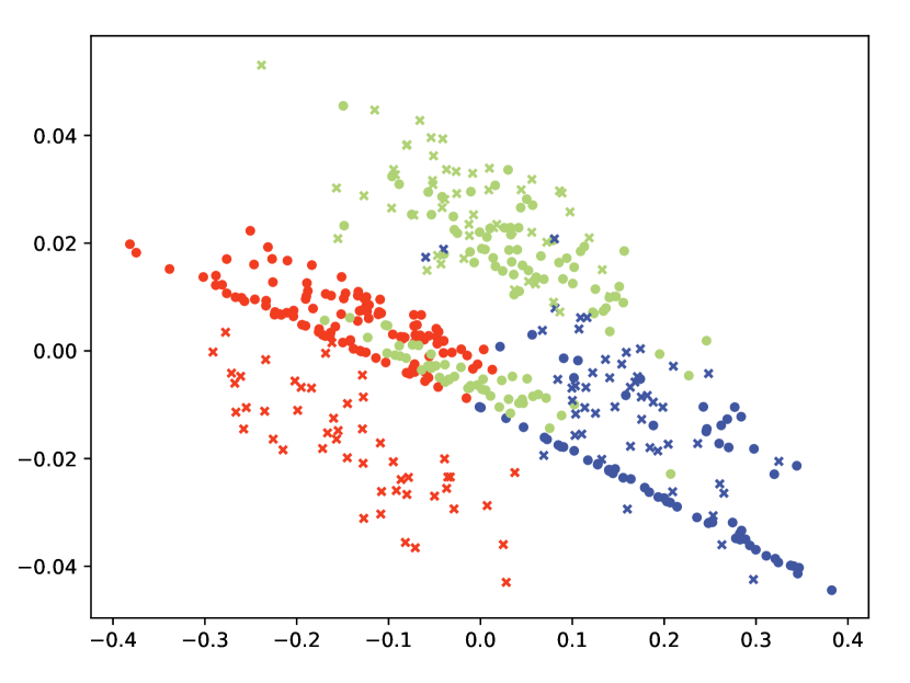
(n) SCA(81.33%)

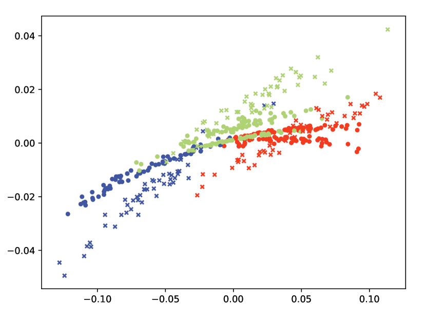
(o) CIDG(86.00%)

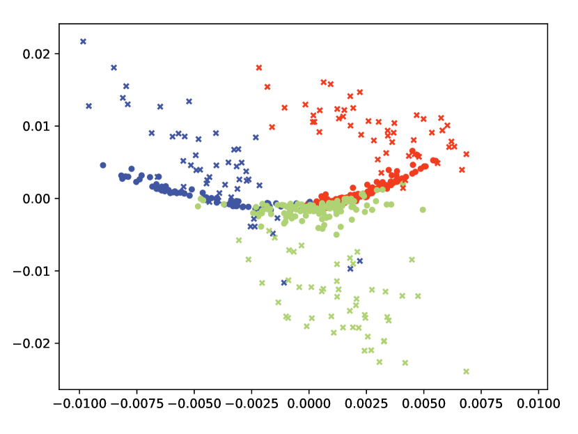
(p) MDA(94.00%)

Figure 6: Visualization of transformed data in $\mathbb{R}^{q}$ of cases (2a, 2b), (2a, 2c), (2a, 2d), (2a, 2e). Each row corresponds to a case of class-prior distributions. Each column corresponds to a DG methods. The first column shows the distribution of the raw data. Different colors denote different classes. Circle marker denotes the data of source domain and cross marker denotes the data of target domain.

Appendix G Related Work

Compared with domain adaptation, domain generalization is a younger line of research. Blanchard et al. [2011] are the first to formalize the domain generalization of classification tasks. Motivated by automatic gating of flow cytometry data, they adopted kernel-based methods and derived the dual of a kind of cost-sensitive SVM to solve for the optimal decision function. A feature projection-based method called Domain Invariant Component Analysis (DICA; [Muandet et al., 2013]) was then proposed in 2013. DICA was the first to bring the idea of learning a shared subspace into domain generalization. It finds a transformation to a subspace in which the differences between marginal distributions $\mathbb{P}(X)$ over domains are minimized while preserving the functional relationship between $Y$ and $X$.

Along this line, subsequent feature projection-based methods have been proposed. Scatter Component Analysis (SCA; [Ghifary et al., 2017]) is the first unified framework for both domain adaptation and domain generalization. It combines domain scatter, kernel principal component analysis and kernel Fisher discriminant analysis into an objective and trades between them to learn the transformation. Unlike previous works, the authors of Conditional Invariant Domain Generalization (CIDG; [Li et al., 2018b]) are the first to analyze domain generalization of classification tasks from causal perspective and thus consider more general cases where both $\mathbb{P}(Y|X)$ and $\mathbb{P}(X)$ vary across domains. They combine total scatter of class-conditional distributions, scatter of class prior-normalized marginal distributions, and kernel Fisher discriminant analysis to achieve the goal of domain generalization.

Besides the aforementioned methods in general, domain generalization problem also attracted extensive attention of computer vision community. Khosla et al. [2012] proposed a max-margin framework (Undo-Bias) in which each domain is assumed to be controlled by the sum of the visual world and a bias. A modified SVM-based method is adopted for solving the weights and biases in the model. Unbiased Metric Learning (UML; [Fang et al., 2013]), which is based on a learning-to-rank framework, first learns a set of distance metrics and then validate to select the one with best generalization ability. Xu et al. [2014] adopted exemplar-SVM and introduced a nuclear norm based regularizer into the objective to learn a set of more robust examplar-SVMs for domain generalization purpose. Ghifary et al. [2015] introduced Multi-task Autoencoder (MTAE), a feature learning algorithm that uses a multi-task strategy to learn unbiased object features, where the task is the data reconstruction. More recently, domain generalization methods based on deep neural networks [Motiian et al., 2017, Li et al., 2017, 2018a, 2018c] were proposed to cope with the problem induced by distribution shift.

References

• Barrio et al. [1999] Eustasio Del Barrio, J A Cuestaalbertos, Carlos Matran, and Jes U S M Rodriguezrodriguez. Tests of goodness of fit based on the $l_{2}$-wasserstein distance. Annals of Statistics, 27(4):1230–1239, 1999.
• Blanchard et al. [2011] Gilles Blanchard, Gyemin Lee, and Clayton Scott. Generalizing from several related classification tasks to a new unlabeled sample. In Advances in Neural Information Processing Systems (NIPS), pages 2178–2186, 2011.
• Choi et al. [2010] Myung Jin Choi, Joseph J Lim, Antonio Torralba, and Alan S Willsky. Exploiting hierarchical context on a large database of object categories. In Proceedings of IEEE Conference on Computer Vision and Pattern Recognition (CVPR), pages 129–136, 2010.
• Daniušis et al. [2010] Povilas Daniušis, Dominik Janzing, Joris Mooij, Jakob Zscheischler, Bastian Steudel, Kun Zhang, and Bernhard Schölkopf. Inferring deterministic causal relations. In Proceedings of the Twenty-Sixth Conference on Uncertainty in Artificial Intelligence (UAI 2010), pages 143–150, 2010.
• Donahue et al. [2014] Jeff Donahue, Yangqing Jia, Oriol Vinyals, Judy Hoffman, Ning Zhang, Eric Tzeng, and Trevor Darrell. Decaf: A deep convolutional activation feature for generic visual recognition. In Proceedings of the 31st International Conference on Machine Learning (ICML 2014), pages 647–655, 2014.
• Everingham et al. [2010] Mark Everingham, Luc Van Gool, Christopher KI Williams, John Winn, and Andrew Zisserman. The pascal visual object classes (voc) challenge. International Journal of Computer Vision, 88(2):303–338, 2010.
• Fang et al. [2013] Chen Fang, Ye Xu, and Daniel N Rockmore. Unbiased metric learning: On the utilization of multiple datasets and web images for softening bias. In Proceedings of the IEEE International Conference on Computer Vision (ICCV), pages 1657–1664, 2013.
• Ghifary et al. [2015] Muhammad Ghifary, W Bastiaan Kleijn, Mengjie Zhang, and David Balduzzi. Domain generalization for object recognition with multi-task autoencoders. In Proceedings of the IEEE International Conference on Computer Vision (ICCV), pages 2551–2559, 2015.
• Ghifary et al. [2017] Muhammad Ghifary, David Balduzzi, W Bastiaan Kleijn, and Mengjie Zhang. Scatter component analysis: A unified framework for domain adaptation and domain generalization. IEEE Transactions on Pattern Analysis and Machine Intelligence, 39(7):1414–1430, 2017.
• Girshick et al. [2014] Ross Girshick, Jeff Donahue, Trevor Darrell, and Jitendra Malik. Rich feature hierarchies for accurate object detection and semantic segmentation. In Proceedings of IEEE Conference on Computer Vision and Pattern Recognition (CVPR), pages 580–587, 2014.
• Gong et al. [2012] Boqing Gong, Yuan Shi, Fei Sha, and Kristen Grauman. Geodesic flow kernel for unsupervised domain adaptation. In Proceedings of IEEE Conference on Computer Vision and Pattern Recognition (CVPR), pages 2066–2073, 2012.
• Gong et al. [2016] Mingming Gong, Kun Zhang, Tongliang Liu, Dacheng Tao, Clark Glymour, and Bernhard Schölkopf. Domain adaptation with conditional transferable components. In Proceedings of The 33rd International Conference on Machine Learning (ICML 2016), pages 2839–2848, 2016.
• Gretton et al. [2007] Arthur Gretton, Karsten M Borgwardt, Malte Rasch, Bernhard Schölkopf, and Alex J Smola. A kernel method for the two-sample-problem. In Advances in Neural Information Processing Systems (NIPS), pages 513–520, 2007.
• Griffin et al. [2007] Gregory Griffin, Alex Holub, and Pietro Perona. Caltech-256 object category dataset. Technical Report 7694, California Institute of Technology, 2007. URL http://authors.library.caltech.edu/7694.
• Janzing and Scholkopf [2010] Dominik Janzing and Bernhard Scholkopf. Causal inference using the algorithmic markov condition. IEEE Transactions on Information Theory, 56(10):5168–5194, 2010.
• Khosla et al. [2012] Aditya Khosla, Tinghui Zhou, Tomasz Malisiewicz, Alexei A Efros, and Antonio Torralba. Undoing the damage of dataset bias. In The European Conference on Computer Vision (ECCV), pages 158–171, 2012.
• Krizhevsky et al. [2012] Alex Krizhevsky, Ilya Sutskever, and Geoffrey E Hinton. Imagenet classification with deep convolutional neural networks. In Advances in Neural Information Processing Systems (NIPS), pages 1097–1105, 2012.
• Li et al. [2017] Da Li, Yongxin Yang, Yizhe Song, and Timothy M Hospedales. Deeper, broader and artier domain generalization. In Proceedings of the IEEE International Conference on Computer Vision (ICCV), pages 5543–5551, 2017.
• Li et al. [2018a] Haoliang Li, Sinno Jialin Pan, Shiqi Wang, and Alex C Kot. Domain generalization with adversarial feature learning. In Proceedings of IEEE Conference on Computer Vision and Pattern Recognition (CVPR), pages 5400–5409, 2018a.
• Li et al. [2018b] Ya Li, Mingming Gong, Xinmei Tian, Tongliang Liu, and Dacheng Tao. Domain generalization via conditional invariant representations. In Proceedings of the Thirty-Second AAAI Conference on Artificial Intelligence (AAAI 2018), pages 3579–3587, 2018b.
• Li et al. [2018c] Ya Li, Xinmei Tian, Mingming Gong, Yajing Liu, Tongliang Liu, Kun Zhang, and Dacheng Tao. Deep domain generalization via conditional invariant adversarial networks. In The European Conference on Computer Vision (ECCV), pages 647–663, 2018c.
• Mika et al. [1999] Sebastian Mika, Gunnar Ratsch, Jason Weston, Bernhard Scholkopf, and Klaus-Robert Mullers. Fisher discriminant analysis with kernels. In Neural networks for signal processing IX, 1999. Proceedings of the 1999 IEEE signal processing society workshop., pages 41–48, 1999.
• Motiian et al. [2017] Saeid Motiian, Marco Piccirilli, Donald A. Adjeroh, and Gianfranco Doretto. Unified deep supervised domain adaptation and generalization. In Proceedings of the IEEE International Conference on Computer Vision (ICCV), pages 5716–5726, 2017.
• Muandet et al. [2013] Krikamol Muandet, David Balduzzi, and Bernhard Schölkopf. Domain generalization via invariant feature representation. In Proceedings of the 30th International Conference on Machine Learning (ICML 2013), pages 10–18, 2013.
• Patel et al. [2015] Vishal M Patel, Raghuraman Gopalan, Ruonan Li, and Rama Chellappa. Visual domain adaptation: A survey of recent advances. IEEE signal processing magazine, 32(3):53–69, 2015.
• Russell et al. [2008] Bryan C Russell, Antonio Torralba, Kevin P Murphy, and William T Freeman. Labelme: a database and web-based tool for image annotation. International journal of computer vision, 77(1-3):157–173, 2008.
• Schölkopf and Smola [2001] Bernhard Schölkopf and Alexander J. Smola. Learning with Kernels: Support Vector Machines, Regularization, Optimization, and Beyond. MIT Press, Cambridge, MA, USA, 2001. ISBN 0262194759.
• Schölkopf et al. [1998] Bernhard Schölkopf, Alexander Smola, and Klaus-Robert Müller. Nonlinear component analysis as a kernel eigenvalue problem. Neural computation, 10(5):1299–1319, 1998.
• Schölkopf et al. [2012] Bernhard Schölkopf, Dominik Janzing, Jonas Peters, Eleni Sgouritsa, Kun Zhang, and Joris Mooij. On causal and anticausal learning. In Proceedings of the 29th International Conference on Machine Learning (ICML 2012), pages 1255–1262, 2012.
• Shimodaira [2000] Hidetoshi Shimodaira. Improving predictive inference under covariate shift by weighting the log-likelihood function. Journal of statistical planning and inference, 90(2):227–244, 2000.
• Simonyan and Zisserman [2014] Karen Simonyan and Andrew Zisserman. Very deep convolutional networks for large-scale image recognition. CoRR, abs/1409.1556, 2014. URL http://arxiv.org/abs/1409.1556.
• Smola et al. [2007] Alex Smola, Arthur Gretton, Le Song, and Bernhard Schölkopf. A hilbert space embedding for distributions. In Proceedings of the 18th International Conference on Algorithmic Learning Theory, pages 13–31, 2007.
• Sriperumbudur et al. [2008] Bharath K Sriperumbudur, Arthur Gretton, Kenji Fukumizu, Gert R G Lanckriet, Bernhard Scholkopf, and R A Servedio T Zhang. Injective hilbert space embeddings of probability measures. In Proceedings of the 21st Annual Conference on Learning Theory (COLT 2008), pages 111–122, 2008.
• Sriperumbudur et al. [2010] Bharath K Sriperumbudur, Arthur Gretton, Kenji Fukumizu, Bernhard Schölkopf, and Gert RG Lanckriet. Hilbert space embeddings and metrics on probability measures. Journal of Machine Learning Research, 11(Apr):1517–1561, 2010.
• Theodoridis and Koutroumbas [2008] Sergios Theodoridis and Konstantinos Koutroumbas. Pattern Recognition, Fourth Edition. Academic Press, Inc., Orlando, FL, USA, 4th edition, 2008. ISBN 1597492728, 9781597492720.
• Torralba and Efros [2011] Antonio Torralba and Alexei A Efros. Unbiased look at dataset bias. In Proceedings of IEEE Conference on Computer Vision and Pattern Recognition (CVPR), pages 1521–1528, 2011.
• Xu et al. [2014] Zheng Xu, Wen Li, Li Niu, and Dong Xu. Exploiting low-rank structure from latent domains for domain generalization. In The European Conference on Computer Vision (ECCV), pages 628–643, 2014.
• Zhang et al. [2013] Kun Zhang, Bernhard Schölkopf, Krikamol Muandet, and Zhikun Wang. Domain adaptation under target and conditional shift. In Proceedings of the 30th International Conference on Machine Learning (ICML 2013), pages 819–827, 2013.
• Zhang et al. [2015] Kun Zhang, Mingming Gong, and Bernhard Schölkopf. Multi-source domain adaptation: A causal view. In Proceedings of the Twenty-Ninth AAAI Conference on Artificial Intelligence (AAAI 2015), pages 3150–3157, 2015.