Hunting scalar leptoquarks with boosted tops and light leptons

Abstract

The LHC search strategies for leptoquarks that couple dominantly to a top quark are different than for the ones that couple mostly to the light quarks. We consider charge $1/3$ ($\phi_{1}$) and $5/3$ ($\phi_{5}$) scalar leptoquarks that can decay to a top quark and a charged lepton ($t\ell$) giving rise to a resonance system of a boosted top and a high-$p_{\rm T}$ lepton. We introduce simple phenomenological models suitable for bottom-up studies and explicitly map them to all possible scalar leptoquark models within the Buchmüller-Rückl-Wyler classifications that can have the desired decays. We study pair and single productions of these leptoquarks. Contrary to the common perception, we find that the single production of top-philic leptoquarks $\phi=\{\phi_{1},\phi_{5}\}$ in association with a lepton and jets could be significant for order one $\phi t\ell$ coupling in certain scenarios. We propose a strategy of selecting events with at least one hadronic-top and two high-$p_{\rm T}$ same flavour opposite sign leptons. This captures events from both pair and single productions. Our strategy can significantly enhance the LHC discovery potential especially in the high-mass region where single productions become more prominent. Our estimation shows that a scalar leptoquark as heavy as $\sim 1.7$ TeV can be discovered at the $14$ TeV LHC with 3 ab^-1 of integrated luminosity in the $t\ell\ell+X$ channel for $100\%$ branching ratio in the $\phi\to t\ell$ decay mode. However, in some scenarios, the discovery reach can increase beyond $2$ TeV even though the branching ratio comes down to about $50\%$.

I Introduction

So far, the predictions of the Standard Model (SM) have been verified to a remarkable degree of accuracy. But some persistent deviations in rare $B$-meson decays observed in several independent experiments hint towards new physics. In particular, a significant excess in the $R_{D^{(*)}}$ observables was first reported by the BaBar collaboration in 2012 Lees:2012xj ; Lees:2013uzd . Later, this excess was also seen in the LHCb Aaij:2015yra ; Aaij:2017uff ; Aaij:2017deq and Belle Hirose:2016wfn ; Hirose:2017dxl ; Abdesselam:2019dgh measurements (though its significance reduced). The current combined deviation in the $R_{D}$ and $R_{D^{*}}$ observables, as computed by the HFLAV group Amhis:2016xyh , is still about $3.1\sigma$ away from the SM prediction Bigi:2016mdz ; Bernlochner:2017jka ; Bigi:2017jbd ; Jaiswal:2017rve . In the $R_{K^{(*)}}$ observables, a deviation of about $2.5\sigma$ from the corresponding SM predictions Hiller:2003js ; Bordone:2016gaq have been observed by the LHCb collaboration Aaij:2014ora ; Aaij:2014pli ; Aaij:2015oid ; Aaij:2017vbb ; Aaij:2019wad . Altogether, these deviations indicate towards lepton universality violation and suggest that the underlying new physics, if that really is the origin of these anomalies, has strong affinity towards the third generation SM fermions.

A popular explanation of the rare $B$-decay anomalies is the existence of TeV-scale scalar leptoquarks (LQ or $\ell_{q}$) that has large couplings to the third generation quarks. LQs appear in different scenarios like Pati-Salam models Pati:1974yy , $\mathrm{SU}(5)$ grand unified theories Georgi:1974sy , the models with quark lepton compositeness Schrempp:1984nj , $R$-parity violating supersymmetric models Barbier:2004ez or coloured Zee-Babu model Kohda:2012sr etc. Their phenomenology has also been studied in great detail (see, for example, Refs. Gripaios:2010hv ; Arnold:2013cva ; Bandyopadhyay:2018syt ; Vignaroli:2018lpq ; Mandal:2018kau ; Roy:2018nwc ; Alves:2018krf ; Aydemir:2019ynb for some phenomenological studies).

The LHC is actively looking for the signatures of scalar LQs that couple with third generation fermions for some time and has put direct bounds on them. Among the various possible signatures, the $pp\to\ell_{q}\ell_{q}\to tt\tau\tau$ mode is already extensively searched for by the ATLAS and the CMS collaborations. Assuming $100$% branching ratio (BR) in the $\ell_{q}\to t\tau$ decay mode, the latest scalar LQ pair production search at the CMS detector has excluded masses below $900$ GeV Sirunyan:2018nkj . CMS has also put bounds on scalar LQs that decay to a $b$-quark and a neutrino at about $1.1$ TeV assuming $100\%$ BR in this decay mode Sirunyan:2018kzh . Similar limits are also available from the ATLAS searches Aaboud:2019jcc ; Aaboud:2019bye .

In this paper, we consider scalar LQs with a non-standard decay to a top quark and a light charged lepton ($\ell=\{e,\mu\}$). In light of the observed $B$-decay anomalies, such non-standard decay modes have started getting some attention. For example, the CMS collaboration has recently published their first analysis of LQ pair production searches in the $tt\mu\mu$ channel Sirunyan:2018ruf . They have also done a prospect study for this channel at the HL-LHC based on the $13$ TeV data collected in 2016 CMS:2018yke . Generally, it is possible to have LQs with large cross-generational couplings i.e. a LQ that couples to quarks and leptons of different generations Diaz:2017lit ; Schmaltz:2018nls . However, large cross-generational couplings would introduce flavour changing neutral currents which are strongly constrained from precision experiments except for the cases where LQs couple with third generation quarks. For the light lepton we consider either an electron or a muon but not both at the same time. This is because, the scenarios with comparable couplings of a LQ to leptons of different generations simultaneously (and hence comparable BRs to those modes) would be constrained by the lepton number/flavour violation experiments. With this, pair production of such LQs would have either of the two possible signatures viz. $tt\mu\mu$ and $ttee$.

In this paper, we look beyond the pair production process of scalar LQs and consider their single productions also. The motivation for this is twofold. First, as the LQ mass increases, the pair production cross section falls of faster than the single production cross sections due to the extra phase space suppression it receives. Second, the recent $B$-decay anomalies indicate towards the presence of large cross-generational couplings of LQs – a necessary condition to search for the single production processes. However, the common perception is that LQs that couple with third generation quarks exclusively would have tiny single production cross sections for perturbative new couplings because of the small $b$-quark parton density function (PDF) ($t$-PDF is absent). Here, we implement a search strategy Mandal:2012rx ; Mandal:2015vfa ; Mandal:2016csb by combining events of pair and single productions of scalar LQs in the signal. We use a publicly available dedicated top-tagger to tag hadronically decaying boosted tops in the final states and estimate the LHC discovery potential of LQs in the $t\ell\ell+X$ mode. Contrary to the common perception, we find that if the unknown couplings controlling the single production processes are not very small but perturbative (i.e. order one), such a strategy can enhance the discovery prospect of LQs at the LHC significantly.

The rest of the paper is organized as follows. In Section II, we introduce the leptoquark models. In Section III we discuss the LHC phenomenology and our search strategy and present our results in Section IV. Finally, we summarise and conclude in Section V.

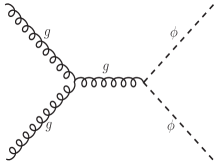
((a)) (a)

((b)) (b)

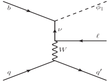
((c)) (c)

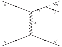
((d)) (d)

Figure 1: Sample Feynman diagrams for LQ production at the LHC. Diagrams (a) and (b) show pair production processes and (c) and (d) are examples of single productions.

II leptoquark models

Electromagnetic charge conservation forces the LQs that decay to a top quark and a charged lepton to have electromagnetic charge $\pm 1/3$ or $\pm 5/3$. From the classification of possible LQ states in Refs. Buchmuller:1986zs ; Dorsner:2016wpm , we see that only $S_{1}$, $R_{2}$ and $S_{3}$ have the desired decay modes, $\ell_{q}\to t\ell$ (where $\ell=\{e,\mu\}$). Below, we show these three types of LQs Lagrangians following the notations of Ref. Dorsner:2016wpm . To avoid proton decay constraints, we ignore the diquark operators.

II.1 Existing Models

$\blacksquare\quad$$S_{1}=(\overline{\mathbf{3}},\mathbf{1},1/3)$:
For $S_{1}$, one can write the following two renormalizable operators invariant under the SM gauge group ($G_{\mathrm{SM}}$):

$$\mathcal{L}\supset ~{}y^{LL}_{1\,ij}\bar{Q}_{L}^{C\,i}S_{1}i\tau^{2}L_{L}^{j}+y^{RR}_{1\,ij}\bar{u}_{R}^{C\,i}S_{1}e_{R}^{j}+\textrm{h.c.},$$ (1)

where $Q_{L}$ and $L_{L}$ are the SM left-handed quark and lepton doublets, respectively. The superscript $C$ denotes charge conjugation. The Pauli matrices are represented by $\tau^{k}$ with $k=\{1,~{}2,~{}3\}$. Here, the generation indices are denoted by $i,j=\{1,\ 2,\ 3\}$. This can be written explicitly as,

$$\mathcal{L}\supset -(y^{LL}_{1}U)_{ij}\bar{d}_{L}^{C\,i}S_{1}\nu_{L}^{j}+(V^{T}y^{LL}_{1})_{ij}\bar{u}_{L}^{C\,i}S_{1}e_{L}^{j}$$

$$+y^{RR}_{1\,ij}\bar{u}_{R}^{C\,i}S_{1}e_{R}^{j}+\textrm{h.c.}.$$ (2)

where $U$ and $V$ represent the Pontecorvo-Maki-Nakagawa-Sakata (PMNS) neutrino mixing matrix and the Cabibbo-Kobayashi-Maskawa (CKM) quark mixing matrix, respectively. Since the neutrino flavours cannot be distinguished at the LHC, we denote them by just $\nu$. Similarly, for LHC phenomenology in general, and in particular for our analysis, the small off-diagonal terms of the CKM matrix play negligible role. Hence, we assume a diagonal CKM matrix for simplicity. We identify the terms relevant for our analysis,

$$\mathcal{L}\supset \ y^{LL}_{1\ 3j}\left(-\bar{b}_{L}^{C}\nu_{L}+\bar{t}_{L}^{C}\ell_{L}^{j}\right)S_{1}+y^{RR}_{1\,3j}\ \bar{t}_{R}^{C}\ell_{R}^{j}S_{1}+\textrm{h.c.},$$ (3)

where $j=\{1,\ 2\}$.

$\blacksquare\quad$$S_{3}=(\overline{\mathbf{3}},\mathbf{3},1/3)$:
There is only one type of $G_{\mathrm{SM}}$-invariant renormalizable operator one can write for $S_{3}$:

$$\mathcal{L}\supset ~{}y^{LL}_{3\,ij}\bar{Q}_{L}^{C\,i,a}\epsilon^{ab}(\tau^{k}S^{k}_{3})^{bc}L_{L}^{j,c}+\textrm{h.c.},$$ (4)

Here, the $\mathrm{SU}(2)$ indices are denoted by $a,b,c=\{1,\ 2\}$. Expanding this we get,

$$\mathcal{L}\supset -(y^{LL}_{3}U)_{ij}\bar{d}_{L}^{C\,i}S^{1/3}_{3}\nu_{L}^{j}-\sqrt{2}y^{LL}_{3\,ij}\bar{d}_{L}^{C\,i}S^{4/3}_{3}e_{L}^{j}$$

$$+\sqrt{2}(V^{T}y^{LL}_{3}U)_{ij}\bar{u}_{L}^{C\,i}S^{-2/3}_{3}\nu_{L}^{j}$$

$$-(V^{T}y^{LL}_{3})_{ij}\bar{u}_{L}^{C\,i}S^{1/3}_{3}e_{L}^{j}+\textrm{h.c.},$$ (5)

The relevant interaction terms can be written as,

$$\mathcal{L}\supset -y^{LL}_{3\ 3j}\left[\left(\bar{b}_{L}^{C}\nu_{L}+\bar{t}_{L}^{C}\ell_{L}^{j}\right)S^{1/3}+\sqrt{2}\left(\bar{b}_{L}^{C}\ell_{L}^{j}S^{4/3}_{3}\right.\right.$$

$$-\left.\left.\bar{t}_{L}^{C}\nu_{L}S^{-2/3}\right)\right]+\textrm{h.c.},$$ (6)

with $j=\{1,\ 2\}$.

$\blacksquare\quad$$R_{2}=(\mathbf{3},\mathbf{2},7/6)$:
Similarly, for $R_{2}$ we have the following terms,

$$\mathcal{L} \supset -y^{RL}_{2\,ij}\bar{u}_{R}^{i}R_{2}^{a}\epsilon^{ab}L_{L}^{j,b}+y^{LR}_{2\,ji}\bar{e}_{R}^{j}R_{2}^{a\,*}Q_{L}^{i,a}+\textrm{h.c.},\$$

which, after expansion, can be written as,

$$\mathcal{L} \supset -y^{RL}_{2\ ij}\bar{u}^{i}_{R}e^{j}_{L}R_{2}^{5/3}+(y^{RL}_{2}U)_{ij}\bar{u}^{i}_{R}\nu^{j}_{L}R_{2}^{2/3}$$ (7)

$$+(y^{LR}_{2}V^{\dagger})_{ji}\bar{e}^{j}_{R}u^{i}_{L}R_{2}^{5/3\,*}+y^{LR}_{2\,ji}\bar{e}^{j}_{R}d^{i}_{L}R_{2}^{2/3\,*}+\textrm{~{}h.c.}.\;\;$$

We identify the terms relevant for us as,

$$\mathcal{L} \supset -y^{RL}_{2\ 3j}\ \bar{t}_{R}\ell^{j}_{L}R_{2}^{5/3}+y^{RL}_{2\ 3j}\ \bar{t}_{R}\nu_{L}R_{2}^{2/3}$$ (8)

$$+y^{LR}_{2\ j3}\ \bar{\ell}^{j}_{R}t_{L}R_{2}^{5/3\,*}+y^{LR}_{2\ j3}\ \bar{\ell}^{j}_{R}b_{L}R_{2}^{2/3\,*}+\textrm{h.c.},$$

with $j=\{1,\ 2\}$.

II.2 Simplified Models and Benchmark Scenarios

		Simplified model [Eqs. (9) – (10)]			LQ models [Eqs. (3) – (8)]
Benchmark scenario	Possible charge(s)	Type of LQ	Non-zero couplings equal to $\lambda$	Lepton chirality fraction	Type of LQ	Non-zero coupling equal to $\lambda$	Decay mode(s)	Branching ratio(s)
LCSS	$1/3$	$\phi_{1}$	$\lambda_{\ell}=\lambda_{\nu}$	$\eta_{L}=1$, $\eta_{R}=0$	$S_{3}^{1/3}$	$-y^{LL}_{3\ 3j}$	{$t\ell$, $b\nu$}	{$50\%$, $50\%$}
LCOS	$1/3$	$\phi_{1}$	$\lambda_{\ell}=-\lambda_{\nu}$	$\eta_{L}=1$, $\eta_{R}=0$	$S_{1}$	$y_{1\ 3j}^{LL}$	{$t\ell$, $b\nu$}	{$50\%$, $50\%$}
RC	$\{1/3,5/3\}$	$\{\phi_{1},\phi_{5}\}$	$\{\tilde{\lambda}_{\ell},\lambda_{\ell}\}$	$\eta_{L}=0$, $\eta_{R}=1$	$\{S_{1}$, $R_{2}^{5/3}\}$	$\{y_{1\ 3j}^{RR}$, $y^{LR}_{2\ j3}\}$	$t\ell$	$100\%$
LC	$5/3$	$\phi_{5}$	$\tilde{\lambda}_{\ell}$	$\eta_{L}=1$, $\eta_{R}=0$	$R_{2}^{5/3}$	$-y^{RL}_{2\ 3j}$	$t\ell$	$100\%$

Table 1: Summary of the four benchmark scenarios considered. They are explained in Section II.2.

Following Ref. Mandal:2015vfa , we write a simplified phenomenological Lagrangian for the models above,

$$\mathcal{L} \supset \lambda_{\ell}\left(\sqrt{\eta_{L}}\bar{t}_{L}^{C}\ell_{L}+\sqrt{\eta_{R}}\bar{t}_{R}^{C}\ell_{R}\right)\phi_{1}+\lambda_{\nu}\bar{b}_{L}^{C}\nu_{L}\phi_{1}+\ \textrm{h.c.},\ \ \ \$$ (9)

$$\mathcal{L} \supset \tilde{\lambda}_{\ell}\left(\sqrt{\eta_{L}}\bar{t}_{R}\ell_{L}+\sqrt{\eta_{R}}\bar{t}_{L}\ell_{R}\right)\phi_{5}+\textrm{h.c.}.$$ (10)

In this notation, a charge $1/3$ ($5/3$) scalar LQ is generically represented by $\phi_{1}$ ($\phi_{5}$). Here, $\eta_{L}$ and $\eta_{R}=(1-\eta_{L})$ are the fractions of leptons coming from LQ decays that are left-handed and right-handed, respectively. The simplified Lagrangian does not include any charge $2/3$ or $4/3$ LQ as such LQs would not couple with just a top quark and a charged lepton simultaneously.

For our analysis, we consider four benchmark coupling scenarios.

1. Left-handed Couplings with Same Sign (LCSS): In this scenario, we set $\lambda_{\ell}=\lambda_{\nu}=\lambda$, $\tilde{\lambda}_{\ell}=0$ and $\eta_{R}=0$, i.e., we have a $\phi_{1}$ LQ that couples to the left-handed leptons. As a result, it couples to both $t\ell$ and $b\nu$ pairs with equal strength and hence decays to either of the pairs with about $50\%$ BRs. In this scenario, the $\phi_{1}$ behaves like the charge $1/3$ component of $S_{3}$ (with $-y^{LL}_{3\ 3j}=\lambda$).

2. Left-handed Couplings with Opposite Sign (LCOS): We set $\lambda_{\ell}=-\lambda_{\nu}=\lambda$, $\tilde{\lambda}_{\ell}=0$ and $\eta_{R}=0$. In this scenario too a $\phi_{1}$ LQ couples with the left-handed leptons equally but with opposite signs. However, since it couples to both $t\mu$ and $b\nu$ pairs with equal (absolute) strength, it still decays to either a $t\ell$ or a $b\nu$ pair with about $50\%$ BRs. In this scenario, it behaves like an $S_{1}$ with $y_{1\ 3j}^{LL}=\lambda$ and $y_{1\ 3j}^{RR}=0$.

3. Right-handed Coupling (RC): In this scenario, the LQ has no weak charge and couples with only right handed leptons. This scenario is common to both $\phi_{1}$ and $\phi_{5}$ as we do not use the charge of leptoquark in our analysis. Here, we set $\tilde{\lambda}_{\ell}=\lambda_{\ell}=\lambda$, $\lambda_{\nu}=0$ and $\eta_{L}=0$. It decays to a $t\ell$ pair with $100\%$ BR. In this scenario, the LQ is either of $S_{1}$ type with $y_{1\ 3j}^{LL}=0$ and $y_{1\ 3j}^{RR}=\lambda$ or it is $R_{2}^{5/3}$ with $y^{LR}_{2\ j3}=\lambda$.

4. Left-handed Coupling (LC): In this scenario the LQ couples with only left handed charged leptons. This scenario is exclusive to $\phi_{5}$. Here, we set $-y^{RL}_{2\ 3j}=\tilde{\lambda}_{\ell}=\lambda$, $\lambda_{\ell}=\lambda_{\nu}=0$ and $\eta_{R}=0$. It decays to a $t\ell$ pair with $100\%$ BR.

We have summarized these four scenarios in Table 1.

III LHC Phenomenology & Search Strategy

We have used various publicly available packages for our analysis. We implement the Lagrangian of Eqs. (9) and (10) in FeynRules Alloul:2013bka to create the UFO Degrande:2011ua model files. Both the signal and the background events are generated in the event generator MadGraph5 Alwall:2014hca at the leading order (LO). The higher-order corrections are included by multiplying appropriate QCD $K$-factors wherever available. We use NNPDF2.3LO Ball:2012cx parton distribution functions (PDFs) for event generation by setting default dynamical renormalization and factorization scales used in MadGraph5. Events are passed through Pythia6 Sjostrand:2006za to perform showering and hadronization and matched up to two additional jets using MLM matching scheme Mangano:2006rw ; Hoche:2006ph with virtuality-ordered Pythia showers to remove the double counting of the matrix element partons with parton showers. Detector effects are simulated using Delphes3 deFavereau:2013fsa with the default CMS card. Fatjets are reconstructed using the FastJet Cacciari:2011ma package by clustering Delphes tower objects. We employ Cambridge-Achen Dokshitzer:1997in algorithm with radius parameter $R=1.5$ for fatjet clustering. To reconstruct hadronic tops from fatjets, we use a popular top tagger, namely the HEPTopTagger Plehn:2010st .

III.1 Production at the LHC

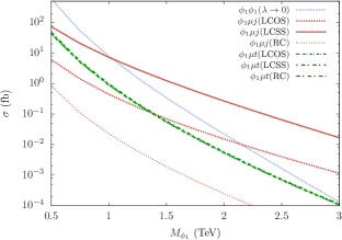
((a))    (a)

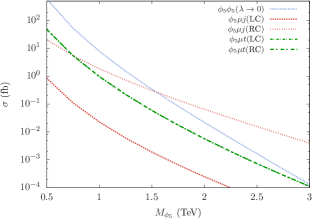
((b))    (b)

Figure 2: The parton-level cross sections of different production channels of $\phi_{1}$ and $\phi_{5}$ at the $14$ TeV LHC as functions of $M_{\phi}$. We display the muon channel cross sections; the electron channel have similar cross sections. The single production cross sections are computed for a benchmark coupling $\lambda=1$ (see Table 1). The pair production cross sections include an NLO QCD $K$-factor of 1.3 Mandal:2015lca . Here, the $j$ in the single production processes includes all the light jets as well as $b$-jets. Their cross sections are generated with a cut on the transverse momentum of the jet, $p^{j}_{\rm T}>20$ GeV.

As indicated in the introduction section, LQs are produced resonantly at the LHC through pair and single production channels. The pair production is mostly model independent [depends only on the universal QCD coupling, see e.g. Fig. 1(a)] and proceeds through the $gg$ and $qq$ initiated processes. In the LCOS and the LCSS models, the process $bb\to\phi_{1}\phi_{1}$ through the $t$-channel neutrino exchange is dependent on model coupling $\lambda$ [see Fig. 1(b)]. However, this contribution is small in the total pair production cross section. The pair production process leads to the following final state,

$$pp\to\phi\phi\to(t\ell)(t\ell)$$ (11)

where a $\phi$ stands for either a $\phi_{1}$ or a $\phi_{5}$. Single production channels, where a LQ is produced in association with a lepton and either a jet or a top-quark, are given as,

$$\left.\begin{array}[]{lcccl}pp&\to&\phi t\ell&\to&(t\ell)t\ell\\ pp&\to&\phi\ell j&\to&(t\ell)\ell j\end{array}\right\}.$$ (14)

In Fig. 2, we show the parton level cross sections of different production processes of $\phi_{1}$ [Fig. 2(a)] and $\phi_{5}$ [Fig. 2(b)]. The single productions are computed for $\lambda=1$. We see that for $\phi_{1}$, the single production processes depend heavily on whether it is an $S_{1}$ with LCOS/RC type couplings or an $S_{3}$ with LCSS coupling. In the LCSS scenario, the $pp\to\phi_{1}\ell j$ becomes the dominant process beyond $M_{\phi}\gtrsim 1$ TeV whereas in the LCOS scenario, it overtakes the pair production only for $M_{\phi}>2.2$ TeV. This difference happens since in the LCOS scenario, some single production diagrams [see e.g. Figs. 1(c) & 1(d)] interfere destructively because of the opposite relative sign of the $\lambda_{\ell}$ and $\lambda_{\nu}$ couplings, whereas in case of LCSS, they interfere constructively. In the RC scenario, $\phi_{1}$ does not couple to a $b$-quark or a left handed top quark (that can be produced from a $W$ boson and a $b$-quark interaction) and hence we do not expect $\sigma(pp\to\phi_{1}\ell j)$ to be large. We see that $\sigma(pp\to\phi_{1}\ell j)<\sigma(pp\to\phi_{1}\phi_{1})$ for $M_{\phi_{1}}<3$ TeV in this scenario. For $\phi_{5}$, the cross section of $pp\to\phi_{5}\ell j$ processes in the LC scenario is smaller than that in the RC scenario, as $\phi_{5}$ couples exclusively to a right handed top quark in this case.

It is clear from the cross section plots that for order one $\lambda$, it is important to consider single productions while estimating the discovery prospects. Before we move on, we note that the cross section plots do not show the full picture, as one has to consider the branching ratios and the detector effects. In the LCOS and LCSS scenarios, BR$(\phi\to t\ell)\sim 50\%$ whereas it is $100\%$ in the RC and LC scenarios.

III.2 Signal Topology

In our analysis, we only consider the hadronic decays of tops to reconstruct them in the final states. The characteristic of our signal is the presence of one or two boosted top quarks forming one/two top-like fatjets and two high-$p_{\rm T}$ leptons. From Eqs. (11) and (14), we see that if we define our signal as events containing exactly two high-$p_{\rm T}$ same flavour opposite sign (SFOS) leptons and at least one hadronic top-like fatjet in the final state then it would include both single and pair productions and enhance the sensitivity.

There is some overlap between the pair and the single production processes. For example, at the parton level, a $t\ell\,t\ell$ final state can be produced from both the pair production process as well as the $pp\to\phi t\ell$ processes. Hence one has to be careful to avoid double counting while computing single productions Mandal:2015vfa . In our simulations we achieve this by ensuring that for any single production process both $\phi$ and $\phi^{\dagger}$ are never on-shell simultaneously.

Background		$\sigma$	QCD
processes		(pb)	Order
$V+jets$	$Z+jets$	$6.33\times 10^{4}$	NNLO
Catani:2009sm ; Balossini:2009sa	$W+jets$	$1.95\times 10^{5}$	NLO
$VV+jets$	$WW+jets$	112.64	NLO
Campbell:2011bn	$WZ+jets$	46.74	NLO
	$ZZ+jets$	15.99	NLO
Single $t$	$tW$	70.0	N2LO
Kidonakis:2015nna	$tb$	218.0	N2LO
	$tj$	11.17	N2LO
$tt$ Muselli:2015kba	$tt+jets$	835.61	N3LO
$ttV$ Kulesza:2018tqz	$ttZ$	1.045	NLO+NNLL
	$ttW$	0.653	NLO+NNLL

Table 2: Total cross sections for the background processes considered in our analyses.We use these cross sections to obtain the higher order $K$-factors.

III.3 The SM Backgrounds

The main SM background processes for this signal topology would be those which give two high-$p_{\rm T}$ leptons and a top-like jet originating from an actual top quark or other jets (which can come from hadronic decays of the SM particles or from QCD jets). We see that the single $Z$ and $tt$ processes contribute dominantly. Processes with large cross section containing single lepton can also act as a background if the second lepton appear due to a jet misidentified as a lepton. However, due to very small misidentification rate, these class of processes contribute negligibly to the total background.

Although some backgrounds are seemingly huge (see Table 2), events that would satisfy the final signal selection criterion used in our analysis would actually come from a very specific kinematic region. With this in mind, we generate the background processes with some strong generation level cuts, for better statistics and saving computation time,

Generation level cuts:

1. $p_{\rm T}(\ell_{1})>250$ GeV,

2. the invariant mass of the lepton pair $M(\ell_{1},\ell_{2})>115$ GeV (the $Z$-mass veto).

Here, $\ell_{1}$ and $\ell_{2}$ denote the leptons with the highest and the second highest $p_{\rm T}$, respectively. We discuss the different background processes in more detail below.

1. $V+jets$:
   Inclusive single vector boson ($V={Z,W}$) production processes in the SM have very large cross sections and therefore, can act as potential backgrounds for our signal even if the cut efficiencies are extremely small. There are two types of single vector boson processes that we consider as potential backgrounds.

   1. $Z/\gamma^{*}+jets$: This background is generated by simulating the process, $pp\rightarrow Z/\gamma^{*}+(0,1,2,3)$-$jets\to\ell\ell+jets$ matched up to three extra partons. Here, the two high-$p_{\rm T}$ leptons can arise from the leptonic decays of the $Z$-boson and a top-like fatjet can originate from the QCD jets. Since the invariant mass of the two leptons peaks at $Z$-mass, this background is controlled by the $Z$-mass veto.

   2. $W+jets$: This process also has huge cross section like the previous one, but it is a reducible background. We generate it by simulating the process, $pp\rightarrow W+(0,1,2,3)$-$jets\to\ell\nu+jets$ matched up to three extra partons. Requirement of a top-like jet can be fulfilled if the QCD jets mimic as a top-jet. However, as we demand the second lepton also to have high $p_{\rm T}$ where the lepton misidentification efficiency becomes small, we found this background to be negligible.

2. $VV+jets$:
   There are four types of diboson processes viz. $Z_{\ell}Z_{h}$, $W_{h}Z_{\ell}$, $W_{\ell}W_{\ell}$ and $Z_{\ell}H_{h}$ that can act as sources of two high-$p_{\rm T}$ leptons. The subscripts “$\ell$” and “$h$” represent leptonic and hadronic decay modes respectively. In these cases, the required top-like jet can arise from the hadronic decay products of bosons or from the QCD jets. Processes containing leptonically decaying $Z$ can be drastically reduced by applying $Z$ mass veto on the invariant mass of the lepton pair. We do not consider the case where one lepton come from the vector boson decays and the other appear due to jets misidentified as leptons. We generate matched event samples including up to two jets of these processes.

3. $tt+jets$:
   The SM top pair production at the LHC can provide us two high-$p_{\rm T}$ leptons when both the tops decay leptonically. Additionally, a top-like jet which arise from the QCD jets together with those two leptons can mimic our signal. We find that, like the $Z$ background, this contribution is also significant in our case. A priori, the $t_{\ell}t_{h}$ process where one top decays leptonically and the other hadronically can also contribute to the background. We generate this events by matching up to two additional jets.

4. $ttV$:
   The SM processes with a top pair associated with a vector boson can act as backgrounds for our signal. We consider the following four cases viz. $t_{\ell}t_{\ell}Z_{h}$, $t_{\ell}t_{\ell}W_{h}$, $t_{h}t_{h}Z_{\ell}$, $t_{h}t_{\ell}W_{\ell}$ depending on the decays of tops and vector bosons. We generate these event samples without adding extra jets in the final state.

5. tW:
   The SM $pp\to t_{\ell}W_{\ell}$ process contains two leptons in the final state and contribute to the background for our signal. We generate this process using matching by adding up to two extra jets.

In Table 2 we collect the total cross sections of the background processes computed at various orders of QCD available in the literature. From these we compute the $K$-factors and, as mentioned, scale the corresponding LO cross sections in our analysis.

III.4 Event selection

We apply the following sets of cuts on the signal and background events sequentially.

1. (a) At least one top-jet (obtained from HEPTopTagger) with $p_{\rm T}(t_{h})>135$ GeV.

   (b) Two SFOS leptons with $p_{\rm T}(\ell_{1})>400$ GeV and $p_{\rm T}(\ell_{2})>200$ GeV and pseudorapidity $|\eta(\ell)|<2.5$. For electron we consider the barrel-endcap cut on $\eta$ between $1.37$ and $1.52$.

   (c) Invariant mass of lepton pair $M(\ell_{1},\ell_{2})>120$ GeV to avoid $Z$-peak.

   (d) The missing energy $\not{E}_{T}<200$ GeV.

2. The scalar sum of the transverse $p_{T}$ of all visible objects, $S_{T}>1.2\times{\rm Min}\left(M_{\phi},1750\right)$ GeV.

3. $M(\ell_{1},t)~{}\mathrm{OR}~{}M(\ell_{2},t)>0.8\times{\rm Min}\left(M_{\phi},1750\right)$ GeV.

In Fig. 3 we show the final signal selection efficiencies ($\varepsilon$) for different coupling hypotheses. We define $\varepsilon$ as,

$$\varepsilon=\frac{\mbox{Number of events surviving }\mathcal{C}_{1}+\mathcal{C}_{2}+\mathcal{C}_{3}}{\mbox{Number of events generated}}.$$ (15)

Since the $M_{\phi}$ dependent cuts (i.e., $\mathcal{C}_{2}$ and $\mathcal{C}_{3}$) get frozen beyond $M_{\phi}=1750$ GeV, we see the kink-like shapes at $1750$ GeV.

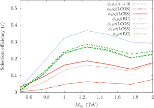
Figure 3: Final signal selection efficiencies ($\varepsilon$, see Eq. (15)) for different coupling configurations in the $\mu$-channel. Since for $M_{\phi}\geq 1.75$ TeV, the selection cuts do not change (see Section III.4) we display the efficiencies only up to $M_{\phi}=2$ TeV. The $e$-channel efficiencies are very much similar to these.

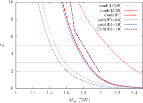
((a))    (a)

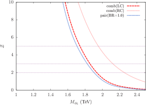
((b))    (b)

Figure 4: Expected significance ($\mathcal{Z}$) for observing the (a) $\phi_{1}$ and (b) $\phi_{2}$ signals over the SM backgrounds as functions of their masses for 3 ab^-1 of integrated luminosity at the 14TeV LHC for different coupling scenarios in the muon mode. The electron mode numbers can be seen from Table 3. We use the combined pair and single productions for the signals in the LCOS, LCSS, RC and LC scenarios. For comparison, we also show the pair production only significance for 50% and 100% BRs in the $\phi\to t\mu$ decay mode and the CMS statistical-uncertainty-only estimation for discovering $\phi_{1}$ CMS:2018yke . We have set $\lambda=1$ while computing the combined signals. Our estimations are obtained using the event selection cuts defined in Section III.4, i.e., only events with at least one hadronically decaying boosted top and two high-$p_{T}$ opposite sign electrons are considered.

Significance $\mathcal{Z}$	Limit on $M_{\phi}$ (TeV)
	The $\mu$ channel								The $e$ channel
	$\phi_{1}$					$\phi_{5}$			$\phi_{1}$					$\phi_{5}$
	Combined			Pair		Combined		Pair	Combined			Pair		Combined		Pair
	LCOS	LCSS	RC	BR=$0.5$	BR=$1.0$	LC	RC	BR=$1.0$	LCOS	LCSS	RC	BR=$0.5$	BR=$1.0$	LC	RC	BR=$1.0$
5	1.47	2.08	1.73	1.42	1.71	1.74	1.96	1.71	1.45	2.11	1.72	1.39	1.70	1.74	1.97	1.70
3	1.59	2.29	1.84	1.52	1.83	1.86	2.12	1.83	1.58	2.33	1.84	1.52	1.83	1.86	2.16	1.83
2	1.69	2.44	1.92	1.61	1.90	1.94	2.25	1.90	1.69	2.50	1.93	1.62	1.91	1.95	2.30	1.91

Table 3: The mass limits corresponding to $5\sigma$ (discovery), $3\sigma$ and $2\sigma$ (exclusion) significances ($\mathcal{Z}$) for observing the (a) $\phi_{1}$ and (b) $\phi_{2}$ signals over the SM backgrounds for 3 ab^-1 integrated luminosity at the 14TeV LHC with combined and pair only signals. The $\mu$-channel numbers can also be seen from Fig. 4.

IV Discovery potential

With the number of signal ($N_{S}$) and background ($N_{B}$) events surviving the selection cuts defined in Section III.4, we estimate the expected significance ($\mathcal{Z}$) using the following formula:

$$\mathcal{Z}=\sqrt{2\left(N_{S}+N_{B}\right)\ln\left(\frac{N_{S}+N_{B}}{N_{B}}\right)-2N_{S}}\,.$$ (16)

In Fig. 4, we show the expected significances for observing the $\phi_{1}$ and $\phi_{2}$ signals in the benchmark coupling scenarios (Section II.2) over the SM backgrounds in the muon mode as functions of their masses for 3 ab^-1 of integrated luminosity at the 14 TeV LHC. As explained, we have used the combined signal (i.e. pair and single production events together) to estimate the significances in the LCOS, LCSS, RC and LC scenarios with $\lambda=1$. For the LCOS and LCSS scenarios, the BR of LQ to $te$ mode is 50% whereas for the RC and LC scenarios it is 100%. For comparison, we also show the expected significance for only the pair production (i.e. $\lambda\to 0$) with 50% and 100% BR cases. In Table 3 we explicitly show the mass values corresponding to $5\sigma$ (discovery), $3\sigma$ and $2\sigma$ (exclusion) significances for different coupling hypotheses in both $e$ and $\mu$ channels.

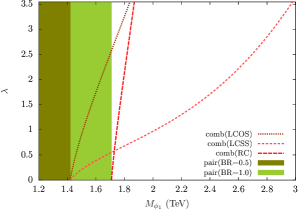
((a))    (a)

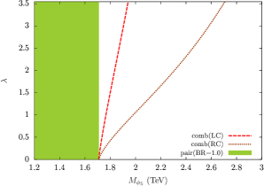
((b))    (b)

Figure 5: The $5\sigma$ discovery reaches in the $\lambda-M_{\phi}$ planes – (a) for a charge $1/3$ scalar LQ and (b) for a charge $5/3$ scalar LQ. These plots show the lowest $\lambda$ needed to observe $\phi_{1}$ and $\phi_{5}$ signals with $5\sigma$ significance for a range of $M_{\phi}$ with 3 ab^-1 of integrated luminosity. The pair production only regions for 50% and 100% BRs in the $\phi\to t\mu$ decay mode are shown with shades of green. Since the pair production is insensitive to $\lambda$, a small coupling is sufficient to attain $5\sigma$ significance within the green regions.

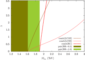
((a))    (a)

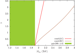
((b))    (b)

Figure 6: The $2\sigma$ exclusion limits in the $\lambda-M_{\phi}$ planes – (a) for a charge $1/3$ scalar LQ and (b) for a charge $5/3$ scalar LQ. These plots show the lowest $\lambda$ that can be excluded by the HL-LHC with 3 ab^-1 of integrated luminosity. The pair production only regions for 50% and 100% BRs in the $\phi\to t\mu$ decay mode are shown with green shades.

As already mentioned, the CMS collaboration has projected the expected significance for scalar LQs decaying into $t\mu$ pairs in the pair production channel at the $14$ TeV HL-LHC CMS:2018yke . There, with $100$% BR in the $t\mu$ mode, the $5\sigma$ discovery reach goes to about $1.8$ TeV (considering statistical uncertainty only). Our estimate is quite close, $\sim 1.7$ TeV if we consider only pair production with 100% BR in the $\phi_{1}\to t\mu$ decay mode (see Table. 3). This reach can decrease to $1.4$ TeV if the BR falls by $50$%. However, if we include single productions, the $5\sigma$ reach goes up to $2.1$ TeV in the LCSS scenario (where the $\phi_{1}$ behaves like the charge $1/3$ component of $S_{3}$). This drastic enhancement of $700$ GeV in the discovery reach happens because of the (relatively) large $pp\to\phi_{1}\ell j$ cross section in the high mass region leading to a substantial number of events surviving the applied selection cuts. However, in the LCOS scenario where a $\phi_{1}$ behaves like an $S_{1}$, this increment is minor, just about $50$ GeV, as destructive interference reduces the single production cross sections.

In the RC scenario, the total single production cross section of $\phi_{1}$ is small compared to the pair production one. Hence, the discovery reach is almost identical to that in the pair production only case. A similar situation is observed in the LC scenario for $\phi_{5}$. As explained in Section III, in both the RC scenario for $\phi_{1}$ and the LC scenario for $\phi_{5}$, leptoquarks couple to the right-handed tops. As a result, single productions in these cases have small cross sections as right-handed tops can couple to the charged current only via chirality flipping.

For any $M_{\phi}$ our signal cross section depends on $\lambda$ as,

$$\sigma_{\rm signal}\approx\sigma_{\rm pair}(M_{\phi})+\lambda^{2}\sigma_{\rm single}(\lambda=1,M_{\phi}),$$ (17)

i.e., for any $M_{\phi}$ if $\lambda$ increases the signal increases. Using this relation one can recast the plots in Fig. 4 in the $\lambda-M_{\phi}$ plane, as we have done in Fig. 5. These plots show the lowest $\lambda$ needed to observe $\phi_{1}$ and $\phi_{5}$ signals with $5\sigma$ significance for a range of $M_{\phi}$ with 3 ab^-1 of integrated luminosity. For all the points below a curve, the expected significance would be less than $5\sigma$. In Fig. 6 we show the corresponding plots for $2\sigma$ significance. In other words, these plot give us the lowest couplings that can be excluded at the HL-LHC.

V Summary and conclusions

In this paper, we have studied the HL-LHC reach for discovering scalar LQs that decay to a top quark and a charged lepton. In particular, we have focused on charge 1/3 ($\phi_{1}$) and 5/3 ($\phi_{5}$) scalar LQs that produce a resonance system with hadronically decaying boosted top quark and an electron or a muon. According to the classification given in Refs. Buchmuller:1986zs ; Dorsner:2016wpm , only $S_{1}$, $S_{3}$ (charge 1/3 component of the triplet) and $R_{2}$ (charge 5/3 component of the doublet) scalar LQs can produce the specific signatures we consider. We have also introduced a simplified Lagrangian for $\phi=\{\phi_{1},\phi_{5}\}$ suitable for bottom-up searches. We have shown how these simplified models connect to the actual models for different coupling configurations.

LQs can be produced in pairs or singly ($pp\to\phi\ell j,\phi\ell t$) at the LHC. When a LQ couples mostly with the third generation quarks, usually the pair production channels are considered for their discovery assuming the single productions to be suppressed because of small $b$-PDF. Interestingly, we find that for order one couplings, cross section of some single production channels can be larger than the pair production cross section. Hence, it is natural to expect that the inclusion of these single production channels would, therefore, increase their discovery prospects beyond the pair production searches. However, this depends on the underlying model; the $pp\to\phi_{1}\ell j$ single production cross sections can differ drastically depending on the representation in which $\phi_{1}$ belongs to. In particular, for the charge $1/3$ component of $S_{3}$ (the LCSS scenario, see Section II.2), $pp\to\phi\ell j$ has larger cross section than the pair production in the heavier mass region. This also happens for $R_{2}^{5/3}$ (with $y^{LR}$ type coupling the RC scenario). However, for $S_{1}$ (the LCOS scenario), the single productions have smaller cross sections because of destructive interference between certain diagrams [which is caused by the opposite signs of the left handed charged lepton and neutrino couplings, see Eq. (9)].

We have proposed a selection criterion that would retain events from both pair and single production processes so that the search becomes a combined one with increased reach. Our signal topology is defined by at least one hadronically decaying boosted top and two opposite sign same flavour leptons. With this, we have found that the $5\sigma$ discovery reach for $\phi_{1}$ in LCSS scenario with $\lambda=1$ is about 2.1 TeV at the 14 TeV LHC with 3 ab^-1 integrated luminosity. In the LCSS scenario, the BR $\phi\to t\ell$ mode is 50% and the reach for the pair production is only about 1.4 TeV. This significant improvement is due to constructive interference among certain single production diagrams. This increases the $pp\to\phi\ell j$ cross section about one order in magnitude compared to the LCOS case where destructive interference makes single production less important. Finally we note that the enhancements of discovery reach due to the single production channels would increase further if the new couplings are more than one as the single production cross sections scale as square of the coupling involved.

- (1) BaBar collaboration, J. P. Lees et al., Evidence for an excess of decays, Phys. Rev. Lett. 109 (2012) 101802, [1205.5442].
- (2) BaBar collaboration, J. P. Lees et al., Measurement of an Excess of Decays and Implications for Charged Higgs Bosons, Phys. Rev. D88 (2013) 072012, [1303.0571].
- (3) LHCb collaboration, R. Aaij et al., Measurement of the ratio of branching fractions , Phys. Rev. Lett. 115 (2015) 111803, [1506.08614]. [Erratum: Phys. Rev. Lett.115,no.15,159901(2015)].
- (4) LHCb collaboration, R. Aaij et al., Measurement of the ratio of the and branching fractions using three-prong -lepton decays, Phys. Rev. Lett. 120 (2018) 171802, [1708.08856].
- (5) LHCb collaboration, R. Aaij et al., Test of Lepton Flavor Universality by the measurement of the branching fraction using three-prong decays, Phys. Rev. D97 (2018) 072013, [1711.02505].
- (6) Belle collaboration, S. Hirose et al., Measurement of the lepton polarization and in the decay , Phys. Rev. Lett. 118 (2017) 211801, [1612.00529].
- (7) Belle collaboration, S. Hirose et al., Measurement of the lepton polarization and in the decay with one-prong hadronic decays at Belle, Phys. Rev. D97 (2018) 012004, [1709.00129].
- (8) Belle collaboration, A. Abdesselam et al., Measurement of and with a semileptonic tagging method, 1904.08794.
- (9) HFLAV collaboration, Y. Amhis et al., Averages of -hadron, -hadron, and -lepton properties as of summer 2016, Eur. Phys. J. C77 (2017) 895, [1612.07233]. We have used the Spring 2019 averages from https://hflav-eos.web.cern.ch/hflav-eos/semi/spring19/html/RDsDsstar/RDRDs.html. For regular updates see https://hflav.web.cern.ch/content/semileptonic-b-decays.
- (10) D. Bigi and P. Gambino, Revisiting , Phys. Rev. D94 (2016) 094008, [1606.08030].
- (11) F. U. Bernlochner, Z. Ligeti, M. Papucci and D. J. Robinson, Combined analysis of semileptonic decays to and : , , and new physics, Phys. Rev. D95 (2017) 115008, [1703.05330]. [erratum: Phys. Rev.D97,no.5,059902(2018)].
- (12) D. Bigi, P. Gambino and S. Schacht, , , and the Heavy Quark Symmetry relations between form factors, JHEP 11 (2017) 061, [1707.09509].
- (13) S. Jaiswal, S. Nandi and S. K. Patra, Extraction of from and the Standard Model predictions of , JHEP 12 (2017) 060, [1707.09977].
- (14) G. Hiller and F. Kruger, More model-independent analysis of processes, Phys. Rev. D69 (2004) 074020, [hep-ph/0310219].
- (15) M. Bordone, G. Isidori and A. Pattori, On the Standard Model predictions for and , Eur. Phys. J. C76 (2016) 440, [1605.07633].
- (16) LHCb collaboration, R. Aaij et al., Test of lepton universality using decays, Phys. Rev. Lett. 113 (2014) 151601, [1406.6482].
- (17) LHCb collaboration, R. Aaij et al., Differential branching fractions and isospin asymmetries of decays, JHEP 06 (2014) 133, [1403.8044].
- (18) LHCb collaboration, R. Aaij et al., Angular analysis of the decay using 3 fb-1 of integrated luminosity, JHEP 02 (2016) 104, [1512.04442].
- (19) LHCb collaboration, R. Aaij et al., Test of lepton universality with decays, JHEP 08 (2017) 055, [1705.05802].
- (20) LHCb collaboration, R. Aaij et al., Search for lepton-universality violation in decays, Phys. Rev. Lett. 122 (2019) 191801, [1903.09252].
- (21) J. C. Pati and A. Salam, Lepton Number as the Fourth Color, Phys. Rev. D10 (1974) 275–289. [Erratum: Phys. Rev.D11,703(1975)].
- (22) H. Georgi and S. L. Glashow, Unity of All Elementary Particle Forces, Phys. Rev. Lett. 32 (1974) 438–441.
- (23) B. Schrempp and F. Schrempp, Light Leptoquarks, Phys. Lett. B153 (1985) 101–107.
- (24) R. Barbier et al., R-parity violating supersymmetry, Phys. Rept. 420 (2005) 1–202, [hep-ph/0406039].
- (25) M. Kohda, H. Sugiyama and K. Tsumura, Lepton number violation at the LHC with leptoquark and diquark, Phys. Lett. B718 (2013) 1436–1440, [1210.5622].
- (26) B. Gripaios, A. Papaefstathiou, K. Sakurai and B. Webber, Searching for third-generation composite leptoquarks at the LHC, JHEP 01 (2011) 156, [1010.3962].
- (27) J. M. Arnold, B. Fornal and M. B. Wise, Phenomenology of scalar leptoquarks, Phys. Rev. D88 (2013) 035009, [1304.6119].
- (28) P. Bandyopadhyay and R. Mandal, Revisiting scalar leptoquark at the LHC, Eur. Phys. J. C78 (2018) 491, [1801.04253].
- (29) N. Vignaroli, Seeking leptoquarks in the plus missing energy channel at the high-luminosity LHC, Phys. Rev. D99 (2019) 035021, [1808.10309].
- (30) T. Mandal, S. Mitra and S. Raz, motivated leptoquark scenarios: Impact of interference on the exclusion limits from LHC data, Phys. Rev. D99 (2019) 055028, [1811.03561].
- (31) J. Roy, Probing leptoquark chirality via top polarization at the Colliders, 1811.12058.
- (32) A. Alves, O. J. P. Éboli, G. Grilli Di Cortona and R. R. Moreira, Indirect and monojet constraints on scalar leptoquarks, Phys. Rev. D99 (2019) 095005, [1812.08632].
- (33) U. Aydemir, T. Mandal and S. Mitra, Addressing the anomalies with an leptoquark from grand unification, 1902.08108.
- (34) CMS collaboration, A. M. Sirunyan et al., Search for third-generation scalar leptoquarks decaying to a top quark and a lepton at 13 TeV, Eur. Phys. J. C78 (2018) 707, [1803.02864].
- (35) CMS collaboration, A. M. Sirunyan et al., Constraints on models of scalar and vector leptoquarks decaying to a quark and a neutrino at 13 TeV, Phys. Rev. D98 (2018) 032005, [1805.10228].
- (36) ATLAS collaboration, M. Aaboud et al., Searches for scalar leptoquarks and differential cross-section measurements in dilepton-dijet events in proton-proton collisions at a centre-of-mass energy of = 13 TeV with the ATLAS experiment, Eur. Phys. J. C79 (2019) 733, [1902.00377].
- (37) ATLAS collaboration, M. Aaboud et al., Searches for third-generation scalar leptoquarks in = 13 TeV pp collisions with the ATLAS detector, JHEP 06 (2019) 144, [1902.08103].
- (38) B. Diaz, M. Schmaltz and Y.-M. Zhong, The leptoquark Hunter’s guide: Pair production, JHEP 10 (2017) 097, [1706.05033].
- (39) M. Schmaltz and Y.-M. Zhong, The leptoquark Hunter’s guide: large coupling, JHEP 01 (2019) 132, [1810.10017].
- (40) CMS collaboration, A. M. Sirunyan et al., Search for leptoquarks coupled to third-generation quarks in proton-proton collisions at 13 TeV, Phys. Rev. Lett. 121 (2018) 241802, [1809.05558].
- (41) CMS collaboration, Projection of searches for pair production of scalar leptoquarks decaying to a top quark and a charged lepton at the HL-LHC, Tech. Rep. CMS-PAS-FTR-18-008, 2018.
- (42) T. Mandal and S. Mitra, Probing Color Octet Electrons at the LHC, Phys. Rev. D87 (2013) 095008, [1211.6394].
- (43) T. Mandal, S. Mitra and S. Seth, Single Productions of Colored Particles at the LHC: An Example with Scalar Leptoquarks, JHEP 07 (2015) 028, [1503.04689].
- (44) T. Mandal, S. Mitra and S. Seth, Probing Compositeness with the CMS & Data, Phys. Lett. B758 (2016) 219–225, [1602.01273].
- (45) W. Buchmuller, R. Ruckl and D. Wyler, Leptoquarks in Lepton - Quark Collisions, Phys. Lett. B191 (1987) 442–448. [Erratum: Phys. Lett.B448,320(1999)].
- (46) I. Dors̆ner, S. Fajfer, A. Greljo, J. F. Kamenik and N. Kos̆nik, Physics of leptoquarks in precision experiments and at particle colliders, Phys. Rept. 641 (2016) 1–68, [1603.04993].
- (47) A. Alloul, N. D. Christensen, C. Degrande, C. Duhr and B. Fuks, FeynRules 2.0 - A complete toolbox for tree-level phenomenology, Comput. Phys. Commun. 185 (2014) 2250–2300, [1310.1921].
- (48) C. Degrande, C. Duhr, B. Fuks, D. Grellscheid, O. Mattelaer and T. Reiter, UFO - The Universal FeynRules Output, Comput. Phys. Commun. 183 (2012) 1201–1214, [1108.2040].
- (49) J. Alwall, R. Frederix, S. Frixione, V. Hirschi, F. Maltoni, O. Mattelaer et al., The automated computation of tree-level and next-to-leading order differential cross sections, and their matching to parton shower simulations, JHEP 07 (2014) 079, [1405.0301].
- (50) R. D. Ball et al., Parton distributions with LHC data, Nucl. Phys. B867 (2013) 244–289, [1207.1303].
- (51) T. Sjostrand, S. Mrenna and P. Z. Skands, PYTHIA 6.4 Physics and Manual, JHEP 05 (2006) 026, [hep-ph/0603175].
- (52) M. L. Mangano, M. Moretti, F. Piccinini and M. Treccani, Matching matrix elements and shower evolution for top-quark production in hadronic collisions, JHEP 01 (2007) 013, [hep-ph/0611129].
- (53) S. Hoeche, F. Krauss, N. Lavesson, L. Lonnblad, M. Mangano, A. Schalicke et al., Matching parton showers and matrix elements, in HERA and the LHC: A Workshop on the implications of HERA for LHC physics: Proceedings Part A, 2006. hep-ph/0602031.
- (54) DELPHES 3 collaboration, J. de Favereau, C. Delaere, P. Demin, A. Giammanco, V. Lemaître, A. Mertens et al., DELPHES 3, A modular framework for fast simulation of a generic collider experiment, JHEP 02 (2014) 057, [1307.6346].
- (55) M. Cacciari, G. P. Salam and G. Soyez, FastJet User Manual, Eur. Phys. J. C72 (2012) 1896, [1111.6097].
- (56) Y. L. Dokshitzer, G. D. Leder, S. Moretti and B. R. Webber, Better jet clustering algorithms, JHEP 08 (1997) 001, [hep-ph/9707323].
- (57) T. Plehn, M. Spannowsky, M. Takeuchi and D. Zerwas, Stop Reconstruction with Tagged Tops, JHEP 10 (2010) 078, [1006.2833].
- (58) T. Mandal, S. Mitra and S. Seth, Pair Production of Scalar Leptoquarks at the LHC to NLO Parton Shower Accuracy, Phys. Rev. D93 (2016) 035018, [1506.07369].
- (59) S. Catani, L. Cieri, G. Ferrera, D. de Florian and M. Grazzini, Vector boson production at hadron colliders: a fully exclusive QCD calculation at NNLO, Phys. Rev. Lett. 103 (2009) 082001, [0903.2120].
- (60) G. Balossini, G. Montagna, C. M. Carloni Calame, M. Moretti, O. Nicrosini, F. Piccinini et al., Combination of electroweak and QCD corrections to single W production at the Fermilab Tevatron and the CERN LHC, JHEP 01 (2010) 013, [0907.0276].
- (61) J. M. Campbell, R. K. Ellis and C. Williams, Vector boson pair production at the LHC, JHEP 07 (2011) 018, [1105.0020].
- (62) N. Kidonakis, Theoretical results for electroweak-boson and single-top production, PoS DIS2015 (2015) 170, [1506.04072].
- (63) C. Muselli, M. Bonvini, S. Forte, S. Marzani and G. Ridolfi, Top Quark Pair Production beyond NNLO, JHEP 08 (2015) 076, [1505.02006].
- (64) A. Kulesza, L. Motyka, D. Schwartländer, T. Stebel and V. Theeuwes, Associated production of a top quark pair with a heavy electroweak gauge boson at NLONNLL accuracy, Eur. Phys. J. C79 (2019) 249, [1812.08622].