Equalization of pulse timings in an excitable microlaser system with delay

Abstract

An excitable semiconductor micropillar laser with delayed optical feedback is able to regenerate pulses by the excitable response of the laser. It has been shown that almost any pulse sequence can, in principle, be excited and regenerated by this system over short periods of time. We show experimentally and numerically that this is not true anymore in the long term: rather, the system settles down to a stable periodic orbit with equalized timing between pulses. Several such attracting periodic regimes with different numbers of equalized pulse timing may coexist and we study how they can be accessed with single external optical pulses of sufficient strength that need to be timed appropriately. Since the observed timing equalization and switching characteristics are generated by excitability in combination with delayed feedback, our results will be of relevance beyond the particular case of photonics, especially in neuroscience.

Excitability is observed in many natural and artificial systems, including spiking neurons, cardiac cells, and semiconductor lasers. It corresponds to the all-or-none response in the form of a single spike to an input external perturbation, depending on whether or not the amplitude of the perturbation exceeds the so-called excitable threshold (Izhikevich, 2007). When subject to delayed feedback, an excitable system can either remain in its quiet state for small external perturbations or, with an adequate control pulse of sufficient strength, it can then regenerate its own excitable response after the reinjection time $\tau$. This very general mechanism for self-pulsations has been implemented in different optical systems, including a coherently driven VCSEL (Garbin et al., 2015), a VCSEL subject to opto-electronic feedback (Marino and Giacomelli, 2017), coupled semiconductor lasers (Kelleher et al., 2010), a photonic resonator with optical self-feedback (Romeira et al., 2016) and a micropillar laser with integrated saturable absorber (Terrien et al., 2017a).

Since almost arbitrary pulse timing patterns can, in principle, be excited and regenerated after each delay, regenerative dynamics can be of particular interest for producing complex optically-controllable temporal pulsing patterns (Marconi et al., 2014; Jang et al., 2015; Camelin et al., 2016; Javaloyes et al., 2016; Terrien et al., 2018) or for spike-based optical memory applications (Garbin et al., 2015; Romeira et al., 2016; Shastri et al., 2016; Terrien et al., 2018). In the context of biological spiking neurons, delayed self-connections have also been recognized to play a central role in the persistent regeneration of input stimuli (Foss et al., 1996; Connors, 2002; Chaudhuri and Fiete, 2016). Systems with delay generally display rich dynamics with coexistence between different types of attractors (Ikeda et al., 1982; Yanchuk and Perlikowski, 2009). Consequently, it is an important question to determine the long-term dynamics of regenerative pulsing in excitable systems with delay.

Here we show experimentally and theoretically that it is not possible to regenerate arbitrary timing patterns in the long term: any triggered pulse pattern will equalize, upon sufficiently many successive regenerations, to an equidistant pulse train. Hence, positional information of non-equalized pulse patterns is preserved only for short periods of time and cannot be sustained in the long-term. Since the long-term information is encoded in the number of pulses in the feedback loop, we also investigate how one can switch between different equalized stable pulse trains. From a theoretical perspective, this is related to the structure of their basins of attraction, which we investigate numerically. The underlying physics of equalization as well as of switching between patterns is entirely the result of an interplay between the timescale of the slow dynamical variable (here the net gain dynamics (Nizette et al., 2006)) and the latency time of the excitable system (Selmi et al., 2016). As such, this mechanism is very general for excitable systems subject to delayed feedback.

In this Letter, we consider an excitable microlaser with integrated saturable absorber (Barbay et al., 2005; Elsass et al., 2010; Barbay et al., 2011; Selmi et al., 2014) and delayed optical feedback (Terrien et al., 2017a, 2018). Thanks to its small footprint, sub-nanosecond response time and easy bi-dimensional integration, this device is of particular interest for applications ranging from photonic spike processing (Nahmias et al., 2013; Prucnal et al., 2016) for efficient optical communications applications to ultrafast artificial neural networks. Without feedback, the solitary micropillar laser is excitable in a wide pump parameter region below the self-pulsing threshold (Barbay et al., 2011) and displays various neuromimetic properties such as a relative refractory period (Selmi et al., 2014), temporal summation (Selmi et al., 2015) and spike latency (Selmi et al., 2016; Erneux and Barbay, 2018). In the presence of delayed optical feedback, it sustains trains of regenerative optical pulses, which can be asymmetrically perturbed by noise (Terrien et al., 2017a) or added and erased by single optical perturbations (Terrien et al., 2018).

The experimental setup consists of a micropillar laser with two gain and one saturable absorber quantum wells, which emits light at a wavelength close to 980 nm. Part of the output light is sent back into the micropillar after a delay $\tau$, through free-space propagation and reflection by a mirror at several tens of cm from the laser. A beamsplitter in the optical feedback path (R/T=70/30) redirects some of the light to a fast avalanche photodetector or a camera. The micropillar is pumped at 800nm, and short optical perturbations of 80 ps duration can be sent by a mode-locked Ti:Sa laser emitting at the pump wavelength.

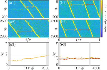
Figure 1: (a),(b): Experimental pulse trains following two (a) and three (b) perturbations, for a feedback delay of 8.2ns. Shown are the pseudo-space representation of the time traces observed shortly after the perturbations [(a1) and (b1)] and after several thousands of round trips [(a2) and (b2)]. The pulse-to-pulse timing $\Delta p$ (as shown by arrows in (a1) and (b1)) is plotted versus the round trip number in panels (a3) and (b3), where the shaded areas are the time segments represented in (a1–a2) and (b1–b2).

The experimental system is modeled accurately by the Yamada rate equations with incoherent delayed feedback (Yamada, 1993; Krauskopf and Walker, 2012; Barbay et al., 2011; Selmi et al., 2014; Terrien et al., 2017a, 2018) — a system of three DDEs for the dimensionless gain $G$, absorption $Q$ and intensity $I$:

$$\begin{split}\dot{G}&=\gamma_{G}(A-G-GI),\\ \dot{Q}&=\gamma_{Q}(B-Q-aQI),\\ \dot{I}&=(G-Q-1)I+\kappa I(t-\tau).\end{split}$$ (1)

Here, $A$ is the scaled pump parameter (relative to pump at transparency), $B$ is the non-saturable absorption, $a$ is the saturation parameter, and $\gamma_{G}$ and $\gamma_{Q}$ are the carrier recombination rates in the gain and absorber media, respectively. The optical feedback is described by the delayed term in the intensity equation, where $\kappa$ is the feedback strength and $\tau$ is the feedback delay. We consider here the same parameter values as in (Terrien et al., 2018): $A=2.4$, $B=2.2$, $\gamma_{G}=0.01$, $\gamma_{Q}=0.02$, $a=5$, $\kappa=0.05$, $\tau=1100$. These are chosen both to match the known physical parameters and the experimental observations. In particular, the small values of $\gamma_{G}$ and $\gamma_{Q}$ account for the slow non-radiative recombination of the carriers in the gain and absorber media, compared to the fast timescale of the laser field intensity.

Figure 1(a) and (b) show experimental results on the convergence of irregularly spaced pulse trains to regularly spaced ones following two and three external perturbations, respectively. In panels (a1)–(a2) and (b1)–(b2) the temporal traces are folded at approximately the delay $\tau$ and stacked vertically in a pseudo-space representation (Giacomelli and Politi, 1998). Initially non-equidistant pulse trains in the external cavity become equidistant after several thousands of round trips, as shown in panels (a2) and (b2). The slow convergence towards equidistant pulsing patterns is highlighted in panels (a3) and (b3), which represent the pulse-to-pulse timing $\Delta p$ versus the round trip number, from the instant when the pulse trains are triggered by external perturbations. The pulse-to-pulse timing $\Delta p$ slowly converges to a value close to a half or a third of the delay time $\tau$, respectively, as equidistant pulsing is approached. This slow convergence rate is of the order of a few ps per round trip, to be compared to the pulse duration of approximately 200 ps. It can be observed in the experiment only over long time periods. In contrast to the ultra weak soliton interaction observed in (Jang et al., 2013), it can be simply explained by the variation of the response latency time of the excitable microlaser in the slowly recovering landscape of the net gain dynamics (Dubbeldam et al., 1999; Selmi et al., 2016; Erneux and Barbay, 2018; Terrien et al., 2018). This response latency becomes identical only when all the re-injected pulses experience an identical net gain (Selmi et al., 2014; Terrien et al., 2018). This configuration corresponds to a stable equidistant pulse train in the case of a fast SA. The stochastic fluctuations of the pulse-to-pulse timing are explained by the presence of pump noise in the system, which induces stochastic fluctuations of the microlaser net gain (Terrien et al., 2017a).

The Yamada model with feedback (1) shows excellent agreement with these experimental observations. Its phase portraits are calculated with the continuation toolbox DDE-Biftool (Engelborghs et al., 2001; Sieber et al., 2015) and show a high degree of multistability. In particular, one stable equilibrium corresponding to the non-lasing solution coexists with six stable periodic solutions with different periods $T_{n}$ and equalized pulse timings, whose corresponding time series are represented in figure 2(a1)–(a6). Their periods are close to sub-multiples of the delay time $\tau$ (Terrien et al., 2017b), and they are hereafter referred to as 1-pulse solution, 2-pulse solution, and so on. A Floquet stability analysis has confirmed that the solutions with two to six coexisting pulses in the external cavity are only weakly stable (Terrien et al., 2018). Importantly, for the chosen parameters, no stable solution exists that corresponds to pulse trains with non-equidistant pulses. Therefore, all pulsing dynamics must converge towards one of the attracting periodic solution represented in Figure 2(a). As observed in the experiment, the convergence to the weakly stable pulsing regimes occurs on a slow timescale (Terrien et al., 2018) compared to the feedback delay time.

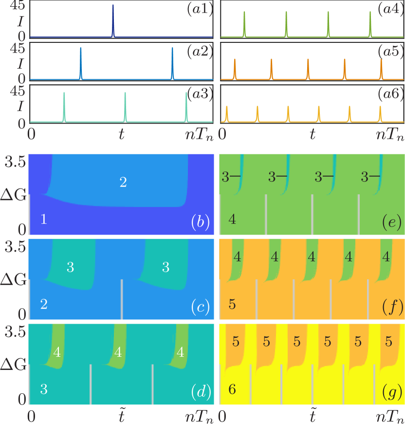
Figure 2: (a1)–(a6): Intensity time series of the stable periodic pulsing regimes of equations (1) represented over $n$ periods $T$, with $n$ the number of pulses in the span of the delay $\tau$. (b)–(g): Basins of attraction of (1) in the plane of timing $\tilde{t}$ and amplitude $\Delta G$ of a gain perturbation, when one (b) to six (g) equidistant pulses initially exist in the external cavity. The color represents the number of pulses observed in the long-term in the external cavity (see (a1)–(a6) for the color code), and the vertical gray lines indicate the timing of the pre-existing pulses.

The final state of a multistable system depends crucially on the initial conditions. For each attractor in figure 2(a), its basin of attraction is the set of initial conditions for which the system settles on that attractor after transient dynamics. From a practical point of view, the structure of these basins of attraction gives essential information on how to access the different coexisting stable pulsing regimes and, as such, on how to control the long-term dynamics of the multistable system (Pisarchik and Feudel, 2014). In systems of ordinary differential equations (ODEs) with up to three dimensions, the invariant manifolds that bound the different basins of attraction can be calculated with advanced numerical methods (Krauskopf et al., 2005). However, we deal here with a system of delay-differential equations (DDEs), whose phase space is intrinsically of infinite dimension (see e.g. (Balachandran et al., 2009)). The numerical continuation of the projections of such invariant manifolds is, hence, more complex (Krauskopf and Green, 2003; Keane and Krauskopf, 2018), and we rather integrate (1) numerically to map the basins of attraction.

Figure 2(b)–(g) represents the long-term effect of an additive perturbation on the gain variable $G$ of amplitude $\Delta G$, when it is given at a relative timing $\tilde{t}$ in a stable equidistant pulsing regime of (1), where $\tilde{t}=0$ is the reinjection time of a pre-existing pulse in the microlaser. The color code represents the attractor on which the system settles in the long term (i.e after the transient dynamics). When the system is initially in the $n$-pulse regime with $n=1,2$ and $3$ [panels (b)–(d)], the perturbation triggers an additional pulse and the system can settle to the ($n$+1)-pulse regime, for suitable amplitude and timing of the perturbation. In Figure 2(b)–(g) we first observe that there is a minimum perturbation amplitude ($\Delta G_{min}\simeq 1.5$) to induce a change in the pulsing regime. For $\Delta G>\Delta G_{min}$, a perturbation has no effect on the overall number of coexisting pulses if it is introduced immediately before or immediately after a pre-existing pulse is reinjected into the microlaser. In the first case, a new sustained pulse train is triggered, but its refractory period prevents the pre-existing pulse train from being regenerated, thus resulting in a global retiming of the pulse train (Terrien et al., 2018). In the second case, the perturbation is introduced in the refractory period of a pre-existing pulse, and the gain in the micropillar laser is not sufficiently high for a new pulse to be sustained. Note that the effect of the relative refractory period (Selmi et al., 2014) is clearly visible in the initial negative slopes of the bottom left boundaries of the new stable pulsing regimes. When the perturbation is introduced away from the previous zones, a new sustained pulse train is triggered. Figure 2(b)–(d) shows that $\Delta G_{min}$ globally increases with the number $n$ of the initial $n$-pulse regime, while the time window to trigger an additional sustained pulse and switch to the ($n+1$)-pulse regime shrinks.

When the initial stable regime is the $n$-pulse regime with $n>3$, figure 2(e)–(g) shows that, as before, a perturbation has no effect on the long-term dynamics if it is introduced in a (generally small) time window around a pre-existing pulse. However, and in contrast to the previous cases, it is no longer possible to reach the ($n$+1)-pulse regime. A perturbation with appropriate timing and amplitude now only brings the system to the ($n-1$)-pulse regime, thus removing one pulse from a pre-exisiting pulse train. For this to happen, the time window in which the perturbation has to be introduced widens with increasing $n$. It is thus more likely, e.g., to take the system away from the 6-pulse regime than from the 4-pulse regime. Although regimes with more than four coexisting pulses in the external cavity exist and are stable, figure 2(e)–(g) clearly suggests that they could be particularly difficult to observe in practice with this perturbation method, and this is confirmed by the experiment.

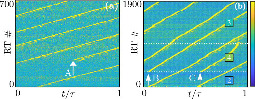
Figure 3: Pseudo-space representation of experimental time traces, with a feedback delay of 8.2ns, showing the effect of external perturbations (indicated by arrows) of different timings, for a 1-pulse (a) and a 2-pulse (b) regime.

In the experiment, the ability of an optical perturbation to trigger a second and a third sustained pulse trains has been shown in figure 1. Figure 3 highlights the influence of the perturbation timing on the long-term dynamics of the microlaser with delayed optical feedback. Panel (a) shows that a perturbation (labelled A) introduced far from a pre-existing pulse train can make the system switch to the 2-pulse regime, in excellent qualitative agreement with the theoretical results of figure 2(a). Had the perturbation been sent closer to an existing pulse, it would have either globally retimed the initial pulse train, leaving the system in the same state, if introduced slightly earlier; if introduced slightly later than the regenerated pulse, it would have had no effect since it would have fallen in the refractory period of the pre-existing pulse. The net effect in the two cases is the same, as far as the asymptotic state is concerned.

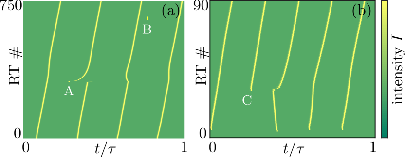
Figure 4: Pseudo-space representation of simulated time traces, showing the effect of external perturbations. In (a), starting from the stable 4-pulse regime, two perturbations are introduced before (A) and after (B) a reinjected pulse, leaving the system in the stable 4-pulse regime. In (b), the 5-pulse regime is approached from a transient regime with four pulses per round trip.

Figure 3(b) illustrates the influence of perturbations with different timings when two and three pulse trains pre-exist in the feedback cavity: starting from the 2-pulse regime, a third sustained pulse train is triggered by an optical perturbation (labelled B). The fourth perturbation (labelled C) is introduced shorty afterwards with a similar relative timing with respect to the two pre-existing pulses (i.e in the pseudo-space representation it appears to be half-way in between two pre-existing pulses). However, it only triggers a transient pulse; hence, it does not affect the long-term dynamics of the system which settles back on the 3-pulse solution after a few hundreds of round trips. As predicted by the theory in figure 2, these results confirm that triggering new sustained pulse trains becomes more and more challenging when the number of pre-existing pulse trains in the external cavity increases. In particular, figure 2(e) shows that an external perturbation cannot trigger a fifth sustained pulse train in the model when the system is in the 4-pulse regime. The temporal traces associated to this case are plotted in 4(a). As observed in the experiment, perturbations sent slightly before or after a pulse have no effect on the long term dynamics and leave the system in the same state. By contrast, figure 4(b) demonstrates that it is nevertheless possible to reach the 5-pulse solution by sending the fifth perturbation (labelled C) during the transient dynamics, when four pre-existing pulses are still far from their stable configuration. In general, all the stable $n$-pulse regimes can be accessed from suitable transient dynamics by addition of single or multiple perturbation pulses. Overall, the experiment and the numerical analysis show excellent qualitative agreement in terms of the influence of the perturbation timing on the long-term dynamics of the system.

We point out that, in the experiment, external perturbations can be sent either coherently (at the laser emission wavelength) or incoherently (at the pump wavelength) (Selmi et al., 2016), which corresponds in system (1) to perturbations on the intensity variable $I$ or on the gain variable $G$, respectively. The basins were also mapped with coherent perturbations $\Delta I$ on the intensity variable $I$. Apart from differences observed mainly in the finer details of the basin boundaries, which is related to intersections of higher dimension manifolds, the structure of the basins of attraction is qualitatively as those shown in figure 2(b)–(g). Interestingly, this strongly suggests that what does matter is the strength and timing of the perturbation, rather than the exact way the perturbation is introduced.

In conclusion, we have shown how any initial pulsing pattern equalizes to an equidistant pulse train in the excitable micropillar laser with delayed optical feedback. Different stable equalized periodic orbits with different number of pulses in the feedback loop are sustained, and they can be accessed by means of single optical input pulses. Our study of the basins of attraction has shown how that, depending on the timing, a new pulse can be added when the number of initial equalized pulses is low, or a pulse can be subtracted from a sequence when the number of initial equalized pulses is larger. The experimental and theoretical results are in good agreement and allow a clear interpretation of the observed physical phenomena, which are based on small pulse-to-pulse differences generated by the slow carrier dynamics of the gain and absorber media. They provide a global physical picture of the short-term and long-term dynamics of regenerative pulse coexistence.

In terms of memory applications, any input pulse pattern will necessarily converge to one of the sustained and stable equalized pulse trains. While the information encoded in non-equal pulse spacing will be lost in the medium to long term, this device has the ability to converge to a given number of pulses in the feedback loop from an imperfect input (Hertz et al., 2018). This approximation property is linked to the fine structure of the infinite-dimensional basins of attractions of the system, which we have mapped out here for the case of a single short optical perturbation.

Finally, we highlight that the result presented here are quite general in that they are generated only by excitability and delayed feedback. As such, we believe that they will be of relevance beyond the scope of laser dynamics for systems that encode information as pulse trains, e.g., those arising in neuroscience.

^∗These authors contributed equally to the work.

References

- Izhikevich (2007) E. Izhikevich, Dynamical Systems in Neuroscience: The Geometry of Excitability and Bursting. (The MIT press, 2007).
- Garbin et al. (2015) B. Garbin, J. Javaloyes, G. Tissoni, and S. Barland, Nat. Commun. 6, (2015).
- Marino and Giacomelli (2017) F. Marino and G. Giacomelli, Chaos 27, 114302 (2017).
- Kelleher et al. (2010) B. Kelleher, C. Bonatto, P. Skoda, S. P. Hegarty, and G. Huyet, Phys. Rev. E 81 (2010), 10.1103/physreve.81.036204.
- Romeira et al. (2016) B. Romeira, R. Avó, J. M. L. Figueiredo, S. Barland, and J. Javaloyes, Sci. Rep. 6 (2016).
- Terrien et al. (2017a) S. Terrien, B. Krauskopf, N. G. R. Broderick, L. Andréoli, F. Selmi, R. Braive, G. Beaudoin, I. Sagnes, and S. Barbay, Phys. Rev. A 96 (2017a), 10.1103/physreva.96.043863.
- Marconi et al. (2014) M. Marconi, J. Javaloyes, S. Balle, and M. Giudici, Phys. Rev. Lett. 112, 223901 (2014).
- Jang et al. (2015) J. K. Jang, M. Erkintalo, S. Coen, and S. G. Murdoch, Nat. Commun. 6, (2015).
- Camelin et al. (2016) P. Camelin, J. Javaloyes, M. Marconi, and M. Giudici, Phys. Rev. A 94, 063854 (2016).
- Javaloyes et al. (2016) J. Javaloyes, P. Camelin, M. Marconi, and M. Giudici, Phys. Rev. Lett. 116, 133901 (2016).
- Terrien et al. (2018) S. Terrien, B. Krauskopf, N. G. Broderick, R. Braive, G. Beaudoin, I. Sagnes, and S. Barbay, Opt. Lett. 43, 3013 (2018).
- Shastri et al. (2016) B. J. Shastri, M. A. Nahmias, A. N. Tait, A. W. Rodriguez, B. Wu, and P. R. Prucnal, Sci. Rep. 6, 19126 (2016).
- Foss et al. (1996) J. Foss, A. Longtin, B. Mensour, and J. Milton, Phys. Rev. Lett. 76, 708 (1996).
- Connors (2002) B. W. Connors, Nature 420, 133 (2002).
- Chaudhuri and Fiete (2016) R. Chaudhuri and I. Fiete, Nat. Neurosci. 19, 394 (2016).
- Ikeda et al. (1982) K. Ikeda, K. Kondo, and O. Akimoto, Phys. Rev. Lett. 49, 1467 (1982).
- Yanchuk and Perlikowski (2009) S. Yanchuk and P. Perlikowski, Phys. Rev. E 79, 046221 (2009).
- Nizette et al. (2006) M. Nizette, D. Rachinskii, A. Vladimirov, and M. Wolfrum, Physica D 218, 95 (2006).
- Selmi et al. (2016) F. Selmi, R. Braive, G. Beaudoin, I. Sagnes, R. Kuszelewicz, T. Erneux, and S. Barbay, Phys. Rev. E 94, 042219 (2016).
- Barbay et al. (2005) S. Barbay, Y. Ménesguen, I. Sagnes, and R. Kuszelewicz, Appl. Phys. Lett. 86, 151119 (2005).
- Elsass et al. (2010) T. Elsass, K. Gauthron, G. Beaudoin, I. Sagnes, R. Kuszelewicz, and S. Barbay, Eur. Phys. J. D 59, 91 (2010), 10.1140/epjd/e2010-00079-6.
- Barbay et al. (2011) S. Barbay, R. Kuszelewicz, and A. M. Yacomotti, Opt. Lett. 36, 4476 (2011).
- Selmi et al. (2014) F. Selmi, R. Braive, G. Beaudoin, I. Sagnes, R. Kuszelewicz, and S. Barbay, Phys. Rev. Lett. 112, 183902 (2014).
- Nahmias et al. (2013) M. A. Nahmias, B. J. Shastri, A. N. Tait, and P. R. Prucnal, IEEE J. Sel. Topics Quantum Electron. 19, 1 (2013).
- Prucnal et al. (2016) P. R. Prucnal, B. J. Shastri, T. F. de Lima, M. A. Nahmias, and A. N. Tait, Adv. Opt. Photonics 8, 228 (2016).
- Selmi et al. (2015) F. Selmi, R. Braive, G. Beaudoin, I. Sagnes, R. Kuszelewicz, and S. barbay, Opt. Lett. 40, 5690 (2015).
- Erneux and Barbay (2018) T. Erneux and S. Barbay, Phys. Rev. E 97 (2018), 10.1103/physreve.97.062214.
- Yamada (1993) M. Yamada, IEEE J. Quantum Electron. 29, 1330 (1993).
- Krauskopf and Walker (2012) B. Krauskopf and J. J. Walker, “Bifurcation study of a semiconductor laser with saturable absorber and delayed optical feedback,” in Nonlinear Laser Dynamics (Wiley-VCH Verlag GmbH & Co. KGaA, 2012) pp. 161–181.
- Giacomelli and Politi (1998) G. Giacomelli and A. Politi, Physica D 117, 26 (1998).
- Jang et al. (2013) J. K. Jang, M. Erkintalo, S. G. Murdoch, and S. Coen, Nat. Photonics 7, 657 (2013).
- Dubbeldam et al. (1999) J. L. A. Dubbeldam, B. Krauskopf, and D. Lenstra, Phys. Rev. E 60, 6580 (1999).
- Engelborghs et al. (2001) K. Engelborghs, T. Luzyanina, and G. Samaey, DDE-BIFTOOL v. 2.00: a Matlab package for bifurcation analysis of delay differential equations, Tech. Rep. (Department of Computer Science, KU Leuven, Leuven, Belgium, 2001).
- Sieber et al. (2015) J. Sieber, K. Engelborghs, T. Luzyanina, G. Samaey, and D. Roose, DDE-BIFTOOL v. 3.1 manual—bifurcation analysis of delay differential equations, Tech. Rep. (http://arxiv.org/abs/ 1406.7144, 2015).
- Terrien et al. (2017b) S. Terrien, B. Krauskopf, and N. G. R. Broderick, SIAM J. Appl. Dyn. Sys. 16, 771 (2017b).
- Pisarchik and Feudel (2014) A. N. Pisarchik and U. Feudel, Physics Reports 540, 167 (2014).
- Krauskopf et al. (2005) B. Krauskopf, H. M. Osinga, E. J. Doedel, M. E. Henderson, J. Guckenheimer, A. Vladimirsky, M. Dellnitz, and O. Junge, Int. J. Bifurcation Chaos 15, 763 (2005).
- Balachandran et al. (2009) B. Balachandran, T. Kalmár-Nagy, and D. E. Gilsinn, Delay differential equations (Springer, 2009).
- Krauskopf and Green (2003) B. Krauskopf and K. Green, J. Comput. Phys. 186, 230 (2003).
- Keane and Krauskopf (2018) A. Keane and B. Krauskopf, Nonlinearity 31, R165 (2018).
- Hertz et al. (2018) J. Hertz, A. Krogh, and R. G. Palmer, “Introduction to the theory of neural computation,” (CRC Press, 2018) Chap. 2, p. 11, The Associatve Memory Problem.