High-harmonic generation in solids

Abstract

We analytically and numerically investigate the emission of high-harmonic radiation from model solids by intense few-cycle mid-infrared laser pulses. In single-active-electron approximation, we expand the active electron’s wavefunction in a basis of adiabatic Houston states and describe the solid’s electronic band structure in terms of an adjustable Kronig-Penney model potential. For high-harmonic generation (HHG) from MgO crystals, we examine spectra from two-band and converged multiband numerical calculations. We discuss the characteristics of intra- and interband contributions to the HHG spectrum for computations including initial crystal momenta either from the $\Gamma-$point at the center of the first Brioullin zone (BZ) only or from the entire first BZ, demonstrating relevant contributions from the entire first BZ. From the numerically calculated spectra we derive cutoff harmonic orders as a function of the laser peak intensity that compare favorably with our analytical stationary-phase-approximation predictions and published data.

I Introduction

Exposed to intense laser fields gases and solids emit a spectrum of radiation that is strongly enhanced at and near frequencies corresponding to multiples of the driving laser frequency. Over the past two decades, this high-order harmonic generation (HHG) process has been carefully investigated in atomic gases, and the underlying generation mechanism - the emission of radiation by laser-electric-field-driven rescattered electrons - is well understood Le et al. (2009); Krausz and Ivanov (2009). While solids are being discussed theoretically for decades in view of their large electronic density possibly enabling the design of high-intensity sources of harmonic radiation Plaja and Roso-Franco (1992); Protopapas et al. (1997); Faisal and Kamiński (1996); Faisal and Kaminski (1997), HHG from solids has remained a matter of debate Ghimire et al. (2011); Wu et al. (2015); Vampa et al. (2014). Experimentally, it was first carefully scrutinized less than a decade ago by Ghimire et al.  Ghimire et al. (2011). Understanding the mechanisms of HHG in solids is an area of emerging research interest and part of the ongoing diversification of attosecond science from the study of atoms and molecules to more complex nanoparticles Li et al. (2016, 2017, 2018a) and solids Leone et al. (2014); Thumm et al. (2015); Ciappina et al. (2017); Kruchinin et al. (2018). This extension of attosecond science holds promise for promoting the development of novel table-top intense high-frequency radiation sources and our understanding of the light-induced electron dynamics in solids, a prerequisite for improved ultrafast electron-optical switches Luu and Wörner (2016); Ghimire and Reis (2019).

Compared to HHG in atomic gases, theoretical investigations of solid HHG have indicated striking new effects, such as multiple plateaus Ndabashimiye et al. (2016); Wu et al. (2015) in HHG spectra and a linear dependence of the HHG cutoff frequency on the peak electric-field strengths of the driving laser Wu et al. (2015); Vampa et al. (2015); Osika et al. (2017); Li et al. (2018b). These characteristics have been revealed by numerically solving either the time-dependent Schrödinger (TDSE) in single-active-electron (SAE) approximation Mücke (2011); Hawkins et al. (2015); Wu et al. (2015); Li et al. (2018b) or semiconductor Bloch equations (SBEs) Golde et al. (2008); Schubert et al. (2014); Meier et al. (1994); Vampa et al. (2014); Jiang et al. (2017, 2018); Li et al. (2018b). SAE-TDSE-based numerical models have employed basis-set expansions of the active electron’s wavefunction using either static Korbman et al. (2013) or adiabatic Krieger and Iafrate (1985); Wu et al. (2015) Bloch states.

SAE solutions of the TDSE can be expressed in terms of density matrices for convenient comparison with the SBE approach that introduces a phenomenological dephasing time to account for relaxation processes Haug and Koch (1998). An advantage of working within the SAE-TDSE framework is that the computational time for solving a system with $n$ electronic bands scales linearly with $n$, while it scales as ${n(n-1)/2}$ in SBE calculations Luu and Wörner (2016). For ${n>20}$ this leads to approximately one order of magnitude difference in computation time (cf., Ref. Wu et al. (2015), where 51 bands are included for solving the TDSE within a static Bloch basis). This is of relevance at high intensities of the driving laser, where calculations with a large number of bands are required to reveal the multiplateau structure of converged HHG spectra  Wu et al. (2015). SAE models have successfully explained the main features of HHG in atomic gases Le et al. (2009); Krausz and Ivanov (2009), which has motivated their transfer to describing HHG in solids Wu et al. (2015); Ndabashimiye et al. (2016).

In this work we develop a numerical model for solving the TDSE in SAE approximation employing a basis-set expansion of the electronic wavefunction in so-called “Houston states” that vary adiabatically with the instantaneous driving-laser electromagnetic field Wu et al. (2015); Lindefelt et al. (2004); Krieger and Iafrate (1985). The use of an adiabatic basis is advantageous for gaining physical insight into the underlying basic mechanisms for HHG in solids, since it allows the identification of two distinct processes, intra- and an interband emission, that operate in different spectral regions. In calculating HHG spectra from solids, we pay attention to the crystal momentum of the initial state and scrutinize contributions from different crystal momenta in the entire first Brillouin zone (BZ). In particular, we find that HHG spectra calculated by only including the initial crystal momentum at the center of the BZ (the $\Gamma-$point) Wu et al. (2015) noticeably differ from calculations that include initial crystal momenta in the entire BZ Vampa et al. (2014). It has been recently proposed that the range of crystal momenta used in SAE calculations should be used as an adjustable parameter for getting converged numerical HHG spectra Li et al. (2018b). In the present work we revisit this suggestion and analytically determine, based on a stationary-phase approximation, the range of initial crystal momenta needed for the computation of HHG spectra at a given accuracy.

We organized this paper as follows. In Sec. II we describe our theoretical framework. In particular, in Sec. II.1 we solve the TDSE by expanding the active electron’s wavefunction in an adiabatic basis (Sec. II.1.1), compare our approach with a density-matrix formulation of solid HHG (Sec. II.1.2), and show how the observables of interest in this work, intra- and interband yields, are retrieved from our numerical results (Sec. II.1.3). In Sec. II.2 we discuss solid HHG for a simplified two-band system distinuishing intra- (Sec. II.2.1) and interband (Sec. II.2.2) yields. In Sec. II.3 we analyze interband HHG within a stationary-phase approximation (Sec. II.3.1), which allows us to estimate the relevant range of crystal momenta $k$ (Sec. II.3.2) that need to be included when adding HHG contributions from different $k$ in the first BZ (Sec. II.3.3). In Sec. III we present and discuss our numerical results for HHG in a model MgO crystal. First, based on simplified two-band calculations, we analyze in Sec. III.1 $k$-resolved spectra for a specific field strength of the driving-laser pulse (Sec. III.1.1), field-strength-dependent spectra (Sec. III.1.2), and cut-off harmonic orders as a function of the field strengths (Sec. III.1.3). Next, in Sec. III.2, we analyze field-strength-dependent HHG spectra (Sec. III.2.1) and cutoff harmonic orders (Sec. III.2.2) for calculations that are converged in the number of included electronic bands. In several appendices, we add details of our theoretical analysis. We use atomic units (${q_{e}=m_{e}=\hbar=1}$) throughout this work, unless specified otherwise.

II Theory

II.1 Single-active-electron solution of the TDSE

We solve the TDSE,

$$\left[\frac{1}{2}\left(\hat{p}+A(t)\right)^{2}+V(x)\right]\left|\psi(t)\right>=i\frac{\partial}{\partial t}\left|\psi(t)\right>,$$ (1)

subject to the interaction of the active electron with both, a one-dimensional infinitely extended solid and an infrared (IR) external laser field ${E(t)}$. We represent the solid by a periodic potential ${V(x)=V(x+a)}$, with lattice constant $a$, and the laser field by a 10-cycle “flat-top” vector potential:

$$A(t) =-\int_{0}^{t}E\left(t^{\prime}\right)dt^{\prime}$$ (2)

$$=\frac{A_{0}}{2T}\sin(\omega_{0}t)\left\{\begin{tabular}[]{cl}$t$&\;, $0\leq t\leq 2T\;\,$\\ $2T$&\;, $2T\leq t\leq 8T\;\,$\\ $(10T-t)$&\;, $8T\leq t\leq 10T\;\,$\end{tabular}\right..$$

${\hat{p}=-i\frac{\partial}{\partial x}}$ denotes the momentum operator and $A_{0}$, $\omega_{0}$, and ${T=2\pi/\omega_{0}}$ the external vector-potential amplitude, frequency, and period, respectively. Since in our numerical simulation (Sec. III) the driving-laser wavelength is three orders of magnitude larger than $a$ and the classical excursion range of the active electron in the laser field, in solving Eq.(1) we can safely invoke the dipole approximation, ${A(x,\,t)\approx A(t)}$.

We model ${V(x)}$ as a Kronig-Penney potential Kronig et al. (1931); Atkins and Friedman (2005), which yields the dispersion relation

$$\cos(ak)=\cos(a\sqrt{2\varepsilon_{nk}})+\frac{V_{0}}{\sqrt{2\varepsilon_{nk}}}\sin(a\sqrt{2\varepsilon_{nk}})$$ (3)

for the valence (${n=v}$) and conduction bands (${n=c}$). The potential strength $V_{0}$ is adjusted to match the electronic band structure of the solid. While Eq. (3) needs to be solved numerically, the Kronig-Penney model potential provides a convenient basis set of 2-fold-degenerate orthonormal eigenstates and allows us to calculate transition matrix elements in a closed analytical form (see Sec. II.1.1 below and Appendix A).

II.1.1 Expansion in Houston states

Expanding solutions of Eq. (1),

$$\left|\psi_{k}(t)\right>=e^{-iA(t)x}\sum_{n}B_{nk}(t)e^{\left[-i\int_{0}^{t}\varepsilon_{n\kappa(t^{\prime})}dt^{\prime}\right]}\left|\phi_{n\kappa(t)}\right>,$$ (4)

in terms of Houston states ${\left|\phi_{n\kappa(t)}\right>}$, results in the set of coupled equations

$$i\dot{B}_{nk}(t) =-\sum_{n^{\prime}\neq n}B_{n^{\prime}k}(t)E(t)D^{nn^{\prime}}_{\kappa(t)}$$ (5)

$$\times\exp\left[i\int_{0}^{t}\Delta\varepsilon_{\kappa(t)}^{nn^{\prime}}dt^{\prime}\right]\,.$$

In Eq. (5) we define the energy difference between Houston states Krieger and Iafrate (1985); Wu et al. (2015) (also referred to as “band-gap energy”) ${\Delta\varepsilon_{\kappa(t)}^{nn^{\prime}}=\varepsilon_{n\kappa(t)}-\varepsilon_{n^{\prime}\kappa(t)}}$ and the transition dipole moments (TDMs)

$$D^{nn^{\prime}}_{\kappa(t)} =\frac{i\,P^{nn^{\prime}}_{\kappa(t)}}{\Delta\varepsilon_{\kappa(t)}^{nn^{\prime}}}\;\;\;(n\neq n^{\prime})$$ (6)

$$D^{nn}_{\kappa(t)} =0.$$

The TDMs are given in terms of the momentum-operator matrix elements Lindefelt et al. (2004)

$$P_{\kappa(t)}^{nn^{\prime}}=\frac{1}{a}\int_{0}^{a}\phi_{n{\kappa(t)}}^{*}(x)\frac{1}{i}\frac{\partial}{\partial x}\phi_{n^{\prime}{\kappa(t)}}(x)\,dx.$$ (7)

The diagonal elements,

$$P_{\kappa(t)}^{nn}=\frac{\partial\varepsilon_{n{\kappa(t)}}}{\partial{\kappa(t)}}\,,$$ (8)

are related to the band energy $\varepsilon_{n{\kappa(t)}}$ and correspond to the group velocity of an electron wave packet in band $n$. Since the elements ${P^{nn^{\prime}}_{\kappa(t)}}$ are real, the TDMs satisfy ${D^{nn^{\prime}}_{\kappa(t)}=-D^{n^{\prime}n}_{\kappa(t)}}$ and ${\left(D^{nn^{\prime}}_{\kappa(t)}\right)^{*}=D^{n^{\prime}n}_{\kappa(t)}}$ (Appendix A).

Houston states are adiabatic in the field-dressed time-dependent crystal momentum

$$\kappa(t)=k+A(t)\,,$$ (9)

and solve the Schrödinger equation

$$\left[\frac{\hat{p}^{2}}{2}+V(x)\right]\left|\phi_{n\kappa(t)}\right>=\varepsilon_{n\kappa(t)}\left|\phi_{n\kappa(t)}\right>.$$ (10)

They can be viewed as adiabatic Bloch states, with $\kappa(t)$ replacing the Bloch-state crystal momentum $k$. ${\kappa(t)}$ thus parameterizes the field-driven electronic evolution under the influence of the IR pulse out of an initial state with crystal momentum $k$ (Fig. 1). As for ordinary Bloch functions Ashcroft and Mermin (1976), Houston states with different initial (field-free) crystal momentum $k$ or different band indices $n$ are not coupled by the Hamiltonian in Eq. (10), yet evolve differently. Since Houston states for different initial momenta $k$ explore the electronic band $n$ distinctively, they will be referred to as “$k-$channels” in this work.

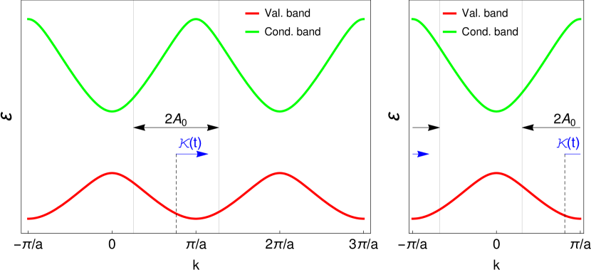
Figure 1: (Color online). The two lowest dispersion curves according Eq. (3) for the Kronig-Penney model in the repeated-zone scheme (left) and in the first BZ zone (right). The vertical black dashed line indicates a particular $k-$channel. The single-headed blue arrow shows the adiabatic momentum ${\kappa(t)}$ at time $t$, the double-headed arrow the maximum range (${2A_{0}}$) covered by ${\kappa(t)}$ within the first BZ.

II.1.2 Density-matrix formulation

The electronic evolution described in Eq. (5) can also be expressed in terms of the density operator,

$$\hat{\rho}(t)=\left|\psi_{k}(t)\right>\left<\psi_{k}(t)\right|\,,$$

in the pure state ${\left|\psi_{k}(t)\right>}$ given by Eq. (4). The matrix elements

$$\rho^{nn^{\prime}}_{k}(t) =B_{nk}(t)B_{n^{\prime}k}^{*}(t)$$

$$=\left<\phi_{n\kappa(t)}\right|\hat{\rho}_{k}\left|\phi_{n^{\prime}\kappa(t)}\right>e^{i\int_{0}^{t}\Delta\varepsilon_{\kappa(t^{\prime})}^{nn^{\prime}}}dt^{\prime}$$

represent band populations for ${n=n^{\prime}}$. Their time evolution is obtained by solving

$$i\dot{\rho}^{nn^{\prime}}_{k}(t) =E(t)\sum_{n^{\prime\prime}}[D^{n^{\prime\prime}n}_{\kappa(t)}e^{i\int_{0}^{t}\Delta\varepsilon_{\kappa(t^{\prime})}^{nn^{\prime\prime}}dt^{\prime}}\rho^{n^{\prime\prime}n^{\prime}}_{k}(t)$$

$$-D^{n^{\prime}n^{\prime\prime}}_{\kappa(t)}e^{i\int_{0}^{t}\Delta\varepsilon_{\kappa(t^{\prime})}^{n^{\prime\prime}n^{\prime}}dt^{\prime}}\rho^{nn^{\prime\prime}}_{k}(t)].$$ (11)

II.1.3 Intra- and interband yield

The electronic current in each ${k-}$channel,

$$J_{k}(t)=J_{k}^{ra}(t)+J_{k}^{er}(t),$$

consists of intra- and interband contributions,

$$J_{k}^{ra}(t) =-\sum_{n}\rho^{nn}_{k}(t)\,P^{nn}_{\kappa(t)}$$ (12)

and

$$J_{k}^{er}(t) =-\sum_{n^{\prime}>n}\sum_{n}e^{i\int_{0}^{t}\Delta\varepsilon_{\kappa(t^{\prime})}^{nn^{\prime}}dt^{\prime}}\,\rho^{n^{\prime}n}_{k}(t)P^{nn^{\prime}}_{\kappa(t)}+\text{c.c.},$$ (13)

respectively. It defines the spectral HHG yield from a given $k-$channel,

$$Y_{k}(\omega) =\left|\int_{-\infty}^{\infty}dt\,e^{-i\omega t}J_{k}(t)\right|^{2}\equiv\left|\hat{J}_{k}(\omega)\right|^{2}$$ (14)

$$=Y_{k}^{ra}(\omega)+Y_{k}^{er}(\omega)+2\hat{J}_{k}^{er}(\omega)\hat{J}_{k}^{ra}(\omega),$$

which, in addition to the intra- [$Y_{k}^{ra}(\omega)$] and interband [$Y_{k}^{er}(\omega)$] yields, includes the interference term $2\hat{J}_{k}^{er}(\omega)\hat{J}_{k}^{ra}(\omega)$.

For the dielectric solid analyzed in this work, the Fermi energy lies in the band gap between the highest occupied band (the valence-band) and the lowest unoccupied band (the first conduction band). Since the valence-band is fully occupied, we obtain the total HHG yield as

$$Y\left(\omega\right)=\left|\int_{-\infty}^{\infty}dt\,e^{-i\omega t}\int_{BZ}dk\,J_{k}(t)\right|^{2},$$ (15)

and corresponding expressions for the total intra- [${Y^{ra}(\omega)}$] and interband HHG yields [${Y^{er}(\omega)}$], after including current contributions from all ${k-}$channels, i.e. , from all crystal momenta $k$ in the first BZ.

II.2 HHG mechanism for a two-band system

In this subsection, we restrict the theory developed in Sec. II.1 to two electronic bands: the valence and first conduction band, even though more than two bands are required and included in our converged numerical calculations in Sec. III below. Designating the valence and conduction bands with superscripts $v$ and $c$, respectively, the intra- and interband currents in Eqs. (12) and (13) simplify to

$$J_{k}^{ra}(t) = -\rho^{vv}_{k}(t)\,P^{vv}_{\kappa(t)}-\rho^{cc}_{k}(t)\,P^{cc}_{\kappa(t)}$$ (16)

$$J_{k}^{er}(t) = -e^{-iS(k,\,t)}\rho^{cv}_{k}(t)P^{vc}_{\kappa(t)}+\text{c.c.}\,.$$ (17)

As detailed in Appendix C, Eq. (17) can be written as

$$J_{k}^{er}(t) = \frac{d}{dt}\left[\rho^{cv}_{k}(t)D^{vc}_{\kappa(t)}e^{-iS(k,\,t)}\right]-\Delta J_{k}^{er}(t)+\text{c.c.}$$ (18)

$$= \bar{J}^{er}_{k}(t)+\text{c.c.},$$

where we define

$$\Delta J_{k}^{er}(t) = \rho^{cv}_{k}(t)\dot{D}^{vc}_{\kappa(t)}e^{-iS(k,\,t)}\,,$$ (19)

$$\bar{J}^{er}_{k}(t) = \frac{d}{dt}\left[\rho^{cv}_{k}(t)D^{vc}_{\kappa(t)}e^{-iS(k,\,t)}\right]-\Delta J_{k}^{er}(t)\,,$$ (20)

and the action

$$S(k,\,t)=\int_{0}^{t}\Delta\varepsilon_{\kappa(t^{\prime})}^{cv}dt^{\prime}.$$

Applying Eq. (11) to the two-band system, we obtain

$$i\dot{\rho}^{cv}_{k}(t)=e^{iS(k,\,t)}\Delta\rho_{k}^{vc}(t)E(t)D^{vc}_{\kappa(t)},\,$$ (21)

with the population difference

$$\Delta\rho_{k}^{vc}(t)=\left[\rho^{vv}_{k}(t)-\rho^{cc}_{k}(t)\right],$$ (22)

and

$$i\dot{\rho}^{cc}_{k}(t)=E(t)D^{vc}_{\kappa(t)}e^{-iS(k,\,t)}\rho^{cv}(t)-\text{c.c.}\,.$$ (23)

Both, the SBE model for HHG in Refs. Vampa et al. (2014); Jiang et al. (2017); Li et al. (2018b) and the expansion of TSDE solutions in a Houston basis, use an adiabatic basis. Note that the SBE model in Refs. Vampa et al. (2014); Jiang et al. (2017); Li et al. (2018b) adds the damping term ${\rho^{cv}_{k}(t)/T_{2}}$ to Eq. (21), with an adjustable damping time $T_{2}$ for the interband coupling Haug and Koch (1998). In addition, it does not include the term ${\Delta J_{k}^{er}(t)}$ in Eq. (18). Therefore, the SBE model Vampa et al. (2014) and our SAE-TSDE cannot be expected to yield identical HHG spectra, not even for ${T_{2}\rightarrow\infty}$.

II.2.1 Intraband yield

For a two-band system, norm preservation demands ${\rho^{vv}_{k}(t)=1-\rho^{cc}_{k}(t)}$, such that the intraband current in Eq. (12) simplifies to

$$J_{k}^{ra}(t)=-P^{vv}_{\kappa(t)}+\rho^{cc}_{k}(t)\,\Delta P^{vc}_{\kappa(t)},$$ (24)

resulting in the interband yield

$$Y_{k}^{ra}(\omega)=\left|\int_{-\infty}^{\infty}dt\,e^{-i\omega t}\left[P^{vv}_{\kappa(t)}-\rho^{cc}_{k}(t)\,\Delta P^{vc}_{\kappa(t)}\right]\right|^{2},$$ (25)

where

$$\Delta P^{vc}_{\kappa(t)}=P^{vv}_{\kappa(t)}-P^{cc}_{\kappa(t)}.$$ (26)

At low laser intensities, the conduction-band population is very small (${\rho^{cc}_{k}(t)\ll 1}$), and, for every ${k-}$channel, the by far dominant contribution to the intraband HHG spectrum is generated by the term ${P^{vv}_{\kappa(t)}}$ in the intraband current. With increasing driving-field intensities, the second term (${\sim\rho^{cc}_{k}}$) gains significance.

Upon integration over the first BZ, the first term in Eq. (24) vanishes, due to symmetry, since ${P^{vv}_{k}}$ is an odd function of $k$ (Fig. 1). The integrated current is therefore given by

$$J^{ra}(t)=\int_{BZ}dk\,\rho^{cc}_{k}(t)\Delta P^{vc}_{\kappa(t)}\,,$$ (27)

leading to the intraband HHG yield for the two-band system

$$Y^{ra}(\omega)=\left|\int_{-\infty}^{\infty}dt\,e^{-i\omega t}\int_{BZ}dk\,\rho^{cc}_{k}(t)\Delta P^{vc}_{\kappa(t)}\right|^{2}\,.$$ (28)

At low intensities, even though each ${k-}$channel defines a significant intraband current, due to the symmetry-related cancellation of contributions from crystal momenta ${+k}$ and ${-k}$, the integrated intraband HHG yield is comparatively small.

II.2.2 Interband yield

Calculation of the HHG yield for a specific $k$-channel, according to Eq. (14), requires the Fourier-transformed current

$$\hat{\bar{J}}^{er}_{k}(\omega) =i\omega\int_{-\infty}^{\infty}dt\,e^{-i\omega t}\rho^{cv}_{k}(t)D^{vc}_{\kappa(t)}e^{-iS(k,\,t)}$$ (29)

$$-\int_{-\infty}^{\infty}dt\,e^{-i\omega t}\Delta J_{k}^{er}(t)\,.$$

Replacing ${\rho^{cv}_{k}(t)}$, obtained by integrating Eq. (21), in Eq. (18), the interband current and HHG yield for the two-band system become

$$\hat{\bar{J}}^{er}_{k}(\omega) =\omega\int_{-\infty}^{\infty}dt\,e^{-i\omega t}D^{vc}_{\kappa(t)}\,e^{-iS(k,\,t)}$$ (30)

$$\times\int_{0}^{t}dt^{\prime}\,e^{iS(k,\,t^{\prime})}\Delta\rho_{k}^{vc}(t^{\prime})E(t^{\prime})D^{vc}_{\kappa(t^{\prime})}$$

$$+\int_{-\infty}^{\infty}dt\,e^{-i\omega t}\Delta J_{k}^{er}(t)$$

and

$$Y_{k}^{er}(\omega)=\left|\hat{J}^{er}_{k}(\omega)\right|^{2}=\left|\hat{\bar{J}}^{er}_{k}(\omega)+\hat{\bar{J}}^{er}_{k}(-\omega)^{*}\right|^{2}\,,$$ (31)

respectively.

II.3 Approximate evaluation of the interband yield

While the numerical HHG spectra discussed in Sec. III below are calculated based on the theory outlined in Secs. II.1 and II.2, we apply in this subsection additional approximations to the interband current in order to derive analytical expressions that reveal additional physical properties of the interband HHG process in solids. We restrict this analysis to vector-potential amplitudes ${A_{0}<\pi/a}$, for which the range of ${\kappa(t)}$ is limited by the width, ${2\pi/a}$, of one BZ (Fig. 1).

II.3.1 Stationary-phase approximation

Setting the TDM in Eq. (30) equal to its value at the band center (${k=0}$) Vampa et al. (2014, 2015), ${D^{vc}_{\kappa(t)}\approx D^{vc}_{0}}$, remembering that according to Eq. (6) ${\left(D^{vc}_{0}\right)^{2}=-\left|D^{vc}_{0}\right|^{2}}$, and applying the frozen valence-band approximation Keldysh (1965) ${|\Delta\rho_{k}^{vc}(t)|\approx 1}$ Keldysh (1965), Eq. (30) simplifies to

$$\hat{\bar{J}}^{er}_{k}(\omega)\approx -\omega\left|D^{vc}_{0}\right|^{2}\int_{-\infty}^{\infty}dt\,\int_{0}^{t}dt^{\prime}\,e^{i\sigma_{\omega}(k,\,t,\,t^{\prime})}E(t^{\prime})\,,$$ (32)

where

$$\sigma_{\omega}(k,\,t,\,t^{\prime})=-\omega t-\int_{t^{\prime}}^{t}\Delta\varepsilon_{\kappa(t^{\prime\prime})}^{cv}dt^{\prime\prime}\,.$$ (33)

Since ${e^{i\sigma_{\omega}(k,\,t,\,t^{\prime})}}$ rapidly oscillates as a function of $t$ and ${t^{\prime}}$, the integrals in Eq. (32) are dominated by contributions at times ${t=t_{e}}$ and ${t^{\prime}=t_{s}}$ when the phase ${\sigma_{\omega}(k,\,t,\,t^{\prime})}$ is stationary, i.e.,

$$\frac{\partial\sigma_{\omega}(k,\,t_{e},\,t_{s})}{\partial t}=\frac{\partial\sigma_{\omega}(k,\,t_{e},\,t_{s})}{\partial t^{\prime}}=0\,.$$

At these times we find

$$\Delta\varepsilon_{\kappa(t_{e})}^{cv} =\omega$$ (34)

$$\Delta\varepsilon_{\kappa(t_{s})}^{cv} =0\,.$$ (35)

Evaluating Eq. (32) in stationary-phase approximation Lewenstein et al. (1994); Vampa et al. (2014); Wong (2001) now results in

$$\hat{\bar{J}}^{er}_{k}(\omega)\approx-\omega\left|D^{vc}_{0}\right|^{2}\sum_{t_{e}}\sum_{t_{s}}\frac{\left(2\pi i\right)E(t_{s})e^{i\sigma_{\omega}(k,\,t_{e},\,t_{s})}}{\left|\text{det}\left[\text{Hess }\sigma_{\omega}(k,\,t_{e},\,t_{s})\right]\right|^{1/2}}\,,$$ (36)

with the Hessian matrix

$$\left[\text{Hess }\sigma_{\omega}(k,\,t_{e},\,t_{s})\right]_{ij}=\left(\frac{\partial^{2}\sigma_{\omega}(k,\,t_{e},\,t_{s})}{\partial t_{i}\partial t_{j}}\right)_{t_{i},t_{j}=\,t_{e},\,t_{s}}\,.$$

Equation (34) implies that for each ${k-}$channel the cutoff frequency for interband HHG becomes

$$\omega^{c}(k,\,A_{0})=\left\{\begin{tabular}[]{lc}$\Delta\varepsilon_{|k|+A_{0}}^{cv}$&\;, $|k|+A_{0}<\pi/a\;\,$\\ $\Delta\varepsilon_{\pi/a}^{cv}$&\;, $|k|+A_{0}\geq\pi/a.\;$\end{tabular}\right.$$ (37)

Equation (35) cannot be fulfilled in our Kronig-Penney model for real-valued times and energies because the bandgap is nonzero across the entire BZ. We designate the maximal cutoff energy as ${\Delta\varepsilon_{max}^{cv}}$. Complying with Eq. (35) requests allowing for complex-valued times, energies, and crystal momenta $k$. Designating the complex crystal momentum as $K$, we analytically continue Eq. (35) and the transcendental Eq. (3) into the complex $K-$plane. Even though complex roots ${K_{s}=K(t_{s})}$ of Eq. (35) can only be obtained numerically, we get further insight into the interband HHG process by Taylor-expanding about ${K=0}$,

$$\Delta\varepsilon_{K}^{cv}=\Delta\varepsilon_{0}^{cv}+\frac{\text{d}\Delta\varepsilon_{0}^{cv}}{\text{d}K}K+\frac{1}{2}\frac{\text{d}\,^{2}\Delta\varepsilon_{0}^{cv}}{\text{d}K^{2}}K^{2}+\mathcal{O}(K^{3})\,.$$

While the expansion coefficients are in general complex, we show in Appendix B that ${\frac{\text{d}\Delta\varepsilon_{0}^{cv}}{\text{d}K}=0}$ and ${\Im\left[\frac{\text{d}^{2}\Delta\varepsilon_{0}^{cv}}{\text{d}K^{2}}\right]=0}$, such that

$$\Delta\varepsilon_{K}^{cv}=\Delta\varepsilon_{0}^{cv}+\frac{K^{2}}{2m^{*}_{0}}+\mathcal{O}(K^{3})\,,$$ (38)

where $\Im$ stands for “imaginary part of”. We evaluate the real-valued reduced effective mass,

$$m_{k}^{*}=\frac{m_{vk}^{*}m_{ck}^{*}}{m_{vk}^{*}-m_{ck}^{*}}\,,$$

at the band center,

$$m_{0}^{*}=\left.m_{k}^{*}\right|_{k=0}\,,$$

in terms of the valence- and conduction-band effective masses

$$\frac{1}{m_{nk}^{*}}=\frac{\partial^{2}\varepsilon_{nk}}{\partial k^{2}}\;,\;\;n=v,\,c\,.$$ (39)

Note that the derivatives in Eq. (39) are taken along the real axis and ${\varepsilon_{nk}=\Re[\varepsilon_{nK}]}$, where $\Re$ stands for “real part of”. Since the first term and the coefficient of the quadratic term in Eq. (38) are real, the roots $K_{s}$ are purely imaginary and correspond to interband transitions at the $\Gamma-$point (${k=0}$).

In Appendix D we show that, for a continuous-wave driving field of the form ${A_{0}\sin(\omega_{0}t)}$ and for ${\omega_{0}\sqrt{2\Delta\varepsilon_{0}^{cv}m_{0}^{*}}<E_{0}}$, the interband HHG yield is given by

$$Y^{er}_{k}(\omega) \approx\exp\left[-\frac{2\,\sqrt{2m^{*}_{0}}\,{\Delta\varepsilon_{0}^{cv}}^{3/2}}{E_{0}\sqrt{1-(k/A_{0})^{2}}}\right]$$ (40)

$$\times\left(2\pi\omega\right)^{2}\left|D^{vc}_{0}\right|^{4}E_{0}\sqrt{1-(k/A_{0})^{2}}\sqrt{\frac{m^{*}_{0}}{2\Delta\varepsilon_{0}^{cv}}}$$

$$\times\left|\sum_{t_{e}}\frac{e^{-i\omega t_{e}}\left[e^{i\left\{\Re[S(k,\,t_{s})]+S(k,\,t_{e})+\frac{\pi}{2}\right\}}+\text{c.c.}\right]}{\left|E(t_{e})\Delta P^{vc}_{\kappa(t_{e})}\right|^{1/2}}\right|^{2}\,.$$

Applying the effective mass theorem Ashcroft and Mermin (1976),

$$\frac{1}{m^{*}_{nk}}=1+2\sum_{n^{\prime}\neq n}\frac{(P_{k}^{nn^{\prime}})^{2}}{\Delta\varepsilon_{k}^{nn^{\prime}}}\,,$$

we obtain

$$m^{*}_{0}\approx\frac{1}{4\,\Delta\varepsilon_{0}^{cv}\left|D_{0}^{vc}\right|^{2}}\,.$$ (41)

This allows us to rewrite Eq. (40) as

$$Y^{er}_{k}(\omega) \approx\exp\left[-\frac{\sqrt{2}\,\Delta\varepsilon_{0}^{cv}}{E_{0}\left|D_{0}^{vc}\right|\sqrt{1-(k/A_{0})^{2}}}\right]$$ (42)

$$\times 2\left(\pi\omega\left|D^{vc}_{0}\right|\right)^{2}\left(\frac{E_{0}\left|D_{0}^{vc}\right|\sqrt{1-(k/A_{0})^{2}}}{\sqrt{2}\Delta\varepsilon_{0}^{cv}}\right)$$

$$\times\left|\sum_{t_{e}}\frac{e^{-i\omega t_{e}}\left[e^{i\left\{\Re[S(k,\,t_{s})]+S(k,\,t_{e})+\frac{\pi}{2}\right\}}+\text{c.c.}\right]}{\left|E(t_{e})\Delta P^{vc}_{\kappa(t_{e})}\right|^{1/2}}\right|^{2}.$$

As expected, the interband HHG yield increases with decreasing band gap ${\Delta\varepsilon_{0}^{cv}}$ and increasing TDM ${\left|D^{vc}_{0}\right|}$.

II.3.2 Relevant k-range for the interband HHG

The repeated-zone scheme in Fig. 1 shows that, for ${k>A_{0}}$ or ${k<-A_{0}}$, $0<|\kappa(t)|<2\pi/a$. Hence, $|\kappa(t)|$ does not reach the limits $0$ and $2\pi/a$, Eq. (35) cannot be satisfied, and contributions to HHG are restricted to the interval ${k\in(-A_{0},\,A_{0})}$ within the first BZ. For the symmetrical dispersion relation of the Kronig-Penney model (Fig. 1), the interband HHG yield in Eq. (42) is largest at the $\Gamma-$point.

With the upper limit for the integrated interband yield

$$Y^{er}(\omega)=\left|\int_{BZ}dk\,\hat{J}^{er}_{k}(\omega)\right|^{2}\leq\left(\int_{BZ}dk\,\left|\hat{J}^{er}_{k}(\omega)\right|\right)^{2}$$ (43)

and since ${\left[1-(k/A_{0})^{2}\right]^{1/2}\leq 1}$ in Eq. (42), we find the contribution of each $k$-channel to the interband yield to be limited by

$$\left|\hat{J}^{er}_{k}(\omega)\right| = \sqrt{Y^{er}_{k}(\omega)}$$ (44)

$$\propto \,\exp{\left[-\frac{\Delta\varepsilon_{0}^{cv}}{\sqrt{2}E_{0}\left|D_{0}^{vc}\right|\sqrt{1-(k/A_{0})^{2}}}\right]}\,.$$

We can now estimate the range ${k_{max}(A_{0})}$ of initial-state crystal momenta ${k\in\left(-\frac{k_{max}(A_{0})}{2},\frac{k_{max}(A_{0})}{2}\right)}$ that yield relative contributions larger than ${10^{-N}}$ times the maximal yield $Y^{er}_{0}(\omega)$,

$$Y^{er}_{k}(\omega)\geq 10^{-N}Y^{er}_{0}(\omega),$$

as

$$k_{max}(A_{0}) \approx\frac{2E_{0}}{\omega_{0}}$$ (45)

$$\times\sqrt{1-\left[\frac{\Delta\varepsilon_{0}^{cv}}{\sqrt{2}E_{0}\left|D_{0}^{vc}\right|\left(\frac{N}{2}\ln 10+\frac{\sqrt{2}\,\Delta\varepsilon_{0}^{cv}}{E_{0}\left|D_{0}^{vc}\right|}\right)}\right]^{2}}\,.$$

II.3.3 Integrated interband yield

In this subsection we examine the net contribution to the interband current from all $k$-channels in the first BZ to obtain the observable integrated interband yield ${Y^{er}(\omega)}$. For numerical applications, the numerical effort can possibly be reduced by limiting the integration range to ${k_{max}(A_{0})}$, as determined in the previous subsection. Whether this is possible depends on the specific laser parameters and solid electronic structure.

Equation (29) leads to the interband current, integrated over the whole BZ,

$$\hat{\bar{J}}^{er}(t) =\int_{BZ}dk\left[\omega\int_{-\infty}^{\infty}dt\,e^{-i\omega t}\rho^{cv}_{k}(t)D^{vc}_{\kappa(t)}e^{-iS(k,\,t)}\right.$$ (46)

$$\left.-\int_{-\infty}^{\infty}dt\,e^{-i\omega t}\Delta J_{k}^{er}(t)\right]\,.$$

For constant TDMs and a frozen valence-band population, we arrive at the saddle-point conditions

$$\frac{\partial\sigma_{\omega}(k_{r},\,t_{s},\,t_{e})}{\partial k}=\frac{\partial\sigma_{\omega}(k_{r},\,t_{s},\,t_{e})}{\partial t}=\frac{\partial\sigma_{\omega}(k_{r},\,t_{s},\,t_{e})}{\partial t^{\prime}}=0\,,$$

with ${\sigma_{\omega}(k,\,t^{\prime},\,t)}$ defined in Eq. (33). These conditions imply

$$\Delta\varepsilon_{\kappa_{r}(t_{s})}^{cv} = 0$$ (47)

$$\int_{t_{s}}^{t_{e}}\Delta P^{vc}_{\kappa_{r}(t)}dt = 0$$ (48)

$$\Delta\varepsilon_{\kappa_{r}(t_{e})}^{cv} = \omega,$$ (49)

where ${\kappa_{r}(t)=k_{r}+A(t)}$, and allow us to determine the roots $k_{r}$, $t_{s}$, and $t_{e}$ numerically.

Equations (47) and (49) are equivalent to Eqs. (35) and (34). Condition (48) arises due to the integration over the BZ. It expresses the requirement of the excited photoelectron wave packet, moving with group velocity ${P^{cc}_{k_{r}+A(t)}}$, and the residual hole wave packet, propagating with group velocity $P^{vv}_{k_{r}+A(t)}$, to recombine at time $t_{e}$ after their birth at time $t_{s}$, while emitting a photon with energy ${\Delta\varepsilon_{\kappa_{r}(t_{e})}^{cv}}$. We show in Appendix E that, since ${\Im[t_{s}]\propto\omega_{0}\sqrt{2\Delta\varepsilon^{cv}_{0}m_{0}^{*}}}$ and the matrix elements $P^{nn}_{k}$ are odd functions of $k$, Eq. (48) can be approximated as

$$\int_{t_{0}}^{t_{e}}\Delta P^{vc}_{\kappa_{r}(t)}dt\approx 0\,.$$ (50)

Even though within the Kronig-Penney model the band-gap energy ${\Delta\varepsilon_{k}^{cv}}$ grows continuously from the center to the edge of the first BZ, the $k-$channel at ${k=k_{r}^{c}}$ with the largest frequency,

$$\omega^{c}_{BZ}(A_{0})=\varepsilon_{k_{r}^{c}+A(t_{e})}\,,$$ (51)

lies in the range ${k_{r}\in(-A_{0},\,A_{0})}$, as seen in Sec. II.3.2, and needs to be determined numerically (see Sec. III.2.1 for a specific numerical example).

In analogy to Eq. (36), we obtain the Fourier-transformed net interband current as

$$\hat{\bar{J}}^{er}(\omega) \approx-\omega\left|D^{vc}_{0}\right|^{2}\,\left(2\pi i\right)^{3/2}$$ (52)

$$\times\sum_{|k_{r}|<A_{0}}\sum_{t_{e}}\sum_{t_{s}}\frac{E(t_{s})e^{i\sigma_{\omega}(k_{r},\,t_{e},\,t_{s})}}{\left|\text{det}\left[\text{Hess }\sigma_{\omega}(k_{r},\,t_{e},\,t_{s})\right]\right|^{1/2}}\,.$$

This expression is equivalent to

$$\hat{\bar{J}}^{er}(\omega) \approx-\omega\left|D^{vc}_{0}\right|^{2}\,\left(2\pi i\right)^{3/2}$$ (53)

$$\times\sum_{|k_{r}|<A_{0}}\sum_{t_{e}}\sum_{t_{s}}E(t_{s})e^{i\sigma_{\omega}(k_{r},\,t_{e},\,t_{s})}$$

$$\times y^{cv}_{\kappa_{r}}(t_{e},t_{s})\,,$$

where

$$y^{cv}_{\kappa_{r}}(t_{e},t_{s}) =\left|\sqrt{\frac{2\Delta\varepsilon_{0}^{cv}}{m_{0}^{*}}}E(t_{e})\Delta P^{vc}_{\kappa_{r}(t_{e})}\right|^{-1/2}$$ (54)

$$\times\left|\left[\sqrt{\frac{2\Delta\varepsilon_{0}^{cv}}{m_{0}^{*}}}+iE(t_{s})\int_{t_{s}}^{t_{e}}dt\frac{1}{m^{*}_{\kappa_{r}(t)}}\right]\right|^{-1/2}\,,$$

resulting in the approximated integrated interband yield

$$Y^{er}(\omega) \approx(2\pi)^{3}\left(\omega\left|D^{vc}_{0}\right|\right)^{2}$$ (55)

$$\times|\sum_{|k_{r}|<A_{0}}E(t_{s})\,e^{\left[-\frac{\sqrt{2}\,\Delta\varepsilon_{0}^{cv}}{E_{0}\left|D_{0}^{vc}\right|\sqrt{1-(k_{r}/A_{0})^{2}}}\right]}\,$$

$$\times\sum_{t_{e}}\left[e^{-i\omega t_{e}}e^{i\left\{\Re[S(k,\,t_{s})]+S(k,\,t_{e})+\frac{3\pi}{2}\right\}}+\text{c.c.}\right]$$

$$\times y^{cv}_{\kappa_{r}}(t_{e},t_{s})|^{2}\,.$$

III Numerical Results

For our numerical applications of the theoretical model described in Sec. II, we adopt the laser wavelength (3250 nm) and pulse duration (10 optical cycles) of the experiment by Ghimire et al.  Ghimire et al. (2011) and the temporal pulse profile given by Eq. (2). We model the electronic structure of MgO based on the Kronig-Penney model potential [Eq. (56)] with an interlayer spacing of ${a=8}$ a.u. Xu and Ching (1991) and adjust the potential strength to ${V_{0}=22.345}$ eV in order to reproduce the bandgap energy between the valence and conduction band at the $\Gamma-$point, 4.19 eV, obtained by Xu and Ching Xu and Ching (1991) from a full-dimensionality orthogonalized-linear-combination-of-atomic-orbitals (OLCAO) calculation within the framework of density-functional theory (DFT) in local density approximation (LDA). These values of the Kronig-Penney potential parameters result in a local bandgap at the BZ edge (at ${k=\pm\pi/a}$) of 13.6 eV, in very good agreement with the local bandgap at the $X$ point of 13 eV computed by Xu and Ching (Fig. 2).

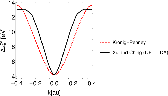
Figure 2: (Color online). Bandgap energies in the first BZ between the valence and lowest conduction band of MgO obtained within the Kronig-Penny model with interlayer spacing of 8 a.u. and potential strength 22.345 eV (black solid line) and adapted from the OLCAO-LDA DFT calculation of Ref. Xu and Ching (1991) along the $\Gamma-X$ direction (dashed red line).

In this section, we perform a systematic numerical study of the contributions to the HHG spectrum from different $k$ channels within the entire first BZ. We first discuss results obtained by restricting the external-field-driven electron dynamics to the valence and conduction band in Sec. III.1, before presenting converged HHG spectra obtained by including up to 13 electronic bands of MgO in Sec. III.2. For all calculations we employed a fourth-order Runge-Kutta algorithm to numerically solve Eq. (5) at 400 equally spaced ${k-}$points in the first BZ.

III.1 HHG spectra in two-band approximation

In order to understand the basic mechanisms of intra- and interband HHG in solids, we complement our theoretical analysis of HHG by a two-band system in Sec. II.2 above, with the numerical solution of Eq. (5), restricted to the lowest (highest) conduction (valence) band of MgO. While this approach can only provide acceptable results at moderate intensities of the driving field (${A_{0}<\pi/a}$), it fails at higher field strengths, for which the inclusion of more bands is mandatory (Sec. III.2).

III.1.1 Lattice-momentum-resolved contributions to HHG

To reveal the characteristics of HHG spectra, including all $k$-channels in the first BZ, we performed a calculation at a field strength of ${0.13\,\text{V/\AA}}$. Figures 3 (a) - 3 (c) display two-band HHG spectra as a function of the lattice momentum $k$. While, according to Eq. (14), the total yield is not equal to the sum of the intra- and interband yield, it is instructive to examine intra- and interband spectra separately. The comparison of Figs. 3(a) and 3(b) shows that intraband harmonics dominate HHG at harmonic photon energies below the band gap, ${\Delta\varepsilon_{0}^{cv}\approx 11\omega_{0}}$, while above this threshold mainly interband harmonics contribute to the total HHG yield in Fig. 3(c). The observation that the band gap establishes a threshold between intra- and interband HHG is consistent with energy conservation, requiring electronic probability density to cross the local band gap, ${\Delta\varepsilon_{\kappa(t)}^{cv}}$, before contributing to the interband current and thus to the interband HHG.

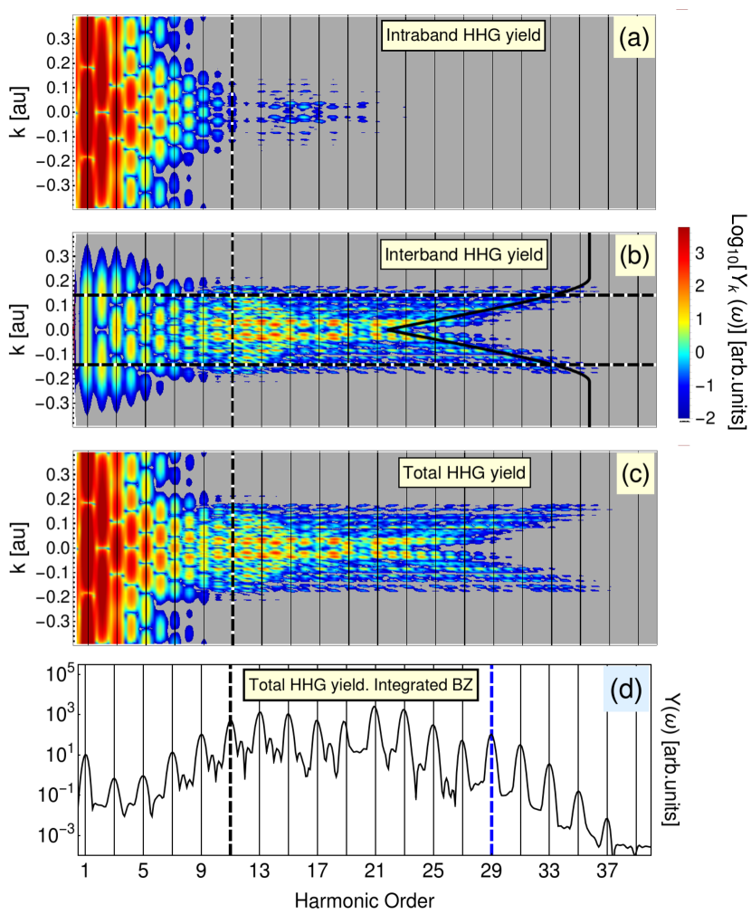
Figure 3: (Color online). HHG in MgO driven by a 10-cycle 3250 nm pulse with a peak electric-field strength of ${0.13\,\text{V/\AA}}$ (corresponding to a peak intensity of $2.24\times 10^{11}$ W/cm²). Thin vertical lines mark odd harmonics. The vertical black dashed line indicates the harmonic order ($\Delta\varepsilon_{0}^{cv}/\omega_{0}=11$) corresponding to the minimum band-gap energy $\Delta\varepsilon_{0}^{cv}$ at $k=0$. (a) Intraband HHG spectrum. (b) Interband HHG spectrum. The horizontal dashed black lines indicate ${\pm k_{max}(A_{0})/2}$ for $N=5$ as given by Eq. (45). The V-shaped black line shows the maximal band-gap energy $\omega^{c}(k,\,A_{0})$ as given by Eq. (37). (c) Total HHG spectrum. The yields in (a-c) are given as functions of the lattice momentum $k$ over the entire first BZ and on the same logarithmic scale. (d) Total HHG yield, integrated over the first BZ. Above harmonic order 29, the yield drops exponentially, determining the cutoff energy indicated by the vertical blue dashed line.

In view of Eq. (24) and the semiclassical interpretation of $P^{vv}_{\kappa(t)}$ as the photoelectron group velocity in the valence band, at low electric-field strengths we expect the intraband yield [Eq. (25)] to be dominated by the Fourier transform of $P^{vv}_{\kappa(t)}$ (Fig. 4). Indeed, below the interband-gap threshold (11th harmonic), the yields in Figs. 3(a) and 4 very closely resemble each other and are identical with respect to their zeros along the $k$-axis for every given harmonic order: both spectra exhibit even and odd harmonics that vary over the first BZ. At the $\Gamma-$point and edge of the first BZ both spectra only include odd harmonics.

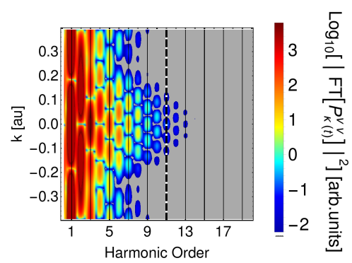
Figure 4: (Color online). Time Fourier transformation of the valence-band group velocity ${P^{vv}_{\kappa(t)}}$ for a 10-cycle 3250 nm laser pulse of ${0.13\,\text{V/\AA}}$ peak field strength.

Below the interband-gap threshold, the interband spectrum in Fig. 3(b) bears some similarity with the intraband yield in Fig. 3(a), but has significantly lower yields and a different distribution of yield nodes along the $k$-axis, at all harmonic orders. Above the interband-gap threshold, the interband yield has a rich $k$-dependent structure of even and odd harmonics. According to Eq. (37), the spectral range of interband high-order harmonics above the interband-gap threshold at the 11th harmonic is limited by ${\omega^{c}(k,\,A_{0})}$ . This $k$-dependent upper limit is indicated in Fig. 3(b) by the V-shaped solid black line. According to Eq. (45), contributions to the interband yield from $k$-channels that are $N$ orders of magnitude smaller than the maximal yield at the $Gamma$-point lie in the range ${\pm k_{max}(A_{0})/2}$. The V-shaped solid black line shows their onset for ${N=5}$.

We note that our numerical yields in Fig. 3, including contributions to HHG for $k$-channels within the entire first BZ, are incompatible with the assumption in previous studies Ghimire et al. (2012); Wu et al. (2015) that only a small part of the first BZ near the ${\Gamma-}$point contributes to HHG in solids. Even though for the one-dimensional model solid investigated here computing time is not an issue, the limit imposed by Eq. (45), and its numerical validation in Fig. 3, in addition to providing physical insight into the HHG process, is relevant for reducing the computational effort in multi-band HHG calculations based on a three-dimensional representation of the solid.

While the $k$-channel-resolved HHG spectrum in Fig. 3(c) includes even and odd high-order harmonics and depends in a rather complex way on the harmonic photon energy and lattice momentum $k$, including contributions to HHG from the entire first BZ according to Eq. (15), results in the comparatively simple total HHG spectrum shown in Fig. 3(d). As expected due to the inversion symmetry about the $\Gamma-$point of the Kronig-Penney band structure (Fig. 1), the total HHG spectrum in Fig. 3(d) is strongly dominated by odd harmonics.

III.1.2 Field-strength dependence of HHG spectra

Figure 5 shows the total HHG yield (including intra- and interband HHG) for the ${k=0}$ channel, i.e., only including the ${\Gamma-}$point at the center of the first BZ, for peak electric-field strengths ${0.05\,\text{V/\AA}<E_{0}<0.3\,\text{V/\AA}}$. This field-strength range corresponds to the laser-peak-intensity range ${3.3\times 10^{10}\,\text{W/cm}^{2}<\,I_{0}\,<1.19\times 10^{12}\,\text{W/cm}^{2}}$. We chose the upper limit of this interval to slightly exceed the field strength ${(\pi/a)\omega_{0}^{-1}\approx 0.283\,\text{V/\AA}}$. At this field strength, the vector-potential amplitude is ${A_{0}=\pi/a}$, such that the field-dressed time-dependent crystal momentum ${\kappa(t)=k+A(t)=A(t)}$ defined in Eq. (9) explores the entire first BZ (Fig. 1) within one optical cycle in the plateau of the laser pulse and, thus, the entire range of local band gaps. We selected the lower limit of the field strength in view of the approximations made in Sec. II.2, which are based on a series expansion in the parameter ${\gamma=\omega_{0}\sqrt{2\Delta\varepsilon_{0}^{cv}m^{*}_{0}}/E_{0}}$. Requesting ${\gamma<1}$, implies for MgO ${E_{0}>0.1\,\text{V/\AA}}$, slightly above the lower limit of the assumed range of field strengths.

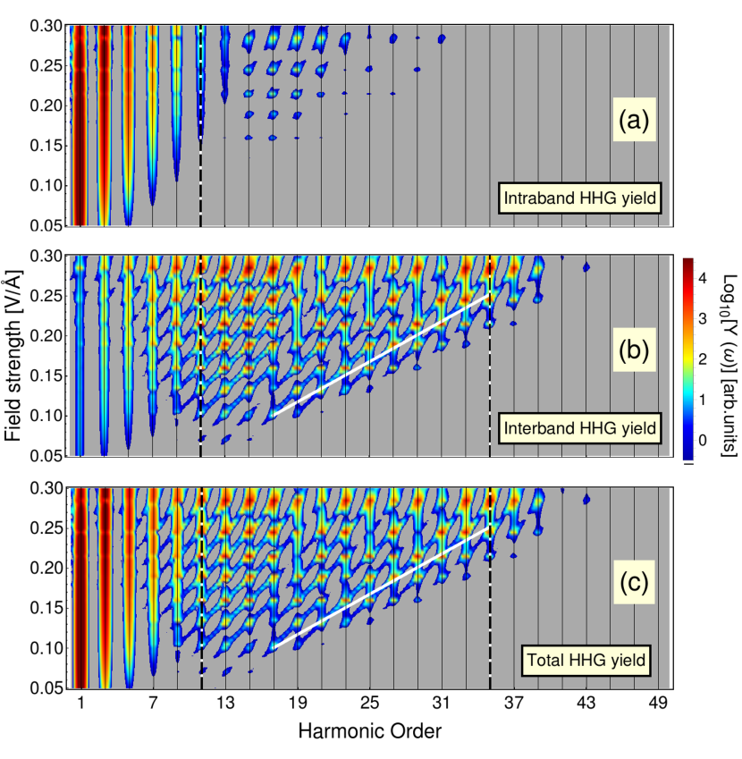
Figure 5: (Color online). HHG in MgO driven by a 10-cycle 3250 nm pulse as a function of peak laser-electric-field strength. Contributions to the HHG yield from the ${k=0}$ channel ($\Gamma-$point) only. (a) Intraband, (b) interband, and (c) total spectra. Thin vertical lines mark odd harmonics. The vertical black dashed lines correspond to the minimal and maximal local band-gap energies ${\Delta\varepsilon_{0}^{cv}}$ and ${\Delta\varepsilon_{max}^{cv}}$ in the first BZ. The white line in (b,c) indicates the cutoff harmonic order.

The comparison of the intra- and interband yields in Figs. 5(a) and  5(b) shows that the intraband emission dominates the total yield in Fig. 5(c) below and interband emission above the band-gap threshold near the 11th harmonic, for the entire considered range of electric-field strengths. The HHG cutoff is thus determined by interband emission and displayed as superimposed white lines in Figs. 5(b) and  5(c). We analyze the HHG cutoff behavior in more detail in Sec. III.1.3 below. Over the range of displayed electric-field strengths the intra- and interband spectra are dominated by odd harmonics, with slim traces of even harmonics. Small even and non-integer HHG yields were also noticed in an SBE-based calculation by Li et al.  Li et al. (2018b) and explained in terms of the combined effect of the external-field and time dependence of the TDM $D^{vc}_{\kappa(t)}$. We speculate that this effect may be enhanced due to our inclusion of the term defined by Eq. (19) in Eq. (18). This term is absent in the SBE model.

Relaxing the ${k=0}$-channel ($\Gamma$-point) emission restriction, Fig. 6 shows yields obtained after integrating $k$ over the first BZ. As for the $\Gamma$-point-only yield in Fig. 5, the comparison of the intra-, interband, and total yields in Figs. 6(a), 6(b), and 6(c), respectively, reveals for the entire shown laser-peak-intensity range that below the lowest band-gap threshold, near the 11th harmonic, the yields are dominated by intraband emission, while above this threshold practically only interband emission occurs. Even though the spectra include traces of even and non-integer harmonics (as they do for $\Gamma-$point-only emission), the contrast between odd and even harmonic yields is larger than for $\Gamma$-point-only emission.

As discussed in the preceding Sec. III.1.1, intraband emission at the $\Gamma-$point is directly related to the valence-band group velocity. It yields intense odd and even harmonics, as seen in Figs. 3 and 4. On the other hand, as given by Eq. (27), upon integration over the first BZ the valence-band term in Eq. (25) cancels (by symmetry), and high-yield emission requires the laser-electric field to be strong enough to effectively promote electrons to the conduction band. This explains the low yield at low intensities in Figs. 6(b) and 6(c), as compared to the corresponding $\Gamma-$point-only yields in Fig. 5. The experimental investigation of HHG below the lowest band-gap threshold and for low to moderate peak intensities might thus resolve the range ${k_{max}(A_{0})}$ of carriers involved in HHG for a specific substrate. However, it remains to be explored to what extent experimental focal-volume effects, i.e., averaging of the laser intensity profile, prevent the accurate determination of ${k_{max}(A_{0})}$.

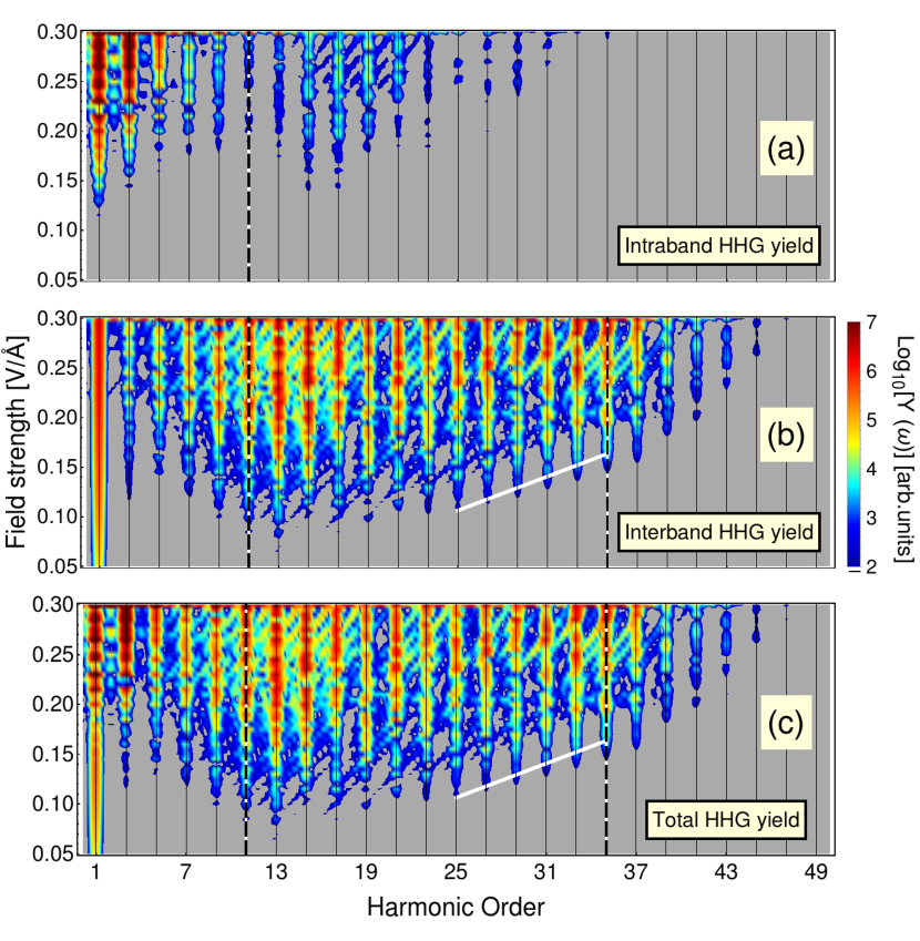
Figure 6: (Color online). As Fig. 5, but integrated over initial $k$-channels from the entire first BZ.

III.1.3 Field-strength dependence of the HHG cutoff

In this subsection we analyze the field-strength dependence of the HHG cutoff frequency obtained including both, $\Gamma-$point-only emission and $k$-channels from the entire first BZ. As the comparison of interband and total yields in Figs. 5 and 6 reveals, inclusion of the entire first BZ increases the highest generated frequencies, as compared to $\Gamma-$point-only emission. For each given peak electric-field strength, we visually determine the cutoff as the HHG order at which the yield starts to decline exponentially (as indicated in Fig. 3(d)), for both $\Gamma-$point-only and BZ-integrated yields. This leads to the intensity-dependent cutoff shown by the markers in Fig. 7. For the shown range of harmonic orders, inclusion of all $k$-channels results in cutoffs (indicated as triangular markers) in good agreement with our saddle-point prediction (green dotted line) that lie 8 - 10 harmonic orders above the cutoff for $\Gamma-$point-only emission (square markers). The cutoff orders predicted for the $\Gamma$-point-only emission by our 2-band TDSE calculations and our saddle-point analysis (red dashed line) are in fair agreement with the 2-band TDSE results of Wu et al.  Wu et al. (2015) (solid blue blue line), which we adapted from Fig. 3(b) in Ref. Wu et al. (2015). In agreement with Wu et al. , we find that the cutoff increases approximately linearly with laser peak-electric-field strength over the displayed range of harmonic orders, albeit with a noticeably smaller slope.

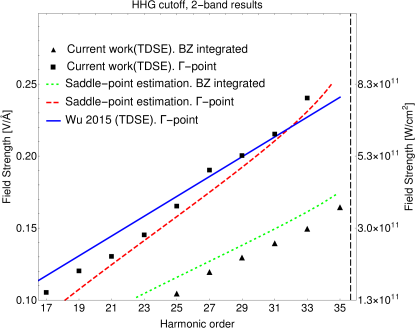
Figure 7: (Color online). Dependence of HHG-cutoff order on the laser peak-electric-field strength (left vertical axis) or intensity (right vertical axis) in two-band approximation. Square markers show HHG cutoffs for $\Gamma-$point-only (${k=0}$) emission. Triangular markers indicate HHG cutoffs including $k$-channels from the entire first BZ. The red dashed and green solid line show approximate cutoffs obtained from the saddle-point equations in Secs. II.3.1 and II.3.3 for $\Gamma-$point-only emission and $k$-channels from the entire first BZ, respectively. The dashed red line, in particular, is given by Eq. (37). The solid blue line shows 2-band TDSE results adapted from Fig. 3(b) in Wu et al.  Wu et al. (2015) for $\Gamma-$point-only emission.

To better understand the field-strength dependence of the HHG cutoff, we resort to the saddle-point analysis of the HHG process in the 2-band approximation discussed in Secs. II.3.1 and II.3.3. Referring to HHG including all $k$-channels in the first BZ, we numerically solve the saddle-point Eq. (50) for $t_{e}$ and subsequently Eq. (49) for each $k_{r}$. This yields the frequency curve $\Delta\varepsilon_{\kappa_{r}(t_{e})}^{cv}$, from which we get the maximal frequency $\omega^{c}_{BZ}$ and cutoff harmonic order $\omega^{c}_{BZ}/\omega_{0}$. The red line in Fig. 8, shows the harmonic energy ${\Delta\varepsilon_{\kappa_{r}(t_{e})}^{cv}}$ as a function of values for $k_{r}$ that contribute to the BZ-integrated interband yield for a peak field strength of the driving laser of ${0.13\text{V/\AA}}$. As discussed in Sec. II.3.3, ${|k_{r}|<A_{0}}$ (indicated by vertical thin blue lines). The maximum harmonic energy is obtained at crystal momenta ${\pm k_{r}^{c}}$ indicated by the dotted green lines. $k$-channels with ${k=\pm k_{r}^{c}}$ thus yield the maximum cutoff energy at the given laser field strength. The V-shaped black solid line in Fig. 8 shows the maximum energy ${\omega^{c}(k,A_{0})}$, i.e., the electron-hole-pair-recombination energy in each $k-$channel given by Eq. (37) [cf., Fig. 3(b)]. This energy depends on the maximum local band gap in each channel and exceeds the cutoff energy in the BZ-integrated yield $\Delta\varepsilon_{\kappa_{r}(t_{e})}^{cv}$ (red line). Since $\omega^{c}(k_{r},A_{0})\approx\Delta\varepsilon_{\kappa_{r}(t_{e})}^{cv}$ the ${k=\pm k_{r}^{c}}$ channels have the largest contribution the HHG yield.

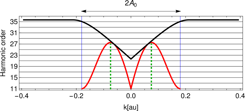
Figure 8: (Color online). Determination of the cutoff HHG order for a driving-laser peak intensity of ${0.13\text{V/\AA}}$ and a model MgO crystal with interlayer spacing $a=8$ a.u.. The black solid line shows the maximum local vertical band-gap energy at the field-dressed crystal momentum ${\kappa(t)=k+A(t)}$ during one optical cycle of the driving laser as a function of the field-free crystal momentum ${k\in[-\pi/a=-0.39,\pi/a=0.39]}$ a.u.. The vertical thin blue lines indicate crystal momenta ${\pm k_{r}}$, determined in stationary-phase approximation, that maximize the interband HHG yield ${Y^{er}(\omega)}$ given in Eq. (55). The red line shows the interband HHG cutoff in each $k$ channel. The vertical green dotted lines indicate the highest cutoff energies reached at crystal momenta $k_{r}^{c}$ that do not need to coincide with the maximum vertical band gap at the first BZ edge (${k=\pi/a}$).

III.2 Multiband spectra

III.2.1 Field-strength dependence of HHG spectra

Figures 9 and 10 show multiband HHG spectra for both the $\Gamma$-point-only and BZ-integrated calculations, respectively. Including the lowest 13 bands of the Kronig-Penney model MgO crystal, we find these spectra to have converged. The convergence of the results was determined from the evaluation, in the $k=0$ channel, of the population $\rho^{MM}_{0}(t)$ in each new band $M$ we added to the calculation. Based on our convergence criterium $\rho^{MM}_{0}(t)<10^{-12}\rho^{vv}_{0}(0)$, we find $M=13$ for a maximum peak field strength of ${E_{0}=0.3\,\text{V/\AA}}$. We included the same number (13) of bands for calculations at lower field strengths and for $k\neq 0$. Comparison with the two-band yields of Figs. 5 and 6 shows that the spectral region below the first band-gap threshold is dominated by the electron dynamics in the lowest two bands. For harmonic orders below $\approx 35$, the shape of the multiband spectra and their laser-electric-field dependence largely resemble the two-band spectra. Our numerical tests showed that the inclusion of more than two bands gradually improves the agreement with fully converged spectra in the shown spectral range.

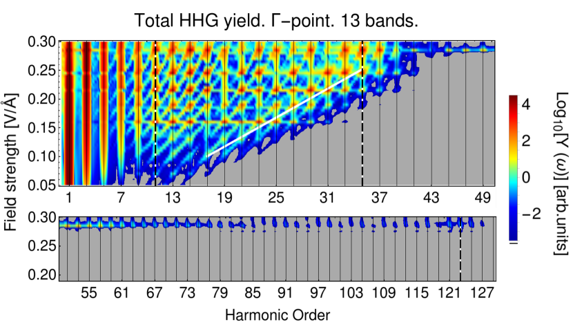
Figure 9: (Color online). Total HHG spectrum from MgO driven by a 10-cycle 3250 nm laser. The spectral yield includes intra- and interband contributions from the ${k=0}$ channel ($\Gamma-$point) only. Thin vertical lines mark odd harmonics. (a) Harmonic orders 50 and below. The white line indicates the cutoff energy. (b) Harmonic orders 51 to 129. The vertical black dashed lines correspond to the minimal local band-gap energy, $\Delta\varepsilon_{0}^{cv}\approx 11\,\omega_{0}$, and maximal local band-gap energies, $\Delta\varepsilon_{max}^{cv}\approx 35\,\omega_{0}$ and $\approx 123\,\omega_{0}$, between the valence band and lowest and third conduction band, respectively.

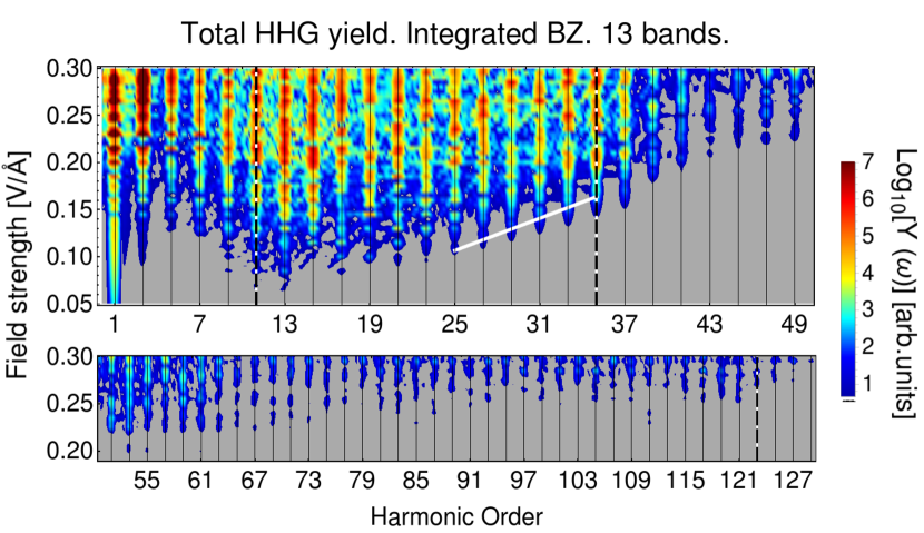
Figure 10: (Color online). As Fig. 9, but integrated over initial $k$-channels from the entire first BZ.

Above the $\approx$ 35th harmonic and at the highest field strengths shown in Figs. 9 and 10, a new plateau emerges, which we attribute to contributions from the second and third conduction band. If only the ${k=0}$ channel is included, the second plateau emerges at a higher field strength, $E_{0}>\pi\omega_{0}/a$, than in calculations including the entire first BZ. This field strength corresponds to the vector potential for which the cutoff frequency acquires its maximum value ${\omega^{c}(0,\,E_{0}/\omega_{0})=\Delta\varepsilon^{vc}_{max}}$ given by Eq. (37).

III.2.2 Field-strength dependence of the HHG cutoff

Figure 11 shows the field-strength dependence of the HHG cutoff we obtained from 13-band TDSE calculations by either including $\Gamma-$point-only emission (square markers) or $k$-channels from the entire first BZ (triangular markers), in comparison with the multi-band calculations from the literature. The solid blue line shows 51-band TDSE results for emission from the $\Gamma-$point-only, adapted from Fig. 3(a) in Ref. Wu et al. (2015). The orange dashed line shows HHG cutoff orders obtained by the direct propagation of the one-dimensional TDSE for $\Gamma-$point-only emission by Li et al.  Li et al. (2018b). The black dash-dotted line is adapted from the 6-band SBE calculation, including $k$-channels from the entire first BZ, of Li et al. .

For $\Gamma-$point only emission yields our stationary-phase approximation results in Fig. 11 (red dashed line) compare well with our 13-band calculations (square markers). Both are in reasonable agreement with the 51-band TDSE calculation of Wu et al.  Wu et al. (2015) (blue line). The cutoff harmonic orders we obtain in stationary-phase approximation are red-shifted by about three harmonic orders relative to the results of Li et al.  Li et al. (2018b) (orange dashed line), but approximately match the slope of the field-strength-dependent cutoff increase found by Li et al. . The cutoff harmonic orders predicted by our BZ-integrated 13-band calculation (triangular markers) agree well with our analytical stationary-phase approximation (green dotted line) and the 6-band SBE calculation of Li et al. (black dashed-dotted line). We note that the calculation of Li et al. includes a heuristic dephasing time, in contrast to our approach, where, apart from the adjusted potential strenghth of the Kronig-Penney model potential, no ad hoc parameters are introduced.

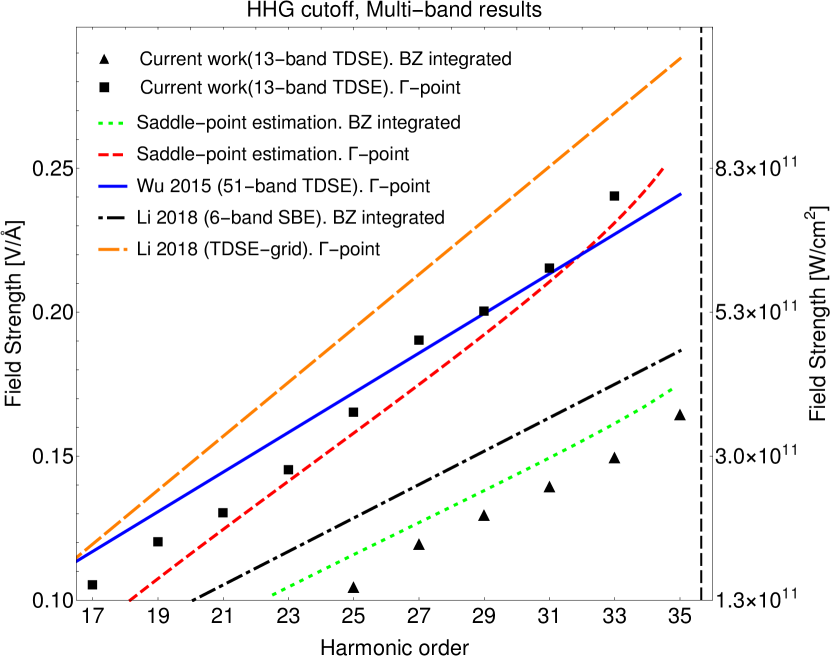
Figure 11: (Color online). Dependence of HHG-cutoff order on the peak laser-electric-field strength (left vertical axis) or intensity (right vertical axis) from calculation including more than two bands. Square markers show HHG cutoffs for $\Gamma-$point-only (${k=0}$) emission. Triangular markers indicate HHG cutoffs including $k$-channels from the entire first BZ. The blue solid line shows 51-band TDSE results for emission from the $\Gamma-$point-only, adapted from Fig. 3(a) in Ref. Wu et al. (2015). The black dotted and orange dashes lines are adapted from the BZ-integrated 4-band SBE calculation and the numerical TDSE solution for $\Gamma-$point-only emission by Li et al. . To facilitate the comparison with the 2-band cutoff calculations, we reproduce the saddle-point-approximation results of Fig. 7 (red dashed and green solid line).

IV Conclusions

We investigated intra- and interband HHG from a solid within the SAE approximation, based on a one-dimensional Kronig-Penney model of the solid’s electronic band structure. We expanded the active electron wavefunction in a basis of adiabatically field-dressed Bloch states (Houston states). We theoretically analyzed within a stationary-phase approximation and numerically evaluated in two-band calculations, contribution to the HHG yield from specific initial-state crystal momenta $k$ in the first BZ. This revealed essential contributions to the HHG yield from non-zero crystal momenta in the first BZ. We found complementary contributions to the HHG yield from intra- and interband emission. While intraband emission dominates below the threshold for interband excitation, interband emission almost exclusively determines the HHG yield above this threshold. Applying a stationary-phase approximation, we derived closed analytical expressions for the HHG yields and cutoff dependence on the laser-electric-field strength. This allow us, for example, to estimate the loss of accuracy in calculating HHG yields that are induced by restricting $k$ to a small interval near the $\Gamma-$point in the first BZ, as compared to BZ-integrated yields.

By adjusting the Kronig-Penney model potential to the published electronic-structure data for MgO crystals, we validated our theoretical analysis against numerically calculated $k$-resolved and $k$-integrated HHG yields and cutoff frequencies for a range of laser intensities. These analytical predictions and numerical calculations are in very good agreement with each other. They are also in qualitative and fair quantitative agreement with different numerical calculations from other authors. Investigating the characteristics of HHG for initial crystal momenta in the entire first BZ, we find significant HHG yields at even high-order harmonic orders for ${k\neq 0}$ (off the $\Gamma-$point). Even harmonics are particularly prominent for the lowest intraband harmonics. As observed experimentally and expected due to the symmetric dispersion of the model MgO solid with respect to the BZ-zone center, our BZ-integrated yields predominantly contain odd harmonics. In contrast to HHG in gaseous atoms, we confirm the cutoff harmonic order to increase linearly with the peak electric-field strength of the driving laser.

Our numerical calculations for MgO confirm our stationary-phase-approximation results that restraining the crystal momentum to an arbitrarily small range of crystal momenta close to the $\Gamma-$point does not adequately model HHG in solids driven by intense laser fields. Strongly depending on the laser intensity, in calculations with more than two bands, we find a second plateau above the cutoff HHG order we determined in two-band calculations.

Appendix A Kronig-Penney basis functions

The band structure of the Kronig-Penney model for periodic delta potentials,

$$V(x)=V_{0}\sum_{j}\delta(x-ja)\,,$$ (56)

is given by Eq. (3) of the main text and the eigenfunctions

$$\phi_{nk}(x) =|A_{nk}|\left[e^{i\alpha_{nk}\left(x-\frac{a}{2}\right)}\right.$$

$$\left.-\frac{1-e^{ia(\alpha_{nk}-k)}}{1-e^{-ia(\alpha_{nk}+k)}}e^{-i\alpha_{nk}\left(x+\frac{a}{2}\right)}\right]\,,$$

with the normalization factor

$$\left|A_{nk}\right|^{2}=\frac{\sin^{2}\left[a(\alpha_{nk}+k)/2\right]}{1-\frac{\sin(2a\alpha_{nk})}{2a\alpha_{nk}}-\cos(ak)\left[\cos(a\alpha_{nk})-\frac{\sin(a\alpha_{nk})}{a\alpha_{nk}}\right]}$$

and corresponding eigenenergies

$$\varepsilon_{nk}=\frac{\alpha_{nk}^{2}}{2}\,.$$ (57)

For crystal momenta ${k=0}$ and even $n$, and for ${k=\pi/a}$ and odd $n$, we have ${\alpha_{nk}=n\pi/a}$.

We adjust the global phase of the eigenfunctions to yield real matrix elements in Eq. (7) of the main text,

$$P^{nn^{\prime}}_{k}=\frac{2|A_{nk}||A_{n^{\prime}k}|\alpha_{nk}\alpha_{n^{\prime}k}\left[\cos(a\alpha_{n^{\prime}k})-\cos(a\alpha_{nk})\right]}{a\sin\left[\frac{a}{2}(\alpha_{nk}+k)\right]\sin\left[\frac{a}{2}(\alpha_{n^{\prime}k}+k)\right]\left(\alpha_{nk}^{2}-\alpha_{n^{\prime}k}^{2}\right)}$$

for ${n\neq n^{\prime}}$, and real diagonal matrix elements

$$P^{nn}_{k}=\frac{\alpha_{nk}\sin(a\alpha_{nk})\sin(ak)}{1-\frac{\sin(2a\alpha_{nk})}{2a\alpha_{nk}}-\cos(ak)\left[\cos(a\alpha_{nk})-\frac{\sin(a\alpha_{nk})}{a\alpha_{nk}}\right]}\,.$$

Appendix B Analytical continuation of the Kronig-Penney basis

In our analysis of the interband current, we extend the energies in Eq. (57) to the complex ${K-}$plane, defining ${K=k+ik_{i}}$, where ${k_{i}}$ is the imaginary part of the complex crystal momentum, and request

$$\lim_{k_{i}\to 0}\alpha_{nK}=\alpha_{nk}\;\;\;,{\lim_{k_{i}\to 0}\varepsilon_{nK}=\varepsilon_{nk}}\,.$$

Equation (3) and its $K$-derivative at ${K=0}$yield

$$1 =\cos(a\alpha_{n0})+\frac{V_{0}}{\alpha_{n0}}\sin(a\alpha_{n0})$$

$$0 =\left[\frac{a\,V_{0}\cos(a\alpha_{n0})}{\alpha_{n0}}-\left(a+\frac{V_{0}}{\alpha_{n0}^{2}}\right)\sin(a\alpha_{n0})\right]\frac{\text{d}\alpha_{n0}}{\text{d}K}.$$

After eliminating ${V_{0}}$ in these two equations, we see that the term in square brackets of the second equation cannot be zero, since ${2\pi\leq a\alpha_{n0}<3\pi}$ for ${n=v\,,c}$. This implies

$$\left.\frac{\text{d}\alpha_{nK}}{\text{d}K}\right|_{K=0}=0\;,\;\;\;\;n=v,\,c$$ (58)

and shows that

$$\left.\frac{\text{d}\left(\Delta\varepsilon_{K}^{cv}\right)}{\text{d}K}\right|_{K=0}=0\,.$$ (59)

From the second derivative of Eq. (3) with respect to $K$ and Eq. (58), we obtain

$$-a^{2}=\left[\frac{a\,V_{0}\cos(a\alpha_{n0})}{\alpha_{n0}}-\left(a+\frac{V_{0}}{\alpha_{n0}^{2}}\right)\sin(a\alpha_{n0})\right]\frac{\text{d}^{2}\alpha_{n0}}{\text{d}K^{2}}\,.$$

As noted in the main text, the coefficients in front of the second derivative are real. They do not vanish, since $2\pi\leq a\alpha_{n0}<3\pi$ for ${n=v\,,c}$. From this we conclude that

$$\Im\left[\left.\frac{\text{d}^{2}\alpha_{nK}}{\text{d}K^{2}}\right|_{K=0}\,\right]=0\;,\;\;\;\;n=v,\,c$$

and, consequently,

$$\Im\left[\left.\frac{\text{d}^{2}\left(\Delta\varepsilon^{cv}_{K}\right)}{\text{d}K^{2}}\right|_{K=0}\,\right]=0\,.$$

Appendix C Alternative expression for the interband current

We here derive the interband current in Eq. (18) of in the main text. Defining the function

$$\eta_{k}^{er}=\rho^{cv}_{k}(t)D^{vc}_{\kappa(t)}e^{-iS(k,\,t)}\,,$$ (60)

we employ Eq. (6) to obtain its derivative

$$\dot{\eta}_{k}^{er} =\dot{\rho}^{cv}_{k}(t)D^{vc}_{\kappa(t)}e^{-iS(k,\,t)}$$

$$+\rho^{cv}_{k}(t)\dot{D}^{vc}_{\kappa(t)}e^{-iS(k,\,t)}$$

$$-P^{vc}_{\kappa(t)}\rho^{cv}_{k}(t)\,e^{-iS(k,\,t)}\,.$$

Using ${\left(D^{vc}_{\kappa(t)}\right)^{2}=-\left|D^{vc}_{\kappa(t)}\right|^{2}}$ and substitution of ${\dot{\rho}^{cv}_{k}(t)}$ from Eq. (21) results in

$$-\rho^{cv}_{k}(t)P^{vc}_{\kappa(t)}e^{-iS(k,\,t)}= \dot{\eta}_{k}^{er}-i\Delta\rho_{k}^{vc}(t)E(t)\left|D^{vc}_{\kappa(t)}\right|^{2}$$

$$- \rho^{cv}_{k}(t)\dot{D}^{vc}_{\kappa(t)}e^{-iS(k,\,t)}\,.$$

Since the second term in this equation is purely imaginary, after replacing the ${\eta^{er}_{k}(t)}$ from Eq. (60), Eq. (17) can be written as

$$J^{er}_{k}(t)= \frac{d}{dt}\left[\rho^{cv}_{k}(t)D^{vc}_{\kappa(t)}e^{-iS(k,\,t)}\right]$$ (61)

$$-\rho^{cv}_{k}(t)\dot{D}^{vc}_{\kappa(t)}e^{-iS(k,\,t)}+\text{c.c.}\,.$$

Appendix D Saddle-point approximation for the $k$-channel interband yield

We evaluate the action in Eq. (36) by splitting its integral representation into two parts,

$$S(k,t_{s})=\int_{0}^{t_{0}}\Delta\varepsilon_{K(t)}^{cv}dt+\int_{t_{0}}^{t_{s}}\Delta\varepsilon_{K(t)}^{cv}dt\;,$$ (62)

with ${t_{0}=\Re[t_{s}]}$. Along the integration path illustrated in Fig. 12, the first integral is real.

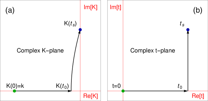
Figure 12: Contour integration for the action evaluation. (a) Integration path in the complex crystal-momentum ($K-$)plane, starting at ${K=k}$ (green dot), moving along the real $K-$axis to ${K(t_{0})}$, and arriving at the root of the analytic continuation of the band-gap energy ${\Delta\varepsilon_{K}^{cv}}$, ${K(t_{s})}$. (b) Corresponding path in the complex temporal plane, starting at time ${t=0}$ (green dot) and arriving at ${t_{s}}$ (blue dot).

To evaluate the second integral, we need to calculate ${t_{s}}$. For this purpose, we consider the continuum-wave vector potential ${A_{0}\sin(\omega_{0}t)}$, for which we find

$$t_{s}=\frac{1}{\omega_{0}}\arcsin\left[-k/A_{0}\pm i\gamma\right],$$ (63)

with

$$\gamma=\frac{\omega_{0}\sqrt{2\Delta\varepsilon_{0}^{cv}m^{*}_{0}}}{E_{0}}$$

and ${E_{0}=A_{0}\,\omega_{0}}$. For ${\gamma<1}$ and ${k<A_{0}<\pi/a}$, Taylor expansion of Eq. (63) results in

$$\Im[t_{s}]=\pm\frac{\gamma}{\omega_{0}\sqrt{1-(k/A_{0})^{2}}}+\mathcal{O}(\gamma^{3})\;,$$ (64)

which will be a fair approximation if ${\sqrt{1-(k/A_{0})^{2}}<\gamma}$.

We can now carry out the integrations in Eq. (62) and obtain

$$S(k,t_{s}) =\Re[S(k,\,t_{s})]+i\Delta\varepsilon_{0}^{cv}\Im[t_{s}]$$ (65)

$$+\frac{A^{2}}{8m^{*}_{0}}\left\{2\Im[t_{s}]-\sinh\left\{2\omega_{0}\Im[t_{s}]\right\}/\omega_{0}\right\}$$

$$+\frac{k^{2}}{2m^{*}_{0}}\left\{\Im[t_{s}]-\tanh\left[\omega_{0}\Im[t_{s}]\right\}/\omega_{0}\right\}\,,$$

where

$$\Re[S(k,t_{s})]=\int_{0}^{t_{0}}\Delta\varepsilon_{K(t)}^{cv}dt+\Re\left[\int_{t_{0}}^{t_{s}}\Delta\varepsilon_{K(t)}^{cv}dt\right]\;.$$

To find the pre-exponential factor in Eq. (36), we first point out that the cross derivatives ${\partial^{2}\sigma_{\omega}(k,\,t,\,t^{\prime})/\partial t\partial t^{\prime}}$ and ${\partial^{2}\sigma_{\omega}(k,\,t,\,t^{\prime})/\partial t^{\prime}\partial t}$ vanish, such that

$$\left|\text{det Hess}\right| =\left|\frac{\partial^{2}\sigma_{\omega}(k,\,t_{e},\,t_{s})}{\partial t^{\prime}\,{}^{2}}\frac{\partial^{2}\sigma_{\omega}(k,\,t_{e},\,t_{s})}{\partial t^{2}}\right|$$

$$=\left|E(t_{s})\sqrt{\frac{2\Delta\varepsilon_{0}^{cv}}{m^{*}_{0}}}E(t_{e})\left(P^{cc}_{\kappa(t_{e})}-P^{vv}_{\kappa(t_{e})}\right)\right|\;.$$

Following Milos̆evic et al. (2002); Lewenstein et al. (1994), only keeping the regular solution in Eq. (64), ${\Im[t_{s}]>0}$, we obtain

$$\hat{\bar{J}}^{er}_{k}(\omega) \approx-\left(2\pi\omega\right)\left|D^{vc}_{0}\right|^{2}e^{-\Im[S(k,\,t_{s})]}$$

$$\times\sum_{t_{e}}\frac{i\,E(t_{s})e^{-i\omega t_{e}}e^{i\Re[S(k,\,t_{s})]}e^{iS(k,\,t_{e})}}{\left|E(t_{s})\sqrt{\frac{2\Delta\varepsilon_{0}^{cv}}{m^{*}_{0}}}E(t_{e})\left(P^{cc}_{\kappa(t_{e})}-P^{vv}_{\kappa(t_{e})}\right)\right|^{1/2}}.$$

The interband HHG yield is thus given by

$$Y^{er}_{k}(\omega) \approx\left(2\pi\omega\right)^{2}e^{-2\Im[S(k,\,t_{s})]}\left|D^{vc}_{0}\right|^{4}E(t_{s})\sqrt{\frac{m^{*}_{0}}{2\Delta\varepsilon_{0}^{cv}}}$$

$$\times\left|\sum_{t_{e}}\frac{e^{-i\omega t_{e}}\left[e^{i\left\{\Re[S(k,\,t_{s})]+S(k,\,t_{e})+\frac{\pi}{2}\right\}}+\text{c.c.}\right]}{\left|E(t_{e})\left(P^{cc}_{\kappa(t_{e})}-P^{vv}_{\kappa(t_{e})}\right)\right|^{1/2}}\right|^{2}\;.$$

In order to get a more explicit equation in terms of the band and laser field parameters, we approximate ${E(t_{s})}$ to first order in $\gamma$,

$$E(t_{s})\approx E_{0}\sqrt{1-(k/A_{0})^{2}}+\mathcal{O}(\gamma^{2})\;,$$ (66)

and apply the approximations used to derive ${\Im[S(k,\,t_{s})]}$ in Eq. (65). This leads to the interband yield

$$Y^{er}_{k}(\omega) \approx\exp\left[-\frac{2\,\sqrt{2m^{*}_{0}}\,{\Delta\varepsilon_{0}^{cv}}^{3/2}}{E_{0}\sqrt{1-(k/A_{0})^{2}}}\right]$$

$$\times\left(2\pi\omega\right)^{2}\left|D^{vc}_{0}\right|^{4}E_{0}\sqrt{1-(k/A_{0})^{2}}\sqrt{\frac{m^{*}_{0}}{2\Delta\varepsilon_{0}^{cv}}}$$

$$\times\left|\sum_{t_{e}}\frac{e^{-i\omega t_{e}}\left[e^{i\left\{\Re[S(k,\,t_{s})]+S(k,\,t_{e})+\frac{\pi}{2}\right\}}+\text{c.c.}\right]}{\left|E(t_{e})\left(P^{cc}_{\kappa(t_{e})}-P^{vv}_{\kappa(t_{e})}\right)\right|^{1/2}}\right|^{2}\;.$$

Appendix E Simplification of Eq. (48)

We here approximate Eq. (48), proceeding in a similar way as in Appendix D, by splitting Eq. (48) in a real and a complex integral (Fig. 12)

$$\int_{t_{s}}^{t_{e}}\Delta P^{vc}_{\kappa_{r}(t)}dt=I_{1}+I_{2}\,,$$

with

$$I_{1} =\int_{t_{s}}^{t_{0}}\Delta P^{vc}_{\kappa_{r}(t)}dt$$

$$I_{2} =\int_{t_{0}}^{t_{e}}\Delta P^{vc}_{\kappa_{r}(t)}dt\,.$$

Following the derivation of Eq. (38), we find

$$\frac{d\left(\varepsilon^{cv}_{K}\right)}{dK}\equiv-\Delta P^{vc}_{K}=\frac{K}{m^{*}_{0}}+\mathcal{O}(K^{3})\,.$$

Using ${\kappa(t)=k+A(t)}$, we perform the integral in $I_{1}$ by contour integration in the complex plane to obtain

$$I_{1} =\frac{k}{i\omega_{0}m_{0}^{*}}\left\{\tanh\left[\omega_{0}\Im(t_{s})\right]-\omega_{0}\Im(t_{s})\right\}$$

$$-\frac{A_{0}}{\omega_{0}m_{0}^{*}}\cos(\omega_{0}t_{0})\left\{1-\cosh\left[\omega_{0}\Im(t_{s})\right]\right\}$$

$$\approx\mathcal{O}(\gamma^{3})\;,$$

where we used that, according Eq. (38), ${K(t_{s})}$ is imaginary. Thus, to second order in $\gamma$, ${I_{1}\approx 0}$ and Eq. (48) can be approximated as the real integral

$$\int_{t_{s}}^{t_{e}}\Delta P^{vc}_{\kappa_{r}(t)}dt\approx\int_{t_{0}}^{t_{e}}\Delta P^{vc}_{\kappa_{r}(t)}dt\,.$$

This expression is more suitable for numerical calculations than Eq. (48).

References

- Le et al. (2009) A.-T. Le, R. R. Lucchese, S. Tonzani, T. Morishita, and C. D. Lin, Phys. Rev. A 80, 013401 (2009).
- Krausz and Ivanov (2009) F. Krausz and M. Ivanov, Rev. Mod. Phys. 81, 163 (2009).
- Plaja and Roso-Franco (1992) L. Plaja and L. Roso-Franco, Phys. Rev. B 45, 8334 (1992).
- Protopapas et al. (1997) M. Protopapas, C. H. Keitel, and P. L. Knight, Rep. Progr. Phys. 60, 389 (1997).
- Faisal and Kamiński (1996) F. H. M. Faisal and J. Z. Kamiński, Phys. Rev. A 54, R1769 (1996).
- Faisal and Kaminski (1997) F. H. M. Faisal and J. Z. Kaminski, Phys. Rev. A 56, 748 (1997).
- Ghimire et al. (2011) S. Ghimire, A. D. DiChiara, E. Sistrunk, P. Agostini, L. F. DiMauro, and D. A. Reis, Nat. Phys. 7, 138 (2011).
- Wu et al. (2015) M. Wu, S. Ghimire, D. A. Reis, K. J. Schafer, and M. B. Gaarde, Phys. Rev. A 91, 043839 (2015).
- Vampa et al. (2014) G. Vampa, C. R. McDonald, G. Orlando, D. D. Klug, P. B. Corkum, and T. Brabec, Phys. Rev. Lett. 113, 073901 (2014).
- Li et al. (2016) J. Li, E. Saydanzad, and U. Thumm, Phys. Rev. A 94, 051401 (2016).
- Li et al. (2017) J. Li, E. Saydanzad, and U. Thumm, Phys. Rev. A 95, 043423 (2017).
- Li et al. (2018a) J. Li, E. Saydanzad, and U. Thumm, Phys. Rev. Lett. 120, 223903 (2018a).
- Leone et al. (2014) S. R. Leone, C. W. McCurdy, J. Burgdörfer, L. S. Cederbaum, Z. Chang, N. Dudovich, J. Feist, C. H. Greene, M. Ivanov, R. Kienberger, U. Keller, M. F. Kling, Z.-H. Loh, T. Pfeifer, A. N. Pfeiffer, R. Santra, K. Schafer, A. Stolow, U. Thumm, and M. J. J. Vrakking, Nat. Photonics 8, 162 EP (2014).
- Thumm et al. (2015) U. Thumm, Q. Liao, E. M. Bothschafter, F. Süßmann, M. F. Kling, and R. Kienberger, “Attosecond physics: Attosecond streaking spectroscopy of atoms and solids,” in Photonics (John Wiley & Sons, Ltd, 2015) Chap. 13, pp. 387–441.
- Ciappina et al. (2017) M. F. Ciappina, J. A. Pérez-Hernández, A. S. Landsman, W. A. Okell, S. Zherebtsov, B. Förg, J. Schötz, L. Seiffert, T. Fennel, T. Shaaran, T. Zimmermann, A. Chacón, R. Guichard, A. Zaïr, J. W. G. Tisch, J. P. Marangos, T. Witting, A. Braun, S. A. Maier, L. Roso, M. Krüger, P. Hommelhoff, M. F. Kling, F. Krausz, and M. Lewenstein, Rep. Progr. Phys. 80, 054401 (2017).
- Kruchinin et al. (2018) S. Y. Kruchinin, F. Krausz, and V. S. Yakovlev, Rev. Mod. Phys. 90, 021002 (2018).
- Luu and Wörner (2016) T. T. Luu and H. J. Wörner, Phys. Rev. B 94, 115164 (2016).
- Ghimire and Reis (2019) S. Ghimire and D. Reis, Nat. Phys. 15, 10 (2019).
- Ndabashimiye et al. (2016) G. Ndabashimiye, S. Ghimire, M. Wu, D. A. Browne, K. J. Schafer, M. B. Gaarde, and D. A. Reis, Nature 534, 520 EP (2016).
- Vampa et al. (2015) G. Vampa, C. R. McDonald, G. Orlando, P. B. Corkum, and T. Brabec, Phys. Rev. B 91, 064302 (2015).
- Osika et al. (2017) E. N. Osika, A. Chacón, L. Ortmann, N. Suárez, J. A. Pérez-Hernández, B. Szafran, M. F. Ciappina, F. Sols, A. S. Landsman, and M. Lewenstein, Phys. Rev. X 7, 021017 (2017).
- Li et al. (2018b) J. Li, S. Fu, H. Wang, X. Zhang, B. Ding, B. Hu, and H. Du, Phys. Rev. A 98, 043409 (2018b).
- Mücke (2011) O. D. Mücke, Phys. Rev. B 84, 081202 (2011).
- Hawkins et al. (2015) P. G. Hawkins, M. Y. Ivanov, and V. S. Yakovlev, Phys. Rev. A 91, 013405 (2015).
- Golde et al. (2008) D. Golde, T. Meier, and S. W. Koch, Phys. Rev. B 77, 075330 (2008).
- Schubert et al. (2014) O. Schubert, M. Hohenleutner, F. Langer, B. Urbanek, C. Lange, U. Huttner, D. Golde, T. Meier, M. Kira, S. W. Koch, and R. R. Huber, Nat. Photonics 8, 147 (2014).
- Meier et al. (1994) T. Meier, G. von Plessen, P. Thomas, and S. W. Koch, Phys. Rev. Lett. 73, 902 (1994).
- Jiang et al. (2017) S. Jiang, H. Wei, J. Chen, C. Yu, R. Lu, and C. D. Lin, Phys. Rev. A 96, 053850 (2017).
- Jiang et al. (2018) S. Jiang, J. Chen, H. Wei, C. Yu, R. Lu, and C. D. Lin, Phys. Rev. Lett. 120, 253201 (2018).
- Korbman et al. (2013) M. Korbman, S. Yu, and V. S. Yakovlev, New. J. Phys. 15, 013006 (2013).
- Krieger and Iafrate (1985) J. B. Krieger and G. J. Iafrate, Phys. Rev. B 33, 5494 (1985).
- Haug and Koch (1998) H. Haug and S. Koch, Theory of Transport Properties of Semiconductor Nanostructures (Springer Science+Business Media Dordrecht, 1998).
- Lindefelt et al. (2004) U. Lindefelt, H.-E. Nilsson, and M. Hjelm, Semicond. Sci. Technol. 19, 1061 (2004).
- Kronig et al. (1931) R. D. L. Kronig, W. G. Penney, and R. H. Fowler, Proc. Royal Soc. Lond. A 130, 499 (1931).
- Atkins and Friedman (2005) P. Atkins and R. Friedman (Oxford University Press, Oxford, 2005).
- Ashcroft and Mermin (1976) N. W. Ashcroft and N. D. Mermin, Solid State Physics (Halcourt College Publishers, United States, 1976).
- Keldysh (1965) L. V. Keldysh, JETP 20, 1307 (1965).
- Lewenstein et al. (1994) M. Lewenstein, P. Balcou, M. Y. Ivanov, A. L’Huillier, and P. B. Corkum, Phys. Rev. A 49, 2117 (1994).
- Wong (2001) R. Wong, Asymptotic Approximations of Integrals, Vol. 34 (Society for Industrial and Applied Mathematics., Philadelphia, PA, USA, 2001).
- Xu and Ching (1991) Y.-N. Xu and W. Y. Ching, Phys. Rev. B 43, 4461 (1991).
- Ghimire et al. (2012) S. Ghimire, A. D. DiChiara, E. Sistrunk, G. Ndabashimiye, U. B. Szafruga, A. Mohammad, P. Agostini, L. F. DiMauro, and D. A. Reis, Phys. Rev. A 85, 043836 (2012).
- Milos̆evic et al. (2002) D. B. Milos̆evic, G. G. Paulus, and W. Becker, Phys. Rev. Lett 89, 153001 (2002).