July 25, 2019

Precision calculations of $B\to V$ form factors in QCD

Jing Gao^a,b, Cai-Dian Lü^a,b, Yue-Long Shen^c, Yu-Ming Wang^d, Yan-Bing Wei^d

^a   Institute of High Energy Physics, CAS, P.O. Box 918(4) Beijing 100049, China
^b   School of Physics, University of Chinese Academy of Sciences, Beijing 100049, China
^c   College of Information Science and Engineering, Ocean University of China, Songling Road 238, Qingdao, 266100 Shandong, P.R. China
^d School of Physics, Nankai University, 300071 Tianjin, China  

Applying the vacuum-to-$B$-meson correlation functions with an interpolating current for the light vector meson we construct the light-cone sum rules (LCSR) for the “effective” form factors $\xi_{\parallel}(n\cdot p)$, $\xi_{\perp}(n\cdot p)$, $\Xi_{\parallel}(\tau,n\cdot p)$ and $\Xi_{\perp}(\tau,n\cdot p)$, defined by the corresponding hadronic matrix elements in soft-collinear effective theory (SCET), entering the leading-power factorization formulae for QCD form factors responsible for $B\to V\ell\bar{\nu}_{\ell}$ and $B\to V\ell\bar{\ell}$ decays at large hadronic recoil at next-to-leading-order in QCD. The evanescent-operator approach for the perturbative matching of the effective operators from $\rm{SCET_{I}}\to{HQET}$ is employed in the determination of the hard-collinear functions entering the SCET factorization formulae for the vacuum-to-$B$-meson correlation functions. The light-quark mass effect for the local SCET form factors $\xi_{\parallel}(n\cdot p)$ and $\xi_{\perp}(n\cdot p)$ is also computed from the LCSR method with the $B$-meson light-cone distribution amplitude $\phi_{B}^{+}(\omega,\mu)$ at ${\cal O}(\alpha_{s})$. Furthermore, the subleading power corrections to $B\to V$ form factors from the higher-twist $B$-meson light-cone distribution amplitudes are also computed with the same method at tree level up to the twist-six accuracy. Employing the two different models for the $B$-meson light-cone distribution amplitudes consistent with QCD equations of motion, we observe that the higher-twist corrections to $B\to V$ form factors are dominated by the two-particle twist-five distribution amplitude $g_{B}^{-}(\omega,\mu)$, in analogy to the previous observation for $B\to P$ form factors. Having at our disposal the LCSR predictions for $B\to V$ form factors, we further perform new determinations of the CKM matrix element $|V_{ub}|$ from the semileptonic $B\to\rho\,\ell\,\bar{\nu}_{\ell}$ and $B\to\omega\,\ell\,\bar{\nu}_{\ell}$ decays, and predict the normalized differential branching fractions and the $q^{2}$-binned $K^{\ast}$ longitudinal polarization fractions of the exclusive rare $B\to K^{\ast}\,\nu_{\ell}\,\bar{\nu}_{\ell}$ decays.

1 Introduction

Precision calculations of $B\to V$ form factors are indispensable for the determinations of the CKM matrix elements from the semileptonic $B\to V\,\ell\,\bar{\nu}_{\ell}$ decays and the radiative penguin $B\to V\gamma$ decays and for the theory descriptions of the electroweak penguin $B\to V\ell\bar{\ell}$ decays as well as the hadronic two-body $B$-meson decays in QCD. In the low hadronic recoil region, the unquenched lattice QCD calculations of $B\to K^{\ast}$ form factors have been performed [1, 2] (see references therein for discussions on the earlier calculations with the quenched approximation) by employing the MILC Collaboration gauge-field ensembles with an improved staggered quark action [3]. In the large hadronic recoil region, distinct analytical QCD methods have been developed for the systematic calculations of the heavy-to-light $B$-meson decay form factors with the aid of the heavy quark expansion.

QCD factorization formulae for heavy-to-light form factors at large recoil were originally proposed in [4] at leading power in $\Lambda/m_{Q}$, where both the soft contribution satisfying the large-recoil symmetry relations and the hard spectator scattering effect violating the symmetry relations were shown to appear simultaneously in contrast to the hard-collinear factorization for the pion-photon form factor. With the advent of soft-collinear effective theory (SCET) factorization properties of heavy-to-light form factors can be addressed by integrating out the hard and hard-collinear fluctuations of the QCD matrix elements one after the other. Implementing the first-step matching procedure for the QCD current $\bar{\psi}\,\Gamma_{i}\,Q$ will give rise to the so-called ${\rm A0}$-type and ${\rm B1}$-type ${\rm SCET}_{\rm I}$ operators [5, 6, 7], both of which can contribute to heavy-to-light form factors at leading power in $\Lambda/m_{Q}$. Performing the perturbative matching of the effective currents from ${\rm SCET}_{\rm I}\to{\rm SCET}_{\rm II}$ indicates that the soft-collinear factorization for the ${\rm A0}$-type matrix elements cannot be achieved, due to the emergence of end-point divergences appearing in the convolution integrals of the hard-collinear functions and the light-cone distribution amplitudes. By contrast, the non-local form factors defined by the ${\rm B1}$-type ${\rm SCET}_{\rm I}$ operators can be further expressed as the convolution of the jet functions and the hadronic distribution amplitudes [7]. It is then evident that the theory predictions of heavy-to-light form factors from the SCET factorization formulae cannot be made without the knowledge of the standard light-cone distribution amplitudes and the matrix elements of the ${\rm A0}$-type ${\rm SCET}_{\rm I}$ operators.

Applying the dispersion relations and perturbative QCD factorization theorems for the vacuum-to-vector-meson correlation functions, the QCD light-cone sum rules (LCSR) for $B\to V$ form factors can be readily constructed [8, 9, 10, 11] with the parton-hadron duality ansatz and the narrow-width approximation for the vector mesons (see [12, 13, 14] for further discussions and [15] for the sum-rule construction with the helicity form-factor scheme). Alternatively, the QCD LCSR for heavy-to-light $B$-meson decay form factors can be derived from the vacuum-to-$B$-meson correlation functions, following the analogous strategies, at leading order (LO) [16, 17, 18, 19] and next-to-leading order (NLO) [20, 21, 22] in the strong coupling $\alpha_{s}$, where the factorization formulae for the correlation functions under discussion were established with the diagrammatic approach and the strategy of regions [23, 24]. Constructing the LCSR for the ${\rm SCET}_{\rm I}$ matrix elements entering the QCD factorization formulae of heavy-to-light $B$-meson decay form factors has been achieved in [25, 26] employing the vacuum-to-$B$-meson correlation functions. Compared to the QCD factorization approach, the LCSR calculations of heavy-to-light $B$-meson form factors depend on the duality assumption of either the light-meson channel or the $B$-meson channel.

Yet another factorization approach to compute heavy-to-light $B$-meson form factors at large recoil has been developed to regularize the rapidity divergences of the ${\rm A0}$-type SCET matrix elements by the intrinsic transverse momenta of the soft and collinear partons involved in the hard scattering processes [27, 28]. Perturbative QCD corrections to the short-distance matching coefficient functions entering the transverse-momentum-dependent (TMD) factorization formulae of several hard exclusive processes of phenomenological interest [29, 30, 31] have been accomplished at leading-twist accuracy. The Sudakov and threshold resummation of enhanced logarithms entering the TMD wavefunctions have been performed for the $B$-meson [32] and for the pion [33] with the Collins-Soper-Sterman (CSS) formalism [34, 35, 36]. In addition, constructing the factorization-compatible definitions of the TMD wavefunctions free of the rapidity pinch singularities has been discussed in [37, 38], where the non-dipolar off-light-cone Wilson lines were introduced in the unsubtracted TMD pion wavefunctions to reduce the soft subtraction functions. However, a definite power counting scheme for all the momentum modes involved in the exclusive $B$-meson decays still needs to be constructed for the TMD factorization approach to clarify the conceptual differences between the perturbative QCD (PQCD) framework [27, 28] and the QCD factorization approach [4, 7] and to develop the TMD factorization for hard exclusive processes into a systematic theoretical framework.

Applying the SCET factorization for the QCD $B\to V$ form factors at large recoil, we aim at computing the hadronic matrix elements of both the ${\rm A0}$-type and ${\rm B}$-type ${\rm SCET}_{\rm I}$ operators by constructing the corresponding sum rules from the vacuum-to-$B$-meson correlation functions, in analogy to the prescriptions developed in [25, 26]. The major new improvements of the present paper can be summarized as follows.

• We establish the factorization formulae of the vacuum-to-$B$-meson correlation functions defined with an interpolating current for the vector meson and an effective weak current in ${\rm SCET}_{\rm I}$ at one loop using the evanescent approach [39, 40], instead of substituting the light-cone projector of the $B$-meson for evaluating the corresponding ${\rm SCET}_{\rm I}$ diagrams prior to performing the loop-momentum integration. In addition, QCD resummation of enhanced logarithms of $m_{b}/\Lambda$ entering the ${\rm A0}$-type and ${\rm B}$-type hard matching coefficients for the weak current $\bar{\psi}\,\Gamma_{i}\,Q$ is accomplished at next-to-leading-logarithmic (NLL) and leading-logarithmic (LL) accuracy with the standard renormalization-group (RG) formalism [41, 42].

• Applying the SCET representations of the vacuum-to-$B$-meson correlation functions in the presence of the subleading-power Lagrangian ${\cal L}_{\xi m}^{(1)}$, we construct the sum rules for the light-quark mass contributions to the ${\rm A0}$-type SCET form factors at tree level with the power counting scheme $m\sim\Lambda$. We demonstrate explicitly that the flavour SU(3)-symmetry breaking effects for the longitudinal vector meson form factors are not suppressed by powers of $\Lambda/m_{b}$ and evidently preserve the large recoil symmetry relations for the soft contributions to the semileptonic $B\to V$ form factors.

• We compute the subleading power corrections to $B\to V$ form factors from the higher-twist $B$-meson light-cone distribution amplitudes (LCDA) with the aid of the LCSR technique up to the twist-six accuracy. In particular, we employ a complete parametrization of the light-ray matrix element $\langle 0|\bar{q}_{\alpha}(z_{1}\,\bar{n})\,g_{s}\,G_{\mu\nu}(z_{2}\,\bar{n})\,h_{v\,\beta}(0)|\bar{B}_{v}\rangle$ in heavy-quark effective theory (HQET) defining eight independent invariant functions presented in [43] instead of four three-particle distribution amplitudes proposed in [44] in the light-cone limit. In an attempt to understand the systematic uncertainty of the LCSR predictions for $B\to V$ form factors, we apply two distinct models for the two-particle and three-particle $B$-meson LCDA, satisfying the classical QCD equations of motion and the corresponding asymptotic behaviours at small quark and gluon momenta determined by the conformal spins of the soft fields, as constructed in [43, 22].

• For the sake of understanding the long-standing discrepancy of the form-factor ratio ${\cal R}_{1}=\left[{(m_{B}+m_{V})/m_{B}}\right]\,T_{1}(q^{2})/V(q^{2})$ predicted by the QCD sum rule technique with the vector-meson LCDA [10] and by the QCD factorization approach [4, 42, 45], we carry out a detailed comparison of the various terms contributing to the factorization formula of the ratio ${\cal R}_{1}$ with their counterparts in the framework of the LCSR with the $B$-meson distribution amplitudes and identify the dominating QCD mechanisms responsible for the above-mentioned discrepancy.

The outline of this paper is as follows. We will review the ${\rm SCET(hc,c,s)}$ representations of $B\to V$ form factors at large hadronic recoil from integrating out the hard-scale fluctuations, which express the seven QCD form factors in terms of the four ${\rm SCET}_{\rm I}$ matrix elements, $\xi_{a}(n\cdot p)$ and $\Xi_{a}(\tau,n\cdot p)$ (with $a=\parallel,\perp$), as well as the perturbatively calculable short-distance coefficients at leading power in $\Lambda/m_{b}$ in section 2. Constructing the SCET sum rules for these “effective” form factors with the $B$-meson distribution amplitudes at leading twist accuracy will be presented in section 3 with a detailed demonstration of the factorization formulae for the vacuum-to-$B$-meson correlation functions at NLO in $\alpha_{s}$, where we pay particular attention to the infrared subtractions for deriving the master formulae of the hard-collinear matching functions in the presence of the evanescent operators. We proceed to compute the subleading power corrections to $B\to V$ form factors from both the two-particle and three-particle higher-twist $B$-meson LCDA with the LCSR method at tree level up to the twist-six accuracy in section 4, where the operator identities between the two-body and three-body light-ray HQET operators at classical level are employed to reduce the resulting sum rules. Phenomenological aspects of the newly derived LCSR for $B\to V$ form factors will be explored in section 5, including the numerical impacts of the subleading-power corrections in the heavy-quark expansion, an exploratory comparison of our predictions of the form-factor ratios with the SCET factorization calculations, the extrapolations of our results toward large momentum transfer with the $z$-series parametrization, the exclusive determinations of the CKM matrix elements $|V_{ub}|$ from the partial branching fractions of $B\to\rho\,\ell\,\bar{\nu}_{\ell}$ and $B\to\omega\,\ell\,\bar{\nu}_{\ell}$, and the $q^{2}$-binned distributions of the branching fractions as well as the $K^{\ast}$ longitudinal polarized fractions of the flavour-changing-neutral-current (FCNC) induced $B\to K^{\ast}\,\nu_{\ell}\,\bar{\nu}_{\ell}$ decays. A summary of our main observations and concluding remarks on the future development will be displayed in section 6. We further collect the explicit expressions for the ${\rm A0}$-type and ${\rm B}$-type hard functions from matching the QCD weak current $\bar{\psi}\,\Gamma_{i}\,Q$ onto ${\rm SCET}_{\rm I}$ at NLO and LO in $\alpha_{s}$, respectively, in Appendix A. Two phenomenological models for the two-particle and three-particle $B$-meson distribution amplitudes, up to the twist-six accuracy, employed in the numerical computations of the semileptonic $B\to V$ form factors are collected in Appendix B.

2 QCD factorization for $B\to V$ form factors

The purpose of this section is, following closely [41, 46, 42], to summarize the soft-collinear factorization formulae for $B\to V$ form factors at large hadronic recoil in ${\rm SCET}_{\rm I}$ by integrating out the strong interaction dynamics at the hard scale $m_{b}$, for the sake of establishing the theoretical framework for computing the SCET matrix elements from the LCSR method. The resulting ${\rm SCET(hc,c,s)}$ representations for the QCD heavy-to-light form factors are given by [7, 47, 5]

$$F^{B\to V}_{i}(n\cdot p)=C_{i}^{\rm(A0)}(n\cdot p)\,\xi_{a}(n\cdot p)+\int d\tau\,C_{i}^{\rm(B1)}(\tau,n\cdot p)\,\Xi_{a}(\tau,n\cdot p)\,,\,\,\,(a\,=\,\parallel,\,\,\perp)\,,$$ (1)

where the seven $B\to V$ form factors are expressed in terms of the four “effective” form factors in ${\rm SCET_{I}}$ at leading power in the heavy quark expansion. The hard matching coefficients for both the ${\rm A0}$-type and ${\rm B1}$-type SCET currents have been computed at one-loop accuracy [41, 48, 49]. As we aim at computing the semileptonic $B\to V$ form factors with the aid of the factorization formula (1) at ${\cal O}(\alpha_{s})$, we will need the perturbative matching functions $C_{i}^{\rm(A0)}(n\cdot p)$ at NLO in QCD and the ${\rm B1}$-type hard functions $C_{i}^{\rm(B1)}(\tau,n\cdot p)$ at tree level as displayed in Appendix A. The “effective” form factors $\xi_{a}(n\cdot p)$ and $\Xi_{a}(\tau,n\cdot p)$ are defined by the hadronic matrix elements of the corresponding ${\rm SCET_{I}}$ operators [42]

$$\langle V(p,\epsilon^{\ast})|\left(\bar{\xi}\,W_{c}\right)\,\gamma_{5}\,h_{v}\,|\bar{B}_{v}\rangle=-n\cdot p\,(\epsilon^{\ast}\cdot v)\,\xi_{\parallel}(n\cdot p)\,,$$

$$\langle V(p,\epsilon^{\ast})|\left(\bar{\xi}\,W_{c}\right)\,\gamma_{5}\,\gamma_{\mu\perp}\,h_{v}\,|\bar{B}_{v}\rangle=-n\cdot p\,(\epsilon^{\ast}_{\mu}-\epsilon^{\ast}\cdot v\,\bar{n}_{\mu})\,\xi_{\perp}(n\cdot p)\,,$$

$$\langle V(p,\epsilon^{\ast})|\left(\bar{\xi}\,W_{c}\right)\,\gamma_{5}\,\left(W_{c}^{\dagger}\,\,i\,\not\!\!D_{c\perp}\,W_{c}\right)(rn)\,h_{v}\,|\bar{B}_{v}\rangle=-n\cdot p\,m_{b}\,\epsilon^{\ast}\cdot v\,\int_{0}^{1}\,d\tau\,e^{i\,\tau\,n\cdot p\,r}\,\Xi_{\parallel}(\tau,\,n\cdot p)\,,$$

$$\langle V(p,\epsilon^{\ast})|\left(\bar{\xi}\,W_{c}\right)\,\gamma_{5}\,\gamma_{\mu\perp}\,\left(W_{c}^{\dagger}\,\,i\,\not\!\!D_{c\perp}\,W_{c}\right)(rn)\,h_{v}\,|\bar{B}_{v}\rangle$$

$$=-n\cdot p\,m_{b}\,(\epsilon^{\ast}_{\mu}-\epsilon^{\ast}\cdot v\,\bar{n}_{\mu})\,\int_{0}^{1}\,d\tau\,e^{i\,\tau\,n\cdot p\,r}\,\Xi_{\perp}(\tau,\,n\cdot p)\,,$$ (2)

where the light-cone Wilson line is introduced to restore the collinear gauge invariance [7, 50]

$$W_{c}(x)={\rm P}\,{\rm exp}\,\left[i\,g_{s}\,\int_{-\infty}^{0}\,ds\,n\cdot A_{c}(x+s\,n)\right]\,.$$ (3)

The QCD matrix elements of the heavy-to-light currents $\bar{\psi}\,\Gamma_{i}\,Q$ are parameterized by the semileptonic $B\to V$ form factors in the standard way [4]

$$c_{V}\,\langle V(p,\epsilon^{\ast})|\bar{q}\,\gamma_{\mu}\,b|\bar{B}(p+q)\rangle=-{2\,i\,V(q^{2})\over m_{B}+m_{V}}\,\epsilon_{\mu\nu\rho\sigma}\,\epsilon^{\ast\,\nu}\,p^{\rho}\,q^{\sigma}\,,$$

$$c_{V}\,\langle V(p,\epsilon^{\ast})|\bar{q}\,\gamma_{\mu}\,\gamma_{5}\,b|\bar{B}(p+q)\rangle={2\,m_{V}\,\epsilon^{\ast}\cdot q\over q^{2}}\,q_{\mu}\,A_{0}(q^{2})$$

$$\hskip 156.49014pt+(m_{B}+m_{V})\,\left[\epsilon^{\ast}_{\mu}-{\epsilon^{\ast}\cdot q\over q^{2}}\,q_{\mu}\right]\,A_{1}(q^{2})$$

$$\hskip 156.49014pt-{\epsilon^{\ast}\cdot q\over m_{B}+m_{V}}\,\left[(2\,p+q)_{\mu}-{m_{B}^{2}-m_{V}^{2}\over q^{2}}\,q_{\mu}\right]\,A_{2}(q^{2})\,,$$

$$c_{V}\,\langle V(p,\epsilon^{\ast})|\bar{q}\,i\,\sigma_{\mu\nu}\,q^{\nu}\,b|\bar{B}(p+q)\rangle=2\,i\,T_{1}(q^{2})\,\epsilon_{\mu\nu\rho\sigma}\,\epsilon^{\ast\,\nu}\,p^{\rho}\,q^{\sigma}\,,$$

$$c_{V}\,\langle V(p,\epsilon^{\ast})|\bar{q}\,i\,\sigma_{\mu\nu}\,\gamma_{5}\,q^{\nu}\,b|\bar{B}(p+q)\rangle=T_{2}(q^{2})\,\left[(m_{B}^{2}-m_{V}^{2})\,\epsilon^{\ast}_{\mu}-(\epsilon^{\ast}\cdot q)\,(2\,p+q)_{\mu}\right]$$

$$\hskip 184.9429pt+\,T_{3}(q^{2})\,(\epsilon^{\ast}\cdot q)\,\left[q_{\mu}-{q^{2}\over m_{B}^{2}-m_{V}^{2}}\,(2\,p+q)_{\mu}\right],$$ (4)

with the convention $\epsilon_{0123}=-1$. We have introduced the factor $c_{V}$ to account for the flavour structure of vector mesons with $c_{V}=\pm\sqrt{2}$ for the $\rho^{0}$ and $\omega$ (obviously, $\sqrt{2}$ for $b\to u$ transition and $-\sqrt{2}$ for the $b\to d$ transition) and $c_{V}=1$ otherwise. At maximal hadronic recoil $q^{2}=0$ there exist two relations for the above-mentioned $B\to V$ form factors in QCD

$${m_{B}+m_{V}\over 2\,m_{V}}\,A_{1}(0)-{m_{B}-m_{V}\over 2\,m_{V}}\,A_{2}(0)=A_{0}(0)\,,\qquad T_{1}(0)=T_{2}(0)\,,$$ (5)

which are free of both radiative and power corrections. Employing the SCET representation of the QCD heavy-to-light current (see [42] for the explicit expressions of the A-type and B-type SCET currents)

$$(\bar{\psi}\,\Gamma_{i}\,Q)(0) = \int d{\hat{s}}\,\sum_{j}\,\tilde{C}_{ij}^{(\rm A0)}(\hat{s})\,O_{j}^{(\rm A0)}(s;0)+\int d{\hat{s}}\,\sum_{j}\,\tilde{C}_{ij\mu}^{(\rm A1)}(\hat{s})\,O_{j}^{(\rm A1)\mu}(s;0)$$ (6)

$$+\int d{\hat{s}_{1}}\,\int d{\hat{s}_{2}}\,\sum_{j}\,\tilde{C}_{ij\mu}^{(\rm B1)}(\hat{s}_{1},\hat{s}_{2})\,O_{j}^{(\rm B1)\mu}(s_{1},s_{2};0)+...\,,$$

and performing the $\hat{s}$ and $\hat{s}_{1}$ integrations for the resulting SCET matrix elements

$$\langle V(p,\epsilon^{\ast})|\int d{\hat{s}}\,\tilde{C}_{ij}^{(\rm A0)}(\hat{s})\,O_{j}^{(\rm A0)}(s;0)|\bar{B}_{v}\rangle$$

$$=C_{ij}^{(\rm A0)}\left({n\cdot p\over m_{b}},\mu\right)\,\langle V(p,\epsilon^{\ast})|(\bar{\xi}\,W_{c})(0)\,\Gamma_{j}^{\prime}\,h_{v}(0)|\bar{B}_{v}\rangle\,,$$

$$\langle V(p,\epsilon^{\ast})|\int d{\hat{s}_{1}}\,d{\hat{s}_{2}}\,\tilde{C}_{ij}^{(\rm B1)}(\hat{s}_{1},\hat{s}_{2})\,O_{j}^{(\rm B1)}(s_{1},s_{2};0)|\bar{B}_{v}\rangle$$

$$={n\cdot p\over m_{b}}\,\int d\tau\,C_{ij\mu}^{(\rm B1)}\left({n\cdot p\,\bar{\tau}\over m_{b}},{n\cdot p\,\tau\over m_{b}},\mu\right)\,\,\int{dr\over 2\,\pi}\,e^{-i\,\tau\,n\cdot p\,r}\,$$

$$\hskip 14.22636pt\langle V(p,\epsilon^{\ast})|(\bar{\xi}\,W_{c})(0)\,\left(W_{c}^{\dagger}\,\,i\,D_{c\perp}^{\mu}\,W_{c}\right)(rn)\,\Gamma_{j}^{\prime}\,h_{v}(0)|\bar{B}_{v}\rangle\,,$$ (7)

we can readily derive the ${\rm SCET_{I}}$ factorization formulae for the QCD form factors at leading power in the heavy quark expansion

$${m_{B}\over m_{B}+m_{V}}\,V(n\cdot p)=C_{V}^{(\rm A0)}\,\left({n\cdot p\over m_{b}},\mu\right)\,\xi_{\perp}(n\cdot p)$$

$$\hskip 113.81102pt+\int_{0}^{1}d\tau\,C_{V}^{(\rm B1)}\,\left({n\cdot p\,\bar{\tau}\over m_{b}},{n\cdot p\,\tau\over m_{b}},\mu\right)\,\Xi_{\perp}(\tau,n\cdot p)\,,$$

$${2\,m_{V}\over n\cdot p}\,A_{0}(n\cdot p)=C_{f_{0}}^{(\rm A0)}\,\left({n\cdot p\over m_{b}},\mu\right)\,\xi_{\parallel}(n\cdot p)+\int_{0}^{1}d\tau\,C_{f_{0}}^{(\rm B1)}\,\left({n\cdot p\,\bar{\tau}\over m_{b}},{n\cdot p\,\tau\over m_{b}},\mu\right)\,\Xi_{\parallel}(\tau,n\cdot p)\,,$$

$${m_{B}+m_{V}\over n\cdot p}\,A_{1}(n\cdot p)=C_{V}^{(\rm A0)}\,\left({n\cdot p\over m_{b}},\mu\right)\,\xi_{\perp}(n\cdot p)$$

$$\hskip 113.81102pt+\int_{0}^{1}d\tau\,C_{V}^{(\rm B1)}\,\left({n\cdot p\,\bar{\tau}\over m_{b}},{n\cdot p\,\tau\over m_{b}},\mu\right)\,\Xi_{\perp}(\tau,n\cdot p)\,,$$

$${m_{B}+m_{V}\over n\cdot p}\,A_{1}(n\cdot p)-{m_{B}-m_{V}\over m_{B}}\,A_{2}(n\cdot p)$$

$$=C_{f_{+}}^{(\rm A0)}\,\left({n\cdot p\over m_{b}},\mu\right)\,\xi_{\parallel}(n\cdot p)+\int_{0}^{1}d\tau\,C_{f_{+}}^{(\rm B1)}\,\left({n\cdot p\,\bar{\tau}\over m_{b}},{n\cdot p\,\tau\over m_{b}},\mu\right)\,\Xi_{\parallel}(\tau,n\cdot p)\,,$$

$$T_{1}(n\cdot p)=C_{T_{1}}^{(\rm A0)}\,\left({n\cdot p\over m_{b}},\mu\right)\,\xi_{\perp}(n\cdot p)+\int_{0}^{1}d\tau\,C_{T_{1}}^{(\rm B1)}\,\left({n\cdot p\,\bar{\tau}\over m_{b}},{n\cdot p\,\tau\over m_{b}},\mu\right)\,\Xi_{\perp}(\tau,n\cdot p)\,,$$

$${m_{B}\over n\cdot p}\,T_{2}(n\cdot p)=C_{T_{1}}^{(\rm A0)}\,\left({n\cdot p\over m_{b}},\mu\right)\,\xi_{\perp}(n\cdot p)+\int_{0}^{1}d\tau\,C_{T_{1}}^{(\rm B1)}\,\left({n\cdot p\,\bar{\tau}\over m_{b}},{n\cdot p\,\tau\over m_{b}},\mu\right)\,\Xi_{\perp}(\tau,n\cdot p)\,,$$

$${m_{B}\over n\cdot p}\,T_{2}(n\cdot p)-T_{3}(n\cdot p)$$

$$=C_{f_{T}}^{(\rm A0)}\,\left({n\cdot p\over m_{b}},\mu\right)\,\xi_{\parallel}(n\cdot p)+\int_{0}^{1}d\tau\,C_{f_{T}}^{(\rm B1)}\,\left({n\cdot p\,\bar{\tau}\over m_{b}},{n\cdot p\,\tau\over m_{b}},\mu\right)\,\Xi_{\parallel}(\tau,n\cdot p)\,.$$ (8)

The coefficient functions $C_{ij}^{(\rm A0)}$ and $C_{ij\mu}^{(\rm B1)}$ are obtained from the Fourier transformations of the position-space coefficient functions $\tilde{C}_{ij}^{(\rm A0)}$ and $\tilde{C}_{ij\mu}^{(\rm B1)}$ [7]. It is evident that only five independent combinations of ${\rm A0}$- and ${\rm B1}$-type SCET operators appear in the factorization formulae for the seven different $B\to V$ form factors, implying the two additional relations [4, 51]

$${m_{B}\over m_{B}+m_{V}}\,V(n\cdot p)={m_{B}+m_{V}\over n\cdot p}\,A_{1}(n\cdot p)\,,\qquad T_{1}(n\cdot p)={m_{B}\over n\cdot p}\,T_{2}(n\cdot p)\,,$$ (9)

which are fulfilled to all orders in perturbative expansion at leading power in $\Lambda/m_{b}$.

3 The $B$-meson LCSR for the SCET $B\to V$ form factors

In this section we turn to construct the SCET sum rules for the “effective” form factors $\xi_{a}(n\cdot p)$ and $\Xi_{a}(\tau,n\cdot p)$ (with $a=\parallel,\perp$) entering the factorization formulae (8) for the QCD $B\to V$ form factors at one-loop accuracy. To this end, we will first demonstrate the soft-collinear factorization theorems for the corresponding vacuum-to-$B$-meson correlation functions with an interpolating current for the collinear vector meson at leading power in the heavy-quark expansion. We further place particular attention to the treatment of evanescent operators in dimensional regularization for the determination of the perturbative matching coefficients from $\rm{SCET_{I}}\to{HQET}$. The summation of parametrically large logarithms $\ln({m_{b}/\Lambda})$ appearing in the hard functions in front of both A0- and B-type $\rm{SCET_{I}}$ operators is achieved at NLL and LL accuracy, respectively, by employing the RG formalism in momentum space.

3.1 The $B$-meson LCSR for $\xi_{\parallel}(n\cdot p)$

Following the standard strategy we start with the construction of the vacuum-to-$B$-meson correlation function

$$\Pi_{\nu,\|}(p,q)=\int d^{4}x\,e^{ip\cdot x}\,\langle 0|{\rm T}\left\{j_{\nu}(x),\,\,\left(\bar{\xi}\,W_{c}\right)(0)\,\gamma_{5}\,h_{v}(0)\,\right\}|\bar{B}_{v}\rangle\,,$$ (10)

where the local QCD current $j_{\nu}$ interpolates current for the longitudinal polarization state of the collinear vector meson

$$j_{\nu}(x)=\bar{q}^{\prime}(x)\,\gamma_{\nu}\,q(x)\,.$$ (11)

The SCET representation of the QCD interpolating current can be obtained following the prescriptions described in [6]

$$j_{\nu}=j_{\xi\xi,\nu}^{(0)}+j_{\xi\xi,\perp\,\nu}^{(1)}\,+j_{\xi q_{s},\parallel\,\nu}^{(2)}+j_{\xi q_{s},\perp\,\nu}^{(2)}+...\,,$$ (12)

where the explicit expressions of the effective currents are given by

$$j_{\xi\xi,\nu}^{(0)} = \bar{\xi}\,{\not\!n\over 2}\,\xi\,\,\bar{n}_{\nu}\,,$$

$$j_{\xi\xi,\perp\,\nu}^{(1)} = \bar{\xi}\,\gamma_{\nu\perp}\,{1\over i\,n\cdot D_{c}}\,i\not\!\!D_{c\perp}\,{\not\!n\over 2}\,\xi+\bar{\xi}\,i\not\!\!D_{c\perp}\,{1\over i\,n\cdot D_{c}}\,\gamma_{\nu\perp}\,{\not\!n\over 2}\,\xi\,,$$

$$j_{\xi q_{s},\parallel\,\nu}^{(2)} = \left(\bar{\xi}\,W_{c}\,{\not\!n\over 2}\,Y_{s}^{\dagger}\,q_{s}+\bar{q}_{s}\,Y_{s}\,{\not\!n\over 2}\,W_{c}^{\dagger}\,\xi\right)\,\,\bar{n}_{\nu}\,,$$

$$j_{\xi q_{s},\perp\,\nu}^{(2)} = \bar{\xi}\,W_{c}\,\gamma_{\perp\nu}\,Y_{s}^{\dagger}\,q_{s}+\bar{q}_{s}\,Y_{s}\,\gamma_{\perp\nu}\,W_{c}^{\dagger}\,\xi\,.$$ (13)

To maintain the collinear and soft gauge invariance both the collinear Wilson line defined in (3) and the following light-like Wilson line

$$Y_{s}(x) = {\rm P\,\,exp}\left[i\,g_{s}\,\int_{-\infty}^{0}\,ds\,\bar{n}\cdot A_{s}(x+s\bar{n})\right]\,,$$ (14)

is introduced for the SCET currents in a general gauge. It is then straightforward to identify the leading-power contribution to the correlation function (10)

$$\Pi_{\nu,\|}(p,q)$$

$$=\int d^{4}x\,e^{ip\cdot x}\,\langle 0|{\rm T}\left\{j_{\xi q_{s},\parallel\,\nu}^{(2)}(x),\,\,\left(\bar{\xi}\,W_{c}\right)(0)\,\gamma_{5}\,h_{v}(0)\,\right\}|\bar{B}_{v}\rangle$$

$$+\int d^{4}x\,e^{ip\cdot x}\,\int d^{4}y\,\langle 0|{\rm T}\left\{j_{\xi\xi,\nu}^{(0)}(x),\,\,i\,{\cal L}_{\xi q_{s}}^{(2)}(y),\,\,\left(\bar{\xi}\,W_{c}\right)(0)\,\gamma_{5}\,h_{v}(0)\,\right\}|\bar{B}_{v}\rangle$$

$$+\int d^{4}x\,e^{ip\cdot x}\,\int d^{4}y\,\int d^{4}z\,\langle 0|{\rm T}\left\{j_{\xi\xi,\nu}^{(0)}(x),\,\,i\,{\cal L}_{\xi q_{s}}^{(1)}(y),\,\,i\,{\cal L}_{\xi m}^{(1)}(z),\,\,\left(\bar{\xi}\,W_{c}\right)(0)\,\gamma_{5}\,h_{v}(0)\,\right\}|\bar{B}_{v}\rangle$$

$$\equiv\Pi_{\nu,\|}^{A}(p,q)+\Pi_{\nu,\|}^{B}(p,q)+\Pi_{\nu,\|}^{C}(p,q)\,,$$ (15)

where the third term $\Pi_{\nu,\|}^{C}$ takes into account the light-quark mass effect. The multipole expanded SCET Lagrangian up to the ${\cal O}(\lambda^{2})$ accuracy [50] have been derived with the position-space formalism [6]

$${\cal L}_{\xi}^{(0)} = \bar{\xi}\,\left(i\,\bar{n}\cdot D+i\not\!\!D_{\perp c}\,\,{1\over i\,n\cdot D_{c}}\,i\not\!\!D_{\perp c}\right)\,{\not\!n\over 2}\,\,\xi\,,$$

$${\cal L}_{\xi m}^{(1)} = m\,\,\bar{\xi}\,\left[i\not\!\!D_{\perp c},\,{1\over i\,n\cdot D_{c}}\right]\,{\not\!n\over 2}\,\,\xi\,,$$

$${\cal L}_{\xi m}^{(2)} = -m^{2}\,\,\bar{\xi}\,{1\over i\,n\cdot D_{c}}\,{\not\!n\over 2}\,\,\xi\,,$$

$${\cal L}_{\xi q_{s}}^{(1)} = \bar{q}_{s}\,W_{c}^{{\dagger}}\,\,i\not\!\!D_{\perp c}\,\,\xi-\bar{\xi}\,\,i\not\!\!\overleftarrow{D}_{\perp c}\,\,W_{c}\,q_{s},$$

$${\cal L}_{\xi q_{s}}^{(2)} = \bar{q}_{s}\,W_{c}^{{\dagger}}\,\,\left(i\,\bar{n}\cdot D+i\not\!\!D_{\perp c}\,\,{1\over i\,n\cdot D_{c}}\,i\not\!\!D_{\perp c}\right)\,\,{\not\!n\over 2}\,\,\xi$$ (16)

$$-\,\bar{\xi}\,{\not\!n\over 2}\,\,\left(i\,\bar{n}\cdot\overleftarrow{D}+\,i\not\!\!\overleftarrow{D}_{\perp c}\,\,{1\over i\,n\cdot\overleftarrow{D}_{c}}\,i\not\!\!\overleftarrow{D}_{\perp c}\right)\,\,W_{c}\,\,q_{s}$$

$$+\,\bar{q}_{s}\,\overleftarrow{D}_{s}^{\mu}\,x_{\perp\mu}\,W_{c}^{{\dagger}}\,\,i\not\!\!D_{\perp c}\,\,\xi-\bar{\xi}\,i\not\!\!\!\overleftarrow{D}_{\perp c}\,\,W_{c}\,x_{\perp\mu}\,D_{s}^{\mu}\,q_{s}\,.$$

Our major objective is then to perform the perturbative matching of the ${\rm SCET}_{\rm I}$ correlation functions $\Pi_{\nu,\|}^{i}$ as defined in (15) onto ${\rm SCET}_{\rm II}$

$$\Pi_{\nu,\|}^{i}(p,q)={\tilde{f}_{B}(\mu)\,m_{B}\over 2}\,\sum_{m=\pm}\,\int_{0}^{+\infty}\,d\omega\,J_{\|,m}^{i}\left({\mu^{2}\over n\cdot p\,\omega},{\omega\over\bar{n}\cdot p}\right)\,\phi_{B}^{m}(\omega,\mu)\,\,\bar{n}_{\nu},\,\,\,(i=A,B,C)$$ (17)

at one-loop accuracy, by integrating out the hard-collinear fluctuations from the scale $\sqrt{m_{b}\,\Lambda}$.

3.1.1 SCET factorization for $\Pi_{\nu,\|}^{A}(p,q)$

The hard-collinear functions $J_{\|,m}^{A}$ entering the SCET factorization formula (17) can be determined by investigating the partonic matrix element

$$F_{\|}^{A}=\int d^{4}x\,e^{ip\cdot x}\,\left\langle 0\left|{\rm T}\left\{\bar{q}_{s}(x)\,Y_{s}\,{\not\!n\over 2}\,W_{c}^{\dagger}\,\xi(x),\,\,\left(\bar{\xi}\,W_{c}\right)(0)\,\gamma_{5}\,h_{v}(0)\,\right\}\right|\bar{q}_{s}(k)\,h_{v}\right\rangle\,.$$ (18)

Evaluating the tree-level contribution to the SCET amplitude $F_{\|}^{A}$ leads to

$$F_{\|,\,\rm LO}^{A}=-{i\over\bar{n}\cdot p-\omega+i0}\,\,\bar{q}_{s}(k)\,{\not\!n\over 2}\,\gamma_{5}\,h_{v}=-{i\over\bar{n}\cdot p-\omega^{\prime}+i0}\ast\langle O_{\|,\,-}(\omega,\omega^{\prime})\rangle^{(0)}\,,$$ (19)

where we have introduced the convention $\omega=\bar{n}\cdot k$ and the asterisk indicates the convolution integration over the variable $\omega^{\prime}$. The light-cone matrix element $\langle O_{\|,\,-}(\omega,\omega^{\prime})\rangle$ is defined as

$$\langle O_{\|,\,-}(\omega,\omega^{\prime})\rangle=\langle 0|O_{\|,\,-}(\omega^{\prime})|\bar{q}_{s}(k)\,h_{v}\rangle=\bar{q}_{s}(k)\,{\not\!n\over 2}\,\gamma_{5}\,h_{v}\,\,\delta(\omega-\omega^{\prime})+{\cal O}(\alpha_{s}),$$ (20)

where the HQET operator $O_{\|,\,-}(\omega^{\prime})$ in the momentum space reads

$$O_{\|,\,-}(\omega^{\prime})={1\over 2\,\pi}\,\int dt\,e^{i\,t\,\omega^{\prime}}\,\left(\bar{q}_{s}Y_{s}\right)(t\,\bar{n})\,\,{\not\!n\over 2}\,\gamma_{5}\,\,\left(Y_{s}^{{\dagger}}h_{v}\right)(0)\,.$$ (21)

The light-ray effective operator $O_{\|,\,+}(\omega^{\prime})$ can be defined in an analogous way

$$O_{\|,\,+}(\omega^{\prime})={1\over 2\,\pi}\,\int dt\,e^{i\,t\,\omega^{\prime}}\,\left(\bar{q}_{s}Y_{s}\right)(t\,\bar{n})\,\,{\not\!\bar{n}\over 2}\,\gamma_{5}\,\,\left(Y_{s}^{{\dagger}}h_{v}\right)(0)\,.$$ (22)

Implementing the perturbative matching relation for the matrix element $F_{\|}^{A}$

$$F_{\|}^{A}=(-i)\,\sum_{m=\pm}\,J_{\|,\,m}^{A}\left({\mu^{2}\over n\cdot p\,\omega^{\prime}},{\omega^{\prime}\over\bar{n}\cdot p}\right)\,\ast\langle O_{\|,\,m}\,(\omega,\omega^{\prime})\rangle\,,$$ (23)

we can readily derive the tree-level short-distance functions

$$J_{\|,\,-}^{A,\,(0)}={1\over\bar{n}\cdot p-\omega^{\prime}+i0}\,,\qquad J_{\|,\,+}^{A,\,(0)}=0\,.$$ (24)

Employing the definition of the two-particle $B$-meson LCDA in the coordinate space [52, 4]

$$\langle 0|\left(\bar{q}_{s}Y_{s}\right)_{\beta}(t\,\bar{n})\,\,\,\left(Y_{s}^{{\dagger}}h_{v}\right)_{\alpha}(0)|\bar{B}_{v}\rangle$$

$$=-{i\,\tilde{f}_{B}(\mu)\,m_{B}\over 4}\,\left\{{1+\not\!v\over 2}\,\left[2\,\tilde{\phi}_{B}^{+}(t,\mu)+\left(\tilde{\phi}_{B}^{-}(t,\mu)-\tilde{\phi}_{B}^{+}(t,\mu)\right)\,\not\!n\,\right]\,\gamma_{5}\right\}_{\alpha\beta}\,,$$ (25)

the resulting SCET factorization formula for the correlation function $\Pi_{\nu,\|}^{A}$ is

$$\Pi_{\nu,\|}^{A}(p,q)={\tilde{f}_{B}(\mu)\,m_{B}\over 2}\,\,\int_{0}^{+\infty}\,d\omega\,J_{\|,-}^{A,(0)}\left({\mu^{2}\over n\cdot p\,\omega},{\omega\over\bar{n}\cdot p}\right)\,\phi_{B}^{-}(\omega,\mu)\,\,\bar{n}_{\nu}+{\cal O}(\alpha_{s})\,.$$ (26)

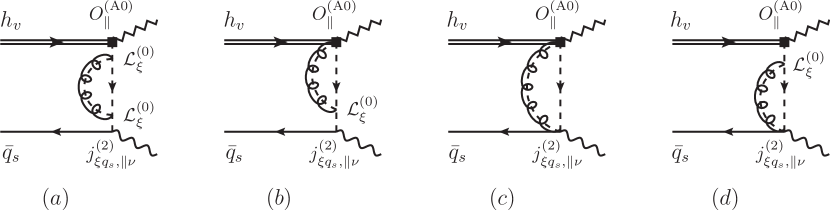
Figure 1: Diagrammatical representation of the vacuum-to-$B$-meson correlation function $\Pi_{\nu,\|}^{A}(p,q)$ defined with the ${\rm A0}$-type SCET operator $O_{\|}^{\rm{(A0)}}=\left(\bar{\xi}\,W_{c}\right)\,\gamma_{5}\,h_{v}$ and the power suppressed interpolating current $j_{\xi q_{s},\parallel\,\nu}^{(2)}$ at one loop.

We proceed to determine the NLO contribution to the jet function $J_{\|,\pm}^{A}$ by expanding the matching relation (23) up to the ${\cal O}(\alpha_{s})$ accuracy. To this end, we will need to evaluate the one-loop ${\rm SCET}_{\rm I}$ diagrams presented in figure 1 with the subleading power SCET Feynman rules collected in [53]. The self-energy correction to the hard-collinear quark propagator displayed in the diagram (a) of figure 1 can be readily written as [54]

$$F_{\|,\,{\rm NLO}}^{A,(a)}=-{\alpha_{s}\,C_{F}\over 4\,\pi}\,\left[{1\over\epsilon}+\ln{\mu^{2}\over n\cdot p\,(\omega-\bar{n}\cdot p)-i0}+1\right]\,F_{\|,\,{\rm LO}}^{A}\,.$$ (27)

Obviously, the NLO correction from the hard-collinear Wilson lines presented in the diagram (c) of figure 1 yields vanishing contribution due to $n^{2}=0$. One can further verify that the hard-collinear corrections displayed in the diagrams (b) and (d) of figure 1 give rise to the identical results

$$F_{\|,\,{\rm NLO}}^{A,(b)} = F_{\|,\,{\rm NLO}}^{A,(d)}=-{2\,g_{s}^{2}\,C_{F}\over\bar{n}\cdot p-\omega}\,\,\bar{q}_{s}(k)\,{\not\!n\over 2}\,\gamma_{5}\,h_{v}\,$$ (28)

$$\times\,\int{d^{D}l\over(2\pi)^{D}}\,{n\cdot(p+l)\over[n\cdot(p+l)\,\bar{n}\cdot(p-k+l)+l_{\perp}^{2}+i0][n\cdot l+i0][l^{2}+i0]}\,,$$

which can be evaluated straightforwardly with dimensional regularization scheme

$$F_{\|,\,{\rm NLO}}^{A,(b)} = F_{\|,\,{\rm NLO}}^{A,(d)}={\alpha_{s}\,C_{F}\over 2\,\pi}\,\,\bigg{\{}{1\over\epsilon^{2}}+{1\over\epsilon}\,\left[\ln{\mu^{2}\over n\cdot p\,(\omega-\bar{n}\cdot p)}+1\right]+{1\over 2}\,\ln^{2}{\mu^{2}\over n\cdot p\,(\omega-\bar{n}\cdot p)}$$ (29)

$$+\,\ln{\mu^{2}\over n\cdot p\,(\omega-\bar{n}\cdot p)}-{\pi^{2}\over 12}+2\bigg{\}}\,\,F_{\|,\,{\rm LO}}^{A}\,.$$

Adding up different pieces together and applying the matching condition (23) leads to the hard-collinear functions at the one-loop accuracy

$$J_{\|,\,-}^{A,\,(1)} = J_{\|,\,-}^{A,\,(0)}\,\bigg{\{}1+{\alpha_{s}\,C_{F}\over 4\,\pi}\,\bigg{[}{4\over\epsilon^{2}}+{1\over\epsilon}\,\left(4\,\ln{\mu^{2}\over n\cdot p\,(\omega-\bar{n}\cdot p)}+3\right)+2\,\ln^{2}{\mu^{2}\over n\cdot p\,(\omega-\bar{n}\cdot p)}$$

$$+\,3\,\ln{\mu^{2}\over n\cdot p\,(\omega-\bar{n}\cdot p)}-{\pi^{2}\over 3}+7\bigg{]}\bigg{\}}\,,$$

$$J_{\|,\,+}^{A,\,(1)} = 0\,,$$ (30)

which are in precise agreement with the results presented in [26].

3.1.2 SCET factorization for $\Pi_{\nu,\|}^{B}(p,q)$

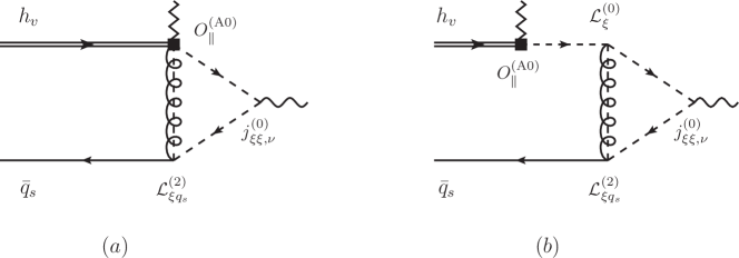
Figure 2: Diagrammatical representation of the vacuum-to-$B$-meson correlation function $\Pi_{\nu,\|}^{B}(p,q)$ defined with the ${\rm A0}$-type SCET operator $O_{\|}^{\rm{(A0)}}=\left(\bar{\xi}\,W_{c}\right)\,\gamma_{5}\,h_{v}$, the leading power interpolating current $j_{\xi\xi,\nu}^{(0)}$ and the subleading power SCET Lagrangian ${\cal L}_{\xi q_{s}}^{(2)}$.

Along the same vein, the jet function $J_{\|,\,\pm}^{B}$ can be determined by performing the perturbative factorization for the partonic matrix element

$$F_{\|}^{B}=\int d^{4}x\,e^{ip\cdot x}\,\int d^{4}y\,\left\langle 0\left|{\rm T}\left\{\bar{\xi}(x)\,{\not\!n\over 2}\,\xi(x),\,\,i\,{\cal L}_{\xi q_{s}}^{(2)}(y),\,\,\left(\bar{\xi}\,W_{c}\right)(0)\,\gamma_{5}\,h_{v}(0)\,\right\}\right|\bar{q}_{s}(k)\,h_{v}\right\rangle,\hskip 14.22636pt$$ (31)

taking advantage of the matching relation in analogy to (23)

$$F_{\|}^{B}=(-i)\,\sum_{m=\pm}\,J_{\|,\,m}^{B}\left({\mu^{2}\over n\cdot p\,\omega^{\prime}},{\omega^{\prime}\over\bar{n}\cdot p}\right)\,\ast\langle O_{\|,\,m}\,(\omega,\omega^{\prime})\rangle\,.$$ (32)

Evaluating the diagram (a) in figure 2 with the SCET Feynman rules leads to

$$F_{\|,\rm{LO}}^{B,(a)} = -2\,g_{s}^{2}\,C_{F}\,\bar{q}_{s}(k)\,{\not\!n\over 2}\,\gamma_{5}\,h_{v}$$ (33)

$$\times\,\int{d^{D}l\over(2\pi)^{D}}\,{n\cdot(p-l)\over[n\cdot l\,\bar{n}\cdot(l+k)+l_{\perp}^{2}+i0][n\cdot(p-l)\,\bar{n}\cdot(p-l-k)+l_{\perp}^{2}+i0][l^{2}+i0]}\,$$

$$= {\alpha_{s}\,C_{F}\over 2\,\pi}\,{\bar{n}\cdot p-\omega\over\omega}\,\left[{1\over\epsilon}+\ln{\mu^{2}\over n\cdot p\,(\omega-\bar{n}\cdot p)}+{1\over 2}\,\left({\bar{n}\cdot p-\omega\over\bar{n}\cdot p}\right)+1\right]$$

$$\times\,\ln\left({\bar{n}\cdot p-\omega\over\bar{n}\cdot p}\right)\,F_{\|,\,{\rm LO}}^{A}.$$

We can proceed to write down the QCD amplitude for the diagram (b) in figure 2

$$F_{\|,\rm{LO}}^{B,(b)} = g_{s}^{2}\,C_{F}\,\int{d^{D}l\over(2\pi)^{D}}\,\int{d^{D}L\over(2\pi)^{D}}\frac{n\cdot L\,\,n\cdot(p+L)\,\,n\cdot(p+L+l)}{[L^{2}+i0][(p+L)^{2}+i0][(p+L+l)^{2}+i0][l^{2}+i0]}$$ (34)

$$\bar{q}_{s}(k)\,\bigg{\{}(2\,\pi)^{4}\,\delta^{4}(l+L+k)\,\left[\bar{n}^{\alpha}+\gamma_{\perp}^{\alpha}\,{\not\!L_{\perp}\over n\cdot L}+{n^{\alpha}\over n\cdot l}\,{L^{2}\over n\cdot L}\right]\,{\not\!n\over 2}$$

$$+\,k_{\perp\,\beta}\,\partial_{\perp}^{\beta}\,\left[(2\,\pi)^{4}\,\delta^{4}(l+L+k)\right]\,\left[\gamma_{\perp}^{\alpha}-{\not\!L_{\perp}\over n\cdot L}\,n^{\alpha}\right]\,\bigg{\}}$$

$$\left[\bar{n}_{\alpha}+{\gamma_{\alpha\,\perp}\,(\not\!L_{\perp}+\not l_{\perp})\over n\cdot(p+L+l)}+{\not\!L_{\perp}\,\gamma_{\alpha\perp}\over n\cdot(p+L)}-{L_{\perp}^{2}+\not\!L_{\perp}\,\not l_{\perp}\over n\cdot(p+L)\,n\cdot(p+L+l)}\,n_{\alpha}\right]\,{\not\!\bar{n}\over 2}\,\gamma_{5}\,h_{v}\,,\hskip 14.22636pt$$

which can be further evaluated with two distinct approaches by identifying the transverse derivative $\partial_{\perp}^{\beta}$ acting on the Dirac $\delta$-function as $\partial/\partial k_{\perp\beta}$ and $\partial/\partial L_{\perp\beta}$, respectively. We have verified explicitly that both the two calculational methods lead to the identical results

$$F_{\|,\rm{LO}}^{B,(b)} = {\alpha_{s}\,C_{F}\over 4\,\pi}\,\bigg{\{}-{2\over\epsilon^{2}}+{1\over\epsilon}\,\left[-2\,\ln\left({\mu^{2}\over n\cdot p\,(\omega-\bar{n}\cdot p)}\right)+\,2\,\,{\ln(1+\eta)\over\eta}-3\right]$$ (35)

$$-\ln^{2}\left({\mu^{2}\over n\cdot p\,(\omega-\bar{n}\cdot p)}\right)+\ln\left({\mu^{2}\over n\cdot p\,(\omega-\bar{n}\cdot p)}\right)\,\left[2\,\,{\ln(1+\eta)\over\eta}-3\right]$$

$$+\,{1\over\eta}\,\ln^{2}(1+\eta)+\left({4\over\eta}+1\right)\,\ln(1+\eta)+{\pi^{2}\over 6}-8\bigg{\}}\,\,F_{\|,\,{\rm LO}}^{A}\,,$$

where we have defined $\eta=-\omega/\bar{n}\cdot p$. Applying the matching condition for the matrix element $F_{\|}^{B}$ presented in (32) we can readily derive the hard-collinear function $J_{\|,\,\pm}^{B}$ at tree level

$$J_{\|,\,-}^{B} = {\alpha_{s}\,C_{F}\over 4\,\pi}\,J_{\|,\,-}^{A,\,(0)}\,\bigg{\{}-{2\over\epsilon^{2}}+{1\over\epsilon}\,\left[-2\,\ln\left({\mu^{2}\over n\cdot p\,(\omega-\bar{n}\cdot p)}\right)-2\,\ln(1+\eta)-3\right]$$

$$-\,\ln^{2}\left({\mu^{2}\over n\cdot p\,(\omega-\bar{n}\cdot p)}\right)+\ln\left({\mu^{2}\over n\cdot p\,(\omega-\bar{n}\cdot p)}\right)\,\left[-2\,\ln(1+\eta)-3\right]-\ln^{2}(1+\eta)$$

$$+\,\left({2\over\eta}-1\right)\,\ln(1+\eta)+{\pi^{2}\over 6}-8\bigg{\}}\,,$$

$$J_{\|,\,+}^{B} = 0\,,$$ (36)

which are again in complete agreement with the previous calculations displayed in [26].

3.1.3 SCET factorization for $\Pi_{\nu,\|}^{C}(p,q)$

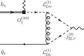
Figure 3: Diagrammatical representation of the vacuum-to-$B$-meson correlation function $\Pi_{\nu,\|}^{B}(p,q)$ defined with the ${\rm A0}$-type SCET operator $O_{\|}^{\rm{(A0)}}=\left(\bar{\xi}\,W_{c}\right)\,\gamma_{5}\,h_{v}$, the leading power interpolating current $j_{\xi\xi,\nu}^{(0)}$ and the subleading power SCET Lagrangians ${\cal L}_{\xi q_{s}}^{(1)}$ and ${\cal L}_{\xi m}^{(1)}$.

We are now in a position to compute the jet function $J_{\|,\,\pm}^{C}$ entering the SCET factorization formula (17) by inspecting the QCD matrix element

$$F_{\|}^{C} = \int d^{4}x\,e^{ip\cdot x}\,\int d^{4}y\,\int d^{4}z\,$$ (37)

$$\left\langle 0\left|{\rm T}\left\{\bar{\xi}(x)\,{\not\!n\over 2}\,\xi(x),\,\,i\,{\cal L}_{\xi q_{s}}^{(1)}(y),\,\,i\,{\cal L}_{\xi m}^{(1)}(z),\,\,\left(\bar{\xi}\,W_{c}\right)(0)\,\gamma_{5}\,h_{v}(0)\,\right\}\right|\bar{q}_{s}(k)\,h_{v}\right\rangle\,,$$

which can be further matched onto the light-ray HQET operators defining the $B$-meson LCDA

$$F_{\|}^{C}=(-i)\,\sum_{m=\pm}\,J_{\|,\,m}^{C}\left({\mu^{2}\over n\cdot p\,\omega^{\prime}},{\omega^{\prime}\over\bar{n}\cdot p}\right)\,\ast\langle O_{\|,\,m}\,(\omega,\omega^{\prime})\rangle\,.$$ (38)

The LO amplitude of $F_{\|}^{C}$ can be obtained by computing the diagram in figure 3

$$F_{\|,\rm{LO}}^{C} = -{m\over n\cdot p}\,{g_{s}^{2}\,C_{F}\over\bar{n}\cdot p-\omega}\,\,\bar{q}_{s}(k)\,{\not\!\bar{n}\over 2}\,\gamma_{5}\,h_{v}\,$$ (39)

$$\times\,\int{d^{D}l\over(2\pi)^{D}}\,{(D-2)\,(n\cdot l)^{2}\over[n\cdot l\,\bar{n}\cdot(l+k)+l_{\perp}^{2}+i0][n\cdot(p-l)\,\bar{n}\cdot(p-l-k)+l_{\perp}^{2}+i0][l^{2}+i0]}\,$$

$$= {m\over\omega}\,{\alpha_{s}\,C_{F}\over 4\,\pi}\,{i\over\bar{n}\cdot p-\omega+i0}\,\ln\left({\bar{n}\cdot p-\omega\over\bar{n}\cdot p}\right)\,\bar{q}_{s}(k)\,{\not\!\bar{n}\over 2}\,\gamma_{5}\,h_{v},$$

where $m$ indicates the mass of the collinear quark produced from the weak decay of the heavy quark. It is evident that the light-quark mass effect defined by $F_{\|}^{C}$ is not suppressed by any powers of $\Lambda/m_{b}$ in the heavy quark expansion compared with the SCET matrix elements $F_{\|}^{A}$ and $F_{\|}^{B}$ . The resulting jet functions at tree level $J_{\|,\,\pm}^{C}$ are given by

$$J_{\|,\,+}^{C} = -{m\over\omega}\,{1\over\bar{n}\cdot p-\omega+i0}\,{\alpha_{s}\,C_{F}\over 4\,\pi}\,\ln\left({\bar{n}\cdot p-\omega\over\bar{n}\cdot p}\right)\,,$$

$$J_{\|,\,-}^{C} = 0\,,$$ (40)

which are consistent with the results derived from the diagrammatic factorization approach for the corresponding vacuum-to-$B$-meson correlation function in QCD [22].

Plugging the obtained jet functions (30), (36) and (40) into the factorization formula (17) and employing the decomposition of $\Pi_{\nu,\|}$ defined in (15) yields

$$\Pi_{\nu,\|}(p,q) = {\tilde{f}_{B}(\mu)\,m_{B}\over 2}\,\,\int_{0}^{+\infty}\,{d\omega\over\bar{n}\cdot p-\omega+i0}\,\bigg{\{}\left[1+{\alpha_{s}\,C_{F}\over 4\,\pi}\,\hat{J}_{\|,-}^{(\rm A0)}\left({\mu^{2}\over n\cdot p\,\omega},{\omega\over\bar{n}\cdot p}\right)\right]\,\phi_{B}^{-}(\omega,\mu)\,\,$$ (41)

$$+\left[\,{\alpha_{s}\,C_{F}\over 4\,\pi}\,\hat{J}_{\|,+}^{(m)}\left({\mu^{2}\over n\cdot p\,\omega},{\omega\over\bar{n}\cdot p}\right)\right]\,\phi_{B}^{+}(\omega,\mu)\bigg{\}}\,\,\bar{n}_{\nu}\,,$$

where the normalized one-loop jet functions $\hat{J}_{\|,-}^{(\rm A0)}$ and $\hat{J}_{\|,+}^{(m)}$ read

$$\hat{J}_{\|,-}^{(\rm A0)} = \ln^{2}\left({\mu^{2}\over n\cdot p\,(\omega-\bar{n}\cdot p)}\right)-2\,\ln\left({\mu^{2}\over n\cdot p\,(\omega-\bar{n}\cdot p)}\right)\,\ln(1+\eta)-\ln^{2}(1+\eta)$$

$$+\left({2\over\eta}-1\right)\,\ln(1+\eta)-{\pi^{2}\over 6}-1\,,$$

$$\hat{J}_{\|,+}^{(m)} = -{m\over\omega}\,\ln\left({\bar{n}\cdot p-\omega\over\bar{n}\cdot p}\right)\,.$$ (42)

To facilitate the construction of the SCET sum rules for the effective form factor $\xi_{\|}(n\cdot p)$, we need to work out the dispersion representation of the factorization formula (41) by computing the spectral functions of the various convolution integrations over the variable $\omega$

$$\Pi_{\nu,\|}(p,q) = -{\tilde{f}_{B}(\mu)\,m_{B}\over 2}\,\,\int_{0}^{+\infty}\,{d\omega^{\prime}\over\omega^{\prime}-\bar{n}\cdot p-i0}\,\left[\phi_{B,\rm{eff}}^{-}(\omega^{\prime},\mu)+\phi_{B,m}^{+}(\omega^{\prime},\mu)\right]\,\bar{n}_{\nu}\,,$$ (43)

where the effective $B$-meson “distribution amplitudes” are introduced to describe both the hard-collinear and soft fluctuations [20, 22]

$$\phi_{B,\rm{eff}}^{-}(\omega^{\prime},\mu) = \phi_{B}^{-}(\omega^{\prime},\mu)+{\alpha_{s}\,C_{F}\over 4\,\pi}\,\bigg{\{}\int_{0}^{\omega^{\prime}}d\omega\,\left[{2\over\omega-\omega^{\prime}}\,\left(\ln{\mu^{2}\over n\cdot p\,\omega^{\prime}}-2\,\ln{\omega^{\prime}-\omega\over\omega^{\prime}}\right)\right]_{\oplus}\,\phi_{B}^{-}(\omega,\mu)$$

$$-\int_{\omega^{\prime}}^{\infty}\,d\omega\,\left[\ln^{2}{\mu^{2}\over n\cdot p\,\omega^{\prime}}-\left(2\,\ln{\mu^{2}\over n\cdot p\,\omega^{\prime}}+3\right)\,\ln{\omega-\omega^{\prime}\over\omega^{\prime}}+2\,\ln{\omega\over\omega^{\prime}}+{\pi^{2}\over 6}-1\right]\,$$

$$\times\,{d\phi_{B}^{-}(\omega,\mu)\over d\omega}\bigg{\}}\,,$$

$$\phi_{B,m}^{+}(\omega^{\prime},\mu) = {\alpha_{s}\,C_{F}\over 4\,\pi}\,m\,\int_{\omega^{\prime}}^{\infty}d\omega\,\ln{\omega-\omega^{\prime}\over\omega^{\prime}}\,\,{d\over d\omega}\,{\phi_{B}^{+}(\omega,\mu)\over\omega}\,.$$ (44)

The plus function appearing in (44) is defined in the standard way [47]

$$\int_{0}^{\omega^{\prime}}\,\,d\omega\,[f(\omega,\omega^{\prime})]_{\oplus}\,\,g(\omega)=\int_{0}^{\omega^{\prime}}\,\,d\omega\,f(\omega,\omega^{\prime})\,\,[g(\omega)-g(\omega^{\prime})]\,.$$ (45)

Matching the spectral representation of the factorization formula (43) for the vacuum-to-$B$-meson correlation function $\Pi_{\nu,\|}$ with the corresponding hadronic dispersion relation

$$\Pi_{\nu,\|}(p,q)$$

$$=\left[-{f_{V,\|}\,m_{V}\over m_{V}^{2}/n\cdot p-\bar{n}\cdot p-i0}\,\left({n\cdot p\over 2\,m_{V}}\right)^{2}\,\xi_{\|}(n\cdot p)+\int_{\omega_{s}}^{+\infty}\,{d\omega^{\prime}\over\omega^{\prime}-\bar{n}\cdot p-i0}\,\,\rho^{h}_{\|}(\omega^{\prime},n\cdot p)\right]\,\bar{n}_{\nu}\,,\hskip 22.76228pt$$ (46)

we can readily derive the NLO sum rules for the SCET form factor $\xi_{\|}(n\cdot p)$

$$\xi_{\|,\,\rm{NLO}}(n\cdot p)$$

$$=2\,{\tilde{f}_{B}(\mu)\over f_{V,\|}}\,{m_{B}\,m_{V}\over(n\cdot p)^{2}}\,\int_{0}^{\omega_{s}}\,d\omega^{\prime}\,{\rm exp}\left[-{n\cdot p\,\omega^{\prime}-m_{V}^{2}\over n\cdot p\,\omega_{M}}\right]\left[\phi_{B,\rm{eff}}^{-}(\omega^{\prime},\mu)+\phi_{B,m}^{+}(\omega^{\prime},\mu)\right]\,.\hskip 14.22636pt$$ (47)

The scale-independent longitudinal decay constant of the vector meson is defined as follows

$$c_{V}\,\langle V(p,\epsilon^{\ast})|j_{\nu}|0\rangle=-i\,f_{V,\|}\,\,m_{V}\,\,\epsilon^{\ast}_{\nu}(p)\,.$$ (48)

The HQET $B$-meson decay constant $\tilde{f}_{B}(\mu)$ will be expressed in terms of the QCD decay constant $f_{B}$ at one loop [55]

$$\tilde{f}_{B}(\mu)=\left[1-{\alpha_{s}\,C_{F}\over 4\,\pi}\,\left(3\ln{\mu\over m_{b}}+2\right)\right]^{-1}\,f_{B}=K^{-1}(m_{b},\mu)\,f_{B}\,.$$ (49)

Taking the factorization scale $\mu$ as a hard-collinear scale $\mu_{hc}\sim\sqrt{\Lambda\,m_{b}}$ will introduce the enhanced logarithms of $m_{b}/\mu$ in the perturbative matching coefficient $K(m_{b},\mu)$, whose resummation at the NLL accuracy can be achieved with the standard RG approach. Solving the two-loop RG evolution equation for the HQET decay constant $\tilde{f}_{B}(\mu)$ [56, 57] leads to

$$\tilde{f}_{B}(\mu)=U_{2}(\mu_{h2},\mu)\,\tilde{f}_{B}(\mu_{h2})\,,$$ (50)

where the explicit expression of the evolution function $U_{2}(\mu_{h2},\mu)$ has been derived in [55, 58]. Since the soft scale $\mu_{0}$ entering the initial condition of the $B$-meson distribution amplitudes $\phi_{B}^{\pm}(\omega,\mu_{0})$ is numerically comparable to the hard-collinear scale $\mu_{hc}\simeq 1.5\,{\rm GeV}$, we not perform the NLL resummation of the parametrically large logarithms of $\mu/\mu_{0}$ by applying the Lange-Neubert evolution equation at two loops [59]. It is then straightforward to write down the resummation improved SCET sum rules for $\xi_{\|}(n\cdot p)$

$$\xi_{\|,\,\rm{NLL}}(n\cdot p) = 2\,{U_{2}(\mu_{h2},\mu)\,\tilde{f}_{B}(\mu_{h2})\over f_{V,\|}}\,{m_{B}\,m_{V}\over(n\cdot p)^{2}}\,$$ (51)

$$\times\,\int_{0}^{\omega_{s}}\,d\omega^{\prime}\,{\rm exp}\left[-{n\cdot p\,\omega^{\prime}-m_{V}^{2}\over n\cdot p\,\omega_{M}}\right]\,\left[\phi_{B,\rm{eff}}^{-}(\omega^{\prime},\mu)+\phi_{B,m}^{+}(\omega^{\prime},\mu)\right]\,.$$

3.2 The $B$-meson LCSR for $\Xi_{\parallel}(\tau,n\cdot p)$

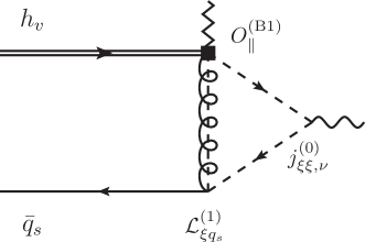
Figure 4: Diagrammatical representation of the vacuum-to-$B$-meson correlation function $\widetilde{\Pi}_{\nu,\|}(p,q,\tau)$ defined with the ${\rm B1}$-type SCET operator $O_{\|}^{\rm{(B1)}}=(\bar{\xi}\,W_{c})(0)\,\gamma_{5}\,\,(W_{c}^{\dagger}\,\,i{\not\!\!D_{c,\,\perp}}\,\,W_{c})(r\,n)\,\,h_{v}(0)$, the leading power interpolating current $j_{\xi\xi,\nu}^{(0)}$ for the longitudinal polarized vector meson and the subleading power SCET Lagrangian ${\cal L}_{\xi q_{s}}^{(1)}$.

We aim at constructing the SCET sum rules for the $\rm{B1}$-type non-local form factor $\Xi_{\parallel}(\tau,n\cdot p)$ from the following correlation function

$$\widetilde{\Pi}_{\nu,\|}(p,q,\tau) = {n\cdot p\over 2\,\pi}\,\int d^{4}x\,e^{ip\cdot x}\,\int dr\,e^{-in\cdot p\,\tau\,r}\,$$ (52)

$$\langle 0|{\rm T}\left\{j_{\nu}(x),\,\,\left(\bar{\xi}\,W_{c}\right)(0)\,\gamma_{5}\,\,(W_{c}^{\dagger}\,\,i\not\!\!D_{c,\,\perp}\,W_{c})(r\,n)\,\,h_{v}(0)\,\right\}|\bar{B}_{v}\rangle\,,$$

the leading power contribution of which can be readily identified as

$$\widetilde{\Pi}_{\nu,\|}(p,q,\tau) = {n\cdot p\over 2\,\pi}\,\int d^{4}x\,e^{ip\cdot x}\,\int d^{4}y\,\int dr\,e^{-in\cdot p\,\tau\,r}\,$$ (53)

$$\langle 0|{\rm T}\left\{j_{\xi\xi,\nu}^{(0)}(x),\,\,i\,{\cal L}_{\xi q_{s}}^{(1)}(y),\,\,\left(\bar{\xi}\,W_{c}\right)(0)\,\gamma_{5}\,\,(W_{c}^{\dagger}\,\,i\not\!D_{c,\,\perp}\,W_{c})(r\,n)\,\,h_{v}(0)\,\right\}|\bar{B}_{v}\rangle\,.\hskip 14.22636pt$$

The soft-collinear factorization formula for the vacuum-to-$B$-meson correlation function $\widetilde{\Pi}_{\nu,\|}$ can be obtained by integrating out the hard-collinear dynamics

$$\widetilde{\Pi}_{\nu,\|}(p,q,\tau)={\tilde{f}_{B}(\mu)\,m_{B}\over 2}\,\sum_{m=\pm}\,\int_{0}^{+\infty}\,d\omega\,\tilde{J}_{\|,m}\left({\mu^{2}\over n\cdot p\,\omega},{\omega\over\bar{n}\cdot p},\tau\right)\,\phi_{B}^{m}(\omega,\mu)\,\,\bar{n}_{\nu}.\,\,\,$$ (54)

The short-distance matching coefficient functions $\tilde{J}_{\|,m}$ can be determined by investigating the SCET matrix element

$$\tilde{F}_{\|}(p,q,\tau) = {n\cdot p\over 2\,\pi}\,\int d^{4}x\,e^{ip\cdot x}\,\int d^{4}y\,\int dr\,e^{-in\cdot p\,\tau\,r}\,\bigg{\langle}0\bigg{|}{\rm T}\bigg{\{}\bar{\xi}(x)\,{\not\!n\over 2}\,\xi(x),\,\,i\,{\cal L}_{\xi q_{s}}^{(1)}(y),\,\,$$ (55)

$$\left(\bar{\xi}\,W_{c}\right)(0)\,\gamma_{5}\,\,(W_{c}^{\dagger}\,\,i\not\!\!D_{c\,\perp}\,W_{c})(r\,n)\,\,h_{v}(0)\,\bigg{\}}\bigg{|}\bar{q}_{s}(k)\,h_{v}\bigg{\rangle}\,.$$

Evaluating the tree-level diagram displayed in figure 4 with the SCET Feynman rules yields

$$\tilde{F}_{\|}(p,q,\tau) = g_{s}^{2}\,C_{F}\,\,\bar{q}_{s}(k)\,{\not\!\bar{n}\over 2}\,\gamma_{5}\,h_{v}$$ (56)

$$\int{d^{D}l\over(2\pi)^{D}}\,{(D-2)\,n\cdot l\,n\cdot(p-l)\,\delta(\tau-n\cdot l/n\cdot p)\over[n\cdot l\,\bar{n}\cdot(l+k)+l_{\perp}^{2}+i0][n\cdot(p-l)\,\bar{n}\cdot(p-l-k)+l_{\perp}^{2}+i0][l^{2}+i0]}\,,\hskip 22.76228pt$$

which can be further computed with the contour integration method

$$\tilde{F}_{\|}(p,q,\tau) = \left(-i\right)\,{\alpha_{s}\,C_{F}\over 2\,\pi}\,{n\cdot p\over\omega}\,\ln(1+\eta)\,\left[(1-\tau)\,\theta(\tau)\,\theta(1-\tau)\right]\,\,\,\bar{q}_{s}(k)\,{\not\!\bar{n}\over 2}\,\gamma_{5}\,h_{v}\,.$$ (57)

Applying the matching relation for the SCET matrix element $\tilde{F}_{\|}(p,q,\tau)$

$$\tilde{F}_{\|}(p,q,\tau)=(-i)\,\sum_{m=\pm}\,\tilde{J}_{\|,\,m}\left({\mu^{2}\over n\cdot p\,\omega^{\prime}},{\omega^{\prime}\over\bar{n}\cdot p},\tau\right)\,\ast\langle O_{\|,\,m}\,(\omega,\omega^{\prime})\rangle\,,$$ (58)

we obtain the jet functions entering the factorization formula (54) at tree level

$$\tilde{J}_{\|,\,+}={\alpha_{s}\,C_{F}\over 2\,\pi}\,{n\cdot p\over\omega}\,\ln(1+\eta)\,\left[(1-\tau)\,\theta(\tau)\,\theta(1-\tau)\right]\,,\qquad\tilde{J}_{\|,\,-}=0.$$ (59)

Matching the spectral representation of the SCET factorization formula (54) for the correlation function $\widetilde{\Pi}_{\nu,\|}$

$$\widetilde{\Pi}_{\nu,\|}(p,q,\tau) = {\alpha_{s}\,C_{F}\over 4\,\pi}\,\tilde{f}_{B}(\mu)\,m_{B}\,\left[(1-\tau)\,\theta(\tau)\,\theta(1-\tau)\right]\,$$ (60)

$$\times\,\int_{0}^{\infty}{d\omega^{\prime}\over\omega^{\prime}-\bar{n}\cdot p-i0}\,\left[\int_{\omega^{\prime}}^{\infty}d\omega\,{n\cdot p\over\omega}\,\phi_{B}^{+}(\omega,\mu)\right]\,\bar{n}_{\nu}\,$$

with the corresponding hadronic representation

$$\widetilde{\Pi}_{\nu,\|}(p,q,\tau) = \bigg{[}-{f_{V,\|}\,\,m_{V}\over m_{V}^{2}/n\cdot p-\bar{n}\cdot p-i0}\,\left({n\cdot p\over 2\,m_{V}}\right)^{2}\,m_{b}\,\,\Xi_{\|}(\tau,n\cdot p)$$ (61)

$$+\int_{\omega_{s}}^{+\infty}\,{d\omega^{\prime}\over\omega^{\prime}-\bar{n}\cdot p-i0}\,\,\tilde{\rho}^{h}_{\|}(\omega^{\prime},n\cdot p,\tau)\bigg{]}\,\bar{n}_{\nu}\,,$$

and employing the parton-hadron duality approximation with the aid of the Borel transformation, we can derive the SCET sum rules for the non-local form factor $\Xi_{\|}(\tau,n\cdot p)$

$$\Xi_{\|}(\tau,n\cdot p) = -{\alpha_{s}\,C_{F}\over\pi}\,{U_{2}(\mu_{h2},\mu)\,\,\tilde{f}_{B}(\mu_{h2})\over f_{V,\|}}\,{m_{B}\,m_{V}\over\,n\cdot p\,m_{b}}\,\,\left[(1-\tau)\,\theta(\tau)\,\theta(1-\tau)\right]\,$$ (62)

$$\times\,\int_{0}^{\omega_{s}}\,d\omega^{\prime}\,{\rm exp}\left[-{n\cdot p\,\omega^{\prime}-m_{V}^{2}\over n\cdot p\,\omega_{M}}\right]\int_{\omega^{\prime}}^{\infty}\,d\omega\,{\phi_{B}^{+}(\omega,\mu)\over\omega}\,+{\cal O}(\alpha_{s}^{2})\,,$$

where the summation of the enhanced logarithms of $m_{b}/\mu$ entering the hard matching coefficient $K^{-1}(m_{b},\mu)$ has been included at the LL accuracy.

It will be interesting to compare the obtained sum rules for $\Xi_{\|}(\tau,n\cdot p)$ presented in (62) with the direct QCD calculation in the SCET framework. Integrating the hard-collinear fluctuations, the ${\rm B}$-type ${\rm SCET}_{\rm I}$ form factor $\Xi_{\|}(\tau,n\cdot p)$ can be further factorized as the convolution of the short-distance coefficient function and distributions amplitudes of the $B$-meson and the vector meson in ${\rm SCET}_{\rm II}$

$$\Xi_{\|}^{\rm{SCET}}(\tau,n\cdot p) = {2\,m_{V}\over n\cdot p}\,{m_{B}\over 4\,m_{b}}\,\left[U_{2}(\mu_{h2},\mu)\,\,\tilde{f}_{B}(\mu_{h2})\right]\,f_{V,\|}\,$$ (63)

$$\times\,\int_{0}^{\infty}\,d\omega\,\int_{0}^{1}dv\,\phi_{B}^{+}(\omega,\mu)\,\phi_{V,\|}(v,\mu)\,J_{V,\|}^{\rm{SCET}}(\tau,v,\omega)\,,$$

where the jet function $J_{V,\|}^{\rm{SCET}}$ has been determined at NLO in $\alpha_{s}$ [42] by implementing the ultraviolet renormalization and the infrared subtraction with the dimensional regularization scheme and the evanescent operator approach. Substituting the tree-level expression of $J_{V,\|}^{\rm{SCET}}$ into the SCET factorization formula (63) and employing the asymptotic form of the vector-meson distribution amplitude $\phi_{V,\|}(v,\mu)=6\,v\,(1-v)$ leads to

$$\Xi_{\|,\,\rm{LO}}^{\rm{SCET}}(\tau,n\cdot p) = -{3\,g_{s}^{2}\,C_{F}\over N_{c}}\,{m_{B}\,m_{V}\over(n\cdot p)^{2}\,m_{b}}\,\left[U_{2}(\mu_{h2},\mu)\,\,\tilde{f}_{B}(\mu_{h2})\right]\,f_{V,\|}\,\,\left[(1-\tau)\,\theta(\tau)\,\theta(1-\tau)\right]\,$$ (64)

$$\times\,\int_{0}^{\infty}\,{d\omega\over\omega}\,\phi_{B}^{+}(\omega,\mu)\,.$$

Based upon the power counting scheme for the sum rule parameters

$$\omega_{s}\sim\omega_{M}\sim{\cal O}\left({\Lambda^{2}/m_{b}}\right)\,,$$ (65)

the resummation improved SCET sum rules (62) for $\Xi_{\|}(\tau,n\cdot p)$ can be further reduced to

$$\Xi_{\|}(\tau,n\cdot p) = -{\alpha_{s}\,C_{F}\over\pi}\,{U_{2}(\mu_{h2},\mu)\,\,\tilde{f}_{B}(\mu_{h2})\over f_{V,\|}}\,{m_{B}\,m_{V}\over\,n\cdot p\,m_{b}}\,\,\left[(1-\tau)\,\theta(\tau)\,\theta(1-\tau)\right]\,$$ (66)

$$\times\,\int_{0}^{\infty}\,{d\omega\over\omega}\,\phi_{B}^{+}(\omega,\mu)\,\,\left\{\omega_{M}\,\left(1-e^{-\omega_{s}/\omega_{M}}\right)\,{\rm exp}\left[{m_{V}^{2}\over n\cdot p\,\omega_{M}}\right]\right\}\,,$$

which can be readily demonstrated to be identical to the tree-level SCET factorization formula (64) by employing the QCD sum rules for the vector-meson decay constant at leading power approximation [60]

$$f_{V,\|}^{2}={N_{c}\over 12\,\pi^{2}}\,n\cdot p\,\omega_{M}\,\left\{\left(1-e^{-\omega_{s}/\omega_{M}}\right)\,{\rm exp}\left[{m_{V}^{2}\over n\cdot p\,\omega_{M}}\right]\right\}+{\cal O}(\alpha_{s})\,.$$ (67)

However, we mention in passing that the advantage of the SCET factorization over the LCSR approach presented here lies in the fact that it is free of the systematic uncertainty induced by the parton-hadron duality approximation of the light-meson channel and the perturbative correction to the hard-collinear function $\Xi_{\|}(\tau,n\cdot p)$ at ${\cal O}(\alpha_{s}^{\ell})$ can be determined by computing the ${\rm SCET}_{\rm I}$ Feynman diagrams at $(\ell-1)$ loops instead of evaluating the effective diagrams for the vacuum-to-$B$-meson correlation function $\widetilde{\Pi}_{\nu,\|}(p,q,\tau)$ at $\ell$ loops.

3.3 The $B$-meson LCSR for $\xi_{\perp}(n\cdot p)$

We proceed to construct the SCET sum rules for the $\rm{A0}$-type form factor $\xi_{\perp}(n\cdot p)$ by investigating the following vacuum-to-$B$-meson correlation function

$$\Pi_{\mu\nu\rho,\perp}(p,q)=\int d^{4}x\,e^{ip\cdot x}\,\langle 0|{\rm T}\left\{j_{\nu\rho}(x),\,\,\left(\bar{\xi}\,W_{c}\right)(0)\,\gamma_{5}\,\gamma_{\mu\,\perp}\,h_{v}(0)\,\right\}|\bar{B}_{v}\rangle\,,$$ (68)

where the interpolating current for the transversely polarized vector meson is given by

$$j_{\nu\rho}(x)=\bar{q}^{\prime}(x)\,\gamma_{\nu}\,\gamma_{\rho\,\perp}\,q(x)\,.$$ (69)

Matching the QCD interpolating current $j_{\nu\rho}$ onto ${\rm SCET}_{\rm I}$ yields

$$j_{\nu\rho}(x)=j_{\xi\xi,\,\nu\rho}^{(0)}(x)+j_{\xi\xi,\,\nu\rho}^{(1)}(x)+j_{\xi q_{s},\,\nu\rho}^{(2)}(x)+...\,,$$ (70)

where the resulting effective currents of our interest can be written as

$$j_{\xi\xi,\,\nu\rho}^{(0)}=\bar{\xi}\,\,{\not\!n\over 2}\,\gamma_{\rho\,\perp}\,\xi\,\,\bar{n}_{\nu}\,,\qquad j_{\xi q_{s},\,\nu\rho}^{(2)}=\left(\bar{\xi}\,\,W_{c}\,\,{\not\!n\over 2}\,\gamma_{\rho\,\perp}\,Y_{s}^{{\dagger}}\,\,q_{s}+\bar{q}_{s}\,\,Y_{s}\,\,{\not\!n\over 2}\,\gamma_{\rho\,\perp}\,\,W_{c}^{{\dagger}}\,\,\xi\right)\,\,\bar{n}_{\nu}\,.$$ (71)

The SCET representation of the correlation function (68) at leading power in the heavy quark expansion can be readily derived as follows

$$\Pi_{\mu\nu\rho,\perp}(p,q) = \int d^{4}x\,e^{ip\cdot x}\,\left\langle 0\left|{\rm T}\left\{j_{\xi q_{s},\,\nu\rho}^{(2)}(x),\,\,\left(\bar{\xi}\,W_{c}\right)(0)\,\gamma_{5}\,\gamma_{\mu\,\perp}\,h_{v}(0)\,\right\}\right|\bar{B}_{v}\right\rangle$$ (72)

$$+\,\int d^{4}x\,e^{ip\cdot x}\,\int d^{4}y\,\,\left\langle 0\left|{\rm T}\left\{j_{\xi\xi,\,\nu\rho}^{(0)}(x),\,\,i\,{\cal L}_{\xi q_{s}}^{(2)}(y),\,\,\left(\bar{\xi}\,W_{c}\right)(0)\,\gamma_{5}\,\gamma_{\mu\,\perp}\,h_{v}(0)\,\right\}\right|\bar{B}_{v}\right\rangle\,$$

$$+\,\int d^{4}x\,e^{ip\cdot x}\,\int d^{4}y\,\,\int d^{4}z$$

$$\,\,\hskip 11.38092pt\left\langle 0\left|{\rm T}\left\{j_{\xi\xi,\,\nu\rho}^{(0)}(x),\,\,i\,{\cal L}_{\xi q_{s}}^{(1)}(y),\,\,i\,{\cal L}_{\xi m}^{(1)}(z),\,\,\left(\bar{\xi}\,W_{c}\right)(0)\,\gamma_{5}\,\gamma_{\mu\,\perp}\,h_{v}(0)\,\right\}\right|\bar{B}_{v}\right\rangle\,$$

$$\equiv\Pi_{\mu\nu\rho,\perp}^{A}(p,q)+\Pi_{\mu\nu\rho,\perp}^{B}(p,q)+\Pi_{\mu\nu\rho,\perp}^{C}(p,q)\,.$$

Integrating out the hard-collinear dynamics of the vacuum-to-$B$-meson correlation functions $\Pi_{\mu\nu\rho,\perp}^{i}$ defined in (72) gives rise to the SCET/HQET factorization formulae

$$\Pi_{\mu\nu\rho,\perp}^{i}(p,q)$$

$$={\tilde{f}_{B}(\mu)\,m_{B}\over 2}\,\sum_{m=\pm}\,\int_{0}^{+\infty}\,d\omega\,J_{\perp,m}^{i}\left({\mu^{2}\over n\cdot p\,\omega},{\omega\over\bar{n}\cdot p}\right)\,\phi_{B}^{m}(\omega,\mu)\,\,g_{\mu\rho\,\perp}\,\,\bar{n}_{\nu},\,\,\,(i=A,B,C)$$ (73)

where the jet functions $J_{\perp,m}^{i}$ will be determined at ${\cal O}(\alpha_{s})$ with the naive dimensional regularization (NDR) scheme for $\gamma_{5}$, which anti-commutes with all of the $\gamma$-matrices.

3.3.1 SCET factorization for $\Pi_{\mu\nu\rho,\perp}^{A}(p,q)$

Following the strategy presented in section 3.2, the short-distance function $J_{\perp,m}^{A}$ can be obtained by implementing the perturbative matching $\rm{SCET_{I}\to HQET}$ for the matrix element

$$F_{\mu\rho,\perp}^{A}(p,q)$$

$$=\int d^{4}x\,e^{ip\cdot x}\,\left\langle 0\left|{\rm T}\left\{\bar{q}_{s}(x)\,{\not\!n\over 2}\,\gamma_{\rho\,\perp}\,\xi(x),\,\,\left(\bar{\xi}\,W_{c}\right)(0)\,\gamma_{5}\,\gamma_{\mu\,\perp}\,h_{v}(0)\,\right\}\right|\bar{q}_{s}(k)\,h_{v}\right\rangle.$$ (74)

It is straightforward to write down the LO contribution to this SCET matrix element

$$F_{\mu\rho,\perp,\rm{LO}}^{A}(p,q) = -{i\over\bar{n}\cdot p-\omega+i0}\,\,\bar{q}_{s}(k)\,\gamma_{\rho\perp}\,\gamma_{\mu\perp}\,{\not\!n\over 2}\,\gamma_{5}\,h_{v}$$ (75)

$$= -{i\over\bar{n}\cdot p-\omega^{\prime}+i0}\ast\langle O_{\mu\rho,\perp}^{(n)}(\omega,\omega^{\prime})\rangle^{(0)}\,,$$

where the HQET matrix element $\langle O_{\mu\rho,\perp}^{(n)}(\omega,\omega^{\prime})\rangle$ is defined in the standard way

$$\langle O_{\mu\rho,\perp}^{(n)}(\omega,\omega^{\prime})\rangle=\langle 0|O_{\mu\rho,\perp}^{(n)}(\omega^{\prime})|\bar{q}_{s}(k)\,h_{v}\rangle=\bar{q}_{s}(k)\,\gamma_{\rho\perp}\,\gamma_{\mu\perp}\,{\not\!n\over 2}\,\gamma_{5}\,h_{v}\,\,\delta(\omega-\omega^{\prime})+{\cal O}(\alpha_{s})\,,\hskip 14.22636pt$$ (76)

with the light-ray effective operator in the momentum space

$$O_{\mu\rho,\perp}^{(n)}(\omega^{\prime})={1\over 2\,\pi}\,\int dt\,e^{i\,t\,\omega^{\prime}}\,\left(\bar{q}_{s}Y_{s}\right)(t\,\bar{n})\,\,\gamma_{\rho\perp}\,\gamma_{\mu\perp}\,{\not\!n\over 2}\,\gamma_{5}\,\,\left(Y_{s}^{{\dagger}}h_{v}\right)(0)\,.$$ (77)

To facilitate the infrared subtraction for the renormalized matrix element $F_{\mu\rho,\perp}^{A}(p,q)$ beyond the tree level, it will be convenient to introduce the HQET operator basis

$$O_{\mu\rho,\perp}^{(n,1)}(\omega^{\prime}) = {1\over 2\,\pi}\,\int dt\,e^{i\,t\,\omega^{\prime}}\,\left(\bar{q}_{s}Y_{s}\right)(t\,\bar{n})\,\,\left[\,g_{\rho\mu\perp}\,{\not\!n\over 2}\,\,\gamma_{5}\,\right]\,\,\left(Y_{s}^{{\dagger}}h_{v}\right)(0)\,,$$

$$O_{\mu\rho,\perp}^{(n,2)}(\omega^{\prime}) = {1\over 2\,\pi}\,\int dt\,e^{i\,t\,\omega^{\prime}}\,\left(\bar{q}_{s}Y_{s}\right)(t\,\bar{n})\,\,\left[\,i\,\epsilon_{\rho\mu\perp}\,{\not\!n\over 2}\,\right]\,\,\left(Y_{s}^{{\dagger}}h_{v}\right)(0)\,,$$

$$O_{\mu\rho,\perp}^{(n,3)}(\omega^{\prime}) = {1\over 2\,\pi}\,\int dt\,e^{i\,t\,\omega^{\prime}}\,\left(\bar{q}_{s}Y_{s}\right)(t\,\bar{n})\,\,\left[{\not\!n\over 2}\,\,\left(\,{[\gamma_{\rho\perp},\gamma_{\mu\perp}]\over 2}\,\gamma_{5}-i\,\epsilon_{\rho\mu\perp}\,\right)\,\right]\,\,\left(Y_{s}^{{\dagger}}h_{v}\right)(0)\,,$$ (78)

where we have employed the following conventions for brevity

$$\epsilon_{\rho\mu\perp}={1\over 2}\,\epsilon_{\rho\mu\alpha\beta}\,n^{\alpha}\,\bar{n}^{\beta}\,.$$ (79)

It is apparent that the evanescent operator $O_{\mu\rho,\perp}^{(n,3)}(\omega^{\prime})$ vanishes in the four dimensional space-time, however, it may generate the nonvanishing contribution to the perturbative matching coefficient by mixing into the physical operator under the QCD radiative correction. Expressing the HQET operator $O_{\mu\rho,\perp}^{(n)}(\omega^{\prime})$ in the given basis

$$O_{\mu\rho,\perp}^{(n)}(\omega^{\prime})=O_{\mu\rho,\perp}^{(n,1)}(\omega^{\prime})+O_{\mu\rho,\perp}^{(n,2)}(\omega^{\prime})+O_{\mu\rho,\perp}^{(n,3)}(\omega^{\prime})\,,$$ (80)

and employing the matching relation for the SCET matrix element $F_{\mu\rho,\perp}^{A}$

$$F_{\mu\rho,\perp}^{A}(p,q)=(-i)\,\sum_{k=1,2,3}\,\sum_{m=n,\,\bar{n}}\,{\cal J}_{\perp,m}^{A,k}\left({\mu^{2}\over n\cdot p\,\omega^{\prime}},{\omega^{\prime}\over\bar{n}\cdot p}\right)\ast\langle O_{\mu\rho,\perp}^{(m,k)}(\omega,\omega^{\prime})\rangle\,,$$ (81)

we can readily derive the tree-level jet functions

$${\cal J}_{\perp,n}^{A,1,\,(0)}={\cal J}_{\perp,n}^{A,2,\,(0)}={\cal J}_{\perp,n}^{A,3,\,(0)}={1\over\bar{n}\cdot p-\omega^{\prime}+i0}\,,\qquad{\cal J}_{\perp,\bar{n}}^{A,1,\,(0)}={\cal J}_{\perp,\bar{n}}^{A,2,\,(0)}={\cal J}_{\perp,\bar{n}}^{A,3,\,(0)}=0\,.\hskip 14.22636pt$$ (82)

Taking advantage of the $B$-meson distribution amplitudes defined in (25), the factorization formula for the correlation function $\Pi_{\mu\nu\rho,\perp}^{A}(p,q)$ at LO in $\alpha_{s}$ can be written as

$$\Pi_{\mu\nu\rho,\perp}^{A}(p,q)={\tilde{f}_{B}(\mu)\,m_{B}\over 2}\,\int_{0}^{+\infty}\,d\omega\,{\cal J}_{\perp,n}^{A,1,\,(0)}\left({\mu^{2}\over n\cdot p\,\omega},{\omega\over\bar{n}\cdot p}\right)\,\phi_{B}^{-}(\omega,\mu)\,\,g_{\mu\rho\,\perp}\,\,\bar{n}_{\nu}+{\cal O}(\alpha_{s}),$$ (83)

implying that the jet function $J_{\perp,m}^{A}$ in the SCET factorization formula (73) can be constructed

$$J_{\perp,-}^{A,(0)}={\cal J}_{\perp,n}^{A,1,(0)}\,,\qquad J_{\perp,+}^{A,(0)}={\cal J}_{\perp,\bar{n}}^{A,1,(0)}=0\,.$$ (84)

The NLO contribution to the SCET matrix element $F_{\mu\rho,\perp}^{A}(p,q)$ can be deduced by evaluating the four Feynman diagrams in analogy to those presented in figure 1 with the proper replacement of the Dirac structures for the effective weak current and the interpolating current of the vector meson. It is evident from the Wilson-line Feynman rules that the resulting amplitudes of the one-loop diagrams for $F_{\mu\rho,\perp}^{A}(p,q)$ and $F_{\|}^{A}(p,q)$ are insensitive to the Dirac structures of the SCET operators defining these two correlation functions. It is then straightforward to write down the SCET amplitude of $F_{\mu\rho,\perp}^{A}(p,q)$ from (30) at the one-loop accuracy

$$F_{\mu\rho,\perp,\rm{NLO}}^{A}(p,q) = {\alpha_{s}\,C_{F}\over 4\,\pi}\,\bigg{[}{4\over\epsilon^{2}}+{1\over\epsilon}\,\left(4\,\ln{\mu^{2}\over n\cdot p\,(\omega-\bar{n}\cdot p)}+3\right)+2\,\ln^{2}{\mu^{2}\over n\cdot p\,(\omega-\bar{n}\cdot p)}$$ (85)

$$+\,3\,\ln{\mu^{2}\over n\cdot p\,(\omega-\bar{n}\cdot p)}-{\pi^{2}\over 3}+7\bigg{]}\,\,F_{\mu\rho,\perp,\rm{LO}}^{A}(p,q)\,$$

$$\equiv (-i)\,\sum_{k=1,2,3}\,T_{\perp,n}^{A,k,(1)}\left({\mu^{2}\over n\cdot p\,\omega^{\prime}},{\omega^{\prime}\over\bar{n}\cdot p}\right)\ast\langle O_{\mu\rho,\perp}^{(n,k)}(\omega,\omega^{\prime})\rangle^{(0)}\,.$$

The master formula for the one-loop jet function ${\cal J}_{\perp,n}^{A,1,\,(1)}$ can be derived by expanding the matching relation (81) at ${\cal O}(\alpha_{s})$

$$\sum_{k=1,2,3}\,T_{\perp,n}^{A,k,(1)}\left({\mu^{2}\over n\cdot p\,\omega^{\prime}},{\omega^{\prime}\over\bar{n}\cdot p}\right)\ast\langle O_{\mu\rho,\perp}^{(n,k)}(\omega,\omega^{\prime})\rangle^{(0)}$$

$$=\sum_{k=1,2,3}\,\bigg{[}{\cal J}_{\perp,n}^{A,k,(1)}\left({\mu^{2}\over n\cdot p\,\omega^{\prime}},{\omega^{\prime}\over\bar{n}\cdot p}\right)\ast\langle O_{\mu\rho,\perp}^{(n,k)}(\omega,\omega^{\prime})\rangle^{(0)}$$

$$\hskip 51.21504pt+\,{\cal J}_{\perp,n}^{A,k,(0)}\left({\mu^{2}\over n\cdot p\,\omega^{\prime}},{\omega^{\prime}\over\bar{n}\cdot p}\right)\ast\langle O_{\mu\rho,\perp}^{(n,k)}(\omega,\omega^{\prime})\rangle^{(1)}\bigg{]}\,.$$ (86)

The ultraviolet renormalized one-loop matrix elements $\langle O_{\mu\rho,\perp}^{(n,k)}(\omega,\omega^{\prime})\rangle^{(1)}$ can be written as

$$\langle O_{\mu\rho,\perp}^{(n,k)}(\omega,\omega^{\prime})\rangle^{(1)}=\sum_{j}\,\left[M_{kj}^{(1)R}+Z_{kj}^{(1)}\right]\,\langle O_{\mu\rho,\perp}^{(n,j)}(\omega,\omega^{\prime})\rangle^{(0)}\,,$$ (87)

where the superscript $R$ indicates the infrared regularization scheme implemented in the computation of the bare matrix elements $M_{kj}^{(1)}$. Employing the dimensional regularization scheme for both the ultraviolet and infrared divergences, the bare matrix elements vanish due to the scaleless one-loop HQET diagrams. The one-loop jet function ${\cal J}_{\perp,n}^{A,1,(1)}$ can then be readily determined by comparing the coefficient of $\langle O_{\mu\rho,\perp}^{(n,1)}(\omega,\omega^{\prime})\rangle^{(0)}$

$${\cal J}_{\perp,n}^{A,1,(1)}=T_{\perp,n}^{A,1,(1)}-\sum_{k=1,2,3}\,Z_{k1}^{(1)}\ast{\cal J}_{\perp,n}^{A,k,(0)}\,.$$ (88)

The infrared subtraction term $Z_{11}^{(1)}\ast{\cal J}_{\perp,n}^{A,1,(0)}$ removes the soft divergences of the one-loop amplitude $T_{\perp,n}^{A,1,(1)}$ such that the resulting short-distance function ${\cal J}_{\perp,n}^{A,1,(1)}$ is finite as it must be. Implementing the ultraviolet renormalization for the HQET operator $O_{\mu\rho,\perp,\rm{bare}}^{(n,2)}(\omega^{\prime})$ yields

$$O_{\mu\rho,\perp}^{(n,2)}(\omega)=Z_{22}(\omega,\omega^{\prime})\,\ast\,O_{\mu\rho,\perp,\rm{bare}}^{(n,2)}(\omega^{\prime})\,,$$ (89)

which indicates that the renormalization constants $Z_{21}^{(1)}$ and $Z_{23}^{(1)}$ vanish. The renormalization constants for the evanescent operator will be determined by applying the prescription that the infrared finite matrix element $\langle O_{\mu\rho,\perp}^{(n,3)}(\omega,\omega^{\prime})\rangle$ vanishes with the ultraviolet divergences treated in dimensional regularization and with the infrared singularities parameterized by the regulator other than the dimensions of space-time [39, 40]. Taking advantage of the relation (87) and the preceding renormalization scheme for the evanescent operator we obtain

$$Z_{31}^{(1)}=-M_{31}^{(1)\,\rm{off}}\,.$$ (90)

Plugging (90) into (88) with the vanishing renormalization constant $Z_{21}^{(1)}$ gives rise to

$${\cal J}_{\perp,n}^{A,1,(1)}=T_{\perp,n}^{A,1,(1)}-Z_{11}^{(1)}\,\ast{\cal J}_{\perp,n}^{A,1,(0)}+M_{31}^{(1)\,\rm{off}}\,\ast{\cal J}_{\perp,n}^{A,3,(0)}\,.$$ (91)

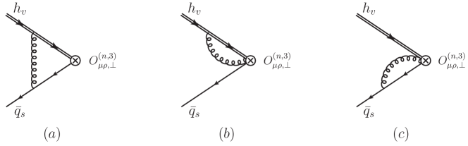
Figure 5: The one-loop HQET diagrams for the renormalization mixing of the evanescent operator $O_{\mu\rho,\perp}^{(n,3)}(\omega^{\prime})$ into the physical operator $O_{\mu\rho,\perp}^{(n,1)}(\omega^{\prime})$.

We proceed to compute the one-loop HQET matrix element of the evanescent operator $O_{\mu\rho,\perp}^{(n,3)}(\omega^{\prime})$ for the determination of the bare amplitude $M_{31}^{(1)\,\rm{off}}$. It is evident that only the diagram (a) in figure 5 can potentially generate the renormalization mixing of the evanescent operator $O_{\mu\rho,\perp}^{(n,3)}(\omega^{\prime})$ into the physical operator $O_{\mu\rho,\perp}^{(n,1)}(\omega^{\prime})$. The corresponding one-loop amplitude can be readily derived with the HQET Feynman rules

$$\langle O_{\mu\rho,\perp}^{(n,3)}(\omega,\omega^{\prime})\rangle^{(1,a)} = i\,g_{s}^{2}\,C_{F}\,\int{d^{D}l\over(2\,\pi)^{D}}\,{1\over[(l+k)^{2}+i0][-v\cdot l+i0][l^{2}+i0]}\,\,\delta(\omega^{\prime}-\omega-\bar{n}\cdot l)$$ (92)

$$\bar{q}_{s}(k)\,\not\!v\,\,(\not l+\not\!k)\,\left[{\not\!n\over 2}\,\,\left(\,{[\gamma_{\rho\perp},\gamma_{\mu\perp}]\over 2}\,\gamma_{5}-i\,\epsilon_{\rho\mu\perp}\,\right)\,\right]\,\,h_{v}\,.$$

Performing the loop-momentum integration and employing the classical equation of motion for the light quark, we observe that the soft gluon correction will not resolve the dynamical structure of the light-ray HQET operator $O_{\mu\rho,\perp}^{(n,3)}(\omega^{\prime})$. Consequently, we obtain

$$M_{31}^{(1)\,\rm{off}}=0\,.$$ (93)

Substituting (93) into (91) yields the final result for the one-loop matching coefficient

$${\cal J}_{\perp,n}^{A,1,(1)}=T_{\perp,n}^{A,1,(1)}-Z_{11}^{(1)}\,\ast{\cal J}_{\perp,n}^{A,1,(0)}\,,$$ (94)

from which we can further write down its explicit expression

$$J_{\perp,-}^{A,(1)} = {\cal J}_{\perp,n}^{A,1,(1)}={\alpha_{s}\,C_{F}\over 4\,\pi}\,\bigg{[}2\,\ln^{2}{\mu^{2}\over n\cdot p\,(\omega-\bar{n}\cdot p)}+\,3\,\ln{\mu^{2}\over n\cdot p\,(\omega-\bar{n}\cdot p)}-{\pi^{2}\over 3}+7\bigg{]}\,\,{\cal J}_{\perp,n}^{A,1,(0)}\,,\hskip 14.22636pt$$

$$J_{\perp,+}^{A,(1)} = {\cal J}_{\perp,\bar{n}}^{A,1,(1)}=0\,.$$ (95)

It needs to point out that the absence of the HQET operator mixing between $O_{\mu\rho,\perp}^{(n,3)}(\omega^{\prime})$ and $O_{\mu\rho,\perp}^{(n,1)}(\omega^{\prime})$ under renormalization arises from the heavy quark spin symmetry, in contrast to the counterpart collinear operator mixing pattern under the radiative correction [61].

3.3.2 SCET factorization for $\Pi_{\mu\nu\rho,\perp}^{B}(p,q)$

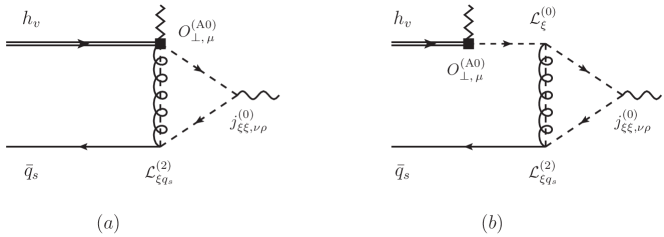
Figure 6: Diagrammatical representation of the vacuum-to-$B$-meson correlation function $\Pi_{\mu\nu\rho,\perp}^{B}(p,q)$ defined with the ${\rm A0}$-type SCET operator $O_{\perp,\,\mu}^{\rm{(A0)}}=\left(\bar{\xi}\,W_{c}\right)\,\gamma_{5}\,\gamma_{\mu\,\perp}\,h_{v}$, the leading power interpolating current $j_{\xi\xi,\nu\rho}^{(0)}$ and the subleading power SCET Lagrangian ${\cal L}_{\xi q_{s}}^{(2)}$.

For the sake of determining the jet functions $J_{\perp,\pm}^{B}$ entering the SCET factorization formula (73), we consider the following partonic matrix element

$$F_{\mu\rho,\perp}^{B}(p,q) = \int d^{4}x\,e^{ip\cdot x}\,\int d^{4}y\,\,$$ (96)

$$\left\langle 0\left|{\rm T}\left\{\bar{\xi}(x)\,\,{\not\!n\over 2}\,\gamma_{\rho\,\perp}\,\xi(x),\,\,i\,{\cal L}_{\xi q_{s}}^{(2)}(y),\,\,\left(\bar{\xi}\,W_{c}\right)(0)\,\gamma_{5}\,\gamma_{\mu\,\perp}\,h_{v}(0)\,\right\}\right|\bar{q}_{s}(k)\,h_{v}\right\rangle.$$

Applying the SCET Feynman rules we can observe that the contribution from the diagram (a) displayed in figure 6 can be read from the result of the corresponding matrix element (33) for the effective currents related to the longitudinally polarized vector meson

$$F_{\mu\rho,\perp}^{B,(a)}(p,q) = {\alpha_{s}\,C_{F}\over 2\,\pi}\,{\bar{n}\cdot p-\omega\over\omega}\,\left[{1\over\epsilon}+\ln{\mu^{2}\over n\cdot p\,(\omega-\bar{n}\cdot p)}+{1\over 2}\,\left({\bar{n}\cdot p-\omega\over\bar{n}\cdot p}\right)+1\right]$$ (97)

$$\times\,\ln\left({\bar{n}\cdot p-\omega\over\bar{n}\cdot p}\right)\,F_{\mu\rho,\perp,\rm{LO}}^{A}(p,q).$$

Evaluating the $\rm{SCET_{I}}$ diagram (b) in figure 6 leads to

$$F_{\mu\rho,\perp}^{B,(b)}(p,q) = g_{s}^{2}\,C_{F}\,\int{d^{D}l\over(2\pi)^{D}}\,\int{d^{D}L\over(2\pi)^{D}}\frac{n\cdot L\,\,n\cdot(p+L)\,\,n\cdot(p+L+l)}{[L^{2}+i0][(p+L)^{2}+i0][(p+L+l)^{2}+i0][l^{2}+i0]}$$ (98)

$$\bar{q}_{s}(k)\,\bigg{\{}(2\,\pi)^{4}\,\delta^{4}(l+L+k)\,\left[\bar{n}^{\alpha}+\gamma_{\perp}^{\alpha}\,{\not\!L_{\perp}\over n\cdot L}+{n^{\alpha}\over n\cdot l}\,{L^{2}\over n\cdot L}\right]\,{\not\!n\over 2}$$

$$+\,k_{\perp\,\beta}\,\partial_{\perp}^{\beta}\,\left[(2\,\pi)^{4}\,\delta^{4}(l+L+k)\right]\,\left[\gamma_{\perp}^{\alpha}-{\not\!L_{\perp}\over n\cdot L}\,n^{\alpha}\right]\,\bigg{\}}$$

$$\gamma_{\rho\perp}\,\left[\bar{n}_{\alpha}+{\gamma_{\alpha\,\perp}\,(\not\!L_{\perp}+\not l_{\perp})\over n\cdot(p+L+l)}+{\not\!L_{\perp}\,\gamma_{\alpha\perp}\over n\cdot(p+L)}-{L_{\perp}^{2}+\not\!L_{\perp}\,\not l_{\perp}\over n\cdot(p+L)\,n\cdot(p+L+l)}\,n_{\alpha}\right]$$

$$\,\,\times\,{\not\!\bar{n}\over 2}\,\gamma_{5}\,\gamma_{\mu\perp}\,h_{v}\,,\hskip 14.22636pt$$

whose result cannot be extracted directly from the counterpart longitudinal matrix element displayed in (35). Implementing the Dirac algebra reduction in the $D$-dimensional space-time and performing the loop momentum integration, we obtain

$$F_{\mu\rho,\perp}^{B,(b)}(p,q) = {\alpha_{s}\,C_{F}\over 4\,\pi}\,\,\bigg{\{}-{2\over\epsilon^{2}}+{1\over\epsilon}\,\left[-2\,\ln\left({\mu^{2}\over n\cdot p\,(\omega-\bar{n}\cdot p)}\right)+\,2\,\,{\ln(1+\eta)\over\eta}-4\right]$$ (99)

$$-\ln^{2}\left({\mu^{2}\over n\cdot p\,(\omega-\bar{n}\cdot p)}\right)+\ln\left({\mu^{2}\over n\cdot p\,(\omega-\bar{n}\cdot p)}\right)\,\left[2\,\,{\ln(1+\eta)\over\eta}-4\right]$$

$$+\,{1\over\eta}\,\ln^{2}(1+\eta)+{4\over\eta}\,\ln(1+\eta)+{\pi^{2}\over 6}-8\bigg{\}}\,\,F_{\mu\rho,\perp,\rm{LO}}^{A}(p,q).$$

Adding up the contributions from these two diagrams and performing the infrared subtraction with the evanescent operator approach, the jet functions $J_{\perp,\pm}^{B}$ can be determined as follows

$$J_{\perp,-}^{B} = {\alpha_{s}\,C_{F}\over 4\,\pi}\,\bigg{[}-\ln^{2}\left({\mu^{2}\over n\cdot p\,(\omega-\bar{n}\cdot p)}\right)+\ln\left({\mu^{2}\over n\cdot p\,(\omega-\bar{n}\cdot p)}\right)\,\left[-2\,\,\ln(1+\eta)-4\right]$$

$$-\ln^{2}(1+\eta)+\left({2\over\eta}-2\right)\,\ln(1+\eta)+{\pi^{2}\over 6}-8\bigg{]}\,\,{\cal J}_{\perp,n}^{A,1,(0)}\,,$$

$$J_{\perp,+}^{B} = 0\,,$$ (100)

which are consistent with the previous results obtained in [26], employing the momentum-space projector for the $B$-meson LCDA in the $D$ dimensional space-time.

3.3.3 SCET factorization for $\Pi_{\mu\nu\rho,\perp}^{C}(p,q)$

We proceed to determine the light-quark-mass induced jet functions $J_{\perp,\pm}^{C}$ appearing in the SCET factorization formula (73) by investigating the partonic matrix element

$$F_{\mu\rho,\perp}^{C}(p,q)=\int d^{4}x\,e^{ip\cdot x}\,\int d^{4}y\,\,\int d^{4}z\,\,$$

$$\hskip 14.22636pt\left\langle 0\left|{\rm T}\left\{\bar{\xi}(x)\,\,{\not\!n\over 2}\,\gamma_{\rho\,\perp}\,\xi(x),\,\,i\,{\cal L}_{\xi q_{s}}^{(1)}(y),\,\,i\,{\cal L}_{\xi m}^{(1)}(z),\,\,\left(\bar{\xi}\,W_{c}\right)(0)\,\gamma_{5}\,\gamma_{\mu\,\perp}\,h_{v}(0)\,\right\}\right|\bar{q}_{s}(k)\,h_{v}\right\rangle.\hskip 28.45274pt$$ (101)

Computing the tree-level contribution to $F_{\mu\rho,\perp}^{C}$ with the SCET Feynman rules leads to

$$F_{\mu\rho,\perp}^{C}(p,q) = {m\over n\cdot p}\,{g_{s}^{2}\,C_{F}\over\bar{n}\cdot p-\omega}\,\,\bar{q}_{s}(k)\,\gamma_{\rho\perp}\,\gamma_{\mu\perp}\,{\not\!\bar{n}\over 2}\,\gamma_{5}\,h_{v}\,\,\int{d^{D}l\over(2\pi)^{D}}\,$$ (102)

$${(D-4)\,(n\cdot l)^{2}\over[n\cdot l\,\bar{n}\cdot(l+k)+l_{\perp}^{2}+i0][n\cdot(p-l)\,\bar{n}\cdot(p-l-k)+l_{\perp}^{2}+i0][l^{2}+i0]}\,,\hskip 14.22636pt$$

which vanishes in the four dimensional space-time in contrast to the result of the counterpart longitudinal matrix element as displayed in (39). The corresponding jet functions $J_{\perp,\pm}^{C}$ can therefore be determined as

$$J_{\perp,+}^{C}=J_{\perp,-}^{C}={\cal O}(\alpha_{s}^{2}).$$ (103)

An interesting consequence from such observation is that the light-quark-mass corrections to the radiative leptonic decay amplitudes of $B\to\gamma\ell\nu_{\ell}$ and $B_{s}\to\gamma\ell\bar{\ell}$ will not give rise to the leading-power contribution in the heavy quark expansion, at least, at ${\cal O}(\alpha_{s})$.

Substituting the derived jet functions (95), (100) and (103) into the SCET factorization formula (73), we can readily write down

$$\Pi_{\mu\nu\rho,\perp}(p,q) = {\tilde{f}_{B}(\mu)\,m_{B}\over 2}\,\int_{0}^{+\infty}\,{d\omega\over\bar{n}\cdot p-\omega+i0}\,\,\left[1+{\alpha_{s}\,C_{F}\over 4\,\pi}\,\hat{J}_{\perp,-}^{(\rm{A0})}\left({\mu^{2}\over n\cdot p\,\omega},{\omega\over\bar{n}\cdot p}\right)\right]\,\phi_{B}^{-}(\omega,\mu)\,$$ (104)

$$\,g_{\mu\rho\,\perp}\,\,\bar{n}_{\nu}\,+{\cal O}(\alpha_{s}^{2})\,,$$

where the renormalized one-loop jet function $\hat{J}_{\perp,-}^{(\rm{A0})}$ reads

$$\hat{J}_{\perp,-}^{(\rm{A0})} = \ln^{2}\left({\mu^{2}\over n\cdot p\,(\omega-\bar{n}\cdot p)}\right)-2\,\ln\left({\mu^{2}\over n\cdot p\,(\omega-\bar{n}\cdot p)}\right)\,\ln(1+\eta)-\ln\left({\mu^{2}\over n\cdot p\,(\omega-\bar{n}\cdot p)}\right)$$ (105)

$$-\ln^{2}(1+\eta)+\left({2\over\eta}-2\right)\,\ln(1+\eta)-{\pi^{2}\over 6}-1\,.$$

The spectral representation of the factorization formula (104) can be further derived with the explicit expressions of the various dispersion integrals displayed in [20]

$$\Pi_{\mu\nu\rho,\perp}(p,q)=-{\tilde{f}_{B}(\mu)\,m_{B}\over 2}\,\int_{0}^{+\infty}\,{d\omega^{\prime}\over\omega^{\prime}-\bar{n}\cdot p-i0}\,\,\tilde{\phi}_{B,\rm{eff}}^{-}(\omega^{\prime},\mu)\,\,g_{\mu\rho\,\perp}\,\,\bar{n}_{\nu}\,+{\cal O}(\alpha_{s}^{2})\,,$$ (106)

where we have introduced the “effective” $B$-meson distribution amplitude $\tilde{\phi}_{B,\rm{eff}}^{-}$ for brevity

$$\tilde{\phi}_{B,\rm{eff}}^{-}(\omega^{\prime},\mu)$$

$$=\phi_{B}^{-}(\omega^{\prime},\mu)+{\alpha_{s}\,C_{F}\over 4\,\pi}\,\bigg{\{}\int_{0}^{\omega^{\prime}}d\omega\,\left[{2\over\omega-\omega^{\prime}}\,\left(\ln{\mu^{2}\over n\cdot p\,\omega^{\prime}}-2\,\ln{\omega^{\prime}-\omega\over\omega^{\prime}}-{1\over 2}\right)\right]_{\oplus}\,\phi_{B}^{-}(\omega,\mu)$$

$$\hskip 14.22636pt-\int_{\omega^{\prime}}^{\infty}\,d\omega\,\bigg{[}\ln^{2}{\mu^{2}\over n\cdot p\,\omega^{\prime}}-\ln{\mu^{2}\over n\cdot p\,\omega^{\prime}}-\left(2\,\ln{\mu^{2}\over n\cdot p\,\omega^{\prime}}+4\right)\,\ln{\omega-\omega^{\prime}\over\omega^{\prime}}+2\,\ln{\omega\over\omega^{\prime}}$$

$$\hskip 71.13188pt+\,{\pi^{2}\over 6}-1\bigg{]}\,\,{d\phi_{B}^{-}(\omega,\mu)\over d\omega}\bigg{\}}\,.$$ (107)

Matching the SCET factorization formula (106) with the hadronic dispersion relation for the vacuum-to-$B$-meson correlation function $\Pi_{\mu\nu\rho,\perp}$

$$\Pi_{\mu\nu\rho,\perp}(p,q)$$

$$=\left[-{f_{V,\perp}(\nu)\,n\cdot p\over m_{V}^{2}/n\cdot p-\bar{n}\cdot p-i0}\,{\xi_{\perp}(n\cdot p)\over 2}\,+\int_{\omega_{s}}^{+\infty}\,{d\omega^{\prime}\over\omega^{\prime}-\bar{n}\cdot p-i0}\,\,\rho^{h}_{\perp}(\omega^{\prime},n\cdot p)\right]\,g_{\mu\rho\,\perp}\,\,\bar{n}_{\nu}\,,\hskip 22.76228pt$$ (108)

and implementing the NLL resummation for the enhanced logarithms of $\mu/\mu_{0}$, we obtain the following SCET sum rules for the form factor $\xi_{\perp}(n\cdot p)$ at ${\cal O}(\alpha_{s})$

$$\xi_{\perp}(n\cdot p)={U_{2}(\mu_{h2},\mu)\,\tilde{f}_{B}(\mu_{h2})\over f_{V,\perp}(\nu)}\,{m_{B}\over n\cdot p}\,\int_{0}^{\omega_{s}}\,d\omega^{\prime}\,{\rm exp}\left[-{n\cdot p\,\omega^{\prime}-m_{V}^{2}\over n\cdot p\,\omega_{M}}\right]\,\,\tilde{\phi}_{B,\rm{eff}}^{-}(\omega^{\prime},\mu)\,.$$ (109)

The renormalization-scale dependent transverse decay constant of the vector meson $f_{V,\perp}$ is defined as follows

$$c_{V}\,\,\langle V(p,\epsilon^{\ast})|j_{\nu\rho}|0\rangle=-\,i\,f_{V,\perp}(\nu)\,\,p_{\nu}\,\,\epsilon^{\ast}_{\rho\perp}(p)\,,$$ (110)

where the corresponding RG evolution equation can be written as

$${d\over d\ln\nu}\,f_{V,\perp}(\nu)=\gamma_{T}(\alpha_{s})\,\,f_{V,\perp}(\nu)\,,\qquad\gamma_{T}(\alpha_{s})=\sum_{n=0}^{\infty}\,\left({\alpha_{s}\over 4\,\pi}\right)^{n+1}\,\gamma_{T,n}\,,$$ (111)

with the first two expansion coefficients [62]

$$\gamma_{T,0}=-2\,C_{F}\,,\qquad\gamma_{T,1}=C_{F}\,\left[19\,C_{F}-{257\over 9}\,C_{A}+{52\over 9}\,\left(n_{l}+1\right)\,T_{F}\right]\,.$$ (112)

It is evident from the definitions of the $\rm{A0}$-type SCET form factors (2) that $\xi_{\perp}(n\cdot p)$ is independent of the QCD renormalization scale $\nu$ of the transverse decay constant $f_{V,\perp}(\nu)$. In order to demonstrate such argument from the obtained $B$-meson LCSR displayed in (109), we need to distinguish the renormalization scale $\nu$ for the tensor interpolating current of the vector meson $j_{\nu\rho}$ from the factorization scale $\mu$ that is related to the RG evolution of the light-cone HQET operators. To this end, we decompose the one-loop jet function $\hat{J}_{\perp,-}^{(\rm{A0})}$ entering the factorization formula (104) into the following two pieces

$$\hat{J}_{\perp,-}^{(\rm{A0})}\left({\mu^{2}\over n\cdot p\,\omega},{\omega\over\bar{n}\cdot p},\nu\right)=\hat{J}_{\perp,-}^{(\rm{A0})}\left({\mu^{2}\over n\cdot p\,\omega},{\omega\over\bar{n}\cdot p}\right)+\delta\hat{J}_{\perp,-}^{(\rm{A0})}\left({\mu^{2}\over n\cdot p\,\omega},{\omega\over\bar{n}\cdot p},\nu\right)\,,$$ (113)

where the QCD scale $\nu$ dependence of the second term on the right-hand side is determined by the RG evolution equation for the tensor current

$${d\over d\ln\nu}\,\delta\hat{J}_{\perp,-}^{(\rm{A0})}\left({\mu^{2}\over n\cdot p\,\omega},{\omega\over\bar{n}\cdot p},\nu\right)=\gamma_{T}(\alpha_{s})\,\,\delta\hat{J}_{\perp,-}^{(\rm{A0})}\left({\mu^{2}\over n\cdot p\,\omega},{\omega\over\bar{n}\cdot p},\nu\right)\,.$$ (114)

Employing the consistency condition of the newly defined function for $\nu=\mu$

$$\delta\hat{J}_{\perp,-}^{(\rm{A0})}\left({\mu^{2}\over n\cdot p\,\omega},{\omega\over\bar{n}\cdot p},\nu=\mu\right)=0\,,$$ (115)

it is straightforward to write down the solution to (114)

$$\delta\hat{J}_{\perp,-}^{(\rm{A0})}\left({\mu^{2}\over n\cdot p\,\omega},{\omega\over\bar{n}\cdot p},\nu\right)={\alpha_{s}(\mu)\over 4\,\pi}\,\gamma_{T,0}\,\ln\left({\nu\over\mu}\right)+{\cal O}(\alpha_{s}^{2})\,.$$ (116)

The resulting hard-collinear function $\hat{J}_{\perp,-}^{(\rm{A0})}$ is therefore given by

$$\hat{J}_{\perp,-}^{(\rm{A0})}\left({\mu^{2}\over n\cdot p\,\omega},{\omega\over\bar{n}\cdot p},\nu\right)$$

$$=\ln^{2}\left({\mu^{2}\over n\cdot p\,(\omega-\bar{n}\cdot p)}\right)-2\,\ln\left({\mu^{2}\over n\cdot p\,(\omega-\bar{n}\cdot p)}\right)\,\ln(1+\eta)$$

$$\hskip 14.22636pt-\ln\left({\nu^{2}\over n\cdot p\,(\omega-\bar{n}\cdot p)}\right)-\ln^{2}(1+\eta)+\left({2\over\eta}-2\right)\,\ln(1+\eta)-{\pi^{2}\over 6}-1\,.$$ (117)

As a consequence, the “effective” distribution amplitude entering the SCET sum rules for $\xi_{\perp}(n\cdot p)$ with the two scales $\mu$ and $\nu$ distinct from each other is given by

$$\tilde{\phi}_{B,\rm{eff}}^{-}(\omega^{\prime},\mu,\nu)$$

$$=\phi_{B}^{-}(\omega^{\prime},\mu)+{\alpha_{s}\,C_{F}\over 4\,\pi}\,\bigg{\{}\int_{0}^{\omega^{\prime}}d\omega\,\left[{2\over\omega-\omega^{\prime}}\,\left(\ln{\mu^{2}\over n\cdot p\,\omega^{\prime}}-2\,\ln{\omega^{\prime}-\omega\over\omega^{\prime}}-{1\over 2}\right)\right]_{\oplus}\,\phi_{B}^{-}(\omega,\mu)$$

$$\hskip 14.22636pt-\int_{\omega^{\prime}}^{\infty}\,d\omega\,\bigg{[}\ln^{2}{\mu^{2}\over n\cdot p\,\omega^{\prime}}-\ln{\nu^{2}\over n\cdot p\,\omega^{\prime}}-\left(2\,\ln{\mu^{2}\over n\cdot p\,\omega^{\prime}}+4\right)\,\ln{\omega-\omega^{\prime}\over\omega^{\prime}}+2\,\ln{\omega\over\omega^{\prime}}$$

$$\hskip 71.13188pt+\,{\pi^{2}\over 6}-1\bigg{]}\,\,{d\phi_{B}^{-}(\omega,\mu)\over d\omega}\bigg{\}}\,.$$ (118)

3.4 The $B$-meson LCSR for $\Xi_{\perp}(\tau,n\cdot p)$

Now we turn to construct the sum rules for the $\rm{B}$-type SCET form factor $\Xi_{\perp}(\tau,n\cdot p)$ with the following vacuum-to-$B$-meson correlation function

$$\widetilde{\Pi}_{\mu\nu\rho,\perp}(p,q,\tau) = {n\cdot p\over 2\,\pi}\,\int d^{4}x\,e^{ip\cdot x}\,\int dr\,e^{-in\cdot p\,\tau\,r}\,$$ (119)

$$\langle 0|{\rm T}\left\{j_{\nu\rho}(x),\,\,\left(\bar{\xi}\,W_{c}\right)(0)\,\gamma_{5}\,\,\gamma_{\mu\perp}\,\,(W_{c}^{\dagger}\,\,i\not\!\!D_{c,\,\perp}\,W_{c})(r\,n)\,\,h_{v}(0)\,\right\}|\bar{B}_{v}\rangle\,.$$

Employing the $\rm{SCET_{I}}$ representation (70) of the interpolating current for the transversely polarized vector meson, it is straightforward to identify the leading power contribution of the correlation function (119)

$$\widetilde{\Pi}_{\mu\nu\rho,\perp}(p,q,\tau) = {n\cdot p\over 2\,\pi}\,\int d^{4}x\,e^{ip\cdot x}\,\,\int d^{4}y\,\int dr\,e^{-in\cdot p\,\tau\,r}\,\bigg{\langle}0\bigg{|}{\rm T}\bigg{\{}j_{\xi\xi,\nu\rho}^{(0)}(x),\,\,i\,{\cal L}_{\xi q_{s}}^{(1)}(y)\,,$$ (120)

$$\left(\bar{\xi}\,W_{c}\right)(0)\,\gamma_{5}\,\,\gamma_{\mu\perp}\,\,(W_{c}^{\dagger}\,\,i\not\!\!D_{c,\,\perp}\,W_{c})(r\,n)\,\,h_{v}(0)\,\bigg{\}}\bigg{|}\bar{B}_{v}\bigg{\rangle}\,.$$

Performing the perturbative matching of the $\rm{SCET_{I}}$ matrix element onto HQET yields the soft-collinear factorization formula

$$\widetilde{\Pi}_{\mu\nu\rho,\perp}(p,q,\tau)={\tilde{f}_{B}(\mu)\,m_{B}\over 2}\,\sum_{m=\pm}\,\int_{0}^{+\infty}\,d\omega\,\tilde{J}_{\perp,m}\left({\mu^{2}\over n\cdot p\,\omega},{\omega\over\bar{n}\cdot p},\tau\right)\,\phi_{B}^{m}(\omega,\mu)\,\,g_{\mu\rho\perp}\,\,\bar{n}_{\nu}.$$ (121)

The short-distance functions $\tilde{J}_{\perp,m}$ can be extracted from the hard-collinear contribution to the partonic matrix element

$$\widetilde{F}_{\mu\nu\rho,\perp}(p,q,\tau) = {n\cdot p\over 2\,\pi}\,\int d^{4}x\,e^{ip\cdot x}\,\,\int d^{4}y\,\int dr\,e^{-in\cdot p\,\tau\,r}\,\,\bigg{\langle}0\bigg{|}{\rm T}\bigg{\{}j_{\xi\xi,\nu\rho}^{(0)}(x),\,\,i\,{\cal L}_{\xi q_{s}}^{(1)}(y)\,,$$ (122)

$$\left(\bar{\xi}\,W_{c}\right)(0)\,\gamma_{5}\,\,\gamma_{\mu\perp}\,\,(W_{c}^{\dagger}\,\,i\not\!D_{c,\,\perp}\,W_{c})(r\,n)\,\,h_{v}(0)\,\bigg{\}}\bigg{|}\bar{q}_{s}(k)\,\,h_{v}\bigg{\rangle}\,.$$

Employing the SCET Feynman rules we can readily derive the tree-level amplitude

$$\widetilde{F}_{\mu\nu\rho,\perp}(p,q,\tau) = g_{s}^{2}\,C_{F}\,\,\bar{q}_{s}(k)\,\left[(D-4)\,\gamma_{\rho\perp}\,\gamma_{\mu\perp}+2\,\gamma_{\mu\perp}\,\gamma_{\rho\perp}\right]\,\,\,{\not\!\bar{n}\over 2}\,\gamma_{5}\,h_{v}\,\,\bar{n}_{\nu}$$ (123)

$$\int{d^{D}l\over(2\pi)^{D}}\,{n\cdot l\,n\cdot(p-l)\,\delta(\tau-n\cdot l/n\cdot p)\over[n\cdot l\,\bar{n}\cdot(l+k)+l_{\perp}^{2}+i0][n\cdot(p-l)\,\bar{n}\cdot(p-l-k)+l_{\perp}^{2}+i0][l^{2}+i0]}\,,\hskip 28.45274pt$$

which can be further computed as follows

$$\widetilde{F}_{\mu\nu\rho,\perp}(p,q,\tau)$$

$$=\left(-i\right)\,{\alpha_{s}\,C_{F}\over 2\,\pi}\,{n\cdot p\over\omega}\,\ln(1+\eta)\,\left[(1-\tau)\,\theta(\tau)\,\theta(1-\tau)\right]\,\,\,\bar{q}_{s}(k)\,\gamma_{\mu\perp}\,\gamma_{\rho\perp}\,{\not\!\bar{n}\over 2}\,\gamma_{5}\,h_{v}\,\,\bar{n}_{\nu}\,.$$ (124)

Applying the perturbative matching relation for the SCET matrix element

$$\widetilde{F}_{\mu\nu\rho,\perp}(p,q,\tau)=(-i)\,\sum_{k=1,2,3}\,{\cal\tilde{J}}_{\perp,\bar{n}}^{A,k}\left({\mu^{2}\over n\cdot p\,\omega^{\prime}},{\omega^{\prime}\over\bar{n}\cdot p},\tau\right)\ast\langle O_{\mu\rho,\perp}^{(\bar{n},k)}(\omega,\omega^{\prime})\rangle\,\,\bar{n}_{\nu}\,,$$ (125)

with the light-cone HQET operators in the momentum space defined by

$$O_{\mu\rho,\perp}^{(\bar{n},1)}(\omega^{\prime}) = {1\over 2\,\pi}\,\int dt\,e^{i\,t\,\omega^{\prime}}\,\left(\bar{q}_{s}Y_{s}\right)(t\,\bar{n})\,\,\left[\,g_{\rho\mu\perp}\,{\not\!\bar{n}\over 2}\,\,\gamma_{5}\,\right]\,\,\left(Y_{s}^{{\dagger}}h_{v}\right)(0)\,,$$

$$O_{\mu\rho,\perp}^{(\bar{n},2)}(\omega^{\prime}) = {1\over 2\,\pi}\,\int dt\,e^{i\,t\,\omega^{\prime}}\,\left(\bar{q}_{s}Y_{s}\right)(t\,\bar{n})\,\,\left[\,i\,\epsilon_{\rho\mu\perp}\,{\not\!\bar{n}\over 2}\,\right]\,\,\left(Y_{s}^{{\dagger}}h_{v}\right)(0)\,,$$

$$O_{\mu\rho,\perp}^{(\bar{n},3)}(\omega^{\prime}) = {1\over 2\,\pi}\,\int dt\,e^{i\,t\,\omega^{\prime}}\,\left(\bar{q}_{s}Y_{s}\right)(t\,\bar{n})\,\,\left[{\not\!\bar{n}\over 2}\,\,\left(\,{[\gamma_{\rho\perp},\gamma_{\mu\perp}]\over 2}\,\gamma_{5}+i\,\epsilon_{\rho\mu\perp}\,\right)\,\right]\,\,\left(Y_{s}^{{\dagger}}h_{v}\right)(0)\,,\hskip 22.76228pt$$ (126)

and implementing the infrared subtraction scheme with the evanescent operator approach described in the previous subsections, the determined jet functions are given by

$$\tilde{J}_{\perp,\,+}={\cal\tilde{J}}_{\perp,\bar{n}}^{A,1}={\alpha_{s}\,C_{F}\over 2\,\pi}\,{n\cdot p\over\omega}\,\ln(1+\eta)\,\left[(1-\tau)\,\theta(\tau)\,\theta(1-\tau)\right]\,,\qquad\tilde{J}_{\perp,\,-}={\cal\tilde{J}}_{\perp,n}^{A,1}=0.\hskip 14.22636pt$$ (127)

Taking advantage of the spectral representation of the factorization formula (121) for the vacuum-to-$B$-meson correlation function $\widetilde{\Pi}_{\mu\nu\rho,\perp}$

$$\widetilde{\Pi}_{\mu\nu\rho,\perp}(p,q,\tau) = {\alpha_{s}\,C_{F}\over 4\,\pi}\,\tilde{f}_{B}(\mu)\,m_{B}\,\left[(1-\tau)\,\theta(\tau)\,\theta(1-\tau)\right]\,$$ (128)

$$\times\,\int_{0}^{\infty}{d\omega^{\prime}\over\omega^{\prime}-\bar{n}\cdot p-i0}\,\left[\int_{\omega^{\prime}}^{\infty}d\omega\,{n\cdot p\over\omega}\,\phi_{B}^{+}(\omega,\mu)\right]\,g_{\mu\rho\perp}\,\,\bar{n}_{\nu}\,,$$

with the aid of the corresponding hadronic dispersion relation

$$\widetilde{\Pi}_{\mu\nu\rho,\perp}(p,q,\tau) = \bigg{[}-{f_{V,\perp}(\nu)\,\,m_{b}\over m_{V}^{2}/n\cdot p-\bar{n}\cdot p-i0}\,\left({n\cdot p\over 2}\right)\,\,\Xi_{\perp}(\tau,n\cdot p)$$ (129)

$$+\int_{\omega_{s}}^{+\infty}\,{d\omega^{\prime}\over\omega^{\prime}-\bar{n}\cdot p-i0}\,\,\tilde{\rho}^{h}_{\perp}(\omega^{\prime},n\cdot p,\tau)\bigg{]}\,g_{\mu\rho\perp}\,\,\bar{n}_{\nu}\,,$$

we obtain the desired sum rules for the non-local form factor $\Xi_{\perp}(\tau,n\cdot p)$ under the parton-hadron duality approximation

$$\Xi_{\perp}(\tau,n\cdot p) = -{\alpha_{s}\,C_{F}\over 2\,\pi}\,{U_{2}(\mu_{h2},\mu)\,\,\tilde{f}_{B}(\mu)\over f_{V,\perp}(\nu)}\,{m_{B}\over m_{b}}\,\,\left[(1-\tau)\,\theta(\tau)\,\theta(1-\tau)\right]\,$$ (130)

$$\times\,\int_{0}^{\omega_{s}}\,d\omega^{\prime}\,{\rm exp}\left[-{n\cdot p\,\omega^{\prime}-m_{V}^{2}\over n\cdot p\,\omega_{M}}\right]\int_{\omega^{\prime}}^{\infty}\,d\omega\,{\phi_{B}^{+}(\omega,\mu)\over\omega}\,+{\cal O}(\alpha_{s}^{2})\,.$$

Comparing the tree-level sum rules for the $\rm{B}$-type SCET form factors $\Xi_{\|,\perp}(\tau,n\cdot p)$ presented in (62) and (130) leads to the following relation

$${\Xi_{\perp}(\tau,n\cdot p)\over\Xi_{\|}(\tau,n\cdot p)}={f_{V,\perp}(\nu)\over f_{V,\|}}\,\,{n\cdot p\over 2\,m_{V}}\,\,+{\cal O}(\alpha_{s}^{2})\,,$$ (131)

which is in precise agreement with the SCET factorization formulae obtained in [42]. It remains to be verified that whether the LCSR calculations of $\Xi_{\|,\perp}(\tau,n\cdot p)$ with the $B$-meson distribution amplitudes can reproduce the already accomplished SCET computations at ${\cal O}(\alpha_{s}^{2})$.

3.5 RG improvement of the hard matching coefficients

Plugging the obtained sum rules for the “effective” form factors (51), (62), (109) and (130) into the $\rm{SCET_{I}}$ factorization formulae (8) gives rise to the explicit expressions of the leading-power contributions to the seven semileptonic $B\to V$ form factors in the heavy quark expansion, which serve as one of the major technical results of our paper. Taking the factorization scale $\mu$ of order $\sqrt{m_{b}\,\Lambda}$, the hard matching functions $C_{i}^{(\rm{A0})}$ and $C_{i}^{(\rm{B1})}$ involve the parametrically enhanced logarithms $\ln(m_{b}/\Lambda)$, which need to be summed up to all orders in perturbation theory at NLL and LL accuracy. To achieve this goal, we will apply the RG evolution equations for these short-distance functions in the momentum space [41, 42]

$${d\over d\ln\mu}\,C_{i}^{(\rm{A0})}(n\cdot p,\mu) = \left[-\Gamma_{\rm cusp}(\alpha_{s})\,\ln\left({\mu\over n\cdot p}\right)+\gamma(\alpha_{s})\right]\,C_{i}^{(\rm{A0})}(n\cdot p,\mu)\,,$$

$${d\over d\ln\mu}\,C_{i}^{(\rm{B1})}(n\cdot p,\tau,\mu) = -\Gamma_{\rm cusp}(\alpha_{s})\,\ln\left({\mu\over n\cdot p}\right)\,C_{i}^{(\rm{B1})}(n\cdot p,\tau,\mu)$$ (132)

$$+\int_{0}^{1}d\tau^{\prime}\,\gamma_{i}^{(\rm{B1})}(\tau^{\prime},\tau)\,C_{i}^{(\rm{B1})}(n\cdot p,\tau^{\prime},\mu)\,,$$

where the anomalous dimension $\gamma(\alpha_{s})$ does not depend on the Dirac structures of the ${\rm A0}$-type SCET currents, however, the non-local evolution kernels $\gamma_{i}^{(\rm{B1})}(\tau^{\prime},\tau)$ are dependent on the spin structures of the ${\rm B1}$-type SCET currents. The general solutions to these RG equations can be written as

$$C_{i}^{(\rm{A0})}(n\cdot p,\mu) = U_{1}(n\cdot p,\mu_{h},\mu)\,C_{i}^{(\rm{A0})}(n\cdot p,\mu_{h})\,,$$ (133)

$$C_{i}^{(\rm{B1})}(n\cdot p,\tau,\mu) = {\rm Exp}\left[-S(n\cdot p,\mu_{h},\mu)\right]\,\int_{0}^{1}d\tau^{\prime}\,U_{i}^{(\rm{B1})}(\tau,\tau^{\prime},\mu_{h},\mu)\,C_{i}^{(\rm{B1})}(n\cdot p,\tau^{\prime},\mu_{h})\,,\hskip 14.22636pt$$ (134)

where the NLL approximation of the evolution function $U_{1}$ and the LL expansion of the $S$ function can be found in [55] and [42], respectively. As the tree-level expressions of the ${\rm B1}$-type hard functions $C_{i}^{(\rm{B1})}(n\cdot p,\tau,\mu_{h})$ displayed in the Appendix A are independent of the $\tau$ variable, the solution to the corresponding RG equation can be further reduced as

$$C_{i,\,\rm{LL}}^{(\rm{B1})}(n\cdot p,\tau,\mu) = {\rm Exp}\left[-S(n\cdot p,\mu_{h},\mu)\right]\,U_{i}^{(\rm{B1})}(\tau,\mu_{h},\mu)\,C_{i,\,\rm{LO}}^{(\rm{B1})}(n\cdot p,\mu_{h})\,,$$ (135)

with the newly defined evolution function

$$U_{i}^{(\rm{B1})}(\tau,\mu_{h},\mu)=\int_{0}^{1}d\tau^{\prime}\,U_{i}^{(\rm{B1})}(\tau,\tau^{\prime},\mu_{h},\mu)\,.$$ (136)

An approximate solution to $U_{i}^{(\rm{B1})}(\tau,\mu_{h},\mu)$ (better than 1%) at the LL accuracy reads

$$U_{i,\,\rm{app}}^{(\rm{B1})}(\tau,\mu_{h},\mu)=\left({\alpha_{s}(\mu)\over\alpha_{s}(\mu_{h})}\right)^{-\gamma_{i}^{(\rm B1)}(\tau)/(2\,\beta_{0})}\,,$$ (137)

with the explicit expressions of $\gamma_{i}^{(\rm B1)}(\tau)$ given by [42]

$$\gamma_{\|}^{(\rm B1)}(\tau) = -C_{F}+4\,\left(C_{F}-{C_{A}\over 2}\right)\,{\ln\bar{\tau}\over\tau}\,,$$

$$\gamma_{\perp}^{(\rm B1)}(\tau) = -C_{F}\,\left[{4\,\tau\ln\tau\over\bar{\tau}}+1\right]+4\,\left(C_{F}-{C_{A}\over 2}\right)\,\left[{1+\tau\over\tau}\,\ln\bar{\tau}+{\tau\,\ln\tau\over\bar{\tau}}\right]\,.$$ (138)

The large logarithmic resummation improved SCET factorization formulae can then be deduced by substituting the solutions (133) and (135) into (8) with

$$i = \|\hskip 14.22636pt{\rm for}\hskip 8.5359ptC_{f_{0}}^{(\rm B1)},\,\,C_{f_{+}}^{(\rm B1)},\,\,C_{f_{T}}^{(\rm B1)}\,,$$

$$i = \perp\hskip 8.5359pt{\rm for}\hskip 8.5359ptC_{V}^{(\rm B1)},\,\,C_{T_{1}}^{(\rm B1)}\,.$$ (139)

4 The higher-twist corrections to $B\to V$ form factors

We are now in a position to compute the higher-twist corrections to the semileptonic $B\to V$ form factors from both the two-particle and three-particle $B$-meson distribution amplitudes at tree level by employing the LCSR approach. To this end, we will need to establish the QCD factorization formulae for the following vacuum-to-$B$-meson correlation functions

$$\hat{\Pi}_{\mu,\|}^{(a)}(p,q) = \int d^{4}x\,\,e^{ip\cdot x}\,\,\langle 0|{\rm T}\,\left\{j_{\|}^{V}(x),\,\,\bar{q}(0)\,\Gamma_{\mu}^{(a)}\,b(0)\right\}|\bar{B}(p+q)\rangle\,,$$

$$\hat{\Pi}_{\delta\mu,\perp}^{(a)}(p,q) = \int d^{4}x\,\,e^{ip\cdot x}\,\,\langle 0|{\rm T}\,\left\{j_{\delta,\perp}^{V}(x),\,\,\bar{q}(0)\,\Gamma_{\mu}^{(a)}\,b(0)\right\}|\bar{B}(p+q)\rangle\,,$$ (140)

where the interpolating QCD currents for the longitudinally and transversely polarized vector mesons are given by

$$j_{\|}^{V}(x)=\bar{q}^{\prime}(x)\,{\not\!n\over 2}\,q(x)\,,\qquad j_{\delta,\perp}^{V}(x)=\bar{q}^{\prime}(x)\,{\not\!n\over 2}\,\gamma_{\delta\perp}\,q(x)\,,$$ (141)

and the Dirac structures of the heavy-to-light transition currents under discussion are

$$\Gamma_{\mu}^{(a)}\in\left\{\gamma_{\mu}\,(1-\gamma_{5}),\qquad\,i\,\sigma_{\mu\nu}\,(1+\gamma_{5})\,q^{\nu}\right\}\,.$$ (142)

Employing the light-cone expansion of the quark propagator in the background gluon filed up to the gluon field strength terms without the covariant derivatives [63] (see also [64] for an update for the massive quark case)

$$\langle 0|{\rm T}\,\{\bar{q}(x),q(0)\}|0\rangle\supset i\,g_{s}\,\int_{0}^{\infty}\,\,{d^{4}l\over(2\pi)^{4}}\,e^{-i\,l\cdot x}\,\int_{0}^{1}\,du\,\left[{u\,x_{\mu}\,\gamma_{\nu}\over l^{2}-m^{2}}-\frac{(\not l+m)\,\sigma_{\mu\nu}}{2\,(l^{2}-m^{2})^{2}}\right]\,G^{\mu\nu}(u\,x),\hskip 22.76228pt$$ (143)

with $G_{\mu\nu}=G_{\mu\nu}^{a}\,T^{a}=[D_{\mu},A_{\nu}]$, and applying the general parametrization of the vacuum-to-$B$-meson matrix element of the three-body light-ray HQET operator [43] (see [44] for the original but incomplete parametrization in terms of four independent distribution amplitudes)

$$\langle 0|\bar{q}_{\alpha}(z_{1}\,\bar{n})\,g_{s}\,G_{\mu\nu}(z_{2}\,\bar{n})\,h_{v\,\beta}(0)|\bar{B}_{v}\rangle$$

$$={\tilde{f}_{B}(\mu)\,m_{B}\over 4}\,\bigg{[}(1+\not v)\,\bigg{\{}(v_{\mu}\gamma_{\nu}-v_{\nu}\gamma_{\mu})\,\left[\Psi_{A}(z_{1},z_{2},\mu)-\Psi_{V}(z_{1},z_{2},\mu)\right]-i\,\sigma_{\mu\nu}\,\Psi_{V}(z_{1},z_{2},\mu)$$

$$\hskip 11.38092pt-(\bar{n}_{\mu}\,v_{\nu}-\bar{n}_{\nu}\,v_{\mu})\,X_{A}(z_{1},z_{2},\mu)+(\bar{n}_{\mu}\,\gamma_{\nu}-\bar{n}_{\nu}\,\gamma_{\mu})\,\left[W(z_{1},z_{2},\mu)+Y_{A}(z_{1},z_{2},\mu)\right]$$

$$\hskip 11.38092pt+\,i\,\epsilon_{\mu\nu\alpha\beta}\,\bar{n}^{\alpha}\,v^{\beta}\,\gamma_{5}\,\tilde{X}_{A}(z_{1},z_{2},\mu)-\,i\,\epsilon_{\mu\nu\alpha\beta}\,\bar{n}^{\alpha}\,\gamma^{\beta}\,\gamma_{5}\,\tilde{Y}_{A}(z_{1},z_{2},\mu)$$

$$\hskip 11.38092pt-\,(\bar{n}_{\mu}\,v_{\nu}-\bar{n}_{\nu}\,v_{\mu})\,\not\bar{n}\,W(z_{1},z_{2},\mu)+\,(\bar{n}_{\mu}\,\gamma_{\nu}-\bar{n}_{\nu}\,\gamma_{\mu})\,\not\bar{n}\,Z(z_{1},z_{2},\mu)\bigg{\}}\,\gamma_{5}\bigg{]}_{\beta\,\alpha}\,,$$ (144)

we can readily derive the three-particle higher twist corrections to the aforementioned correlation functions at LO in ${\cal O}(\alpha_{s})$

$$\hat{\Pi}_{\mu,\|}^{(V-A),\,\rm{3P}}(p,q) = -{\tilde{f}_{B}(\mu)\,m_{B}\over 2\,n\cdot p}\,\int_{0}^{\infty}\,d\omega_{1}\,\int_{0}^{\infty}\,d\omega_{2}\,\int_{0}^{1}\,du\,{1\over[\bar{n}\cdot p-\omega_{1}-u\,\omega_{2}+i0]^{2}}\,$$

$$\times\,\bigg{\{}\bar{n}_{\mu}\,\left[\rho_{\bar{n},\|,\,\rm{LP}}^{(V-A),\,\rm{3P}}(u,\omega_{1},\omega_{2})+{m\over n\cdot p}\,\rho_{\bar{n},\|,\,\rm{NLP}}^{(V-A),\,\rm{3P}}(u,\omega_{1},\omega_{2})\right]$$

$$\hskip 22.76228pt+\,n_{\mu}\,\left[\rho_{n,\|,\,\rm{LP}}^{(V-A),\,\rm{3P}}(u,\omega_{1},\omega_{2})+{m\over n\cdot p}\,\rho_{n,\|,\,\rm{NLP}}^{(V-A),\,\rm{3P}}(u,\omega_{1},\omega_{2})\right]\bigg{\}},$$

$$\hat{\Pi}_{\delta\mu,\perp}^{(V-A),\,\rm{3P}}(p,q) = -{\tilde{f}_{B}(\mu)\,m_{B}\over 2\,n\cdot p}\,\int_{0}^{\infty}\,d\omega_{1}\,\int_{0}^{\infty}\,d\omega_{2}\,\int_{0}^{1}\,du\,{1\over[\bar{n}\cdot p-\omega_{1}-u\,\omega_{2}+i0]^{2}}$$

$$\times\,\bigg{\{}\left[g_{\delta\mu\perp}+i\,\epsilon_{\delta\mu\perp}\right]\,\rho_{\perp,\,\rm{LP}}^{(V-A),\,\rm{3P}}(u,\omega_{1},\omega_{2})+{m\over n\cdot p}\,\left[g_{\delta\mu\perp}-i\,\epsilon_{\delta\mu\perp}\right]\,\rho_{\perp,\,\rm{NLP}}^{(V-A),\,\rm{3P}}(u,\omega_{1},\omega_{2})\bigg{\}}\,,$$

$$\hat{\Pi}_{\mu,\|}^{(T+\tilde{T}),\,\rm{3P}}(p,q) = {\tilde{f}_{B}(\mu)\,m_{B}\over 4\,n\cdot p}\,\int_{0}^{\infty}\,d\omega_{1}\,\int_{0}^{\infty}\,d\omega_{2}\,\int_{0}^{1}\,du\,{1\over[\bar{n}\cdot p-\omega_{1}-u\,\omega_{2}+i0]^{2}}\,$$

$$\times\,\left(\bar{n}_{\mu}\,n\cdot q-n_{\mu}\,\bar{n}\cdot q\right)\,\,\left[\rho_{\|,\,\rm{LP}}^{(T+\tilde{T}),\,\rm{3P}}(u,\omega_{1},\omega_{2})+{m\over n\cdot p}\,\rho_{\|,\,\rm{NLP}}^{(T+\tilde{T}),\,\rm{3P}}(u,\omega_{1},\omega_{2})\right]\,,$$

$$\hat{\Pi}_{\delta\mu,\perp}^{(T+\tilde{T}),\,\rm{3P}}(p,q) = {\tilde{f}_{B}(\mu)\,m_{B}\over 2\,n\cdot p}\,\,\bar{n}\cdot q\,\int_{0}^{\infty}\,d\omega_{1}\,\int_{0}^{\infty}\,d\omega_{2}\,\int_{0}^{1}\,du\,{1\over[\bar{n}\cdot p-\omega_{1}-u\,\omega_{2}+i0]^{2}}\,$$

$$\times\,\bigg{\{}\left[g_{\delta\mu\perp}+i\,\epsilon_{\delta\mu\perp}\right]\,\rho_{\perp,\,\rm{LP}}^{(T+\tilde{T}),\,\rm{3P}}(u,\omega_{1},\omega_{2})+{m\,n\cdot q\over 2\,p\cdot q}\,\left[g_{\delta\mu\perp}-i\,\epsilon_{\delta\mu\perp}\right]\,\rho_{\perp,\,\rm{NLP}}^{(T+\tilde{T}),\,\rm{3P}}(u,\omega_{1},\omega_{2})\bigg{\}}.$$

The explicit expressions of the invariant functions entering the tree-level factorization formulae (LABEL:factorization_formulae_of_the_3P_cntribution) can be written as follows

$$\rho_{\bar{n},\|,\,\rm{LP}}^{(V-A),\,\rm{3P}} = (2\,u-1)\,(X_{A}-\Psi_{A}-2\,Y_{A})+\tilde{X}_{A}+\Psi_{V}-2\,\tilde{Y}_{A}\,,$$

$$\rho_{\bar{n},\|,\,\rm{NLP}}^{(V-A),\,\rm{3P}} = 2\,(\Psi_{A}-\Psi_{V})+4\,(W+Y_{A}+\tilde{Y}_{A}-2\,Z)\,,$$

$$\rho_{n,\|,\,\rm{LP}}^{(V-A),\,\rm{3P}} = 2\,(1-u)\,(\Psi_{A}+\Psi_{V})\,,$$

$$\rho_{n,\|,\,\rm{NLP}}^{(V-A),\,\rm{3P}} = (\Psi_{A}-\Psi_{V})-(X_{A}+\tilde{X}_{A}-2\,Y_{A}-2\,\tilde{Y}_{A})\,,$$

$$\rho_{\perp,\,\rm{LP}}^{(V-A),\,\rm{3P}} = (2\,u-1)\,(X_{A}-\Psi_{A}-2\,Y_{A})-\tilde{X}_{A}-\Psi_{V}+2\,\tilde{Y}_{A}\,,$$

$$\rho_{\perp,\,\rm{NLP}}^{(V-A),\,\rm{3P}} = -(\Psi_{A}+\Psi_{V})+X_{A}-\tilde{X}_{A}-2\,(Y_{A}-\tilde{Y}_{A})\,,$$

$$\rho_{\|,\,\rm{LP}}^{(T+\tilde{T}),\,\rm{3P}} = (2\,u-1)\,(X_{A}+\Psi_{V}-2\,Y_{A})+\tilde{X}_{A}-\Psi_{A}-2\,\tilde{Y}_{A}\,,$$

$$\rho_{\|,\,\rm{NLP}}^{(T+\tilde{T}),\,\rm{3P}} = (\Psi_{A}-\Psi_{V})+X_{A}+\tilde{X}_{A}+2\,(Y_{A}+\tilde{Y}_{A})+4\,(W-2\,Z)\,,$$

$$\rho_{\perp,\,\rm{LP}}^{(T+\tilde{T}),\,\rm{3P}} = (2\,u-1)\,(X_{A}-\Psi_{A}-2\,Y_{A})-\tilde{X}_{A}-\Psi_{V}+2\,\tilde{Y}_{A}\,,$$

$$\rho_{\perp,\,\rm{NLP}}^{(T+\tilde{T}),\,\rm{3P}} = -(\Psi_{A}+\Psi_{V})+X_{A}-\tilde{X}_{A}-2\,(Y_{A}-\tilde{Y}_{A})\,.$$ (146)

Apparently, our results for the six invariant functions appearing in the factorization formulae of $\hat{\Pi}_{\mu,\|}^{(a)}$ are identical to the corresponding coefficient functions in the QCD representations of the vacuum-to-$B$ correlating functions defined by the pseudoscalar-meson interpolating current and the $b\to q$ weak transition currents. In addition, two interesting relations for the four invariant functions entering the tree-level factorization formulae of $\hat{\Pi}_{\delta\mu,\perp}^{(a)}$

$$\rho_{\perp,\,\rm{LP}}^{(V-A),\,\rm{3P}}=\rho_{\perp,\,\rm{LP}}^{(T+\tilde{T}),\,\rm{3P}},\qquad\rho_{\perp,\,\rm{NLP}}^{(V-A),\,\rm{3P}}=\rho_{\perp,\,\rm{NLP}}^{(T+\tilde{T}),\,\rm{3P}},$$ (147)

can be established due to the equation of motion for the effective heavy quark.

We proceed to compute the higher-twist two-particle corrections to the correlation functions $\hat{\Pi}_{\mu,\|}^{(a)}$ and $\hat{\Pi}_{\delta\mu,\perp}^{(a)}$, from the non-vanishing partonic transverse momenta, to fulfill the non-trivial constraints due to the classical QCD equations of motion. Keeping the light-cone correction to the HQET matrix element of the two-body light-ray operator up to the ${\cal O}(x^{2})$ accuracy, it is straightforward to generalize the previous definition (25) beyond the light-cone approximation

$$\langle 0|\left(\bar{q}_{s}\,Y_{s}\right)_{\beta}(x)\,\left(Y_{s}^{{\dagger}}\,h_{v}\right)_{\alpha}(0)|\bar{B}_{v}\rangle$$

$$=-\frac{i\tilde{f}_{B}(\mu)\,m_{B}}{4}\,\int_{0}^{\infty}\,d\omega\,e^{-i\,\omega\,v\cdot x}\,\bigg{[}\frac{1+\!\!\not v}{2}\,\,\bigg{\{}2\,\left[\phi_{B}^{+}(\omega,\mu)+x^{2}\,g_{B}^{+}(\omega,\mu)\right]$$

$$\hskip 14.22636pt-{\not\!x\over v\cdot x}\,\left[\left(\phi_{B}^{+}(\omega,\mu)-\phi_{B}^{-}(\omega,\mu)\right)+x^{2}\,\left(g_{B}^{+}(\omega,\mu)-g_{B}^{-}(\omega,\mu)\right)\right]\,\bigg{\}}\,\gamma_{5}\bigg{]}_{\alpha\beta}\,.$$ (148)

Applying the precise operator identities for the light-cone HQET operators [44]

$${\partial\over\partial x^{\mu}}\left(\bar{q}_{s}\,Y_{s}\right)(x)\,\gamma^{\mu}\Gamma\,\left(Y_{s}^{{\dagger}}\,h_{v}\right)(0)$$

$$=-i\int_{0}^{1}\,du\,u\,\left(\bar{q}_{s}\,Y_{s}\right)(x)\,x^{\alpha}g_{s}\,\left(Y_{s}^{{\dagger}}\,G_{\alpha\mu}Y_{s}\right)(ux)\,\gamma^{\mu}\Gamma\,\left(Y_{s}^{{\dagger}}\,h_{v}\right)(0)\,,$$ (149)

$$v_{\mu}\,{\partial\over\partial x_{\mu}}\,\left(\bar{q}_{s}\,Y_{s}\right)(x)\,\Gamma\,\left(Y_{s}^{{\dagger}}\,h_{v}\right)(0)$$

$$=i\,\int_{0}^{1}\,du\,\bar{u}\,\left(\bar{q}_{s}\,Y_{s}\right)(x)\,x^{\alpha}\,g_{s}\,\left(Y_{s}^{{\dagger}}\,G_{\alpha\mu}Y_{s}\right)(ux)\,v^{\mu}\,\Gamma\,\left(Y_{s}^{{\dagger}}\,h_{v}\right)(0)$$

$$\hskip 8.5359pt+\,(v\cdot\partial)\,\left(\bar{q}_{s}\,Y_{s}\right)(x)\,\,\Gamma\,\left(Y_{s}^{{\dagger}}\,h_{v}\right)(0)\,,$$ (150)

one can express $g_{B}^{+}(\omega,\mu)$ and $g_{B}^{-}(\omega,\mu)$ in terms of the higher-twist three-particle $B$-meson distribution amplitudes [43, 22]

$$-2\,{d^{2}\over d\omega^{2}}\,g_{B}^{+}(\omega,\mu) = \left[{3\over 2}+(\omega-\bar{\Lambda})\,{d\over d\omega}\right]\,\phi_{B}^{+}(\omega,\mu)-{1\over 2}\,\phi_{B}^{-}(\omega,\mu)+\int_{0}^{\infty}\,{d\omega_{2}\over\omega_{2}}\,{d\over d\omega}\,\Psi_{4}(\omega,\omega_{2},\mu)$$ (151)

$$-\int_{0}^{\infty}\,{d\omega_{2}\over\omega_{2}^{2}}\,\Psi_{4}(\omega,\omega_{2},\mu)+\int_{0}^{\omega}\,{d\omega_{2}\over\omega_{2}^{2}}\,\Psi_{4}(\omega-\omega_{2},\omega_{2},\mu)\,,$$

$$-2\,{d^{2}\over d\omega^{2}}\,g_{B}^{-}(\omega,\mu) = \left[{3\over 2}+(\omega-\bar{\Lambda})\,{d\over d\omega}\right]\,\phi_{B}^{-}(\omega,\mu)-{1\over 2}\,\phi_{B}^{+}(\omega,\mu)+\int_{0}^{\infty}\,{d\omega_{2}\over\omega_{2}}\,{d\over d\omega}\,\Psi_{5}(\omega,\omega_{2},\mu)$$ (152)

$$-\int_{0}^{\infty}\,{d\omega_{2}\over\omega_{2}^{2}}\,\Psi_{5}(\omega,\omega_{2},\mu)+\int_{0}^{\omega}\,{d\omega_{2}\over\omega_{2}^{2}}\,\Psi_{5}(\omega-\omega_{2},\omega_{2},\mu)\,.$$

The resulting factorization formulae for the two-particle higher twist contributions to $\hat{\Pi}_{\mu,\|}^{(a)}$ and $\hat{\Pi}_{\delta\mu,\perp}^{(a)}$ at tree level can be written as

$$\hat{\Pi}_{\mu,\|}^{(V-A),\,\rm{2PHT}}(p,q) = {2\,\tilde{f}_{B}(\mu)\,m_{B}\over n\cdot p}\,\bar{n}_{\mu}\,\bigg{\{}\int_{0}^{\infty}\,{d\omega\over(\bar{n}\cdot p-\omega)^{2}}\,\rho_{\|,\,1}^{(V-A),\,\rm{2PHT}}(\omega,\mu)$$

$$+\,\int_{0}^{\infty}d\omega_{1}\,\int_{0}^{\infty}d\omega_{2}\,\int_{0}^{1}du\,{\rho_{\|,\,2}^{(V-A),\,\rm{2PHT}}(\omega_{1},\omega_{2},u,\mu)\over(\bar{n}\cdot p-\omega_{1}-u\,\omega_{2})^{2}}\,\bigg{\}}\,,$$

$$\hat{\Pi}_{\delta\mu,\perp}^{(V-A),\,\rm{2PHT}}(p,q) = {2\,\tilde{f}_{B}(\mu)\,m_{B}\over n\cdot p}\,[g_{\delta\mu\perp}+i\,\epsilon_{\delta\mu\perp}]\,\bigg{\{}\int_{0}^{\infty}\,{d\omega\over(\bar{n}\cdot p-\omega)^{2}}\,\rho_{\perp,\,1}^{(V-A),\,\rm{2PHT}}(\omega,\mu)$$

$$+\,\int_{0}^{\infty}d\omega_{1}\,\int_{0}^{\infty}d\omega_{2}\,\int_{0}^{1}du\,{\rho_{\perp,\,2}^{(V-A),\,\rm{2PHT}}(\omega_{1},\omega_{2},u,\mu)\over(\bar{n}\cdot p-\omega_{1}-u\,\omega_{2})^{2}}\,\bigg{\}}\,,$$

$$\hat{\Pi}_{\mu,\|}^{(T+\tilde{T}),\,\rm{2PHT}}(p,q) = {\tilde{f}_{B}(\mu)\,m_{B}\over n\cdot p}\,\left[\bar{n}\cdot q\,n_{\mu}-n\cdot q\,\bar{n}_{\mu}\right]\,\bigg{\{}\int_{0}^{\infty}\,{d\omega\over(\bar{n}\cdot p-\omega)^{2}}\,\rho_{\|,\,1}^{(T+\tilde{T}),\,\rm{2PHT}}(\omega,\mu)$$

$$+\,\int_{0}^{\infty}d\omega_{1}\,\int_{0}^{\infty}d\omega_{2}\,\int_{0}^{1}du\,{\rho_{\|,\,2}^{(T+\tilde{T}),\,\rm{2PHT}}(\omega_{1},\omega_{2},u,\mu)\over(\bar{n}\cdot p-\omega_{1}-u\,\omega_{2})^{2}}\bigg{\}}\,,$$

$$\hat{\Pi}_{\delta\mu,\perp}^{(T+\tilde{T}),\,\rm{2PHT}}(p,q) = -{2\,\tilde{f}_{B}(\mu)\,m_{B}\over n\cdot p}\,\,\bar{n}\cdot q\,\,[g_{\delta\mu\perp}+i\,\epsilon_{\delta\mu\perp}]\,\bigg{\{}\int_{0}^{\infty}\,{d\omega\over(\bar{n}\cdot p-\omega)^{2}}\,\rho_{\perp,\,1}^{(T+\tilde{T}),\,\rm{2PHT}}(\omega,\mu)$$ (153)

$$+\,\int_{0}^{\infty}d\omega_{1}\,\int_{0}^{\infty}d\omega_{2}\,\int_{0}^{1}du\,{\rho_{\perp,\,2}^{(T+\tilde{T}),\,\rm{2PHT}}(\omega_{1},\omega_{2},u,\mu)\over(\bar{n}\cdot p-\omega_{1}-u\,\omega_{2})^{2}}\bigg{\}}\,.$$

The explicit expressions of the newly introduced invariant functions are given by

$$\rho_{\|,\,1}^{(V-A),\,\rm{2PHT}} = \rho_{\perp,\,1}^{(V-A),\,\rm{2PHT}}=\rho_{\|,\,1}^{(T+\tilde{T}),\,\rm{2PHT}}=\rho_{\perp,\,1}^{(T+\tilde{T}),\,\rm{2PHT}}=\hat{g}_{B}^{-}(\omega,\mu)\,,$$

$$\rho_{\|,\,2}^{(V-A),\,\rm{2PHT}} = \rho_{\perp,\,2}^{(V-A),\,\rm{2PHT}}=\rho_{\|,\,2}^{(T+\tilde{T}),\,\rm{2PHT}}=\rho_{\perp,\,2}^{(T+\tilde{T}),\,\rm{2PHT}}=-{1\over 2}\,\bar{u}\,\Psi_{5}(\omega_{1},\omega_{2},\mu)\,,$$ (154)

with the “genuine” two-particle twist-five two-particle distribution amplitude

$$\hat{g}_{B}^{-}(\omega,\mu)={1\over 4}\,\int_{\omega}^{\infty}\,d\rho\,\bigg{\{}(\rho-\omega)\,\left[\phi_{B}^{+}(\rho)-\phi_{B}^{-}(\rho)\right]-2\,(\bar{\Lambda}-\rho)\,\phi_{B}^{-}(\rho)\bigg{\}}\,.$$ (155)

Adding up the two-particle and three-particle higher twist corrections to the vacuum-to-$B$-meson correlation functions $\hat{\Pi}_{\mu,\|}^{(a)}$ and $\hat{\Pi}_{\delta\mu,\perp}^{(a)}$ yields

$$\hat{\Pi}_{\mu,\|}^{(V-A),\,\rm{HT}}(p,q) = -{\tilde{f}_{B}(\mu)\,m_{B}\over 2\,n\cdot p}\,\bigg{\{}\int_{0}^{\infty}\,{d\omega\over(\bar{n}\cdot p-\omega)^{2}}\,\,\bar{n}_{\mu}\,\,\left[-4\,\rho_{\|,\,1}^{(V-A),\rm{2PHT}}(\omega,\mu)\right]$$

$$+\,\int_{0}^{\infty}d\omega_{1}\,\int_{0}^{\infty}d\omega_{2}\,\int_{0}^{1}du\,{1\over(\bar{n}\cdot p-\omega_{1}-u\,\omega_{2})^{2}}\,$$

$$\hskip 11.38092pt\bigg{[}\bar{n}_{\mu}\,\left(\rho_{\bar{n},\|,\,\rm{LP}}^{(V-A)}(\omega_{1},\omega_{2},u,\mu)+{m\over n\cdot p}\,\,\rho_{\bar{n},\|,\,\rm{NLP}}^{(V-A)}(\omega_{1},\omega_{2},u,\mu)\right)$$

$$\hskip 17.07182pt+\,n_{\mu}\,\left(\rho_{n,\|,\,\rm{LP}}^{(V-A)}(\omega_{1},\omega_{2},u,\mu)+{m\over n\cdot p}\,\,\rho_{n,\|,\,\rm{NLP}}^{(V-A)}(\omega_{1},\omega_{2},u,\mu)\right)\bigg{]}\bigg{\}}\,,$$

$$\hat{\Pi}_{\delta\mu,\perp}^{(V-A),\,\rm{HT}}(p,q) = -{\tilde{f}_{B}(\mu)\,m_{B}\over 2\,n\cdot p}\,\bigg{\{}(g_{\delta\mu\perp}+i\,\epsilon_{\delta\mu\perp})\,\int_{0}^{\infty}\,{d\omega\over(\bar{n}\cdot p-\omega)^{2}}\,\,\left[-4\,\rho_{\perp,\,1}^{(V-A),\rm{2PHT}}(\omega,\mu)\right]$$

$$+\,\int_{0}^{\infty}d\omega_{1}\,\int_{0}^{\infty}d\omega_{2}\,\int_{0}^{1}du\,{1\over(\bar{n}\cdot p-\omega_{1}-u\,\omega_{2})^{2}}\,$$

$$\hskip 11.38092pt\bigg{[}(g_{\delta\mu\perp}+i\,\epsilon_{\delta\mu\perp})\,\rho_{\perp,\,\rm{LP}}^{(V-A)}(\omega_{1},\omega_{2},u,\mu)$$

$$\hskip 17.07182pt+{m\over n\cdot p}\,(g_{\delta\mu\perp}-i\,\epsilon_{\delta\mu\perp})\,\rho_{\perp,\,\rm{NLP}}^{(V-A)}(\omega_{1},\omega_{2},u,\mu)\bigg{]}\bigg{\}}\,,$$

$$\hat{\Pi}_{\mu,\|}^{(T+\tilde{T}),\,\rm{HT}}(p,q) = {\tilde{f}_{B}(\mu)\,m_{B}\over 4\,n\cdot p}\,\left[n\cdot q\,\bar{n}_{\mu}-\bar{n}\cdot q\,n_{\mu}\right]\,\bigg{\{}\int_{0}^{\infty}\,{d\omega\over(\bar{n}\cdot p-\omega)^{2}}\,\,\left[-4\,\rho_{\|,\,1}^{(T+\tilde{T}),\rm{2PHT}}(\omega,\mu)\right]$$

$$+\,\int_{0}^{\infty}d\omega_{1}\,\int_{0}^{\infty}d\omega_{2}\,\int_{0}^{1}du\,{1\over(\bar{n}\cdot p-\omega_{1}-u\,\omega_{2})^{2}}\,$$

$$\hskip 11.38092pt\left[\rho_{\|,\,\rm{LP}}^{(T+\tilde{T})}(\omega_{1},\omega_{2},u,\mu)+{m\over n\cdot p}\,\rho_{\|,\,\rm{NLP}}^{(T+\tilde{T})}(\omega_{1},\omega_{2},u,\mu)\right]\bigg{\}}\,,$$

$$\hat{\Pi}_{\delta\mu,\perp}^{(T+\tilde{T}),\,\rm{HT}}(p,q) = {\tilde{f}_{B}(\mu)\,m_{B}\over 2\,n\cdot p}\,\,\bar{n}\cdot q\,\,\bigg{\{}(g_{\delta\mu\perp}+i\,\epsilon_{\delta\mu\perp})\,\int_{0}^{\infty}\,{d\omega\over(\bar{n}\cdot p-\omega)^{2}}\,\,\left[-4\,\rho_{\perp,\,1}^{(T+\tilde{T}),\rm{2PHT}}(\omega,\mu)\right]$$ (156)

$$+\,\int_{0}^{\infty}d\omega_{1}\,\int_{0}^{\infty}d\omega_{2}\,\int_{0}^{1}du\,{1\over(\bar{n}\cdot p-\omega_{1}-u\,\omega_{2})^{2}}\,$$

$$\hskip 11.38092pt\bigg{[}(g_{\delta\mu\perp}+i\,\epsilon_{\delta\mu\perp})\,\rho_{\perp,\,\rm{LP}}^{(T+\tilde{T})}(\omega_{1},\omega_{2},u,\mu)$$

$$\hskip 17.07182pt+{m\,\,n\cdot q\over 2\,\,p\cdot q}\,(g_{\delta\mu\perp}-i\,\epsilon_{\delta\mu\perp})\,\rho_{\perp,\,\rm{NLP}}^{(T+\tilde{T})}(\omega_{1},\omega_{2},u,\mu)\bigg{]}\bigg{\}}\,,$$

where we have introduced the following conventions

$$\rho_{\bar{n},\|,\,\rm{LP}}^{(V-A)} = \Psi_{5}-\tilde{\Psi}_{5}\,,\qquad\hskip 73.97733pt\rho_{\bar{n},\|,\,\rm{NLP}}^{(V-A)}=2\,\Phi_{6}\,,$$

$$\rho_{n,\|,\,\rm{LP}}^{(V-A)} = 2\,(1-u)\,\Phi_{4}\,,\qquad\hskip 59.75095pt\rho_{n,\|,\,\rm{NLP}}^{(V-A)}=\tilde{\Psi}_{5}-\Psi_{5}\,,$$

$$\rho_{\perp,\,\rm{LP}}^{(V-A)} = \Psi_{5}+\tilde{\Psi}_{5}\,,\qquad\hskip 76.82234pt\rho_{\perp,\,\rm{NLP}}^{(V-A)}=\Psi_{5}+\tilde{\Psi}_{5}\,,$$

$$\rho_{\|,\,\rm{LP}}^{(T+\tilde{T})} = 2\,(u-1)\,\Phi_{4}+\Psi_{5}-\tilde{\Psi}_{5}\,,\qquad\hskip 2.84544pt\rho_{\|,\,\rm{NLP}}^{(T+\tilde{T})}=2\,\Phi_{6}+\Psi_{5}-\tilde{\Psi}_{5}\,,$$

$$\rho_{\perp,\,\rm{LP}}^{(T+\tilde{T})} = \Psi_{5}+\tilde{\Psi}_{5}\,,\qquad\hskip 76.82234pt\rho_{\perp,\,\rm{NLP}}^{(T+\tilde{T})}=\Psi_{5}+\tilde{\Psi}_{5}\,.$$ (157)

Following the standard strategy, we need to write down the hadronic dispersion relations for the above-mentioned correlation functions

$$\hat{\Pi}_{\mu,\|}^{(V-A)}(p,q) = {1\over 2}\,{f_{V,\|}\,\,m_{V}\over m_{V}^{2}/n\cdot p-\bar{n}\cdot p-i0}\,\left({n\cdot p\over 2\,m_{V}}\right)^{2}\,\bigg{\{}{m_{B}\over m_{B}-n\cdot p}\,n_{\mu}\,$$

$$\hskip 8.5359pt\left[\left(-{2\,m_{V}\over n\cdot p}\,A_{0}(q^{2})\right)+\left({m_{B}+m_{V}\over n\cdot p}\,A_{1}(q^{2})-{m_{B}-m_{V}\over m_{B}}\,A_{2}(q^{2})\right)\right]$$

$$-\bar{n}_{\mu}\,\left[\left({2\,m_{V}\over n\cdot p}\,A_{0}(q^{2})\right)+\left({m_{B}+m_{V}\over n\cdot p}\,A_{1}(q^{2})-{m_{B}-m_{V}\over m_{B}}\,A_{2}(q^{2})\right)\right]\bigg{\}}$$

$$+\int d\omega^{\prime}\,{1\over\omega^{\prime}-\bar{n}\cdot p-i0}\,\left[n_{\mu}\,\varrho_{n,\|}^{(V-A)}(\omega^{\prime},n\cdot p)+\bar{n}_{\mu}\,\varrho_{\bar{n},\|}^{(V-A)}(\omega^{\prime},n\cdot p)\right],\hskip 22.76228pt$$

$$\hat{\Pi}_{\delta\mu,\perp}^{(V-A)}(p,q) = -{1\over 2}\,{f_{V,\perp}(\nu)\,\,(n\cdot p)^{2}\over m_{V}^{2}/n\cdot p-\bar{n}\cdot p-i0}\,$$

$$\bigg{[}g_{\delta\mu\perp}\,\left({m_{B}+m_{V}\over n\cdot p}\,A_{1}(q^{2})\right)+i\,\epsilon_{\delta\mu\perp}\,\left({m_{B}\over m_{B}+m_{V}}\,V(q^{2})\right)\bigg{]}$$

$$+\int d\omega^{\prime}\,{1\over\omega^{\prime}-\bar{n}\cdot p-i0}\,\left[g_{\delta\mu\perp}\,\varrho_{\perp,A_{1}}^{(V-A)}(\omega^{\prime},n\cdot p)+i\,\epsilon_{\delta\mu\perp}\,\,\varrho_{\perp,V}^{(V-A)}(\omega^{\prime},n\cdot p)\right],$$

$$\hat{\Pi}_{\mu,\|}^{(T+\tilde{T})}(p,q) = {1\over 2}\,{f_{V,\|}\,\,m_{V}\over m_{V}^{2}/n\cdot p-\bar{n}\cdot p-i0}\,\left({n\cdot p\over 2\,m_{V}}\right)^{2}\,\left[n\cdot q\,\bar{n}_{\mu}-\bar{n}\cdot q\,n_{\mu}\right]\,\left[{m_{B}\over n\cdot p}\,T_{2}(q^{2})-T_{3}(q^{2})\right]$$

$$+\int d\omega^{\prime}\,{1\over\omega^{\prime}-\bar{n}\cdot p-i0}\,\left[n\cdot q\,\bar{n}_{\mu}-\bar{n}\cdot q\,n_{\mu}\right]\,\varrho_{\|}^{(T+\tilde{T})}(\omega^{\prime},n\cdot p)\,,$$

$$\hat{\Pi}_{\delta\mu,\perp}^{(T+\tilde{T})}(p,q) = {1\over 2}\,{f_{V,\perp}(\nu)\,\,n\cdot p\,m_{B}\over m_{V}^{2}/n\cdot p-\bar{n}\cdot p-i0}\,\left[g_{\delta\mu\perp}\,\,\left({m_{B}\over n\cdot p}\,T_{2}(q^{2})\right)+i\,\epsilon_{\delta\mu\perp}\,T_{1}(q^{2})\right]$$ (158)

$$+\int d\omega^{\prime}\,{1\over\omega^{\prime}-\bar{n}\cdot p-i0}\,\left[g_{\delta\mu\perp}\,\varrho_{\perp,T_{2}}^{(T+\tilde{T})}(\omega^{\prime},n\cdot p)+i\,\epsilon_{\delta\mu\perp}\,\,\varrho_{\perp,T_{1}}^{(T+\tilde{T})}(\omega^{\prime},n\cdot p)\right].$$

Matching the dispersion representations of the tree-level factorization formulae (156) with the hadronic representations of the vacuum-to-$B$-meson correlation functions (158) and applying the parton-hadron duality approximation leads to the desired sum rules for the higher-twist contributions to the semileptonic $B\to V$ form factors

$$-f_{V,\|}\,\,m_{V}\,\left({n\cdot p\over 2\,m_{V}}\right)^{2}\,\,{\rm Exp}\left[-{m_{V}^{2}\over n\cdot p\,\omega_{M}}\right]\,\,\left[{2\,m_{V}\over n\cdot p}\,\,A_{0}^{\rm{HT}}(q^{2})\right]$$

$$=-{\tilde{f}_{B}(\mu)\,m_{B}\over 2\,n\cdot p}\,\bigg{\{}\int_{0}^{\omega_{s}}\,d\omega\,e^{-\omega/\omega_{M}}\,\left[-4\,\,{d\over d\omega}\,\rho_{\|,\,1}^{(V-A),\rm{2PHT}}(\omega,\mu)\right]$$

$$\hskip 14.22636pt+\,\int_{0}^{\omega_{s}}\,d\omega_{1}\,\int_{\omega_{s}-\omega_{1}}^{\infty}\,{d\omega_{2}\over\omega_{2}}\,e^{-\omega_{s}/\omega_{M}}\,\bigg{[}\left(\rho_{\bar{n},\|,\,\rm{LP}}^{(V-A)}(\omega_{1},\omega_{2},u,\mu)+{m\over n\cdot p}\,\,\rho_{\bar{n},\|,\,\rm{NLP}}^{(V-A)}(\omega_{1},\omega_{2},u,\mu)\right)$$

$$\hskip 25.6073pt+\,{m_{B}-n\cdot p\over m_{B}}\,\,\left(\rho_{n,\|,\,\rm{LP}}^{(V-A)}(\omega_{1},\omega_{2},u,\mu)+{m\over n\cdot p}\,\,\rho_{n,\|,\,\rm{NLP}}^{(V-A)}(\omega_{1},\omega_{2},u,\mu)\right)\bigg{]}\bigg{|}_{u=(\omega_{s}-\omega_{1})/\omega_{2}}$$

$$\hskip 14.22636pt+\,\int_{0}^{\omega_{s}}\,d\omega^{\prime}\,\int_{0}^{\omega^{\prime}}d\omega_{1}\,\int_{\omega^{\prime}-\omega_{1}}^{\infty}\,{d\omega_{2}\over\omega_{2}}\,{e^{-\omega^{\prime}/\omega_{M}}\over\omega_{M}}\,\,$$

$$\hskip 14.22636pt\bigg{[}\left(\rho_{\bar{n},\|,\,\rm{LP}}^{(V-A)}(\omega_{1},\omega_{2},u,\mu)+{m\over n\cdot p}\,\,\rho_{\bar{n},\|,\,\rm{NLP}}^{(V-A)}(\omega_{1},\omega_{2},u,\mu)\right)$$

$$\hskip 14.22636pt+\,{m_{B}-n\cdot p\over m_{B}}\,\,\left(\rho_{n,\|,\,\rm{LP}}^{(V-A)}(\omega_{1},\omega_{2},u,\mu)+{m\over n\cdot p}\,\,\rho_{n,\|,\,\rm{NLP}}^{(V-A)}(\omega_{1},\omega_{2},u,\mu)\right)\bigg{]}\bigg{|}_{u=(\omega^{\prime}-\omega_{1})/\omega_{2}}\bigg{\}}\,,$$ (159)

$$-f_{V,\|}\,\,m_{V}\,\left({n\cdot p\over 2\,m_{V}}\right)^{2}\,\,{\rm Exp}\left[-{m_{V}^{2}\over n\cdot p\,\omega_{M}}\right]\,\,\left[{m_{B}+m_{V}\over n\cdot p}\,\,A_{1}^{\rm{HT}}(q^{2})-{m_{B}-m_{V}\over m_{B}}\,\,A_{2}^{\rm{HT}}(q^{2})\right]$$

$$=-{\tilde{f}_{B}(\mu)\,m_{B}\over 2\,n\cdot p}\,\bigg{\{}\int_{0}^{\omega_{s}}\,d\omega\,e^{-\omega/\omega_{M}}\,\left[-4\,\,{d\over d\omega}\,\rho_{\|,\,1}^{(V-A),\rm{2PHT}}(\omega,\mu)\right]$$

$$\hskip 14.22636pt+\,\int_{0}^{\omega_{s}}\,d\omega_{1}\,\int_{\omega_{s}-\omega_{1}}^{\infty}\,{d\omega_{2}\over\omega_{2}}\,e^{-\omega_{s}/\omega_{M}}\,\bigg{[}\left(\rho_{\bar{n},\|,\,\rm{LP}}^{(V-A)}(\omega_{1},\omega_{2},u,\mu)+{m\over n\cdot p}\,\,\rho_{\bar{n},\|,\,\rm{NLP}}^{(V-A)}(\omega_{1},\omega_{2},u,\mu)\right)$$

$$\hskip 25.6073pt{\color[rgb]{1,0,0}-}\,{m_{B}-n\cdot p\over m_{B}}\,\,\left(\rho_{n,\|,\,\rm{LP}}^{(V-A)}(\omega_{1},\omega_{2},u,\mu)+{m\over n\cdot p}\,\,\rho_{n,\|,\,\rm{NLP}}^{(V-A)}(\omega_{1},\omega_{2},u,\mu)\right)\bigg{]}\bigg{|}_{u=(\omega_{s}-\omega_{1})/\omega_{2}}$$

$$\hskip 14.22636pt+\,\int_{0}^{\omega_{s}}\,d\omega^{\prime}\,\int_{0}^{\omega^{\prime}}d\omega_{1}\,\int_{\omega^{\prime}-\omega_{1}}^{\infty}\,{d\omega_{2}\over\omega_{2}}\,{e^{-\omega^{\prime}/\omega_{M}}\over\omega_{M}}\,\,$$

$$\hskip 25.6073pt\bigg{[}\left(\rho_{\bar{n},\|,\,\rm{LP}}^{(V-A)}(\omega_{1},\omega_{2},u,\mu)+{m\over n\cdot p}\,\,\rho_{\bar{n},\|,\,\rm{NLP}}^{(V-A)}(\omega_{1},\omega_{2},u,\mu)\right)$$

$$\hskip 25.6073pt{\color[rgb]{1,0,0}-}\,{m_{B}-n\cdot p\over m_{B}}\,\,\left(\rho_{n,\|,\,\rm{LP}}^{(V-A)}(\omega_{1},\omega_{2},u,\mu)+{m\over n\cdot p}\,\,\rho_{n,\|,\,\rm{NLP}}^{(V-A)}(\omega_{1},\omega_{2},u,\mu)\right)\bigg{]}\bigg{|}_{u=(\omega^{\prime}-\omega_{1})/\omega_{2}}\bigg{\}},\hskip 31.2982pt$$ (160)

$$-{1\over 2}\,f_{V,\perp}(\nu)\,n\cdot p\,\,{\rm Exp}\left[-{m_{V}^{2}\over n\cdot p\,\omega_{M}}\right]\,\,\left[{m_{B}\over m_{B}+m_{V}}\,\,V^{\rm{HT}}(q^{2})\right]$$

$$=-{\tilde{f}_{B}(\mu)\,m_{B}\over 2\,n\cdot p}\,\bigg{\{}\int_{0}^{\omega_{s}}\,d\omega\,e^{-\omega/\omega_{M}}\,\left[-4\,\,{d\over d\omega}\,\rho_{\perp,\,1}^{(V-A),\rm{2PHT}}(\omega,\mu)\right]$$

$$\hskip 14.22636pt+\,\int_{0}^{\omega_{s}}\,d\omega_{1}\,\int_{\omega_{s}-\omega_{1}}^{\infty}\,{d\omega_{2}\over\omega_{2}}\,e^{-\omega_{s}/\omega_{M}}\,$$

$$\hskip 25.6073pt\left(\rho_{\perp,\,\rm{LP}}^{(V-A)}(\omega_{1},\omega_{2},u,\mu)-{m\over n\cdot p}\,\,\rho_{\perp,\,\rm{NLP}}^{(V-A)}(\omega_{1},\omega_{2},u,\mu)\right)\bigg{|}_{u=(\omega_{s}-\omega_{1})/\omega_{2}}$$

$$\hskip 14.22636pt+\,\int_{0}^{\omega_{s}}\,d\omega^{\prime}\,\int_{0}^{\omega^{\prime}}d\omega_{1}\,\int_{\omega^{\prime}-\omega_{1}}^{\infty}\,{d\omega_{2}\over\omega_{2}}\,{e^{-\omega^{\prime}/\omega_{M}}\over\omega_{M}}\,\,$$

$$\hskip 25.6073pt\left(\rho_{\perp,\,\rm{LP}}^{(V-A)}(\omega_{1},\omega_{2},u,\mu)-{m\over n\cdot p}\,\,\rho_{\perp,\,\rm{NLP}}^{(V-A)}(\omega_{1},\omega_{2},u,\mu)\right)\bigg{|}_{u=(\omega^{\prime}-\omega_{1})/\omega_{2}}\,\,\bigg{\}},$$ (161)

$$-{1\over 2}\,f_{V,\perp}(\nu)\,n\cdot p\,\,{\rm Exp}\left[-{m_{V}^{2}\over n\cdot p\,\omega_{M}}\right]\,\,\left[{m_{B}+m_{V}\over n\cdot p}\,\,A_{1}^{\rm{HT}}(q^{2})\right]$$

$$=-{\tilde{f}_{B}(\mu)\,m_{B}\over 2\,n\cdot p}\,\bigg{\{}\int_{0}^{\omega_{s}}\,d\omega\,e^{-\omega/\omega_{M}}\,\left[-4\,\,{d\over d\omega}\,\rho_{\perp,\,1}^{(V-A),\rm{2PHT}}(\omega,\mu)\right]$$

$$\hskip 14.22636pt+\,\int_{0}^{\omega_{s}}\,d\omega_{1}\,\int_{\omega_{s}-\omega_{1}}^{\infty}\,{d\omega_{2}\over\omega_{2}}\,e^{-\omega_{s}/\omega_{M}}\,$$

$$\hskip 25.6073pt\left(\rho_{\perp,\,\rm{LP}}^{(V-A)}(\omega_{1},\omega_{2},u,\mu){\color[rgb]{1,0,0}+}{m\over n\cdot p}\,\,\rho_{\perp,\,\rm{NLP}}^{(V-A)}(\omega_{1},\omega_{2},u,\mu)\right)\bigg{|}_{u=(\omega_{s}-\omega_{1})/\omega_{2}}$$

$$\hskip 14.22636pt+\,\int_{0}^{\omega_{s}}\,d\omega^{\prime}\,\int_{0}^{\omega^{\prime}}d\omega_{1}\,\int_{\omega^{\prime}-\omega_{1}}^{\infty}\,{d\omega_{2}\over\omega_{2}}\,{e^{-\omega^{\prime}/\omega_{M}}\over\omega_{M}}\,\,$$

$$\hskip 25.6073pt\left(\rho_{\perp,\,\rm{LP}}^{(V-A)}(\omega_{1},\omega_{2},u,\mu){\color[rgb]{1,0,0}+}{m\over n\cdot p}\,\,\rho_{\perp,\,\rm{NLP}}^{(V-A)}(\omega_{1},\omega_{2},u,\mu)\right)\bigg{|}_{u=(\omega^{\prime}-\omega_{1})/\omega_{2}}\,\,\bigg{\}},$$ (162)

$${1\over 2}\,f_{V,\|}\,m_{V}\,\left({n\cdot p\over 2\,m_{V}}\right)^{2}\,\,{\rm Exp}\left[-{m_{V}^{2}\over n\cdot p\,\omega_{M}}\right]\,\,\left[{m_{B}\over n\cdot p}\,\,T_{2}^{\rm{HT}}(q^{2})-T_{3}^{\rm{HT}}(q^{2})\right]$$

$$={\tilde{f}_{B}(\mu)\,m_{B}\over 4\,n\cdot p}\,\bigg{\{}\int_{0}^{\omega_{s}}\,d\omega\,e^{-\omega/\omega_{M}}\,\left[-4\,\,{d\over d\omega}\,\rho_{\|,\,1}^{(T+\tilde{T}),\rm{2PHT}}(\omega,\mu)\right]$$

$$\hskip 14.22636pt+\,\int_{0}^{\omega_{s}}\,d\omega_{1}\,\int_{\omega_{s}-\omega_{1}}^{\infty}\,{d\omega_{2}\over\omega_{2}}\,e^{-\omega_{s}/\omega_{M}}\,$$

$$\hskip 25.6073pt\left(\rho_{\|,\,\rm{LP}}^{(T+\tilde{T})}(\omega_{1},\omega_{2},u,\mu)+{m\over n\cdot p}\,\,\rho_{\|,\,\rm{NLP}}^{(T+\tilde{T})}(\omega_{1},\omega_{2},u,\mu)\right)\bigg{|}_{u=(\omega_{s}-\omega_{1})/\omega_{2}}$$

$$\hskip 14.22636pt+\,\int_{0}^{\omega_{s}}\,d\omega^{\prime}\,\int_{0}^{\omega^{\prime}}d\omega_{1}\,\int_{\omega^{\prime}-\omega_{1}}^{\infty}\,{d\omega_{2}\over\omega_{2}}\,{e^{-\omega^{\prime}/\omega_{M}}\over\omega_{M}}\,\,$$

$$\hskip 25.6073pt\left(\rho_{\|,\,\rm{LP}}^{(T+\tilde{T})}(\omega_{1},\omega_{2},u,\mu)+{m\over n\cdot p}\,\,\rho_{\|,\,\rm{NLP}}^{(T+\tilde{T})}(\omega_{1},\omega_{2},u,\mu)\right)\bigg{|}_{u=(\omega^{\prime}-\omega_{1})/\omega_{2}}\,\,\bigg{\}}\,,$$ (163)

$${1\over 2}\,f_{V,\perp}(\nu)\,n\cdot p\,\,{\rm Exp}\left[-{m_{V}^{2}\over n\cdot p\,\omega_{M}}\right]\,\,T_{1}^{\rm{HT}}(q^{2})$$

$$={\tilde{f}_{B}(\mu)\,m_{B}\over 2\,n\cdot p}\,\bigg{\{}\int_{0}^{\omega_{s}}\,d\omega\,e^{-\omega/\omega_{M}}\,\left[-4\,\,{d\over d\omega}\,\rho_{\perp,\,1}^{(T+\tilde{T}),\rm{2PHT}}(\omega,\mu)\right]$$

$$\hskip 14.22636pt+\,\int_{0}^{\omega_{s}}\,d\omega_{1}\,\int_{\omega_{s}-\omega_{1}}^{\infty}\,{d\omega_{2}\over\omega_{2}}\,e^{-\omega_{s}/\omega_{M}}\,$$

$$\hskip 25.6073pt\left(\rho_{\perp,\,\rm{LP}}^{(T+\tilde{T})}(\omega_{1},\omega_{2},u,\mu)-{m\,\,n\cdot q\over n\cdot p\,\bar{n}\cdot q}\,\,\rho_{\perp,\,\rm{NLP}}^{(T+\tilde{T})}(\omega_{1},\omega_{2},u,\mu)\right)\bigg{|}_{u=(\omega_{s}-\omega_{1})/\omega_{2}}$$

$$\hskip 14.22636pt+\,\int_{0}^{\omega_{s}}\,d\omega^{\prime}\,\int_{0}^{\omega^{\prime}}d\omega_{1}\,\int_{\omega^{\prime}-\omega_{1}}^{\infty}\,{d\omega_{2}\over\omega_{2}}\,{e^{-\omega^{\prime}/\omega_{M}}\over\omega_{M}}\,\,$$

$$\hskip 25.6073pt\left(\rho_{\perp,\,\rm{LP}}^{(T+\tilde{T})}(\omega_{1},\omega_{2},u,\mu)-{m\,\,n\cdot q\over n\cdot p\,\bar{n}\cdot q}\,\,\rho_{\perp,\,\rm{NLP}}^{(T+\tilde{T})}(\omega_{1},\omega_{2},u,\mu)\right)\bigg{|}_{u=(\omega^{\prime}-\omega_{1})/\omega_{2}}\,\,\bigg{\}}\,,$$ (164)

$${1\over 2}\,f_{V,\perp}(\nu)\,n\cdot p\,\,{\rm Exp}\left[-{m_{V}^{2}\over n\cdot p\,\omega_{M}}\right]\,\,\left[{m_{B}\over n\cdot p}\,\,T_{2}^{\rm{HT}}(q^{2})\right]$$

$$={\tilde{f}_{B}(\mu)\,m_{B}\over 2\,n\cdot p}\,\bigg{\{}\int_{0}^{\omega_{s}}\,d\omega\,e^{-\omega/\omega_{M}}\,\left[-4\,\,{d\over d\omega}\,\rho_{\perp,\,1}^{(T+\tilde{T}),\rm{2PHT}}(\omega,\mu)\right]$$

$$\hskip 14.22636pt+\,\int_{0}^{\omega_{s}}\,d\omega_{1}\,\int_{\omega_{s}-\omega_{1}}^{\infty}\,{d\omega_{2}\over\omega_{2}}\,e^{-\omega_{s}/\omega_{M}}\,$$

$$\hskip 25.6073pt\left(\rho_{\perp,\,\rm{LP}}^{(T+\tilde{T})}(\omega_{1},\omega_{2},u,\mu){\color[rgb]{1,0,0}+}{m\,\,n\cdot q\over n\cdot p\,\bar{n}\cdot q}\,\,\rho_{\perp,\,\rm{NLP}}^{(T+\tilde{T})}(\omega_{1},\omega_{2},u,\mu)\right)\bigg{|}_{u=(\omega_{s}-\omega_{1})/\omega_{2}}$$

$$\hskip 14.22636pt+\,\int_{0}^{\omega_{s}}\,d\omega^{\prime}\,\int_{0}^{\omega^{\prime}}d\omega_{1}\,\int_{\omega^{\prime}-\omega_{1}}^{\infty}\,{d\omega_{2}\over\omega_{2}}\,{e^{-\omega^{\prime}/\omega_{M}}\over\omega_{M}}\,\,$$

$$\hskip 25.6073pt\left(\rho_{\perp,\,\rm{LP}}^{(T+\tilde{T})}(\omega_{1},\omega_{2},u,\mu){\color[rgb]{1,0,0}+}{m\,\,n\cdot q\over n\cdot p\,\bar{n}\cdot q}\,\,\rho_{\perp,\,\rm{NLP}}^{(T+\tilde{T})}(\omega_{1},\omega_{2},u,\mu)\right)\bigg{|}_{u=(\omega^{\prime}-\omega_{1})/\omega_{2}}\,\,\bigg{\}}\,.$$ (165)

Several comments on the subleading power contributions from the higher-twist $B$-meson distribution amplitudes are in order.

• The two-particle higher-twist corrections preserve the large recoil symmetry relations for the soft contributions to the semileptonic $B\to V$ form factors. In addition, the twist-four $B$-meson distribution amplitude $g_{B}^{+}(\omega,\mu)$ will not appear in the tree-level sum rules due to the fact that $\hat{\Pi}_{\mu,\|}^{(a)}$ and $\hat{\Pi}_{\delta\mu,\perp}^{(a)}$ are defined with the leading-power interpolating currents for the longitudinally and transversely polarized vector mesons.

• The three-particle higher-twist $B$-meson distribution amplitudes can generate the large-recoil symmetry breaking effects for the soft form factors already at tree level. In particular, the two form-factor relations presented in (9), which are valid up to all orders in ${\cal O}(\alpha_{s})$ at leading power in $\Lambda/m_{b}$, will be violated by the subleading power corrections due to the light-quark mass contributions.

5 Numerical analysis

The major objective of this section is the numerical exploration of the resummation improved LCSR for the semileptonic $B\to V$ form factors including the subleading power corrections from the higher-twist $B$-meson distribution amplitudes up to the twist-six accuracy. Applying the $z$-series parametrization, we will further extrapolate the obtained LCSR predictions for these QCD form factors at large hadronic recoil to the whole kinematical region. Phenomenological applications of our results to the semileptonic $B\to(\rho,\omega)\,\ell\nu_{\ell}$ decays and the rare exclusive $B\to K^{\ast}\,\nu_{\ell}\,\bar{\nu}_{\ell}$ decays will be also discussed with an emphasis on the determination of the CKM matrix element $|V_{ub}|$, the normalized differential branching fractions, and the $q^{2}$-binned $K^{\ast}$ longitudinal polarization fractions.

5.1 Theory inputs

The fundamental ingredients entering the derived sum rules for $B\to V$ form factors include the two-particle and three-particle $B$-meson distribution amplitudes up to the twist-six accuracy, the decay constants of the $B$-meson and the light vector mesons as well as the intrinsic sum rule parameters. We will employ two phenomenological models for the involved $B$-meson distribution amplitudes consistent with the classical QCD equations of motion as constructed in [43, 22], whose explicit expressions will be collected in Appendix B for completeness. Two independent HQET parameters, $\lambda_{B}(\mu)$ and $R(\mu)=\lambda_{E}^{2}(\mu)/\lambda_{H}^{2}(\mu)$, are introduced to parameterize the shapes of these non-perturbative distribution amplitudes (see [65] for more discussions on the alternative parametrizations of the twist-two LCDA). Applying the Lange-Neubert evolution equation for $\phi_{B}^{+}(\omega,\mu)$ [47], the RG evolution of the inverse moment $\lambda_{B}(\mu)$ at the one-loop accuracy can be written as [55, 66]

$${\lambda_{B}(\mu_{0})\over\lambda_{B}(\mu)}=1+{\alpha_{s}(\mu_{0})\,C_{F}\over 4\,\pi}\,\ln{\mu\over\mu_{0}}\,\left[2-2\,\ln{\mu\over\mu_{0}}-4\,\sigma_{B}^{(1)}(\mu_{0})\right]+{\cal O}(\alpha_{s}^{2})\,,$$ (166)

with the inverse-logarithmic moment $\sigma_{B}^{(1)}$ given by

$$\sigma_{B}^{(1)}(\mu)=\lambda_{B}(\mu)\,\int_{0}^{\infty}\,{d\omega\over\omega}\,\ln\left({\mu\over\omega}\right)\,\,\phi_{B}^{+}(\omega,\mu)\,.$$ (167)

The NLO determination of $\sigma_{B}^{(1)}(\mu_{0})=1.4\pm 0.4$ from the method of QCD sum rules [67] will be taken in the subsequent numerical analysis. The one-loop evolution equations for $\lambda_{E}^{2}(\mu)$ and $\lambda_{H}^{2}(\mu)$ defined by the matrix elements of the dimension-five HQET operators [68, 69]

$${d\over d\ln\mu}\,\left(\begin{array}[]{c}\lambda_{E}^{2}(\mu)\\ \lambda_{H}^{2}(\mu)\\ \end{array}\right)+{\alpha_{s}(\mu)\over 4\,\pi}\,\gamma_{EH}\,\left(\begin{array}[]{c}\lambda_{E}^{2}(\mu)\\ \lambda_{H}^{2}(\mu)\\ \end{array}\right)=0\,,$$ (172)

where the anomalous dimension matrix $\gamma_{EH}$ reads

$$\gamma_{EH}=\left(\begin{array}[]{cc}{8\over 3}\,C_{F}+{3\over 2}\,N_{c}&\,\,{4\over 3}\,C_{F}-{3\over 2}\,N_{c}\\ {4\over 3}\,C_{F}-{3\over 2}\,N_{c}&\,\,{8\over 3}\,C_{F}+{5\over 2}\,N_{c}\\ \end{array}\right)\,.$$ (175)

Diagonalizing this renormalization mixing matrix, one can readily obtain the solution to the RG equation (172) in the LL approximation [68]

$$\left(\begin{array}[]{c}\lambda_{E}^{2}(\mu)\\ \lambda_{H}^{2}(\mu)\\ \end{array}\right)=\hat{V}\,\left[\left({\alpha_{s}(\mu)\over\alpha_{s}(\mu_{0})}\right)^{\gamma_{i}^{(0)}/(2\,\beta_{0})}\right]_{\rm diag}\,\hat{V}^{-1}\,\,\,\left(\begin{array}[]{c}\lambda_{E}^{2}(\mu_{0})\\ \lambda_{H}^{2}(\mu_{0})\\ \end{array}\right)\,,$$ (180)

where $\hat{V}$ the matrix that diagonalize $\gamma_{EH}$, so that

$$\hat{V}^{-1}\,\gamma_{EH}\,\hat{V}=[\gamma_{i}^{(0)}]_{\rm diag}\,,$$ (181)

with the eigenvalues of the one-loop anomalous dimension matrix

$$\gamma_{\pm}^{(0)}=\left({8\over 3}\,C_{F}+2\,N_{c}\right)\pm{1\over 6}\,\sqrt{64\,C_{F}^{2}-144\,N_{C}\,C_{F}+90\,N_{C}^{2}}={1\over 9}\,\left(86\pm\sqrt{{1565\over 2}}\right)\,.$$ (182)

It is evident that the RG evolution of the ratio $R(\mu)=\lambda_{E}^{2}(\mu)/\lambda_{H}^{2}(\mu)$ at LL accuracy can be readily deduced from (180). We further employ the QCD sum rule estimate for $R(\mu_{0})=0.5\pm 0.1$ at the reference scale $\mu_{0}=1\,{\rm GeV}$ by combining the results from [52] at the LO approximation and from [69] including the higher-order perturbative and non-perturbative corrections.

Following the standard strategy [55], the HQET $B$-meson decay constant $\tilde{f}_{B}(\mu)$ will be expressed in terms of the QCD decay constant $f_{B}$ by virtue of the matching relation (49). The Lattice QCD determination $f_{B}=(192.0\pm 4.3)\,{\rm MeV}$ with $N_{f}=2+1$ from the Flavour Lattice Averaging Group (FLAG) [70] will be adopted in the following. The longitudinal decay constants of the light vector mesons can be extracted from the leptonic decays $V^{0}\to e^{+}\,e^{-}$ and from the tau lepton decays $\tau^{+}\to V^{+}\,\nu_{\tau}$. Including the flavour mixing of $\rho^{0}-\omega-\phi$ due to the QCD and QED interactions gives rise to [11]

$$f_{\rho,\,\|}=(213\pm 5)\,{\rm MeV}, f_{\rho,\,\perp}(1\,{\rm GeV})=(160\pm 7)\,\rm{MeV}\,,$$

$$f_{\omega,\,\|}=(197\pm 8)\,{\rm MeV}, f_{\omega,\,\perp}(1\,{\rm GeV})=(148\pm 13)\,\rm{MeV}\,,$$

$$f_{K^{\ast},\,\|}=(204\pm 7)\,{\rm MeV}, f_{K^{\ast},\,\perp}(1\,{\rm GeV})=(159\pm 6)\,\rm{MeV}\,,$$ (183)

where the renormalization-scale dependent transverse decay constants of the vector mesons at $\mu_{0}=1\,{\rm GeV}$ are also displayed by making use of the ratios $f_{V,\,\perp}(2\,{\rm GeV})/f_{V,\,\|}$ computed from the Lattice QCD simulation with $2+1$ flavours of domain wall quarks and the Iwasaki gauge action [71]. The RG evolution of $f_{V,\,\perp}(\nu)$ at the NLL accuracy can be determined by solving the equation (111) straightforwardly.

We proceed to discuss the determinations of the Borel masses and the threshold parameters for the light vector-meson channels entering both the leading-power and the subleading-power LCSR of the semileptonic $B\to V$ form factors. The interval of the Borel mass for the $\rho$-meson channel $M^{2}_{\rho}=(1.5\pm 0.5)\,{\rm GeV^{2}}$ extracted from the two-point QCD sum rules [72] will be employed in the numerical calculations. Taking into account the SU(3) symmetry breaking effects for the improved LCSR of $B\to V$ form factors, we will employ the relations proposed in [72] for the determinations of the Borel masses for the $\omega$ and $K^{\ast}$ channels

$$M^{2}_{\omega}-M^{2}_{\rho}=m^{2}_{\omega}-m^{2}_{\rho}\,,\qquad M^{2}_{K^{\ast}}-M^{2}_{\rho}=m^{2}_{K^{\ast}}-m^{2}_{\rho}\,.$$ (184)

The continuum threshold for the longitudinally polarized $\rho$-meson channel $s_{0,\,\rho}^{\|}=(1.5\pm 0.1)\,{\rm GeV^{2}}$ [72, 17] is determined by the requirement that the QCD sum rule prediction of the vector decay constant $f_{\rho,\|}$ at ${\cal O}(\alpha_{s})$ can reproduce the corresponding experimentally measured value. By contrast, a lower value of the threshold parameter for the transversely polarized $\rho$-meson channel $s_{0,\,\rho}^{\perp}=(1.2\pm 0.1)\,{\rm GeV^{2}}$ will be adopted to incorporate the contaminating contributions of the $b_{1}(1235)$ channel to the QCD sum rules for the transverse decay constant $f_{\rho,\perp}$ effectively (see [73] for more discussions). The continuum threshold parameters for the $\omega$ and $K^{\ast}$ channels will be fixed by applying the approximate relations in analogy to (184).

The bottom-quark mass in the ${\rm\overline{MS}}$ scheme $\overline{m_{b}}(\overline{m_{b}})=4.193^{+0.022}_{-0.035}\,\,{\rm GeV}$ determined from non-relativistic QCD sum rules at next-to-next-to-next-to-leading order (NNNLO) [74] (see also [75] for alternative determinations with relativistic QCD sum rules and [76] for the NNNLO determination from the bottomonium spectrum) will be employed in the numerical analysis. We further employ the intervals for the light quark masses in the ${\rm\overline{MS}}$ scheme at a renormalization scale of $2\,{\rm GeV}$ from [77]

$$m_{u}(2\,{\rm GeV}) = (2.15\pm 0.15)\,{\rm MeV}\,,\qquad m_{d}(2\,{\rm GeV})=(4.70\pm 0.20)\,{\rm MeV}\,,$$

$$m_{s}(2\,{\rm GeV}) = (93.8\pm 1.5\pm 1.9)\,{\rm MeV}\,.$$ (185)

Following the discussions displayed in [22], the factorization scale $\mu$ entering the obtained LCSR for $B\to V$ form factors will be varied in the interval $1\,{\rm GeV}\leq\mu\leq 2\,{\rm GeV}$ around the default value $\mu=1.5\,{\rm GeV}$. The renormalization scale for the QCD tensor current will be taken as $\nu=m_{b}$ varying in the range $[m_{b}/2,2\,m_{b}]$. In addition, the initial scales for the RG evolutions of the hard matching coefficients $C_{i}^{(\rm A0)}(n\cdot p,\mu)$ and $C_{i}^{(\rm B1)}(n\cdot p,\tau,\mu)$, the HQET decay constant $\tilde{f}_{B}(\mu)$ and the transverse decay constant $f_{V,\perp}(\nu)$ will be chosen as $\mu_{h1}=\mu_{h2}=\nu_{h}\in[m_{b}/2,2\,m_{b}]$ around $m_{b}$.

5.2 Theory predictions for $B\to V$ form factors

We are now in a position to investigate the numerical impacts of the perturbative QCD corrections and the higher twist contributions to the semileptonic $B\to V$ form factors applying the SCET based formulation of the LCSR approach. To this end, we first need to determine the inverse moment $\lambda_{B}(\mu_{0})$ of the leading-twist $B$-meson distribution amplitude, which serves as the principle theory input for the precision description for exclusive $B$-meson decay amplitudes in QCD generally. The non-perturbative calculations of $\lambda_{B}(\mu_{0})$ from the method of HQET sum rules [67] and the complementary indirect extractions from measuring the integrated branching fractions of the radiative leptonic $B$-meson decays [55, 58, 78, 65] provided us meaningful but still loose constraints of this key quantity at present. Due to the limited knowledge of $\lambda_{B}(\mu_{0})$, we prefer to perform an independent determination by matching our prediction for the vector form factor $V_{B\to\rho}(q^{2})$ at the maximal hadronic recoil with the corresponding result from the improved NLO LCSR with the $\rho$-meson distribution amplitudes [11]. Proceeding with this matching procedure immediately gives rise to the following constraints

$$\lambda_{B}(\mu_{0})=\left\{\begin{array}[]{l}343^{+22}_{-20}\,\,{\rm MeV}\,,\qquad\hskip 42.67912pt(\rm Exponential\,\,Model)\vspace{1.0 cm}\\ 370^{+24}_{-22}\,\,{\rm MeV}\,,\qquad\hskip 42.67912pt(\rm Local\,\,Duality\,\,Model)\end{array}\hskip 14.22636pt\right.\,$$ (188)

which can be further traded into the intervals of the HQET parameter $\bar{\Lambda}$

$$\bar{\Lambda}=\left\{\begin{array}[]{l}515^{+33}_{-30}\,\,{\rm MeV}\,,\qquad\hskip 42.67912pt(\rm Exponential\,\,Model)\vspace{1.0 cm}\\ 463^{+30}_{-28}\,\,{\rm MeV}\,.\qquad\hskip 42.67912pt(\rm Local\,\,Duality\,\,Model)\end{array}\hskip 14.22636pt\right.\,$$ (191)

It is interesting to notice that the extracted values of $\lambda_{B}(\mu_{0})$ are in nice agreement with the previous determination by matching the distinct LCSR for the vector $B\to\pi$ form factor $f_{B\to\pi}^{+}(q^{2})$ with the analogous prescription [20] and are also consistent with the implications of experimental data for the two-body charmless hadronic $B$-meson decays from the QCD factorization approach [79]. In the following we will take the exponential model of the $B$-meson distribution amplitudes as our default choice to explore the phenomenological aspects of the newly derived SCET sum rules, and the systematic uncertainty due to the model dependence of the $B$-meson LCDA will be taken into account in the final theory predictions for the semileptonic $B\to V$ form factors.

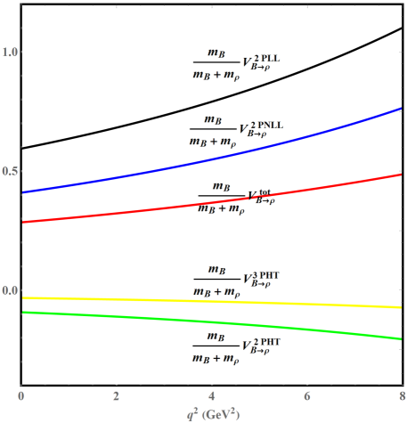
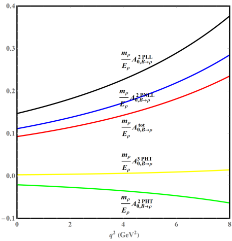
Figure 7: Breakdown of the various terms contributing to the two $B\to\rho$ form factors $V_{B\to\rho}(q^{2})$ and $A_{0,\,B\to\rho}(q^{2})$ from the SCET sum rules with the exponential model of the $B$-meson distribution amplitudes at $q^{2}\leq 8\,{\rm GeV^{2}}$. The individual contributions correspond to the two-particle leading-twist effects at LL (black curves) and at NLL (blue curves), the two-particle higher-twist corrections (green curves) and the three-particle higher-twist effects (yellow curves).

To develop a transparent understanding of the higher-order perturbative corrections and the higher-twist contributions from the two-particle and three-particle $B$-meson distribution amplitudes computed in this work, we display in figure 7 the numerical effects of distinct pieces contributing to the final sum rules for the two $B\to\rho$ form factors $V_{B\to\rho}(q^{2})$ and $A_{0,\,B\to\rho}(q^{2})$ at large hadronic recoil. It is evident that the NLL QCD radiative corrections to the leading-twist contributions can give rise to approximately $(25-30)\,\%$ reduction of the corresponding resummation improved tree-level predictions. In particular, the two-particle twist-five contributions to both the two $B\to\rho$ form factors at LO in QCD generate sizeable corrections, numerically $(20-30)\,\%$, to the leading-power predictions at NLL, in analogy to the earlier observation for $B\to\pi,K$ form factors [22] (see also [80] for independent calculations of the higher-twist effects up to the twist-four $B$-meson distribution amplitudes). By contrast, the genuine three-particle higher-twist corrections yield approximately ${\cal O}(10\,\%)$ and ${\cal O}(2\,\%)$ enhancement of the leading-twist calculations for the transverse and longitudinal $B\to\rho$ form factors, respectively. We have verified that the preceding observed patterns for the higher-order and higher-twist corrections are also satisfied for the SCET sum rules predictions of the remaining $B\to V$ (with $V=\rho,\omega,K^{\ast}$) form factors.

Now we proceed to investigate an interesting issue of QCD computations for the heavy-to-light $B$-meson decay form factors at large recoil from the SCET factorization approach and the LCSR method with the light-meson distribution amplitudes. Generally theory predictions for the form-factor ratios from these two different approaches are in reasonable agreement with each other, however, the obtained results for the following $B\to V$ form-factor ratios

$$\mathcal{R}_{1}={m_{B}+m_{V}\over m_{B}}\,{T_{1}\over V},\qquad\mathcal{R}_{2}={m_{B}/(2\,E)\,T_{2}-T_{3}\over(m_{B}+m_{V})/(2\,E)\,A_{1}-(m_{B}-m_{V})/m_{B}\,A_{2}}\,,$$ (192)

differ in both the magnitude and sign of the large-recoil symmetry breaking effects [4, 42, 62]. It is our purpose to address whether such discrepancies are due to the yet higher-order corrections in both $\alpha_{s}$ and $\Lambda/m_{b}$ or due to the systematic uncertainties of the method of QCD sum rules. To achieve this goal, we display our predictions for the form-factor ratios from the improved SCET sum rules with the $B$-meson distribution amplitudes in figure 8, including the corresponding NLL results from the QCD factorization approach for a comparison. It can be observed that our predictions for all the $B\to\rho$ form-factor ratios, particularly the sign of the symmetry breaking, are in agreement with the SCET results displayed in figure 6 of [42]. We are therefore led to conclude that the above-mentioned discrepancies between the two different QCD calculations mainly arise from the parton-hadron duality approximation for the $B$-meson channel implemented in the construction of the sum rules for the heavy-to-light form factors with the vector-meson distribution amplitudes. This can be also understood from the fact that the traditional LCSR for the semileptonic $B\to V$ form factors in the heavy-quark limit will introduce new non-perturbative quantities, for instance $\phi_{\perp}^{\prime}(1)$ and $\Phi_{\|}^{\prime}(1)$ [8], which cannot be constructed from a finite number of Gegenbauer moments of the corresponding vector-meson distribution amplitudes and whose field-theoretical definitions are absent in SCET [81]. On the contrary, the new LCSR for the ${\rm A0}$- and ${\rm B1}$- type SCET form factors with the $B$-meson distribution amplitudes involve the two quantities $\phi_{B}^{-}(0,\mu)$ and $\lambda_{B}^{-1}(\mu)$, which are identical in the Wandzura-Wilczek approximation (namely, neglecting the effect of the three-particle $B$-meson LCDA $\Psi_{A}-\Psi_{V}$) [82] and are well defined parameters in the SCET framework.

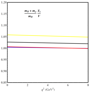
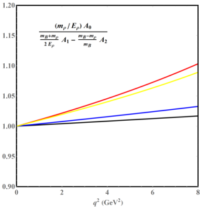
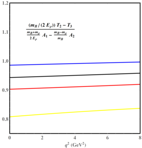
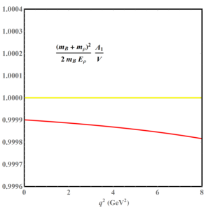
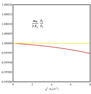
Figure 8: Theory predictions for the $B\to V$ form-factor ratios from the improved SCET sum rules derived in this work and from the QCD factorization approach with the so-called physical form factor scheme [4, 42]. Black curves: the leading-power contributions at the LL accuracy; blue curves: the leading-power contributions at the NLL accuracy; red curves: full results including both the leading-power effects at NLL and the subleading-twist corrections at LO up to the twist-six accuracy. The yellow curves are obtained from the leading-power computations with the QCD factorization approach at NLO.

In addition, we notice that the magnitudes of the large-recoil symmetry violations predicted from the SCET sum rules with $B$-meson distribution amplitudes are generally smaller than those predicted by the QCD factorization approach (see also [42] for a similar observation). To identify the underlying mechanism responsible for such discrepancy, we write down explicitly the separate terms generating the symmetry correction to $\mathcal{R}_{1}$

$$\mathcal{R}_{1,\,{\rm LCSR}} = 1+{[(-0.179)-(-0.154)]\times 0.560\over 0.285}\bigg{|}_{C_{i}^{(\rm A0)}}+{[(-1)+0.203]\times(-0.0192)\over 0.285}\bigg{|}_{C_{i}^{(\rm B1)}}$$

$$+{[(-0.0922)-(-0.0922)]\over 0.285}\bigg{|}_{\rm 2PHT}+{[(-0.03220)-(-0.03219)]\over 0.285}\bigg{|}_{\rm 3PHT}$$

$$= 1+(-0.049)\big{|}_{C_{i}^{(\rm A0)}}+(+0.054)\big{|}_{C_{i}^{(\rm B1)}}+(-3.5\times 10^{-5})\big{|}_{\rm 3PHT}\,,$$

$$\mathcal{R}_{1,\,{\rm QCDF}} = 1+(-0.023)\big{|}_{C_{i}^{(\rm A0)}}+(+0.086)\,[1+{\cal O}(\alpha_{s})]\big{|}_{C_{i}^{(\rm B1)}}\,,$$ (193)

where the expression of $\mathcal{R}_{1,\,{\rm QCDF}}$ is borrowed directly from (124) of [42] by dropping out the NLO correction to the hard-spectator scattering contribution. It is then evident that the negligible symmetry breaking effect from the $B$-meson LCSR calculation is due to the strong cancellation between the ${\rm A0}$- and ${\rm B1}$-type SCET matrix elements weighted by the corresponding hard matching coefficients. By contrast, the symmetry violation predicted in QCD factorization is numerically dominated by the hard-spectator scattering and will be further enhanced by the higher-order perturbative correction and the RG resummation effect as indicated in [42]. More specifically, the strong cancellation mechanics from the $B$-meson LCSR computation can be attributed to the following reasoning.

• The LCSR prediction of the non-local SCET form factor $\Xi_{\perp}(\tau,n\cdot p)$ is approximately $40\%$ smaller than the QCD factorization result at tree level. This observation implies that approximating the collinear dynamics of the energetic vector meson by the static QCD decay constants is numerically insufficient for the theory description of the semileptonic $B\to V$ form factors beyond the heavy quark limit.

• At the one-loop accuracy, the NLO corrections to the hard functions of the ${\rm A0}$-type SCET operators must be multiplied with the LO sum rule result of the ${\rm A0}$-type form factor $\xi_{\perp}(n\cdot p)$ instead of the physics QCD form factor

  $$\xi_{\perp}^{\rm FF}(n\cdot p)\equiv{m_{B}\over m_{B}+m_{V}}\,V(n\cdot p)\,,$$ (194)

  which has to be taken as an hadronic input in QCD factorization. The SCET sum rule prediction of $\xi_{\perp}(m_{B})$ with $B$-meson distribution amplitudes at tree level is approximately twice of the complete result for $\xi_{\perp}^{\rm FF}(m_{B})$ including both the NLO QCD correction and the higher-twist correction. As a consequence, our prediction for the symmetry correction due to $C_{i,\,\rm{NLL}}^{(\rm A0)}\,\,\xi_{\perp}$ is enhanced by a factor of two when compared with the corresponding QCD factorization computation.

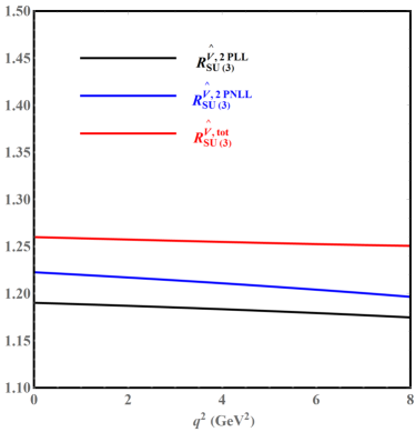
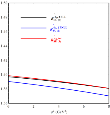
Figure 9: The SU(3) symmetry breaking effects for the transverse form factor ${m_{B}\over m_{B}+m_{V}}\,V(q^{2})$ and for the longitudinal form factor ${m_{V}\over E_{V}}\,A_{0}(q^{2})$ at large hadronic recoil, computed from the SCET sum rules with $B$-meson distribution amplitudes.

We now explore the SU(3) flavour symmetry breaking effects between $B\to\rho$ and $B\to K^{\ast}$ form factors from the $B$-meson LCSR numerically. In our theoretical framework they originate from the explicit corrections proportional to the light-quark masses and the light vector meson masses, the differences in the values of the threshold parameters and Boreal masses, and the discrepancies in the longitudinal and transverse decay constants for $\rho$ and $K^{\ast}$. Additional sources of the SU(3) flavour symmetry violations due to the electromagnetic corrections and the process-dependent systematic uncertainties (e.g., the parton-hadron duality ansatz) are not taken into account. For the phenomenological convenience we introduce the following quantity to character the SU(3) symmetry corrections

$$R_{\rm SU(3)}^{i}(q^{2})={F_{B\to K^{\ast}}^{i}(q^{2})\over F_{B\to\rho}^{i}(q^{2})}\,,$$ (195)

where $F_{B\to V}^{i}$ represent the seven QCD form-factor combinations appearing in (8) generally. It is evident from figure 9 the SU(3) flavour symmetry breaking effects for the transverse and longitudinal $B\to V$ form factors are approximately $25\%$ and $40\%$ in the large recoil region $0\,{\rm GeV^{2}}\leq q^{2}\leq 8\,{\rm GeV^{2}}$, respectively. This pattern can be understood from the fact that the leading-power light-quark mass effect does not contribute to the SCET form factor $\xi_{\perp}(n\cdot p)$ at the one-loop approximation as demonstrated in (103). Our predictions for the SU(3) flavour symmetry corrections are in excellent agreement with the previous computations based upon the LCSR method with the vector-meson distribution amplitudes [10], but are significantly larger than the updated results presented in [11], which predicted remarkably small flavour symmetry violations (approximately $2\,\%$ and $15\,\%$ for the transverse and longitudinal $B\to V$ form factors at the maximal hadronic recoil). We further notice that the subleading power higher-twist corrections are of minor numerical importance for generating the SU(3) flavour symmetry breaking effects.

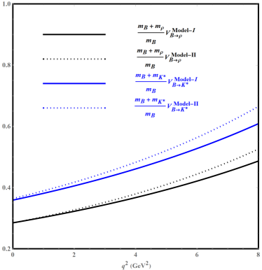
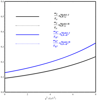
Figure 10: Model dependence of the transverse and longitudinal $B\to\rho,\,K^{\ast}$ form factors on the shapes of $B$-meson distribution amplitudes at $0\leq q^{2}\leq 8\,{\rm GeV^{2}}$. The superscripts “Model-I” and “Model-II” refer to the exponential model and the local duality model of the two-particle and three-particle $B$-meson LCDA displayed in Appendix B.

As already demonstrated in [20], the knowledge of the complete functional forms of the $B$-meson distribution amplitudes is in demand for the evaluation for the heavy-to-light $B$-meson decay form factors. To reduce the model dependence of our predictions, the inverse moment $\lambda_{B}(\mu_{0})$ for a given model of the $B$-meson LCDA has been determined by reproducing the alternative LCSR prediction for $V_{B\to\rho}(q^{2}=0)$ with the vector-meson LCDA as described in the previous paragraphs. In other words, we aim at predicting the momentum-transfer dependence of the transverse $B\to\rho$ form factor $V_{B\to\rho}(q^{2})$ merely. However, both the normalization factors at the maximal recoil and the $q^{2}$-shapes for all the remaining form factors will be obtained from the derived SCET sum rules subsequently. It can be observed from figure 10 that the model dependence of our predictions on the precise $\omega$-behaviours of the $B$-meson distribution amplitudes is drastically reduced by implementing the above-mentioned prescription, in analogy to the earlier observation for the semileptonic $B\to\pi,K$ form factors computed in the same framework [20, 22].

Evidently, the obtained LCSR for the SCET form factors $\xi_{i}(n\cdot p)$ and $\Xi_{i}(\tau,n\cdot p)$ (with $i=\|,\,\perp$) cannot be constructed without demonstrating the soft-collinear factorization for the various vacuum-to-$B$-meson correlation functions under discussion in the first place, which can be validated with the light-cone operator product expansion (OPE) technique only at the large hadronic recoil. To extrapolate the SCET sum rule predictions for the $B\to V$ form factors toward the high $q^{2}$ region, we will employ the model-independent $z$-series parametrizations [83] motivated by the analytical properties and the asymptotic behaviours of the heavy-to-light form factors. The complex cut $q^{2}$-plane will then be mapped onto the unit disc $z(q^{2},t_{0})\leq 1$ under the conformal transformation

$$z(q^{2},t_{0})=\frac{\sqrt{t_{+}-q^{2}}-\sqrt{t_{+}-t_{0}}}{\sqrt{t_{+}-q^{2}}+\sqrt{t_{+}-t_{0}}}\,,$$ (196)

where two parameters $t_{+}$ and $t_{0}$ are given by [22] (see also [84])

$$t_{+}=(m_{B}+m_{V})^{2}\,,\qquad t_{0}=(m_{B}-m_{V})^{2}\,.$$ (197)

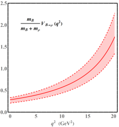
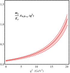
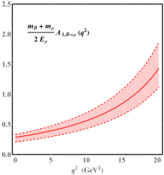
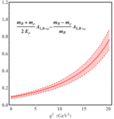
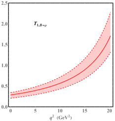
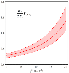
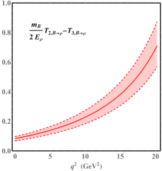
Figure 11: Theory predictions of the semileptonic $B\to\rho$ form factors obtained from the SCET sum rules with the $B$-meson distribution amplitudes with an extrapolation to the entire kinematical region by applying the $z$-series parametrizations (198).

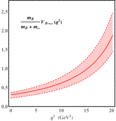
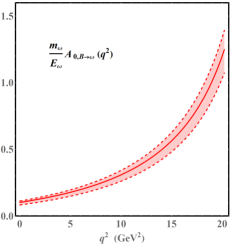
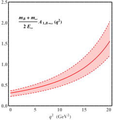
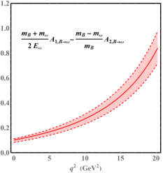
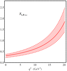
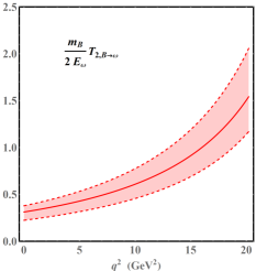
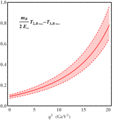
Figure 12: Theory predictions of the semileptonic $B\to\omega$ form factors obtained from the SCET sum rules with the $B$-meson distribution amplitudes with an extrapolation to the entire kinematical region by applying the $z$-series parametrizations (198).

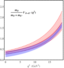
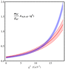
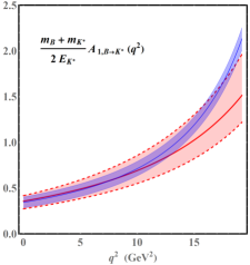
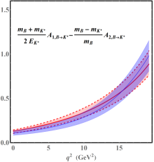
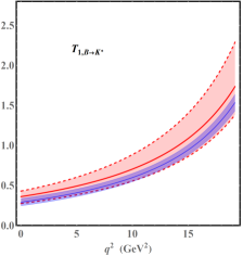
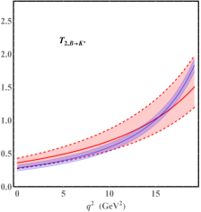
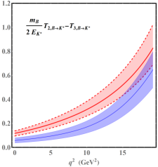
Figure 13: Theory predictions of the electro-weak penguin $B\to K^{\ast}$ decay form factors obtained from the SCET sum rules with the $B$-meson distribution amplitudes with an extrapolation to the entire kinematical region by applying the $z$-series parametrizations (198). We also display the Lattice QCD predictions for these form factors with $2+1$ flavours of sea quarks [1, 2] as indicated by the blue bands for a comparison.

For the phenomenological applications we will adopt the Bourrely-Caprini-Lellouch (BCL) version of the $z$-series expansion [85] (see [86] for an alternative version and [87] for more discussions in the context of the semileptonic $B\to\pi$ form factors)

$$F_{B\to V}^{i}(q^{2})={F_{B\to V}^{i}(0)\over 1-q^{2}/m_{i,\,\rm pole}^{2}}\,\left\{1+\sum_{k=1}^{N}\,b_{k}^{i}\,\left[z(q^{2},t_{0})^{k}-z(0,t_{0})^{k}\right]\right\}\,.$$ (198)

The adopted values of the various resonance masses from the Particle Data Group (PDG) [77] and from the heavy-hadron chiral perturbation theory [88] are summarized in Table 1.

$F_{B\to V}^{i}(q^{2})$	$J^{P}$	$b\to d$   (in ${\rm GeV}$)	$b\to s$   (in ${\rm GeV}$)
$\mathcal{V}(q^{2})$,   $\mathcal{T}_{1}(q^{2})$	$1^{-}$	5.325	5.415
$\mathcal{A}_{0}(q^{2})$	$0^{-}$	5.279	5.366
$\mathcal{A}_{1}(q^{2})$,   $\mathcal{A}_{12}(q^{2})$,   $\mathcal{T}_{2}(q^{2})$   $\mathcal{T}_{23}(q^{2})$	$1^{+}$	5.724	5.829

Table 1: Theory summary of the resonance masses with different quantum numbers entering the $z$-series expansions of the QCD $B\to V$ form factors (198). The calligraphic form factors represent the linear combinations of the conventionally defined form factors, appearing in the ${\rm SCET_{I}}$ factorization formulae (8) directly.

For the practical purpose we will truncate the $z$-series expansion (198) at $N=1$ for the sake of fitting the coefficients $b_{k}^{i}$, keeping in mind that $|z(q^{2},t_{0})|^{2}\leq 0.04$ in the whole kinematic region (see [89] for further discussions on the systematic uncertainties due to the truncation-scheme dependence and [90] on the implementation of the strong unitary constraints).

It is straightforward to implement the matching procedure for the semileptonic $B\to V$ form factors by employing the improved LCSR calculations at $-6\,{\rm GeV}^{2}\leq q^{2}\leq 8\,{\rm GeV}^{2}$ and the $z$-series parametrizations (198). Our predictions for the twenty-one form factors responsible for the exclusive $B\to\rho,\,\omega,\,K^{\ast}$ transitions in the entire kinematic region are displayed in figures 11, 12 and 13, where the theory uncertainties are obtained by adding all the separate uncertainties in quadrature and the updated Lattice QCD results of $B\to\,K^{\ast}$ form factors with physical-mass bottom quarks and $2+1$ flavours of sea quarks [2] are also shown for a comparison. Generally these two different QCD techniques lead to consistent form-factor predictions at large hadronic recoil, with the exception of the longitudinal form factor $m_{B}/(2\,E_{K^{\ast}})\,T_{2,\,B\to K^{\ast}}(q^{2})-T_{3,\,B\to K^{\ast}}(q^{2})$. Such discrepancy may be attributed to the fact that the form factor $T_{3}(q^{2})$ cannot be isolated directly from the helicity form factor $T_{23}(q^{2})$ at large $q^{2}$ in the Lattice QCD simulations [1], due to the phase-space suppression. We further collect the fitted results for the shape parameters $b_{k}^{i}$ and the normalization constants $F_{B\to V}^{i}(0)$ entering the $z$-expansion (198) with numerically important uncertainties in Tables 2, 3, 4, 5, 6, 7. Several remarks on the obtained numerical results are in order.

• It is evident that the dominant theory uncertainties of the resulting predictions for $F_{B\to V}^{i}(0)$ and $b_{k}^{i}$ originate from the model dependence of the $B$-meson distribution amplitudes at a reference scale (including the (logarithmic)-inverse moments $\lambda_{B}$ and $\sigma_{1}$), the factorization scale $\mu$ and the QCD renormalization scale $\nu$ for the tensor weak transition currents. Consequently, it is of interest to perform the non-perturbative determination of the momentum-dependence of the leading-twist $B$-meson LCDA with the Lattice QCD technique and to compute the yet higher-order perturbative QCD corrections to the ${\rm A0}$- and ${\rm B}$-type SCET form factors with the method of sum rules.

• Our theory predictions for the QCD $B\to\rho,\,\,K^{\ast}$ form factors in the whole kinematic region are in reasonable agreement with the previous calculations applying the same framework [80]. However, the leading-twist contributions to $B\to M$ form factors were only computed at LO in the strong coupling $\alpha_{s}$ [80] without implementing the summation of enhanced logarithms of $m_{b}/\Lambda$. In addition, the higher-twist corrections from the three-particle $B$-meson distribution amplitudes were also estimated at the twist-four accuracy [80], implying the violation of the QCD equation of motion (152) already at the classical level. It needs further to be pointed out that a comprehensive study of the higher-twist $B$-meson LCDA up to the twist-six accuracy, including both the off light-cone corrections and the four-body light-ray HQET operator effects, still remains as an interesting problem for the future improvement.

Parameters	Central    value	$\lambda_{B}$	$\sigma_{1}$	$\mu$	$\nu$	$M^{2}$	$s_{0}$	$\phi_{B}^{\pm}(\omega)$
$\mathcal{V}_{B\rightarrow\rho}\text{(0)}$	$0.285$	${}_{-0.027}^{+0.027}$	${}_{-0.016}^{+0.016}$	${}_{-0.055}^{+0.002}$	-	${}_{-0.000}^{+0.001}$	${}_{-0.018}^{+0.016}$	${}_{-0.027}^{+0.028}$
$b_{1,\rho}^{\mathcal{V}}$	$-3.72$	${}_{-0.09}^{+0.14}$	${}_{-0.06}^{+0.08}$	${}_{-0.76}^{+0.45}$	-	${}_{-0.07}^{+0.03}$	${}_{-0.09}^{+0.08}$	${}_{-1.43}^{+0.00}$
$\mathcal{A}_{0,B\rightarrow\rho}\text{(0)}$	$0.093$	${}_{-0.006}^{+0.006}$	${}_{-0.004}^{+0.004}$	${}_{-0.011}^{+0.000}$	-	${}_{-0.000}^{+0.000}$	${}_{-0.003}^{+0.002}$	${}_{-0.010}^{+0.004}$
$b_{1,\rho}^{\mathcal{A}_{0}}$	$-11.9$	${}_{-0.1}^{+0.1}$	${}_{-0.1}^{+0.1}$	${}_{-0.6}^{+0.2}$	-	${}_{-0.4}^{+0.2}$	${}_{-0.1}^{+0.1}$	${}_{-0.9}^{+0.0}$
$\mathcal{A}_{1,B\rightarrow\rho}\text{(0)}$	$0.285$	${}_{-0.027}^{+0.027}$	${}_{-0.016}^{+0.016}$	${}_{-0.055}^{+0.002}$	-	${}_{-0.001}^{+0.001}$	${}_{-0.018}^{+0.016}$	${}_{-0.027}^{+0.028}$
$b_{1,\rho}^{\mathcal{A}_{1}}$	$-4.63$	${}_{-0.10}^{+0.15}$	${}_{-0.06}^{+0.08}$	${}_{-0.78}^{+0.46}$	-	${}_{-0.07}^{+0.03}$	${}_{-0.09}^{+0.08}$	${}_{-1.48}^{+0.00}$
$\mathcal{A}_{12,B\rightarrow\rho}\text{(0)}$	$0.093$	${}_{-0.006}^{+0.006}$	${}_{-0.004}^{+0.004}$	${}_{-0.011}^{+0.000}$	-	${}_{-0.000}^{+0.000}$	${}_{-0.003}^{+0.002}$	${}_{-0.010}^{+0.004}$
$b_{1,\rho}^{\mathcal{A}_{12}}$	$-10.8$	${}_{-0.0}^{+0.1}$	${}_{-0.0}^{+0.0}$	${}_{-0.5}^{+0.3}$	-	${}_{-0.2}^{+0.1}$	${}_{-0.1}^{+0.1}$	${}_{-1.4}^{+0.0}$

Table 2: Theory summary of the fitted results for the shape parameters and normalizations of the (axial)-vector $B\to\rho$ form factors with the numerically sizeable uncertainties by varying different input parameters.

Parameters	Central    value	$\lambda_{B}$	$\sigma_{1}$	$\mu$	$\nu$	$M^{2}$	$s_{0}$	$\phi_{B}^{\pm}(\omega)$
$\mathcal{T}_{1,B\rightarrow\rho}\text{(0)}$	$0.287$	${}_{-0.027}^{+0.027}$	${}_{-0.016}^{+0.016}$	${}_{-0.055}^{+0.002}$	${}_{-0.016}^{+0.026}$	${}_{-0.000}^{+0.001}$	${}_{-0.018}^{+0.016}$	${}_{-0.027}^{+0.028}$
$b_{1,\rho}^{\mathcal{T}_{1}}$	$-3.57$	${}_{-0.10}^{+0.15}$	${}_{-0.06}^{+0.08}$	${}_{-0.73}^{+0.44}$	${}_{-0.07}^{+0.04}$	${}_{-0.06}^{+0.03}$	${}_{-0.08}^{+0.08}$	${}_{-1.43}^{+0.00}$
$\mathcal{T}_{2,B\rightarrow\rho}\text{(0)}$	$0.287$	${}_{-0.027}^{+0.027}$	${}_{-0.016}^{+0.016}$	${}_{-0.055}^{+0.002}$	${}_{-0.016}^{+0.026}$	${}_{-0.000}^{+0.001}$	${}_{-0.018}^{+0.016}$	${}_{-0.027}^{+0.028}$
$b_{1,\rho}^{\mathcal{T}_{2}}$	$-4.48$	${}_{-0.10}^{+0.16}$	${}_{-0.07}^{+0.08}$	${}_{-0.75}^{+0.46}$	${}_{-0.07}^{+0.04}$	${}_{-0.06}^{+0.03}$	${}_{-0.09}^{+0.08}$	${}_{-1.47}^{+0.00}$
$\mathcal{T}_{23,B\rightarrow\rho}\text{(0)}$	$0.084$	${}_{-0.006}^{+0.006}$	${}_{-0.004}^{+0.004}$	${}_{-0.011}^{+0.000}$	${}_{-0.004}^{+0.007}$	${}_{-0.000}^{+0.001}$	${}_{-0.003}^{+0.002}$	${}_{-0.006}^{+0.007}$
$b_{1,\rho}^{\mathcal{T}_{23}}$	$-11.3$	${}_{-0.0}^{+0.1}$	${}_{-0.0}^{+0.0}$	${}_{-0.6}^{+0.4}$	${}_{-0.1}^{+0.0}$	${}_{-0.2}^{+0.1}$	${}_{-0.1}^{+0.1}$	${}_{-1.5}^{+0.0}$

Table 3: Theory summary of the fitted results for the shape parameters and normalizations of the tensor $B\to\rho$ form factors with the numerically sizeable uncertainties by varying different input parameters.

Parameters	Central    value	$\lambda_{B}$	$\sigma_{1}$	$\mu$	$\nu$	$M^{2}$	$s_{0}$	$\phi_{B}^{\pm}(\omega)$
$\mathcal{V}_{B\rightarrow\omega}\text{(0)}$	$0.311$	${}_{-0.030}^{+0.030}$	${}_{-0.018}^{+0.017}$	${}_{-0.060}^{+0.002}$	-	${}_{-0.000}^{+0.001}$	${}_{-0.019}^{+0.018}$	${}_{-0.030}^{+0.030}$
$b_{1,\omega}^{\mathcal{V}}$	$-3.73$	${}_{-0.09}^{+0.14}$	${}_{-0.06}^{+0.08}$	${}_{-0.76}^{+0.45}$	-	${}_{-0.07}^{+0.04}$	${}_{-0.09}^{+0.08}$	${}_{-1.44}^{+0.00}$
$\mathcal{A}_{0,B\rightarrow\omega}\text{(0)}$	$0.102$	${}_{-0.007}^{+0.007}$	${}_{-0.004}^{+0.004}$	${}_{-0.012}^{+0.000}$	-	${}_{-0.000}^{+0.001}$	${}_{-0.003}^{+0.003}$	${}_{-0.011}^{+0.004}$
$b_{1,\omega}^{\mathcal{A}_{0}}$	$-11.9$	${}_{-0.1}^{+0.1}$	${}_{-0.1}^{+0.1}$	${}_{-0.6}^{+0.2}$	-	${}_{-0.4}^{+0.2}$	${}_{-0.1}^{+0.1}$	${}_{-0.9}^{+0.0}$
$\mathcal{A}_{1,B\rightarrow\omega}\text{(0)}$	$0.310$	${}_{-0.030}^{+0.030}$	${}_{-0.018}^{+0.017}$	${}_{-0.060}^{+0.002}$	-	${}_{-0.000}^{+0.001}$	${}_{-0.019}^{+0.018}$	${}_{-0.030}^{+0.030}$
$b_{1,\omega}^{\mathcal{A}_{1}}$	$-4.64$	${}_{-0.10}^{+0.15}$	${}_{-0.06}^{+0.08}$	${}_{-0.78}^{+0.46}$	-	${}_{-0.07}^{+0.04}$	${}_{-0.09}^{+0.08}$	${}_{-1.48}^{+0.00}$
$\mathcal{A}_{12,B\rightarrow\omega}\text{(0)}$	$0.102$	${}_{-0.007}^{+0.007}$	${}_{-0.004}^{+0.004}$	${}_{-0.012}^{+0.000}$	-	${}_{-0.000}^{+0.001}$	${}_{-0.003}^{+0.003}$	${}_{-0.011}^{+0.004}$
$b_{1,\omega}^{\mathcal{A}_{12}}$	$-10.9$	${}_{-0.0}^{+0.1}$	${}_{-0.0}^{+0.0}$	${}_{-0.5}^{+0.3}$	-	${}_{-0.2}^{+0.1}$	${}_{-0.1}^{+0.1}$	${}_{-1.4}^{+0.0}$

Table 4: Theory summary of the fitted results for the shape parameters and normalizations of the (axial)-vector $B\to\omega$ form factors with the numerically sizeable uncertainties by varying different input parameters.

Parameters	Central    value	$\lambda_{B}$	$\sigma_{1}$	$\mu$	$\nu$	$M^{2}$	$s_{0}$	$\phi_{B}^{\pm}(\omega)$
$\mathcal{T}_{1,B\rightarrow\omega}\text{(0)}$	$0.312$	${}_{-0.030}^{+0.030}$	${}_{-0.018}^{+0.018}$	${}_{-0.061}^{+0.002}$	${}_{-0.017}^{+0.028}$	${}_{-0.000}^{+0.001}$	${}_{-0.020}^{+0.018}$	${}_{-0.029}^{+0.031}$
$b_{1,\omega}^{\mathcal{T}_{1}}$	$-3.58$	${}_{-0.10}^{+0.15}$	${}_{-0.06}^{+0.08}$	${}_{-0.73}^{+0.44}$	${}_{-0.07}^{+0.04}$	${}_{-0.06}^{+0.03}$	${}_{-0.08}^{+0.08}$	${}_{-1.43}^{+0.00}$
$\mathcal{T}_{2,B\rightarrow\omega}\text{(0)}$	$0.312$	${}_{-0.030}^{+0.030}$	${}_{-0.018}^{+0.018}$	${}_{-0.061}^{+0.002}$	${}_{-0.017}^{+0.028}$	${}_{-0.000}^{+0.001}$	${}_{-0.020}^{+0.018}$	${}_{-0.029}^{+0.031}$
$b_{1,\omega}^{\mathcal{T}_{2}}$	$-4.49$	${}_{-0.10}^{+0.16}$	${}_{-0.06}^{+0.08}$	${}_{-0.75}^{+0.46}$	${}_{-0.07}^{+0.04}$	${}_{-0.06}^{+0.03}$	${}_{-0.09}^{+0.08}$	${}_{-1.47}^{+0.00}$
$\mathcal{T}_{23,B\rightarrow\omega}\text{(0)}$	$0.092$	${}_{-0.007}^{+0.007}$	${}_{-0.004}^{+0.004}$	${}_{-0.012}^{+0.000}$	${}_{-0.005}^{+0.008}$	${}_{-0.000}^{+0.000}$	${}_{-0.003}^{+0.003}$	${}_{-0.007}^{+0.008}$
$b_{1,\omega}^{\mathcal{T}_{23}}$	$-11.3$	${}_{-0.0}^{+0.1}$	${}_{-0.0}^{+0.0}$	${}_{-0.7}^{+0.4}$	${}_{-0.1}^{+0.0}$	${}_{-0.2}^{+0.1}$	${}_{-0.1}^{+0.1}$	${}_{-1.5}^{+0.0}$

Table 5: Theory summary of the fitted results for the shape parameters and normalizations of the tensor $B\to\omega$ form factors with the numerically sizeable uncertainties by varying different input parameters.

Parameters	Central    value	$\lambda_{B}$	$\sigma_{1}$	$\mu$	$\nu$	$M^{2}$	$s_{0}$	$\phi_{B}^{\pm}(\omega)$
$\mathcal{V}_{B\rightarrow K^{*}}\text{(0)}$	$0.359$	${}_{-0.032}^{+0.032}$	${}_{-0.019}^{+0.019}$	${}_{-0.062}^{+0.001}$	-	${}_{-0.004}^{+0.010}$	${}_{-0.017}^{+0.016}$	${}_{-0.027}^{+0.038}$
$b_{1,K^{*}}^{\mathcal{V}}$	$-3.94$	${}_{-0.06}^{+0.11}$	${}_{-0.04}^{+0.06}$	${}_{-0.73}^{+0.42}$	-	${}_{-0.07}^{+0.04}$	${}_{-0.08}^{+0.08}$	${}_{-1.41}^{+0.00}$
$\mathcal{A}_{0,B\rightarrow K^{*}}\text{(0)}$	$0.129$	${}_{-0.008}^{+0.008}$	${}_{-0.005}^{+0.005}$	${}_{-0.016}^{+0.001}$	-	${}_{-0.002}^{+0.004}$	${}_{-0.003}^{+0.003}$	${}_{-0.011}^{+0.006}$
$b_{1,K^{*}}^{\mathcal{A}_{0}}$	$-12.4$	${}_{-0.1}^{+0.1}$	${}_{-0.1}^{+0.1}$	${}_{-0.6}^{+0.2}$	-	${}_{-0.3}^{+0.2}$	${}_{-0.1}^{+0.1}$	${}_{-0.9}^{+0.0}$
$\mathcal{A}_{1,B\rightarrow K^{*}}\text{(0)}$	$0.358$	${}_{-0.032}^{+0.031}$	${}_{-0.019}^{+0.018}$	${}_{-0.062}^{+0.001}$	-	${}_{-0.005}^{+0.010}$	${}_{-0.017}^{+0.016}$	${}_{-0.026}^{+0.039}$
$b_{1,K^{*}}^{\mathcal{A}_{1}}$	$-4.81$	${}_{-0.07}^{+0.12}$	${}_{-0.05}^{+0.06}$	${}_{-0.75}^{+0.43}$	-	${}_{-0.07}^{+0.04}$	${}_{-0.08}^{+0.08}$	${}_{-1.48}^{+0.00}$
$\mathcal{A}_{12,B\rightarrow K^{*}}\text{(0)}$	$0.129$	${}_{-0.008}^{+0.008}$	${}_{-0.005}^{+0.005}$	${}_{-0.016}^{+0.001}$	-	${}_{-0.002}^{+0.004}$	${}_{-0.003}^{+0.003}$	${}_{-0.011}^{+0.006}$
$b_{1,K^{*}}^{\mathcal{A}_{12}}$	$-11.3$	${}_{-0.0}^{+0.1}$	${}_{-0.0}^{+0.0}$	${}_{-0.5}^{+0.3}$	-	${}_{-0.2}^{+0.1}$	${}_{-0.1}^{+0.1}$	${}_{-1.5}^{+0.0}$

Table 6: Theory summary of the fitted results for the shape parameters and normalizations of the (axial)-vector $B\to K^{\ast}$ form factors with the numerically sizeable uncertainties by varying different input parameters.

Parameters	Central    value	$\lambda_{B}$	$\sigma_{1}$	$\mu$	$\nu$	$M^{2}$	$s_{0}$	$\phi_{B}^{\pm}(\omega)$
$\mathcal{T}_{1,B\rightarrow K^{*}}\text{(0)}$	$0.361$	${}_{-0.032}^{+0.032}$	${}_{-0.019}^{+0.019}$	${}_{-0.062}^{+0.001}$	${}_{-0.019}^{+0.032}$	${}_{-0.004}^{+0.011}$	${}_{-0.017}^{+0.016}$	${}_{-0.026}^{+0.039}$
$b_{1,K^{*}}^{\mathcal{T}_{1}}$	$-3.78$	${}_{-0.07}^{+0.11}$	${}_{-0.05}^{+0.06}$	${}_{-0.71}^{+0.41}$	${}_{-0.06}^{+0.04}$	${}_{-0.07}^{+0.04}$	${}_{-0.08}^{+0.07}$	${}_{-1.41}^{+0.00}$
$\mathcal{T}_{2,B\rightarrow K^{*}}\text{(0)}$	$0.361$	${}_{-0.032}^{+0.032}$	${}_{-0.019}^{+0.019}$	${}_{-0.062}^{+0.001}$	${}_{-0.019}^{+0.032}$	${}_{-0.004}^{+0.011}$	${}_{-0.017}^{+0.016}$	${}_{-0.026}^{+0.039}$
$b_{1,K^{*}}^{\mathcal{T}_{2}}$	$-4.67$	${}_{-0.07}^{+0.12}$	${}_{-0.05}^{+0.07}$	${}_{-0.72}^{+0.42}$	${}_{-0.07}^{+0.04}$	${}_{-0.07}^{+0.04}$	${}_{-0.08}^{+0.08}$	${}_{-1.46}^{+0.00}$
$\mathcal{T}_{23,B\rightarrow K^{*}}\text{(0)}$	$0.117$	${}_{-0.008}^{+0.008}$	${}_{-0.005}^{+0.005}$	${}_{-0.016}^{+0.000}$	${}_{-0.006}^{+0.010}$	${}_{-0.001}^{+0.003}$	${}_{-0.003}^{+0.003}$	${}_{-0.006}^{+0.011}$
$b_{1,K^{*}}^{\mathcal{T}_{23}}$	$-11.8$	${}_{-0.0}^{+0.1}$	${}_{-0.0}^{+0.0}$	${}_{-0.7}^{+0.4}$	${}_{-0.1}^{+0.0}$	${}_{-0.2}^{+0.1}$	${}_{-0.1}^{+0.1}$	${}_{-1.5}^{+0.0}$

Table 7: Theory summary of the fitted results for the shape parameters and normalizations of the tensor $B\to K^{\ast}$ form factors with the numerically sizeable uncertainties by varying different input parameters.

5.3 Semileptonic $B\to(\rho,\omega)\,\ell\bar{\nu}_{\ell}$ decays

Having at our disposal the theory predictions for all the $B\to\rho,\,\omega$ form factors in QCD, we proceed to investigate the phenomenological aspects of the semileptonic $B\to(\rho,\omega)\,\ell\,\bar{\nu}_{\ell}$ decays, which provide a complementary way for the exclusive determination of the CKM matrix element $|V_{ub}|$. However, we will not explore the further applications of the calculated form factors to the more challenging radiative and electroweak penguin $B$-meson decays, which are crucial to the precision extraction of the CKM matrix element $|V_{td}|$ [91] and to the intensive hunting of new physics beyond the Standard Model (SM) [92, 18, 19], due to the appearance of the complex non-local hadronic matrix elements even at leading power in the heavy quark expansion. The differential decay rate of $B\to V\,\ell\,\bar{\nu}_{\ell}$ can be readily written as

$$\frac{d^{2}\Gamma(B\to V\,\ell\,\bar{\nu}_{\ell})}{dq^{2}\,d\cos\theta} = {G_{F}^{2}\,|V_{ub}|^{2}\over 256\,\pi^{3}\,m_{B}^{3}}\,{q^{2}\over c_{V}^{2}}\,\lambda^{1/2}(m_{B}^{2},m_{V}^{2},q^{2})\,\bigg{\{}\sin^{2}\theta\,\,|H_{0}(q^{2})|^{2}+(1-\cos\theta)^{2}\,{|H_{+}(q^{2})|^{2}\over 2}$$ (199)

$$+\,(1+\cos\theta)^{2}\,{|H_{-}(q^{2})|^{2}\over 2}\bigg{\}}\,,$$

where the three helicity amplitudes $H_{i}(q^{2})$ ($i=\pm,\,0$) can be expressed in terms of the semileptonic $B\to V$ form factors

$$H_{\pm}(q^{2}) = (m_{B}+m_{V})\,\left[A_{1}(q^{2})\mp{2\,m_{B}\,|\vec{p}_{V}|\over(m_{B}+m_{V})^{2}}\,V(q^{2})\right]\,,$$

$$H_{0}(q^{2}) = {m_{B}+m_{V}\over 2\,m_{V}\,\sqrt{q^{2}}}\,\bigg{[}(m_{B}^{2}-m_{V}^{2}-q^{2})\,A_{1}(q^{2})-{4\,m_{B}^{2}\,|\vec{p}_{V}|^{2}\over(m_{B}+m_{V})^{2}}\,A_{2}(q^{2})\bigg{]}\,,$$ (200)

with the momentum $|\vec{p}_{V}|$ of the light-vector meson in the $B$-meson rest frame given by

$$|\vec{p}_{V}|={1\over 2\,m_{B}}\,\lambda^{1/2}(m_{B}^{2},m_{V}^{2},q^{2})\,,\qquad\lambda(a,b,c)=a^{2}+b^{2}+c^{2}-2ab-2ac-2bc\,.$$ (201)

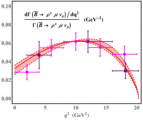
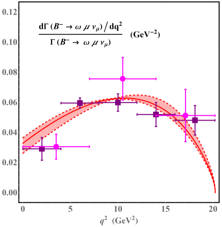
Figure 14: The normalized differential $q^{2}$ distributions of the semileptonic $B\to V\,\ell\,\bar{\nu}_{\ell}$ ($V=\rho,\,\omega$) decays with the heavy-to-light form factors computed in this work (red band). For a comparison, we also display the experimental measurements for the binned distributions from the BaBar [93, 95] and Belle [94] Collaborations.

For the determination of the CKM matrix element $|V_{ub}|$ we introduce the standard quantity

$$\Delta\zeta_{V}(q_{1}^{2},q_{2}^{2})={1\over|V_{ub}|^{2}}\,\int_{q_{1}^{2}}^{q_{2}^{2}}\,dq^{2}\,{d\Gamma(B\to V\,\ell\,\bar{\nu}_{\ell})\over dq^{2}}\,,$$ (202)

which can be computed by performing the phase-space integration over the obtained hadronic $B\to V$ form factors. The resulting predictions for $\Delta\zeta_{V}$ with the theoretical uncertainties from varying the input parameters are given by

$$\Delta\zeta_{\rho}(0,16\,{\rm GeV}^{2}) = \left(14.35\,{}^{+2.59}_{-2.41}\,\big{|}_{\lambda_{B}}\,{}^{+1.49}_{-1.46}\,\big{|}_{\sigma_{B}^{(1)}}\,{}^{+0.00}_{-3.63}\,\big{|}_{\mu}\,{}^{+0.29}_{-1.02}\,\big{|}_{\mu_{h1}}\,{}^{+0.71}_{-1.60}\,\big{|}_{\mu_{h2}}\,{}^{+1.14}_{-1.24}\,\big{|}_{s_{0}}\,{}^{+4.43}_{-1.16}\,\big{|}_{\phi_{B}^{\pm}}\right)\,\,\,{\rm ps}^{-1}$$

$$= 14.35^{+5.71}_{-5.41}\,\,\,{\rm ps}^{-1}\,,$$

$$\Delta\zeta_{\omega}(0,12\,{\rm GeV}^{2}) = \left(6.25\,{}^{+1.08}_{-1.01}\,\big{|}_{\lambda_{B}}\,{}^{+0.62}_{-0.61}\,\big{|}_{\sigma_{B}^{(1)}}\,{}^{+0.00}_{-1.59}\,\big{|}_{\mu}\,{}^{+0.11}_{-0.41}\,\big{|}_{\mu_{h1}}\,{}^{+0.28}_{-0.65}\,\big{|}_{\mu_{h2}}\,{}^{+0.48}_{-0.52}\,\big{|}_{s_{0}}\,{}^{+1.63}_{-0.66}\,\big{|}_{\phi_{B}^{\pm}}\right)\,\,\,{\rm ps}^{-1}$$ (203)

$$= 6.25^{+2.26}_{-2.37}\,\,\,{\rm ps}^{-1}\,,$$

where the subdominant uncertainties from variations of the remaining parameters have been taken into account in the final combined uncertainties. Employing the experimental measurements of the partial branching fractions for $B\to\rho\,\ell\,\bar{\nu}_{\ell}$ [93, 94] and $B\to\omega\,\ell\,\bar{\nu}_{\ell}$ [95, 94] we can readily obtain the following intervals of $|V_{ub}|$

$$|V_{ub}|=\bigg{(}3.05\,{}^{+0.67}_{-0.52}\big{|}_{\rm th.}\,{}^{+0.19}_{-0.20}\big{|}_{\rm exp.}\bigg{)}\times 10^{-3}\,,\qquad[{\rm from}\,\,B\to\rho\ell\nu_{\ell}]$$

$$|V_{ub}|=\bigg{(}2.54\,{}^{+0.56}_{-0.40}\big{|}_{\rm th.}\,{}^{+0.18}_{-0.19}\big{|}_{\rm exp.}\bigg{)}\times 10^{-3}\,.\qquad[{\rm from}\,\,B\to\omega\ell\nu_{\ell}]$$ (204)

Apparently, the extracted values of $|V_{ub}|$ from the semileptonic $B\to\omega\,\ell\,\bar{\nu}_{\ell}$ decay are significantly lower than from the exclusive channel $B\to\rho\,\ell\,\bar{\nu}_{\ell}$ as already observed in [94]. Furthermore, the central values of both determinations of $|V_{ub}|$ from $B\to V\,\ell\,\bar{\nu}_{\ell}$ are somewhat smaller than the corresponding result derived from the “golden” channel $B\to\pi\,\ell\,\bar{\nu}_{\ell}$ [77]

$$|V_{ub}|_{\rm PDG}=\bigg{(}3.70\pm 0.12\big{|}_{\rm th.}\,\pm 0.10\big{|}_{\rm exp.}\bigg{)}\times 10^{-3}\,.$$ (205)

Exploring the underlying mechanisms responsible for such discrepancy from both the theoretical and experimental aspects will be certainly in demand for resolving the $|V_{ub}|$ puzzle.

We further display in figure 14 the normalized differential $q^{2}$ distribution of $B\to V\,\ell\,\bar{\nu}_{\ell}$ in the entire kinematic region by applying the computed form factors from the LCSR technique with the aid of the $z$-series expansion. Due to the strong cancellation of the theory uncertainties for the normalized physical quantities the resulting $q^{2}$ shapes of

$${\cal N}(B\to V\,\ell\,\bar{\nu}_{\ell})\equiv{1\over\Gamma(B\to V\,\ell\,\bar{\nu}_{\ell})}\,{d\Gamma(B\to V\,\ell\,\bar{\nu}_{\ell})\over dq^{2}}\,,\qquad(V=\rho,\,\omega)$$ (206)

are more accurate than the predicted form factors shown in figures 11, 12 and 13. Our predictions for ${\cal N}(B\to V\,\ell\,\bar{\nu}_{\ell})$ are also in nice agreement with the experimental measurements from the BaBar [93, 95] and Belle [94] Collaborations.

5.4 Rare exclusive $B\to K^{\ast}\,\nu_{\ell}\,\bar{\nu}_{\ell}$ decays

Thanks to the high-luminosity Belle II experiment, the exclusive rare $B\to K^{\ast}\,\nu_{\ell}\,\bar{\nu}_{\ell}$ decays are expected to be observed with $10\,{\rm ab}^{-1}$ of data and the corresponding branching fraction will be further determined at ${\cal O}(10)\%$ accuracy with $50\,{\rm ab}^{-1}$ of data [96]. We are therefore well motivated to explore the phenomenological aspects of $B\to K^{\ast}\,\nu_{\ell}\,\bar{\nu}_{\ell}$ for understanding the strong interaction dynamics of $B\to K^{\ast}$ form factors and for searching the exotic particle $X$ in the dark matter context. It is straightforward to derive the differential decay width formula for the exclusive process $B\to K^{\ast}\,\nu_{\ell}\,\bar{\nu}_{\ell}$ [97]

$${d\Gamma(B\to K^{\ast}\,\nu_{\ell}\,\bar{\nu}_{\ell})\over dq^{2}} = {G_{F}^{2}\,\alpha_{\rm em}^{2}\over 256\,\pi^{5}}\,\frac{\lambda^{3/2}(m_{B}^{2},m_{K^{\ast}}^{2},q^{2})}{m_{B}^{3}\,\sin^{4}\,\theta_{W}}\,|V_{tb}\,V_{ts}^{\ast}|^{2}\,\left[X_{t}\left({m_{t}^{2}\over m_{W}^{2}},\,{m_{H}^{2}\over m_{t}^{2}},\,\sin\,\theta_{W},\,\mu\right)\right]^{2}\,$$ (207)

$$\times\,\left[H_{V}(q^{2})+H_{A_{1}}(q^{2})+H_{A_{12}}(q^{2})\right]\,,$$

where the three invariant functions $H_{i}(q^{2})$ can be further expressed by the semileptonic $B\to K^{\ast}$ form factors

$$H_{V}(q^{2}) = {2\,q^{2}\over(m_{B}+m_{K^{\ast}})^{2}}\,\left[V(q^{2})\right]^{2}\,,\qquad H_{A_{1}}(q^{2})={2\,q^{2}\,(m_{B}+m_{K^{\ast}})^{2}\over\lambda(m_{B}^{2},m_{K^{\ast}}^{2},q^{2})}\,\left[A_{1}(q^{2})\right]^{2}\,,$$

$$H_{A_{12}}(q^{2}) = {64\,m_{K^{\ast}}^{2}\,m_{B}^{2}\over\lambda(m_{B}^{2},m_{K^{\ast}}^{2},q^{2})}\,\left[A_{12}(q^{2})\right]^{2}\,,$$ (208)

with the helicity form factor $A_{12}$ introduced in [1]

$$A_{12}(q^{2})=\frac{(m_{B}+m_{K^{\ast}})^{2}\,(m_{B}^{2}-m_{K^{\ast}}^{2}-q^{2})\,A_{1}(q^{2})-\lambda(m_{B}^{2},m_{K^{\ast}}^{2},q^{2})\,A_{2}(q^{2})}{16\,m_{B}\,m_{K^{\ast}}^{2}\,(m_{B}+m_{K^{\ast}})}\,.$$ (209)

The short-distance Wilson coefficient $X_{t}$ can be expanded perturbatively in terms of the SM coupling constants

$$X_{t}=X_{t}^{(0)}+{\alpha_{s}\over 4\,\pi}\,X_{t}^{(1)}+{\alpha_{\rm em}\over 4\,\pi}\,X_{t}^{\rm EW\,(1)}+...\,,$$ (210)

where the LO contribution $X_{t}^{(0)}$ [98], the NLO QCD correction $X_{t}^{(1)}$ [99, 100, 101] and the two-loop electroweak correction $X_{t}^{\rm EW\,(1)}$ [102] are already available analytically. We display the theory prediction for the normalized differential branching fraction of $B\to K^{\ast}\,\nu_{\ell}\,\bar{\nu}_{\ell}$ in figure 15, including the results obtained from the Lattice QCD calculations of $B\to K^{\ast}$ form factors [2] for a comparison. In general we find a fair agreement of the two different calculations in the physical $q^{2}$ range of $B\to K^{\ast}\,\nu_{\ell}\,\bar{\nu}_{\ell}$ , albeit with the weak mismatch of the peak regions.

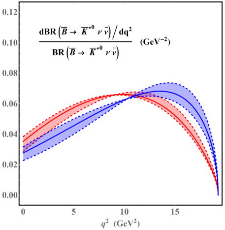
Figure 15: Theory predictions for the normalized differential $q^{2}$ distribution of $B\to K^{\ast}\,\nu_{\ell}\,\bar{\nu}_{\ell}$ with the semileptonic $B\to K^{\ast}$ form factors computed from the improved LCSR approach (pink band) and from the Lattice QCD simulation [2] (blue band).

$[q_{1}^{2},\,q_{2}^{2}]$    (${\rm in\,\,GeV}^{2}$)	$10^{6}\times\Delta{\cal BR}(q_{1}^{2},q_{2}^{2})$	$\,\,\,\Delta\,F_{L}(q_{1}^{2},q_{2}^{2})\,\,\,$
$[0.0,1.0]$	$0.41^{+0.10}_{-0.14}$	$0.95^{+0.01}_{-0.01}$
$[1.0,2.5]$	$0.72^{+0.19}_{-0.25}$	$0.84^{+0.02}_{-0.02}$
$[2.5,4.0]$	$0.83^{+0.25}_{-0.29}$	$0.74^{+0.03}_{-0.02}$
$[4.0,6.0]$	$1.25^{+0.42}_{-0.43}$	$0.65^{+0.03}_{-0.03}$
$[6.0,8.0]$	$1.36^{+0.52}_{-0.48}$	$0.56^{+0.03}_{-0.03}$
$[8.0,12.0]$	$2.84^{+1.26}_{-1.00}$	$0.46^{+0.02}_{-0.03}$
$[12.0,16.0]$	$2.46^{+1.30}_{-0.88}$	$0.36^{+0.02}_{-0.02}$
$\left[16.0,\,\,(m_{B}-m_{K^{\ast}})^{2}\right]$	$1.01^{+1.91}_{-1.25}$	$0.31^{+0.01}_{-0.01}$
$\left[0,\,\,(m_{B}-m_{K^{\ast}})^{2}\right]$	$10.88^{+4.62}_{-3.77}$	$0.52^{+0.03}_{-0.04}$

Table 8: Theory predictions for the $q^{2}$-binned observables $\Delta{\cal BR}$ and $\Delta\,F_{L}$ of the electroweak penguin $B\to K^{\ast}\,\nu_{\ell}\,\bar{\nu}_{\ell}$ decays with the heavy-to-light form factors computed from the $B$-meson LCSR approach and the $z$-series expansion.

We can proceed to define the differential longitudinal $K^{\ast}$ polarization fraction $F_{L}$ of the electroweak penguin $B\to K^{\ast}\,\nu_{\ell}\,\bar{\nu}_{\ell}$ decays

$$F_{L}(q^{2})=\frac{H_{A_{12}}(q^{2})}{H_{V}(q^{2})+H_{A_{1}}(q^{2})+H_{A_{12}}(q^{2})}\,.$$ (211)

In addition, we define the following two $q^{2}$-binned observables for the comparison with the future Belle II data

$$\Delta\,{\cal BR}(q_{1}^{2},q_{2}^{2}) = \tau_{B_{0}}\,\int_{q_{1}^{2}}^{q_{2}^{2}}\,dq^{2}\,{d\Gamma(B\to K^{\ast}\,\nu_{\ell}\,\bar{\nu}_{\ell})\over dq^{2}}\,,$$

$$\Delta\,F_{L}(q_{1}^{2},q_{2}^{2}) = \frac{\int_{q_{1}^{2}}^{q_{2}^{2}}\,dq^{2}\,\lambda^{3/2}(m_{B}^{2},m_{K^{\ast}}^{2},q^{2})\,H_{A_{12}}(q^{2})}{\int_{q_{1}^{2}}^{q_{2}^{2}}\,dq^{2}\,\lambda^{3/2}(m_{B}^{2},m_{K^{\ast}}^{2},q^{2})\,\left[H_{V}(q^{2})+H_{A_{1}}(q^{2})+H_{A_{12}}(q^{2})\right]}\,.$$ (212)

Our predictions for these two quantities with the choices of the $q^{2}$-intervals following [96] are presented in Table 8. Apparently, the theory uncertainties of the binned longitudinal $K^{\ast}$ polarization fractions are much reduced compared with the resulting predictions of $\Delta{\cal BR}$, due to the less sensitivity of the form-factor ratios to the precise shapes of the two-particle and three-particle $B$-meson distribution amplitudes.

6 Conclusion

In this paper we have presented improved QCD calculations of the twenty-one $B\to V$ ($V=\rho\,,\omega\,,K^{\ast}$) form factors by first implementing the hard-collinear factorization for the weak transition currents [41, 46, 42] and then computing the resulting $\rm{SCET_{I}}$ matrix elements from the LCSR technique with the HQET $B$-meson distribution amplitudes. The hard-collinear functions entering the factorization formulae for the $\rm{SCET_{I}}$ vacuum-to-$B$-meson correlation functions under discussion were determined at NLO in QCD for the leading-twist two-particle contributions, by employing the evanescent-operator approach with the dimensional regularization scheme. In particular, we demonstrated explicitly that the light-quark-mass terms appearing in the sum rules for the ${\rm A0}$-type SCET form factors $\xi_{\|,\,\perp}(n\cdot p)$, with the generic power counting scheme $m\sim\Lambda$, are not suppressed by any powers of $\Lambda/m_{b}$ in the heavy quark expansion as expected in [103]. We further computed the higher-twist corrections to the semileptonic $B\to V$ form factors from the two-particle and three-particle $B$-meson distribution amplitudes, up to the twist-six accuracy, with the same LCSR method at tree level in QCD. It turned out that the twist-five two-particle corrections to both the longitudinal and transverse $B\to V$ form factors were numerically dominant, in analogy to the previous observation for the semileptonic $B\to P$ form factors [22, 80]. However, we also noticed that the genuine three-particle higher-twist corrections were non-negligible for the transverse $B\to V$ form factors, in contrast to the pattern appeared in the longitudinal vector form factors. We proceeded to investigate the long-standing puzzles of the large-recoil symmetry breaking effects for the $B\to V$ form-factor ratios predicted by the QCD factorization approach and by the sum rule technique [4]. Following the standard strategy [87, 20], we extrapolated the LCSR calculations of the heavy-to-light form factors, with the two distinct models for the $B$-meson distribution amplitudes, toward the large $q^{2}$ region by virtue of the well-motivated $z$-series expansion.

We explored the phenomenological applications of the obtained predictions for $B$-meson decay form factors to the semileponic $B\to V\ell\nu_{\ell}$ decays as well as the electroweak penguin $B\to K^{\ast}\nu_{\ell}\bar{\nu}_{\ell}$ decays. The newly extracted interval of the CKM matrix element $|V_{ub}|=\left(3.05\,{}^{+0.67}_{-0.52}\big{|}_{\rm th.}\,{}^{+0.19}_{-0.20}\big{|}_{\rm exp.}\right)\times 10^{-3}$ from the exclusive process $B\to\rho\ell\nu_{\ell}$ is in agreement with the previous determination from $B\to\pi\ell\nu_{\ell}$ applying the same computational framework, but the analogous determination from $B\to\omega\ell\nu_{\ell}$ yields somewhat smaller values of $|V_{ub}|$, albeit with the sizeable theory uncertainties mainly due to the limited knowledge of the small $\omega$-behaviours of the two-particle $B$-meson distribution amplitude $\phi_{B}^{\pm}(\omega,\mu)$. The two $q^{2}$-binned observables $\Delta\,{\cal BR}$ and $\Delta\,F_{L}$ for the exclusive rare $B\to K^{\ast}\,\nu_{\ell}\,\bar{\nu}_{\ell}$ decays were further predicted for the sake of hunting for new physics beyond the SM at the Belle II experiment [96].

Future developments of QCD calculations of $B\to V$ form factors at large hadronic recoil can be pushed forward both conceptually and technically. First, it will be of wide interest to carry out the two-particle and three-particle higher-twist contributions to the semileptonic $B\to V$ form factors, up to the twist-six accuracy, at NLO in QCD in order to verify explicitly that the higher-Fock state contributions of both the $B$-meson and the energetic vector meson generate the leading-power effects in the heavy quark expansion as demonstrated in [7]. The computational challenges of determining the hard-collinear functions entering the $\rm{SCET_{I}}$ factorization formulae for the vacuum-to-$B$-meson correlation functions originate from the non-trivial mixing of the different light-ray HQET operators under renormalization beyond the twist-four accuracy [43], making the infrared subtraction of the perturbative matching procedure tediously in dimensional regularization. In addition, constructing the meaningful constraints for the higher-twist $B$-meson distribution amplitudes from the QCD equations of motion beyond the LO in QCD are complicated by the appearance of the light-cone divergences. Second, improving theory calculations for the higher-dimensional local HQET matrix elements $\lambda_{E}^{2}(\mu)$ and $\lambda_{H}^{2}(\mu)$ will be of value for reducing the parametric uncertainties on the phenomenological aspect, in view of the significant discrepancies of the two independent QCD sum rule calculations presented in [52] and [69] . However, evaluating the NLO QCD correction to the leading-power contribution in the framework of QCD sum rules will also necessitate challenging computations of the two-point HQET diagrams at three loops. Third, implementing a complete NLL QCD resummation for the enhanced logarithms due to the RG evolutions of both the short-distance Wilson coefficients and the leading-twist $B$-meson distribution amplitude [59] is essential to the precision calculations of the semileptonic $B\to V$ form factors, but it is also a technically demanding task to achieve this goal in a full analytical form. It will be probably more promising to derive the NLL resummation improved SCET factorization formula for the radiative leptonic $B$-meson decays in this respect. To summarize, we expect interesting extensions of our work for deepening our understanding of the factorization and resummation properties of heavy-to-light $B$-meson decay form factors in QCD.

Acknowledgements

C.D.L is supported in part by the National Natural Science Foundation of China (NSFC) with Grant No. 11521505 and 11621131001. The work of Y.L.S is supported by the Natural Science Foundation of Shandong Province, China under Grant No. ZR2015AQ006. Y.M.W acknowledges support from the National Youth Thousand Talents Program, the Youth Hundred Academic Leaders Program of Nankai University, and the NSFC with Grant No. 11675082 and 11735010. The work of Y.B.W is supported in part by the NSFC with Grant No. 11847238. This work was also supported in part by the Mainz Institute for Theoretical Physics (MITP) of the Johannes Gutenberg University.

Appendix A Hard functions for the SCET currents at ${\cal O}(\alpha_{s})$

Here we collect the hard matching coefficient functions for the A0-type and B-type ${\rm SCET_{I}}$ currents entering the factorization formulae (8) for the semileptonic $B\to V$ form factors.

$$C_{f_{+}}^{\rm(A0)} = 1+{\alpha_{s}\,C_{F}\over 4\,\pi}\,\bigg{\{}-2\,\ln^{2}\left({r\over\hat{\mu}}\right)+5\,\ln\left({r\over\hat{\mu}}\right)-2\,{\rm Li}_{2}(1-r)-3\,\ln r-{\pi^{2}\over 12}-6\bigg{\}},$$ (213)

$$C_{f_{0}}^{\rm(A0)} = 1+{\alpha_{s}\,C_{F}\over 4\,\pi}\,\bigg{\{}-2\,\ln^{2}\left({r\over\hat{\mu}}\right)+5\,\ln\left({r\over\hat{\mu}}\right)-2\,{\rm Li}_{2}(1-r)-{3-5\,r\over 1-r}\,\ln r$$ (214)

$$-{\pi^{2}\over 12}-4\bigg{\}}\,,$$

$$C_{f_{T}}^{\rm(A0)} = 1+{\alpha_{s}\,C_{F}\over 4\,\pi}\,\bigg{\{}-2\,\ln\hat{\nu}-2\,\ln^{2}\left({r\over\hat{\mu}}\right)+5\,\ln\left({r\over\hat{\mu}}\right)-2\,{\rm Li}_{2}(1-r)-{3-r\over 1-r}\,\ln r$$ (215)

$$-{\pi^{2}\over 12}-6\bigg{\}}\,,$$

$$C_{V}^{\rm(A0)} = 1+{\alpha_{s}\,C_{F}\over 4\,\pi}\,\bigg{\{}-2\,\ln^{2}\left({r\over\hat{\mu}}\right)+5\,\ln\left({r\over\hat{\mu}}\right)-2\,{\rm Li}_{2}(1-r)-{3-2\,r\over 1-r}\,\ln r$$ (216)

$$-{\pi^{2}\over 12}-6\bigg{\}}\,,$$

$$C_{T_{1}}^{\rm(A0)} = 1+{\alpha_{s}\,C_{F}\over 4\,\pi}\,\bigg{\{}-2\,\ln\hat{\nu}-2\,\ln^{2}\left({r\over\hat{\mu}}\right)+5\,\ln\left({r\over\hat{\mu}}\right)-2\,{\rm Li}_{2}(1-r)-3\,\ln r$$ (217)

$$-{\pi^{2}\over 12}-6\bigg{\}}\,,$$

$$C_{f_{+}}^{\rm(B1)} = \left(-2+{1\over r}\right)+{\cal O}(\alpha_{s})\,,\qquad C_{f_{0}}^{\rm(B1)}=\left(-{1\over r}\right)+{\cal O}(\alpha_{s})\,,$$ (218)

$$C_{f_{T}}^{\rm(B1)} = \left({1\over r}\right)+{\cal O}(\alpha_{s})\,,\qquad C_{V}^{\rm(B1)}=0+{\cal O}(\alpha_{s})\,,\qquad C_{T_{1}}^{\rm(B1)}=-1+{\cal O}(\alpha_{s})\,,$$ (219)

where we have introduced the variables

$$r={n\cdot p\over m_{b}}\,,\qquad\hat{\mu}={\mu\over m_{b}}\,,\qquad\hat{\nu}={\nu\over m_{b}}\,.$$ (220)

Appendix B $B$-meson distribution amplitudes

In this appendix we collect the explicit expressions for two different models of the two-particle and three-particle $B$-meson distribution amplitudes employed in our numerical study of the obtained sum rules for $B\to V$ form factors.

• Exponential model:

  $$\phi_{B}^{+,\,\rm exp}(\omega,\mu) = {\omega\over\omega_{0}^{2}}\,e^{-\omega/\omega_{0}}\,,$$

  $$\phi_{B}^{-,\,\rm exp}(\omega,\mu) = {1\over\omega_{0}}\,e^{-\omega/\omega_{0}}-{\lambda_{E}^{2}-\lambda_{H}^{2}\over 9\,\omega_{0}^{3}}\,\left[1-2\,\left({\omega\over\omega_{0}}\right)+{1\over 2}\,\left({\omega\over\omega_{0}}\right)^{2}\right]\,e^{-\omega/\omega_{0}}\,,$$

  $$\hat{g}_{B}^{-,\,\rm exp}(\omega,\mu) = \omega\,\left\{{3\over 4}-{\lambda_{E}^{2}-\lambda_{H}^{2}\over 12\,\omega_{0}^{2}}\,\left[1-\left({\omega\over\omega_{0}}\right)+{1\over 3}\,\left({\omega\over\omega_{0}}\right)^{2}\right]\right\}\,e^{-\omega/\omega_{0}}\,,$$

  $$\Phi_{3}^{\rm exp}(\omega_{1},\omega_{2},\mu) = {\lambda_{E}^{2}-\lambda_{H}^{2}\over 6\,\omega_{0}^{5}}\,\omega_{1}\,\omega_{2}^{2}\,e^{-(\omega_{1}+\omega_{2})/\omega_{0}}\,,$$

  $$\Phi_{4}^{\rm exp}(\omega_{1},\omega_{2},\mu) = {\lambda_{E}^{2}+\lambda_{H}^{2}\over 6\,\omega_{0}^{4}}\,\omega_{2}^{2}\,e^{-(\omega_{1}+\omega_{2})/\omega_{0}}\,,$$

  $$\Psi_{4}^{\rm exp}(\omega_{1},\omega_{2},\mu) = {\lambda_{E}^{2}\over 3\,\omega_{0}^{4}}\,\omega_{1}\,\omega_{2}\,e^{-(\omega_{1}+\omega_{2})/\omega_{0}}\,,$$

  $$\tilde{\Psi}_{4}^{\rm exp}(\omega_{1},\omega_{2},\mu) = {\lambda_{H}^{2}\over 3\,\omega_{0}^{4}}\,\omega_{1}\,\omega_{2}\,e^{-(\omega_{1}+\omega_{2})/\omega_{0}}\,,$$

  $$\Phi_{5}^{\rm exp}(\omega_{1},\omega_{2},\mu) = {\lambda_{E}^{2}+\lambda_{H}^{2}\over 3\,\omega_{0}^{3}}\,\omega_{1}\,e^{-(\omega_{1}+\omega_{2})/\omega_{0}}\,,$$

  $$\Psi_{5}^{\rm exp}(\omega_{1},\omega_{2},\mu) = -{\lambda_{E}^{2}\over 3\,\omega_{0}^{3}}\,\omega_{2}\,e^{-(\omega_{1}+\omega_{2})/\omega_{0}}\,,$$

  $$\tilde{\Psi}_{5}^{\rm exp}(\omega_{1},\omega_{2},\mu) = -{\lambda_{H}^{2}\over 3\,\omega_{0}^{3}}\,\omega_{2}\,e^{-(\omega_{1}+\omega_{2})/\omega_{0}}\,,$$

  $$\Phi_{6}^{\rm exp}(\omega_{1},\omega_{2},\mu) = {\lambda_{E}^{2}-\lambda_{H}^{2}\over 3\,\omega_{0}^{2}}\,e^{-(\omega_{1}+\omega_{2})/\omega_{0}}\,.$$ (221)

  The classical QCD equations of motion further imply the following relations of the HQET parameters appearing in this specifical model [43]

  $$\omega_{0}=\lambda_{B}={2\over 3}\,\bar{\Lambda}\,,\qquad 2\,\bar{\Lambda}^{2}=2\,\lambda_{E}^{2}+\lambda_{H}^{2}\,,$$ (222)

  so that only two of the three non-perturbative parameters $\lambda_{B}$, $\lambda_{E}^{2}$ and $\lambda_{H}^{2}$ are independent of each other at tree level.

• Local-duality model:

  $$\phi_{B}^{+,\rm LD}(\omega,\mu) = {5\over 8\,\omega_{0}^{5}}\,\omega(2\,\omega_{0}-\omega)^{3}\,\theta(2\,\omega_{0}-\omega)\,,$$

  $$\phi_{B}^{-,\rm LD}(\omega,\mu) = {5(2\,\omega_{0}-\omega)^{2}\over 192\,\omega_{0}^{5}}\,\bigg{\{}6\,(2\,\omega_{0}-\omega)^{2}-{7\,(\lambda_{E}^{2}-\lambda_{H}^{2})\over\omega_{0}^{2}}\,(15\,\omega^{2}-20\,\omega\,\omega_{0}+4\,\omega_{0}^{2})\bigg{\}}\,$$

  $$\times\,\theta(2\,\omega_{0}-\omega)\,,$$

  $$\hat{g}_{B}^{-,\rm LD}(\omega,\mu) = {\omega\,(2\,\omega_{0}-\omega)^{3}\over\omega_{0}^{5}}\,\bigg{\{}-{35\,(\lambda_{E}^{2}-\lambda_{H}^{2})\over 1536}\,\left[4-12\,\left({\omega\over\omega_{0}}\right)+11\,\left({\omega\over\omega_{0}}\right)^{2}\right]$$

  $$+{5\over 256}\,(2\,\omega_{0}-\omega)^{2}\bigg{\}}\,\,\theta(2\,\omega_{0}-\omega)\,,$$

  $$\Phi_{3}^{\rm LD}(\omega_{1},\omega_{2},\mu) = {105\,(\lambda_{E}^{2}-\lambda_{H}^{2})\over 8\,\omega_{0}^{7}}\,\omega_{1}\,\omega_{2}^{2}\,\left(\omega_{0}-{\omega_{1}+\omega_{2}\over 2}\right)^{2}\,\theta(2\,\omega_{0}-\omega_{1}-\omega_{2})\,,$$

  $$\Phi_{4}^{\rm LD}(\omega_{1},\omega_{2},\mu) = {35\,(\lambda_{E}^{2}+\lambda_{H}^{2})\over 4\,\omega_{0}^{7}}\,\omega_{2}^{2}\,\left(\omega_{0}-{\omega_{1}+\omega_{2}\over 2}\right)^{3}\,\theta(2\,\omega_{0}-\omega_{1}-\omega_{2})\,,$$

  $$\Psi_{4}^{\rm LD}(\omega_{1},\omega_{2},\mu) = {35\,\lambda_{E}^{2}\over 2\,\omega_{0}^{7}}\,\omega_{1}\,\omega_{2}\,\left(\omega_{0}-{\omega_{1}+\omega_{2}\over 2}\right)^{3}\,\theta(2\,\omega_{0}-\omega_{1}-\omega_{2})\,,$$

  $$\tilde{\Psi}_{4}^{\rm LD}(\omega_{1},\omega_{2},\mu) = {35\,\lambda_{H}^{2}\over 2\,\omega_{0}^{7}}\,\omega_{1}\,\omega_{2}\,\left(\omega_{0}-{\omega_{1}+\omega_{2}\over 2}\right)^{3}\,\theta(2\,\omega_{0}-\omega_{1}-\omega_{2})\,,$$

  $$\Phi_{5}^{\rm LD}(\omega_{1},\omega_{2},\mu) = {35\over 64}\,(\lambda_{E}^{2}+\lambda_{H}^{2})\,{\omega_{1}\over\omega_{0}^{7}}\,(2\,\omega_{0}-\omega_{1}-\omega_{2})^{4}\,\theta(2\,\omega_{0}-\omega_{1}-\omega_{2})\,,$$

  $$\Psi_{5}^{\rm LD}(\omega_{1},\omega_{2},\mu) = -{35\over 64}\,\lambda_{E}^{2}\,{\omega_{2}\over\omega_{0}^{7}}\,(2\,\omega_{0}-\omega_{1}-\omega_{2})^{4}\,\theta(2\,\omega_{0}-\omega_{1}-\omega_{2})\,,$$

  $$\tilde{\Psi}_{5}^{\rm LD}(\omega_{1},\omega_{2},\mu) = -{35\over 64}\,\lambda_{H}^{2}\,{\omega_{2}\over\omega_{0}^{7}}\,(2\,\omega_{0}-\omega_{1}-\omega_{2})^{4}\,\theta(2\,\omega_{0}-\omega_{1}-\omega_{2})\,,$$

  $$\Phi_{6}^{\rm LD}(\omega_{1},\omega_{2},\mu) = {7\over 64}\,(\lambda_{E}^{2}-\lambda_{H}^{2})\,{1\over\omega_{0}^{7}}\,(2\,\omega_{0}-\omega_{1}-\omega_{2})^{5}\,\theta(2\,\omega_{0}-\omega_{1}-\omega_{2})\,.$$ (223)

  Analogously, the HQET parameters for the local-duality model also satisfy nontrivial constraints due to QCD equations of motion [43]

  $$\omega_{0}={5\over 2}\,\lambda_{B}=2\,\bar{\Lambda}\,,\qquad 6\,{\bar{\Lambda}}^{2}=7\,(2\,\lambda_{E}^{2}+\lambda_{H}^{2})\,.$$ (224)

References

- [1] R. R. Horgan, Z. Liu, S. Meinel and M. Wingate, Phys. Rev. D 89 (2014) no.9, 094501 [arXiv:1310.3722 [hep-lat]].
- [2] R. R. Horgan, Z. Liu, S. Meinel and M. Wingate, PoS LATTICE 2014 (2015) 372 [arXiv:1501.00367 [hep-lat]].
- [3] A. Bazavov et al. [MILC Collaboration], Rev. Mod. Phys. 82 (2010) 1349 [arXiv:0903.3598 [hep-lat]].
- [4] M. Beneke and T. Feldmann, Nucl. Phys. B 592 (2001) 3 [hep-ph/0008255].
- [5] C. W. Bauer, D. Pirjol and I. W. Stewart, Phys. Rev. D 67 (2003) 071502 [hep-ph/0211069].
- [6] M. Beneke, A. P. Chapovsky, M. Diehl and T. Feldmann, Nucl. Phys. B 643 (2002) 431 [hep-ph/0206152].
- [7] M. Beneke and T. Feldmann, Nucl. Phys. B 685 (2004) 249 [hep-ph/0311335].
- [8] P. Ball and V. M. Braun, Phys. Rev. D 55 (1997) 5561 [hep-ph/9701238].
- [9] P. Ball and V. M. Braun, Phys. Rev. D 58 (1998) 094016 [hep-ph/9805422].
- [10] P. Ball and R. Zwicky, Phys. Rev. D 71 (2005) 014029 [hep-ph/0412079].
- [11] A. Bharucha, D. M. Straub and R. Zwicky, JHEP 1608 (2016) 098 [arXiv:1503.05534 [hep-ph]].
- [12] U. G. Meißner and W. Wang, Phys. Lett. B 730 (2014) 336 [arXiv:1312.3087 [hep-ph]].
- [13] C. Hambrock and A. Khodjamirian, Nucl. Phys. B 905 (2016) 373 [arXiv:1511.02509 [hep-ph]].
- [14] S. Cheng, A. Khodjamirian and J. Virto, Phys. Rev. D 96 (2017) 051901 [arXiv:1709.00173 [hep-ph]].
- [15] W. Cheng, X. G. Wu, R. Y. Zhou and H. B. Fu, Phys. Rev. D 98 (2018) 096013 [arXiv:1808.10775 [hep-ph]].
- [16] A. Khodjamirian, T. Mannel and N. Offen, Phys. Lett. B 620 (2005) 52 [hep-ph/0504091].
- [17] A. Khodjamirian, T. Mannel and N. Offen, Phys. Rev. D 75 (2007) 054013 [hep-ph/0611193].
- [18] A. Khodjamirian, T. Mannel, A. A. Pivovarov and Y.-M. Wang, JHEP 1009 (2010) 089 [arXiv:1006.4945 [hep-ph]].
- [19] A. Khodjamirian, T. Mannel and Y. M. Wang, JHEP 1302 (2013) 010 [arXiv:1211.0234 [hep-ph]].
- [20] Y. M. Wang and Y. L. Shen, Nucl. Phys. B 898 (2015) 563 [arXiv:1506.00667 [hep-ph]].
- [21] Y. M. Wang, Y. B. Wei, Y. L. Shen and C. D. Lü, JHEP 1706 (2017) 062 [arXiv:1701.06810 [hep-ph]].
- [22] C. D. Lü, Y. L. Shen, Y. M. Wang and Y. B. Wei, JHEP 1901 (2019) 024 [arXiv:1810.00819 [hep-ph]].
- [23] M. Beneke and V. A. Smirnov, Nucl. Phys. B 522 (1998) 321 [hep-ph/9711391].
- [24] V. A. Smirnov, Applied asymptotic expansions in momenta and masses, Springer Tracts Mod. Phys. 177 (2002) 1.
- [25] F. De Fazio, T. Feldmann and T. Hurth, Nucl. Phys. B 733 (2006) 1 Erratum: [Nucl. Phys. B 800 (2008) 405] [hep-ph/0504088].
- [26] F. De Fazio, T. Feldmann and T. Hurth, JHEP 0802 (2008) 031 [arXiv:0711.3999 [hep-ph]].
- [27] Y. Y. Keum, H. N. Li and A. I. Sanda, Phys. Rev. D 63 (2001) 054008 [hep-ph/0004173].
- [28] C. D. Lü, K. Ukai and M. Z. Yang, Phys. Rev. D 63 (2001) 074009 [hep-ph/0004213].
- [29] S. Nandi and H. n. Li, Phys. Rev. D 76 (2007) 034008 [arXiv:0704.3790 [hep-ph]].
- [30] H. n. Li, Y. L. Shen, Y. M. Wang and H. Zou, Phys. Rev. D 83 (2011) 054029 [arXiv:1012.4098 [hep-ph]].
- [31] H. n. Li, Y. L. Shen and Y. M. Wang, Phys. Rev. D 85 (2012) 074004 [arXiv:1201.5066 [hep-ph]].
- [32] H. N. Li, Y. L. Shen and Y. M. Wang, JHEP 1302 (2013) 008 [arXiv:1210.2978 [hep-ph]].
- [33] H. N. Li, Y. L. Shen and Y. M. Wang, JHEP 1401 (2014) 004 [arXiv:1310.3672 [hep-ph]].
- [34] J. C. Collins and D. E. Soper, Nucl. Phys. B 193 (1981) 381 Erratum: [Nucl. Phys. B 213 (1983) 545].
- [35] J. C. Collins, D. E. Soper and G. F. Sterman, Nucl. Phys. B 250 (1985) 199.
- [36] J. Collins, Foundations of Perturbative QCD, Camb. Monogr. Part. Phys. Nucl. Phys. Cosmol. 32 (2011) 1.
- [37] H. n. Li and Y. M. Wang, JHEP 1506 (2015) 013 [arXiv:1410.7274 [hep-ph]].
- [38] Y. M. Wang, EPJ Web Conf. 112 (2016) 01021 [arXiv:1512.08374 [hep-ph]].
- [39] M. J. Dugan and B. Grinstein, Phys. Lett. B 256 (1991) 239.
- [40] S. Herrlich and U. Nierste, Nucl. Phys. B 455 (1995) 39 [hep-ph/9412375].
- [41] R. J. Hill, T. Becher, S. J. Lee and M. Neubert, JHEP 0407 (2004) 081 [hep-ph/0404217].
- [42] M. Beneke and D. S. Yang, Nucl. Phys. B 736 (2006) 34 [hep-ph/0508250].
- [43] V. M. Braun, Y. Ji and A. N. Manashov, JHEP 1705 (2017) 022 [arXiv:1703.02446 [hep-ph]].
- [44] H. Kawamura, J. Kodaira, C. F. Qiao and K. Tanaka, Phys. Lett. B 523 (2001) 111; Erratum: [Phys. Lett. B 536 (2002) 344] [hep-ph/0109181].
- [45] M. Beneke, T. Huber and X.-Q. Li, Nucl. Phys. B 811 (2009) 77 [arXiv:0810.1230 [hep-ph]].
- [46] T. Becher and R. J. Hill, JHEP 0410 (2004) 055 [hep-ph/0408344].
- [47] B. O. Lange and M. Neubert, Nucl. Phys. B 690 (2004) 249 Erratum: [Nucl. Phys. B 723 (2005) 201] [hep-ph/0311345].
- [48] C. W. Bauer, S. Fleming, D. Pirjol and I. W. Stewart, Phys. Rev. D 63 (2001) 114020 [hep-ph/0011336].
- [49] M. Beneke, Y. Kiyo and D. S. Yang, Nucl. Phys. B 692 (2004) 232 [hep-ph/0402241].
- [50] M. Beneke and T. Feldmann, Phys. Lett. B 553 (2003) 267 [hep-ph/0211358].
- [51] G. Burdman and G. Hiller, Phys. Rev. D 63 (2001) 113008 [hep-ph/0011266].
- [52] A. G. Grozin and M. Neubert, Phys. Rev. D 55 (1997) 272 [hep-ph/9607366].
- [53] M. Beneke, M. Garny, R. Szafron and J. Wang, JHEP 1811 (2018) 112 [arXiv:1808.04742 [hep-ph]].
- [54] Y. M. Wang and Y. L. Shen, JHEP 1602 (2016) 179 [arXiv:1511.09036 [hep-ph]].
- [55] M. Beneke and J. Rohrwild, Eur. Phys. J. C 71 (2011) 1818 [arXiv:1110.3228 [hep-ph]].
- [56] X. D. Ji and M. J. Musolf, Phys. Lett. B 257 (1991) 409.
- [57] D. J. Broadhurst and A. G. Grozin, Phys. Lett. B 267 (1991) 105 [hep-ph/9908362].
- [58] Y. M. Wang, JHEP 1609 (2016) 159 [arXiv:1606.03080 [hep-ph]].
- [59] V. M. Braun, Y. Ji and A. N. Manashov, arXiv:1905.04498 [hep-ph].
- [60] L. J. Reinders, H. Rubinstein and S. Yazaki, Phys. Rept. 127 (1985) 1.
- [61] Y. M. Wang and Y. L. Shen, JHEP 1712 (2017) 037 [arXiv:1706.05680 [hep-ph]].
- [62] G. Bell, M. Beneke, T. Huber and X. Q. Li, Nucl. Phys. B 843 (2011) 143 [arXiv:1007.3758 [hep-ph]].
- [63] I. I. Balitsky and V. M. Braun, Nucl. Phys. B 311 (1989) 541.
- [64] A. V. Rusov, Eur. Phys. J. C 77 442 (2017) [arXiv:1705.01929 [hep-ph]].
- [65] M. Beneke, V. M. Braun, Y. Ji and Y. B. Wei, JHEP 1807 (2018) 154 [arXiv:1804.04962 [hep-ph]].
- [66] G. Bell, T. Feldmann, Y. M. Wang and M. W. Y. Yip, JHEP 1311 (2013) 191 [arXiv:1308.6114 [hep-ph]].
- [67] V. M. Braun, D. Y. Ivanov and G. P. Korchemsky, Phys. Rev. D 69 (2004) 034014 [hep-ph/0309330].
- [68] A. G. Grozin and M. Neubert, Nucl. Phys. B 495 (1997) 81 [hep-ph/9701262].
- [69] T. Nishikawa and K. Tanaka, Nucl. Phys. B 879 (2014) 110 [arXiv:1109.6786 [hep-ph]].
- [70] S. Aoki et al., Eur. Phys. J. C 77 (2017) 112 [arXiv:1607.00299 [hep-lat]].
- [71] C. Allton et al. [RBC-UKQCD Collaboration], Phys. Rev. D 78 (2008) 114509 [arXiv:0804.0473 [hep-lat]].
- [72] P. Ball, V. M. Braun, Y. Koike and K. Tanaka, Nucl. Phys. B 529 (1998) 323 [hep-ph/9802299].
- [73] P. Ball and V. M. Braun, Phys. Rev. D 54 (1996) 2182 [hep-ph/9602323].
- [74] M. Beneke, A. Maier, J. Piclum and T. Rauh, Nucl. Phys. B 891 (2015) 42 [arXiv:1411.3132 [hep-ph]].
- [75] B. Dehnadi, A. H. Hoang and V. Mateu, JHEP 1508 (2015) 155 [arXiv:1504.07638 [hep-ph]].
- [76] V. Mateu and P. G. Ortega, JHEP 1801 (2018) 122 [arXiv:1711.05755 [hep-ph]].
- [77] M. Tanabashi et al. [Particle Data Group], Phys. Rev. D 98 (2018) 030001.
- [78] Y. M. Wang and Y. L. Shen, JHEP 1805 (2018) 184 [arXiv:1803.06667 [hep-ph]].
- [79] M. Beneke and M. Neubert, Nucl. Phys. B 675 (2003) 333 [hep-ph/0308039].
- [80] N. Gubernari, A. Kokulu and D. van Dyk, JHEP 1901 (2019) 150 [arXiv:1811.00983 [hep-ph]].
- [81] M. Beneke, eConf C 0610161 (2006) 030 [Nucl. Phys. Proc. Suppl. 170 (2007) 57] [hep-ph/0612353].
- [82] S. Wandzura and F. Wilczek, Phys. Lett. 72B (1977) 195.
- [83] C. Bourrely, B. Machet and E. de Rafael, Nucl. Phys. B 189 (1981) 157.
- [84] A. Khodjamirian and A. V. Rusov, JHEP 1708 (2017) 112 [arXiv:1703.04765 [hep-ph]].
- [85] C. Bourrely, I. Caprini and L. Lellouch, Phys. Rev. D 79 (2009) 013008; Erratum: [Phys. Rev. D 82 (2010) 099902] [arXiv:0807.2722 [hep-ph]].
- [86] C. G. Boyd, B. Grinstein and R. F. Lebed, Phys. Lett. B 353 (1995) 306 [hep-ph/9504235].
- [87] A. Khodjamirian, T. Mannel, N. Offen and Y.-M. Wang, Phys. Rev. D 83 (2011) 094031 [arXiv:1103.2655 [hep-ph]].
- [88] W. A. Bardeen, E. J. Eichten and C. T. Hill, Phys. Rev. D 68 (2003) 054024 [hep-ph/0305049].
- [89] A. Bharucha, T. Feldmann and M. Wick, JHEP 1009 (2010) 090 [arXiv:1004.3249 [hep-ph]].
- [90] D. Bigi and P. Gambino, Phys. Rev. D 94 (2016) 094008 [arXiv:1606.08030 [hep-ph]].
- [91] S. W. Bosch and G. Buchalla, JHEP 0501 (2005) 035 [hep-ph/0408231].
- [92] M. Beneke, T. Feldmann and D. Seidel, Eur. Phys. J. C 41 (2005) 173 [hep-ph/0412400].
- [93] P. del Amo Sanchez et al. [BaBar Collaboration], Phys. Rev. D 83 (2011) 032007 [arXiv:1005.3288 [hep-ex]].
- [94] A. Sibidanov et al. [Belle Collaboration], Phys. Rev. D 88 (2013) 032005 [arXiv:1306.2781 [hep-ex]].
- [95] J. P. Lees et al. [BaBar Collaboration], Phys. Rev. D 86 (2012) 092004 [arXiv:1208.1253 [hep-ex]].
- [96] E. Kou et al. [Belle-II Collaboration], “The Belle II Physics Book,” arXiv:1808.10567 [hep-ex].
- [97] A. J. Buras, J. Girrbach-Noe, C. Niehoff and D. M. Straub, JHEP 1502 (2015) 184 [arXiv:1409.4557 [hep-ph]].
- [98] T. Inami and C. S. Lim, Prog. Theor. Phys. 65 (1981) 297; Erratum: [Prog. Theor. Phys. 65 (1981) 1772].
- [99] G. Buchalla and A. J. Buras, Nucl. Phys. B 548 (1999) 309 [hep-ph/9901288].
- [100] G. Buchalla and A. J. Buras, Nucl. Phys. B 398 (1993) 285.
- [101] M. Misiak and J. Urban, Phys. Lett. B 451 (1999) 161 [hep-ph/9901278].
- [102] J. Brod, M. Gorbahn and E. Stamou, Phys. Rev. D 83 (2011) 034030 [arXiv:1009.0947 [hep-ph]].
- [103] A. K. Leibovich, Z. Ligeti and M. B. Wise, Phys. Lett. B 564 (2003) 231 [hep-ph/0303099].