Structural models based on 3D constitutive laws: variational structure and numerical solution

Abstract

In all structural models, the section or fiber response is a relation between the strain measures and the stress resultants. This relation can only be expressed in a simple analytical form when the material response is linear elastic. For other, more complex and interesting situations, kinematic and kinetic hypotheses need to be invoked, and a constrained three-dimensional constitutive relation has to be employed at every point of the section in order to implement non-linear and dissipative constitutive laws into dimensionally reduced structural models. In this article we explain in which sense reduced constitutive models can be expressed as minimization problems, helping to formulate the global equilibrium as a single optimization problem. Casting the problem this way has implications from the mathematical and numerical points of view, naturally defining error indicators. General purpose solution algorithms for constrained material response, with and without optimization character, are discussed and provided in an open-source library.

1 Introduction

In linear and nonlinear structural theories (including bars, beams, plates, membranes, shells, etc.), the kinematic definitions and the equilibrium equations need to be closed with a relation between the strain measures and the stress resultants, possibly with time-dependent and dissipative effects. In the simplest situations, often restricted to the linear elastic case, there exists an analytical expression that relates stresses and strain resultants, leading to well-known equations that have been employed for decades in structural analyses (see [1, 2, 3], for example, among many books fully describing this process).

Structural analyses involving nonlinear elastic or inelastic materials can rarely make use of section response laws and must, therefore, relie directly on three-dimensional constitutive laws evaluated at every point of the cross section. Such an evaluation is complicated due to the fact that every structural theory constrains, from its outset, the kind of strains and stresses that are allowed on the sections. The hypotheses imply that the constitutive response of these material points is constrained and its evaluation is rarely possible by analytical means.

These constrained constitutive laws must provide, given a proper subset of the strain components and knowing that some stress components vanish, the remaining parts of the strain and stress tensors. Numerical methods designed to solve this problem are iterative by nature, since, except for the linear elastic case, the strain-stress relations are often implicit and nonlinear. Standard Newton-Raphson iterative methods – or related ones – have been proposed for this purpose in the past [4, 5, 6, 7].

Newton-like methods solve the constrained constitutive problem in a fast and robust fashion. By focusing on the nonlinear (and constrained) strain-stress relations, however, they fail to notice that there is an underlying variational structure behind the problem. In this article we reveal the precise meaning of this framework, and identify the form of the energy functional involved. Such a characterization allows to show that the equilibrium problem of structures, even when the section constitutive law is evaluated pointwise from contrained three-dimensional models, has a global variational character.

This assertion has at least three consequences. First, from the theoretical point of view, theorems for the existence of solutions can now be derived based on minimizing sequences and properties of functionals, even in the constrained case. Second, for more pragmatic reasons, numerical optimization methods can be used to solve the global problem and local constitutive relations, for example of nonlinear conjugate gradient type. And third, since a single energy functional is shown to be the quantity to minimize for a given solution, it provides a natural error indicator for Galerkin-type approximations. The first of these three implications falls outside the scope of the current work, but the second and the third point are discussed and exemplified in Sections 4 and 5.

The setting employed for the derivations in this article is that of linearized kinematics and nonlinear materials with internal variables. This framework is general enough to accommodate many problems of interest, and can be extended, in a fairly straightforward manner to include geometrical nonlinearities. Due to the similarities with the small strain case, the details of such generalization are not worked out in this article, although both small and finite strain simulation examples will be provided.

The way that we choose to deal with material nonlinearities, rate and history effects is by means of incremental potentials [8]. With them, a variational structure is preserved even for problems involving plasticity, viscoelasticity, etc., as long as this is interpreted in an incremental fashion. Such ideas, widespread in Computational Mechanics, are extended by our results to structural models of inelastic materials.

The remainder of this article is organized in the following way. In Section 2 we describe structural models in an abstract way that can encompass all types. In this completely general setting, we introduce the connection between the section response and the constrained material constitutive law. The underlying variational setting is discussed in Section 3 by revealing that there is a compatible minimization structure at the level of material point, section, and structural member. In addition to the theoretical advantages of the formulation, as already mentioned, some numerical implications are studied in Section 4 and illustrated by means of examples in Section 5. Section 6 closes the article summarizing the main findings.

As will be detailed in Section 4, we classify two types of methods that can be employed to solve numerically the constrained or reduced constitutive model. The material open-source library MUESLI [9] implements both, and readers can access it to verify the details of the numerical implementation.

2 From structural models to 3D, and back

We explore in this section the relationship between the mechanics of three-dimensional solids and structural theories. There are many interesting points of view for this analysis, including asymptotic behavior, model reduction, numerical discretization, etc., but we restrict our exposition to those features that help to explain the central point of this article: how three-dimensional material constitutive laws can be employed to formulate section response relations. We address fully inelastic materials, although we restrict our exposition to linearized kinematics. Extension to the geometrically nonlinear regime follows in a relatively straightforward manner and, in fact, we will employ it in some of the simulations of Section 5.

2.1 Abstract structural models

To accommodate all potential structural models in our analysis we present them next in an abstract way. The notation is general enough to encompass bars, rods, plates, etc. and any other model based on structural strain measures and stress resultants. When possible, we will make the connection to specific models, but the goal is to set up a common framework to establish the relation with three-dimensional material models in a single form. We proceed in this line by introducing six crucial elements of every structural theory:

i) Geometry

The reference configuration of any structural model can be defined geometrically as a product bundle $\mathcal{S}=\mathcal{M}\times\mathcal{F}$, where the set $\mathcal{M}$ is referred to as the base manifold and $\mathcal{F}$ is the fiber [10]. Both sets are assumed to be smooth manifolds endowed with measures $\mu(\mathcal{M})$ and $\mu(\mathcal{F})$, respectively. Key to any product manifold, there exist surjective projections $\pi_{M}:\mathcal{S}\to\mathcal{M}$ and $\pi_{F}:\mathcal{S}\to\mathcal{F}$. Any point on the model has coordinates $(\bm{x},\bm{\xi})$ with $\bm{x}\in\mathcal{M}$ and $\bm{\xi}\in\mathcal{F}$. For example, if $\mathcal{S}$ is a shell, the base manifold is a two-dimensional (smooth) surface that corresponds to the shell midsurface and the fiber is a segment through the thickness. When $\mathcal{S}$ is a rod, the base manifold is a curve and the fiber is now the cross section.

ii) Generalized deformation

As in every mechanical theory, structural models start from the definition of a configuration space $Q$ and a deformation $\bm{\chi}:\mathcal{M}\to Q$. The configuration space might include the displacements, rotations, drill-free rotations, etc., defined at each point of the base manifold and thus, in general, it might not even be a linear space. There must be a natural embedding of every placement $\bm{\chi}(\mathcal{M})$ on $\mathbb{R}^{d}$, where $d=1,2,$ or $3$.

iii) Strain measures

Depending on the particular geometry of the structural model and the kind of relevant deformations, a set of characteristic strain measures $\bm{\mathit{\Omega}}=\widehat{\bm{\mathit{\Omega}}}(\bm{\chi}(\bm{x}))$ must be introduced. This set must be frame invariant and gauge the relative changes in length and angle. For shell models, for instance, the strain measure must include midsurface distortions, transverse shear, and curvatures. Similarly, for a rod model, the strain measure should include axial and shear deformations, as well as bending and torsional strains.

iv) Stored energy

An elastic structural model assumes the existence of a fiber stored energy density $U=\widehat{U}(\bm{\mathit{\Omega}};\bm{x})$ such that the total potential energy of the structure is

$$V(\bm{\chi}):=\int_{\mathcal{M}}\widehat{U}(\bm{\mathit{\Omega}}(\bm{\chi}(\bm{x}));\bm{x})\;\mu(\mathcal{M})+V_{ext}(\bm{\chi})\ ,$$ (1)

where $V_{ext}$ is the potential energy of the external forces. The explicit dependency of $\widehat{U}$ on $\bm{x}$ indicates that the fiber response might be inhomogeneous.

The constitutive modeling of the inelastic response is more complex. The fiber stored energy function, in these cases, depends also on a set of frame-invariant fiber internal variables $\bm{\alpha}$ so that $U=\widehat{U}(\bm{\mathit{\Omega}},\bm{\alpha};\bm{x})$ and a supplemental kinetic relation must be provided to model their evolution. The most common case is when a kinetic potential $\widehat{\psi}$ exists, so that

$$\dot{\bm{\alpha}}=\frac{\partial\widehat{\psi}}{\partial\bm{Q}}(\bm{Q};\bm{x}),\qquad\mathrm{with}\qquad\bm{Q}:=-\frac{\partial U}{\partial\alpha}(\bm{\mathit{\Omega}},\bm{\alpha};\bm{x})\ .$$ (2)

Again, the kinetic potential might be inhomogeneous and hence depend explicitly on the base point $\bm{x}$. Often, it is required that $\widehat{\psi}$ is convex, although not necessarily differentiable, since this is enough to guarantee non-negative dissipation.

v) Stress resultants.

Work conjugate to the strain measures, the stress resultant $\bm{\Sigma}$ is introduced. For either elastic or inelastic section response, the thermodynamic definition of this resultant is

$$\bm{\Sigma}=\widehat{\bm{\Sigma}}(\bm{\mathit{\Omega}},\bm{\alpha};\bm{x}):=\frac{\partial\widehat{U}}{\partial\bm{\mathit{\Omega}}}(\bm{\mathit{\Omega}},\bm{\alpha};\bm{x})\ .$$ (3)

In the usual structural models, $\bm{\Sigma}$ includes the axial and shear forces, and all the moments exerted on the fiber.

vi) Tangent operator.

The linearized tensor of elasticitiy is often required in practical calculations. This operator is defined as

$$\mathbb{C}:=\frac{\partial\bm{\Sigma}}{\partial\bm{\mathit{\Omega}}}\ .$$ (4)

Its computation for elastic sections is usually simple, although its extension to nonlinear ones needs to take into consideration the evolution of the internal variables.

2.2 Three-dimensional material response

A closed form expression of the fiber stored energy density function $\widehat{U}$ is only known for the simplest cases, and in many problems of interest one must rely on the general three-dimensional theory to calculate the section response. For this reason we briefly summarize the key concepts in the modeling of materials with internal variables, and then its restriction to constrained response.

The mechanical state of materials with internal variables is fully described by the strain $\bm{\varepsilon}$ and a collection of internal variables $\bm{\beta}$ that model all the inelastic phenomena. Then, the existence of a, possibly inhomogeneous, stored energy function $W=\widehat{W}(\bm{\varepsilon},\bm{\beta};\bm{x},\bm{\xi})$ is assumed such that the stress tensor $\bm{\sigma}$ is given by the derivative

$$\bm{\sigma}=\frac{\partial\widehat{W}}{\partial\bm{\varepsilon}}(\bm{\varepsilon},\bm{\beta};\bm{x},\bm{\xi})\ .$$ (5)

An evolution equation for the internal variables must be supplied with a kinetic potential $\widehat{\phi}$, for example in the form of

$$\dot{\bm{\beta}}=\frac{\partial\widehat{\phi}}{\partial\bm{q}}(\bm{q};\bm{x},\bm{\xi}),\qquad\mathrm{with}\qquad\bm{q}:=-\frac{\partial\widehat{W}}{\partial\bm{\beta}}(\bm{\varepsilon},\bm{\beta};\bm{x},\bm{\xi}).$$ (6)

As indicated for the fiber response, the kinetic potential is often selected to be convex in order to guarantee a non-negative dissipation in every possible process.

2.3 Linking three-dimensional and structural models

The connection between fiber and three-dimensional material models depends on a kinematic and a kinetic hypotheses. The first one imposes that, given the value of the strain measure $\bm{\mathit{\Omega}}$ at a point $\bm{x}\in\mathcal{M}$, a part of the strain tensor $\bm{\varepsilon}$ on the fiber $\pi_{M}^{-1}(\bm{x})$ is known. More specifically, let $\mathbb{S}^{d}$ be the set of symmetric, linear operators from $\mathbb{R}^{d}$ to $\mathbb{R}^{d}$ and consider a split $\mathbb{S}^{d}=\bar{\mathbb{S}}\times\tilde{\mathbb{S}}$ with $0<\dim{\bar{\mathbb{S}}}=d(d+1)/2-\dim{\tilde{\mathbb{S}}}<d(d+1)/2$. Given that $\bm{\varepsilon}=(\bar{\bm{\varepsilon}},\tilde{\bm{\varepsilon}})$, the kinematic hypothesis of a structural model is a functional expression

$$\bar{\bm{\varepsilon}}(\bm{x},\bm{\xi})=\widehat{\bar{\bm{\varepsilon}}}(\bm{\mathit{\Omega}}(\bm{x}),\bm{\xi}).$$ (7)

This relation expresses the fact that $\bar{\bm{\varepsilon}}$ is completely known from the strain resultant $\bm{\mathit{\Omega}}$ at the base point $\bm{x}$ and the position $\bm{\xi}$ on the fiber. The specific form of such a relation depends, naturally, on the particular model under consideration.

Since the stress tensor $\bm{\sigma}$ also belongs to $\mathbb{S}^{d}$, it admits the split $\bm{\sigma}=(\bar{\bm{\sigma}},\tilde{\bm{\sigma}})\in\bar{\mathbb{S}}\times\tilde{\mathbb{S}}$. The two parts of the stress are defined as

$$\bar{\bm{\sigma}}:=\frac{\partial\widehat{W}}{\partial\bar{\bm{\varepsilon}}}(\bm{\varepsilon},\bm{\beta};\bm{x},\bm{\xi})\ ,\qquad\tilde{\bm{\sigma}}:=\frac{\partial\widehat{W}}{\partial\tilde{\bm{\varepsilon}}}(\bm{\varepsilon},\bm{\beta};\bm{x},\bm{\xi})\ .$$ (8)

The kinetic hypothesis of a structural model is a constraint of the form

$$\tilde{\bm{\sigma}}=\bm{0},$$ (9)

that sets to zero precisely the part of the stress in the space where the strains are not determined by the kinematic hypothesis.

The three-dimensional constitutive equations (6) and (8), together with the constraint (9), set up an implicit map $\bar{\bm{\sigma}}=\widehat{\bar{\bm{\sigma}}}(\bar{\bm{\varepsilon}},\bm{\beta};\bm{\xi})$, which we refer to as a reduced constitutive model. Once this relation is established, its tangent relation

$$\mathsf{C}:=\frac{\mathrm{d}\bar{\bm{\sigma}}}{\mathrm{d}\bar{\bm{\varepsilon}}}$$ (10)

can be obtained.

In a structural model, the stress resultant $\bm{\Sigma}$ at the base point $\bm{x}$ can be obtained from the integral over the fiber $\pi_{M}^{-1}(\bm{x})$ of certain functions depending on the fiber coordinate $\bm{\xi}$ and the reduced stress $\bar{\bm{\sigma}}$. Denoting this relation as $f$, but leaving it undefined for the moment, one should be able to write

$$\bm{\Sigma}={\bm{\Sigma}}(\bm{\mathit{\Omega}},\bm{\alpha};\bm{x})=\int_{\pi_{M}^{-1}(\bm{x})}f(\bar{\bm{\sigma}}(\bar{\bm{\varepsilon}},\bm{\beta};\bm{x},\bm{\xi}))\;\mu(\mathcal{F})\ .$$ (11)

Figure 1: Logical structure behind the link of three-dimensional material laws and fiber response.

Figure 1 reveals the structure in the connection between structural and three-dimensional constitutive models, as explained above, and whose summary is as follows: in a structural model, when the strain measure $\bm{\mathit{\Omega}}$ is given at a point $\bm{x}\in\mathcal{M}$, the fiber kinematics assumption (7) provides the value of $\bar{\bm{\varepsilon}}$ at each point of the fiber $\pi_{M}^{-1}(\bm{x})$. With this information, and using the kinetic constraint (9), the reduced constitutive law provides the stress $\bar{\bm{\sigma}}$. Finally, the stress resultant can be calculated using Eq. (11).

3 Variational structure

We show in this section that the constitutive relation of a structural section has a variational structure that encompasses the kinematic and kinetic hypotheses. Such a property allows the formulation of the whole quasistatic problem of equilibrium as a structural problem in the form of a minimization problem, including the section response derived from three-dimensional constitutive theory. When the material response is inelastic, however, such variational statement can only be made incrementally, which in fact is advantageous when searching for numerical approximations. This characterization reveals that descent-type numerical methods can be employed for the solution of general type of structural problems and that the Hessian of the problem must always be symmetric, even in the presence of constraints.

To clearly identify the variational structure behind complex structural problems, we analyze independently the problem at the level of points, fibers, and structure. We show next that we can precisely characterize the variational principle behind each step.

3.1 Variational update at the level of three-dimensional constitutive law

A material point with a constitutive relation, be it elastic or inelastic, as described in Section 2.2, can often be associated with an incremental potential that defines its response. To see this, consider first that the solution is obtained incrementally: given the strain $\bm{\varepsilon}_{n}$ and the internal variables $\bm{\beta}_{n}$, respectively, at time $t_{n}$, and the strain $\bm{\varepsilon}_{n+1}$ at time $t_{n+1}=t_{n}+\Delta t$, the stress at this instant can be obtained as

$$\bm{\sigma}_{n+1}=\frac{\partial W_{n}}{\partial\bm{\varepsilon}_{n+1}}(\bm{\varepsilon}_{n+1};\bm{x},\bm{\xi}),$$ (12)

where $W_{n}$ is an effective stored energy function that depends on the state $(\bm{\varepsilon}_{n},\bm{\beta}_{n})$. This kind of effective potentials, giving rise to so-called variational updates, are standard, and we refer to existing articles for their precise definition (cf. [11, 8, 12, 13], among others).

3.2 Variational form of the reduced constitutive model

In Section 2.3, we defined a reduced constitutive model as one relating the strains $\bar{\bm{\varepsilon}}$, the internal variables $\bm{\beta}$, and the stress $\bar{\bm{\sigma}}$, that satisfies the constraint $\tilde{\bm{\sigma}}=\bm{0}$. We show next that for any three-dimensional material model, and any value of $\bar{\bm{\varepsilon}}$ and $\tilde{\bm{\sigma}}$ (the latter not necessarily equal to zero), we can describe the problem of finding $\bar{\bm{\sigma}}$ and $\tilde{\bm{\varepsilon}}$ within a variational framework.

In what follows, we consider elastic and inelastic material models and we assume that the constitutive model has an (incrementally) variational basis, as described in Section 3.1. Within this setting, the key aspect of the reduced model is defining a map

$$(\bar{\bm{\varepsilon}}_{n+1},\tilde{\bm{\sigma}}_{n+1})\mapsto\tilde{\bm{\varepsilon}}_{n+1}$$ (13)

that is consistent with the three-dimensional constitutive law. Once the full strain $(\bar{\bm{\varepsilon}}_{n+1},\tilde{\bm{\varepsilon}}_{n+1})$ is known, the calculation of the stored energy, stress, and tangent elasticities is trivial. The sought map is characterized variationally by the optimization problem

$$\tilde{\bm{\varepsilon}}_{n+1}=\arg\sup_{\bm{\gamma}}\left(\bm{\gamma}\cdot\tilde{\bm{\sigma}}_{n+1}-W_{n}(\bar{\bm{\varepsilon}}_{n+1},\bm{\gamma};\bm{x},\bm{\xi})\right)\ ,$$ (14)

which has a unique solution, provided $W_{n}$ is a convex function of its second argument. Assuming $W_{n}$ is differentiable, the solution to Eq. (14) is dictated by the optimality condition

$$0=\tilde{\bm{\sigma}}_{n+1}-\frac{\partial W_{n}}{\partial\tilde{\bm{\varepsilon}}_{n+1}}(\bar{\bm{\varepsilon}}_{n+1},\tilde{\bm{\varepsilon}}_{n+1};\bm{x},\bm{\xi})\ ,$$ (15)

which is precisely the required implicit map (13). Interestingly, the function

$$W_{n}^{*}(\bar{\bm{\varepsilon}}_{n+1},\tilde{\bm{\sigma}}_{n+1};\bm{x},\bm{\xi}):=\sup_{\bm{\gamma}}\left(\bm{\gamma}\cdot\tilde{\bm{\sigma}}_{n+1}-W_{n}(\bar{\bm{\varepsilon}}_{n+1},\bm{\gamma};\bm{x},\bm{\xi})\right)$$ (16)

is the Legendre transform of the incremental stored energy function $W_{n}(\bar{\bm{\varepsilon}},\tilde{\bm{\varepsilon}};\bm{x},\bm{\xi})$ with respect to its second argument. Hence, by the properties of this transform, the solution to the update map (13) can be written in closed form as

$$\tilde{\bm{\varepsilon}}_{n+1}=\frac{\partial W_{n}^{*}}{\partial\tilde{\bm{\sigma}}_{n+1}}(\bar{\bm{\varepsilon}}_{n+1},\tilde{\bm{\sigma}}_{n+1};\bm{x},\bm{\xi})\ .$$ (17)

A closed-form expression of $\tilde{\bm{\varepsilon}}_{n+1}$ relies on an explicit calculation of the dual $W_{n}^{*}$, which might not be possible in many cases.

Irrespective of whether an analytical expression exists for $W_{n}^{*}$ or not, the reduced constitutive relations can always be written as

$$\bar{\bm{\sigma}}_{n+1}=\frac{\partial W_{n}^{*}}{\partial\bar{\bm{\varepsilon}}}(\bar{\bm{\varepsilon}}_{n+1},\tilde{\bm{\sigma}}_{n+1};\bm{x},\bm{\xi})\ ,\qquad\mathsf{C}=\frac{\partial^{2}W_{n}^{*}}{\partial\bar{\bm{\varepsilon}}^{2}}(\bar{\bm{\varepsilon}}_{n+1},\tilde{\bm{\sigma}}_{n+1};\bm{x},\bm{\xi}).$$ (18)

In these two expressions, the stress $\tilde{\bm{\sigma}}_{n+1}$ plays the role of a parameter and in all cases of interest it is equal to $\bm{0}$. Hence, and for future reference, we define the incremental reduced stored energy density to be

$$\bar{W}_{n}(\bar{\bm{\varepsilon}}_{n+1};\bm{x},\bm{\xi}):=W_{n}^{*}(\bar{\bm{\varepsilon}}_{n+1},\bm{0};\bm{x},\bm{\xi})\ .$$ (19)

3.3 Variational form of the section response

The stored energy $U$ was defined in Section 2 for any structural member as a function of the section strain $\bm{\mathit{\Omega}}$ and the section internal variables $\bm{\alpha}$. Linking the section response with the three-dimensional material law, as described in Section 2.3, the energy $U_{n}$ can be defined as

$$\widehat{U}_{n}(\bm{\mathit{\Omega}}_{n+1};\bm{x}):=\int_{\mathcal{F}}\bar{W}_{n}(\bar{\bm{\varepsilon}}_{n+1};\bm{\xi})\;\mu(\mathcal{F})\ ,$$ (20)

where $\bar{\bm{\varepsilon}}$ itself is a function of the strain $\bm{\mathit{\Omega}}$ and the fiber coordinate, as in Eq. (7).

The stress resultant $\bm{\Sigma}$ can be obtained using Eq. (3) from the section potential, giving:

$$\bm{\Sigma}_{n+1}=\frac{\partial\widehat{U}_{n}}{\partial\bm{\mathit{\Omega}}_{n+1}}=\int_{\mathcal{F}}\frac{\partial\bar{W}_{n}}{\partial\bar{\bm{\varepsilon}}_{n+1}}\cdot\frac{\partial\bar{\bm{\varepsilon}}_{n+1}}{\partial\bm{\mathit{\Omega}}_{n+1}}\;\mu(\mathcal{F})=\int_{\mathcal{F}}\bar{\bm{\sigma}}_{n+1}\cdot\frac{\partial\bar{\bm{\varepsilon}}_{n+1}}{\partial\bm{\mathit{\Omega}}_{n+1}}\;\mu(\mathcal{F}).$$ (21)

In the previous identities we have employed the definition of the stress presented in Eq. (18). Comparing this result with the definition (11) we identify the function $f$ in the latter equation with the relation

$$f(\bar{\bm{\sigma}}_{n+1};\bm{\xi})=\bar{\bm{\sigma}}_{n+1}\cdot\frac{\partial\bar{\bm{\varepsilon}}_{n+1}}{\partial\bm{\mathit{\Omega}}_{n+1}}.$$ (22)

3.4 Global variational problem

The previous results enable us to write the global equilibrium problem of a structural model, including the reduced constitutive model, as a single minimization problem. The generalized displacement of the structure is the one solving the problem

$$\inf V(\bm{\chi})=\inf\int_{\mathcal{M}}\widehat{U}_{n}(\bm{\mathit{\Omega}}(\bm{\chi}_{n+1});\bm{x})\;\mu(\mathcal{M})+V_{ext}(\bm{\chi}_{n+1})\ ,$$ (23)

with $U_{n}$ being the section incremental potential, defined in Eq. (20).

4 Solution of the reduced constitutive equations

The structural models described in this article can employ arbitrary (small strain) material models making use of incremental updates and setting the problem statement under a single variational framework. Key to this unified formulation is the identification of the reduced effective stored energy function $\bar{W}_{n}$ that accounts for the kinetic constraints.

As explained in Section 2, the reduced constitutive model consists of finding part of the stress and the strain tensors at a point, given the remaining components of these two objects. For inelastic problems written in an incremental fashion, the crucial step is the determination of $\tilde{\bm{\varepsilon}}_{n+1}$ given $\bar{\bm{\varepsilon}}_{n+1}$ and the relation

$$\bm{0}=\frac{\partial W_{n}}{\partial\tilde{\bm{\varepsilon}}_{n+1}}(\bar{\bm{\varepsilon}}_{n+1},\tilde{\bm{\varepsilon}}_{n+1};\bm{x},\bm{\xi})\ ,$$ (24)

where the coordinates $\bm{x}$ and $\bm{\xi}$ are known.

The most obvious strategy to find $\tilde{\bm{\varepsilon}}_{n+1}$ consists in solving directly the (possibly nonlinear) Eq. (24). A Newton-Raphson or quasi-Newton scheme seems the most appropriate route in this case, since the rate of convergence is high, as long as the radius of convergence in this problem is large enough and the computation of the Hessian of $W_{n}$ is not too cumbersome or computationally demanding.

A second option to obtain $\tilde{\bm{\varepsilon}}_{n+1}$ exploits the underlying variational nature behind Eq. (24). As explained in Section 3.2, the unknown part of the strain can also be characterized by

$$\tilde{\bm{\varepsilon}}_{n+1}=\arg\sup_{\bm{\gamma}}(-W_{n}(\bar{\bm{\varepsilon}},\bm{\gamma};\bm{x},\bm{\xi}))=-\arg\inf_{\bm{\gamma}}W_{n}(\bar{\bm{\varepsilon}},\bm{\gamma};\bm{x},\bm{\xi})\ .$$ (25)

This expression indicates that the strain $\tilde{\bm{\varepsilon}}_{n+1}$ can also be found by minimizing the incremental stored energy function with respect to some of its arguments. Hence, descent methods, such as the nonlinear conjugate gradient, can be used to solve the reduced constitutive model in an effective way, without the need for computing the Hessian, and with guaranteed convergence if $W_{n}$ is convex.

Both approaches for the solution of the reduced constitutive law, namely the Newton-Raphson and the descent methods, are available, for a large number of common material laws, in the open-source library MUESLI [9].

5 Numerical examples

We examine next several numerical examples involving bars, beams, and shells combined with various three-dimensional constitutive laws. The purpose of these simulations is, first, to demonstrate that the two solution strategies outlined in Section 4 are both valid routes for the integration of the section response for complex material models. Second, we will show that the variational structure behind the constitutive response of reduced models opens the door to error indicators.

In all problems the material library MUESLI [9] is used for computation of the constitutive response of the corresponding reduced model. In the case of bars, the condition $\tilde{\bm{\sigma}}=(S^{12},S^{13},S^{22},S^{23},S^{33})=\bm{0}$ is considered by the solution algorithms presented in Section 4. In the case of beams, the constraint take the form $\tilde{\bm{\sigma}}=(S^{22},S^{23},S^{33})=\bm{0}$. In the case of shells, the condition $\tilde{\bm{\sigma}}=(S^{33})=\bm{0}$ is incorporated, where $S^{33}$ is the transverse normal stress component of the second Piola-Kirchhoff stress tensor $\bm{S}$.

5.1 Bar problem

Figure 2: Geometry and load of the bar problem.

Figure 3: Axial force vs elongation in the bar under tension.

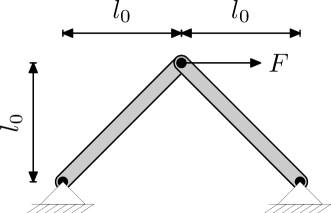
This first example consists of a simple plane truss under finite strain hypothesis. The structure consists of two connected bars of equal length $l_{0}=\sqrt{2}$ and section $A=10^{-2}$, pinned at their ends (see Fig. 2). The pinned nodes have Cartesian coordinates $\left(0.0,0.0\right)$ and $\left(2.0,0.0\right)$. In the central node, a horizontal force $F=5\cdot 10^{6}$ is applied. The material of the bars is elasto-plastic with Young’s modulus $E=210\cdot 10^{9}$, Poisson’s ratio $\nu=0.3$, a von Mises yield function with yield stress $\sigma_{e}=230\cdot 10^{6}$ and isotropic hardening modulus $H=4\cdot 10^{9}$. Since the deformation of the cross section is uniform, only one quadrature point is chosen on it to evaluate the section response.

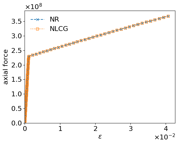
This simple problem allows to demonstrate the use of a non-linear conjugate gradient (NLCG) method to solve both the global problem and the local constitutive relations, and compare it with the solution obtained with a Newton-Raphson solver, both at the global and local levels. Figure 3 shows the axial force vs elongation, $\epsilon=\frac{l-l_{0}}{l_{0}}$, in the bar that is under tension. As expected, both methods give the same result, and we note that the NLCG never requires the computation of a tangent operator.

Figure 4: Geometry of beam problem.

5.2 Beam problem

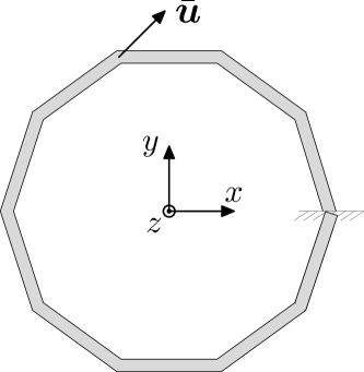
In the second example we study the response of a beam with the shape of a decagon, see Figure 4, under the small strain hypothesis. The beam axis lies in the $xy$-plane and the circumscribed circle radius is $r$. The cross section at one of the nodes is clamped. The cross section at the third vertex of the decagon, counting form the clamped one, is subject to an imposed displacement $\bm{u}=\delta(\bm{i}+\bm{j}+\bm{k})$, where the vectors $(\bm{i},\bm{j},\bm{k})$ refer to the canonical basis. The cross section of the beam is rectangular with sides $a$ and $b$. The side with dimension $a$ is parallel to the $xy$ plane, and the side with dimension $b$ is perpendicular to the first one and to the tangent direction of the beam. The material of the beam is elasto-plastic with Young’s modulus $E$, Poisson’s ratio $\nu$, a von Mises yield function of yield stress $\sigma_{e}$ and isotropic hardening modulus $H$. Under these conditions, the beam is subjected to axial, shear, bending, and torsion deformations.

Figure 5: Displacement in $x$ (left), $y$ (middle) and $z$ (right) for the beam problem at the end of the simulation.

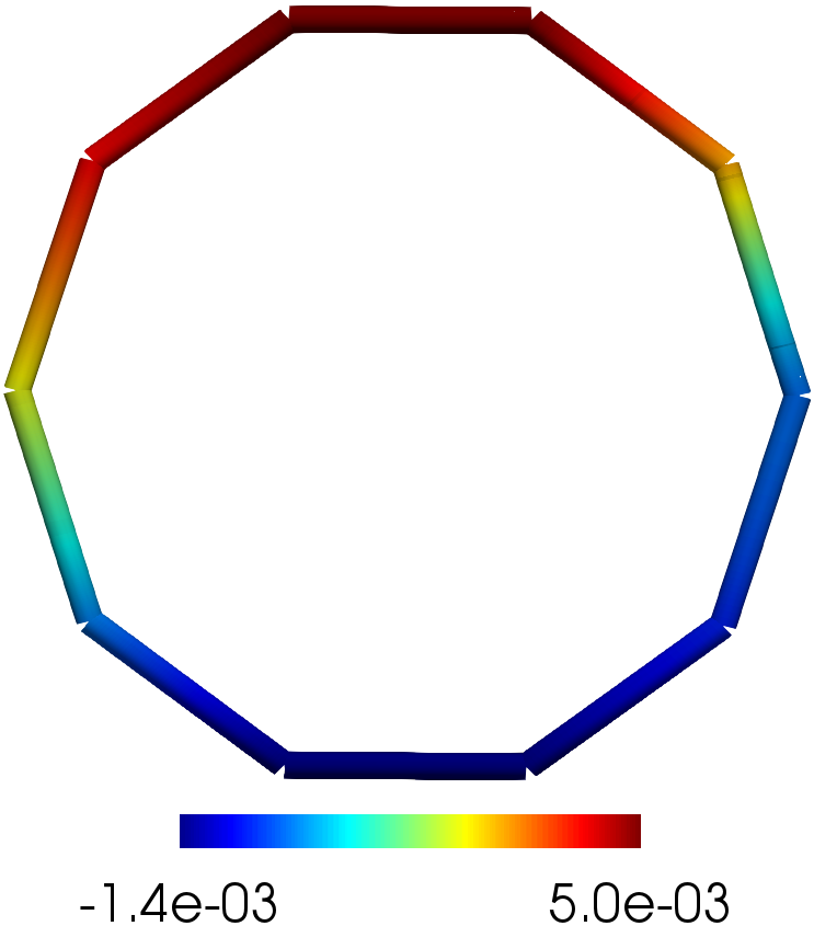
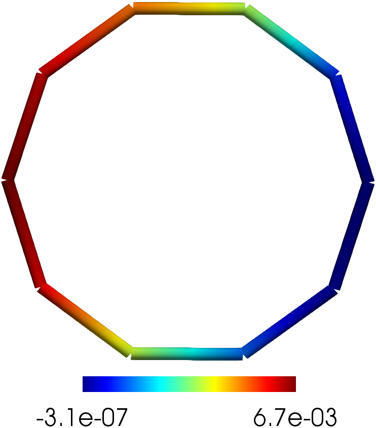
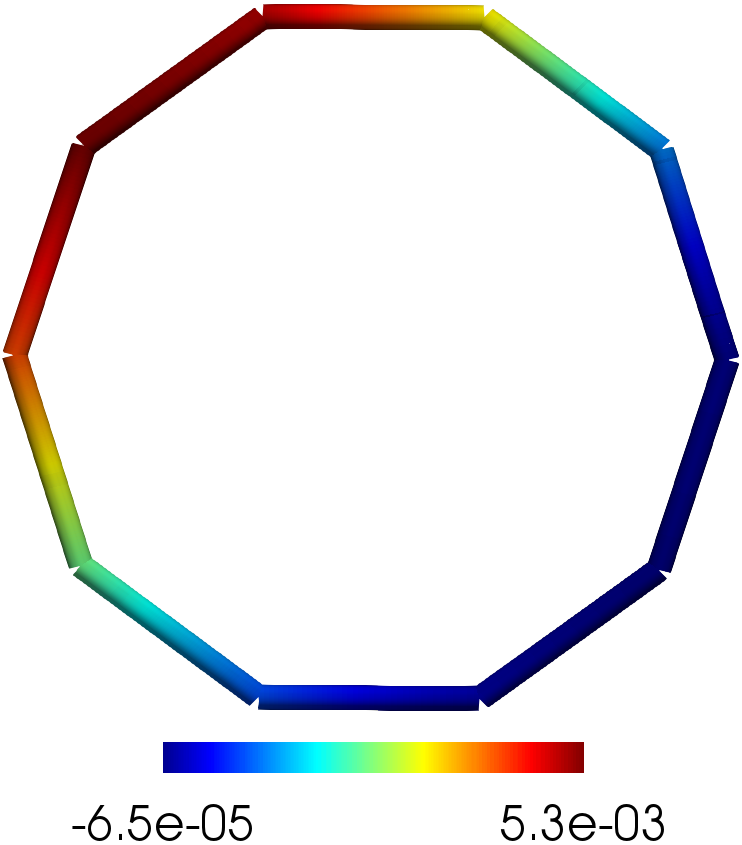
For the numerical example we select $r=0.5,\ \delta=5.0\cdot 10^{-3},\ E=210\cdot 10^{9},\ \nu=0.3,\ \sigma_{e}=200\cdot 10^{6},\ H=10\cdot 10^{9}$ and the beam is discretized with two-node elements with independent displacement and rotation interpolation, and selective reduced integration for the shear terms. An $8\times 8$ quadrature rule is chosen for the section constitutive response. Figure 5 shows the values of the displacements on the deformed shape of the beam when a mesh of 10 elements is employed.

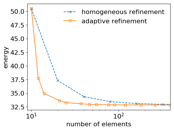
In order to improve the solution, we refine the mesh homogeneously. Figure 6 (left) shows the value of the global effective potential as a function of the number of elements in the mesh (in dashed blue line). As this number increases, the effective potential is reduced, converging to an asymptotic value, the “distance” to which can serve as an indicator of the accuracy of the solution.

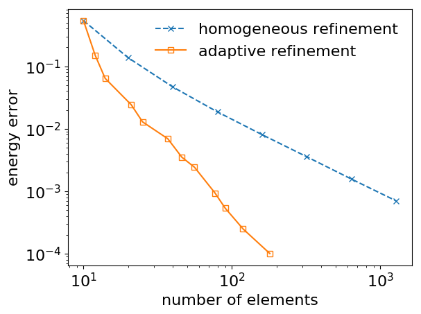
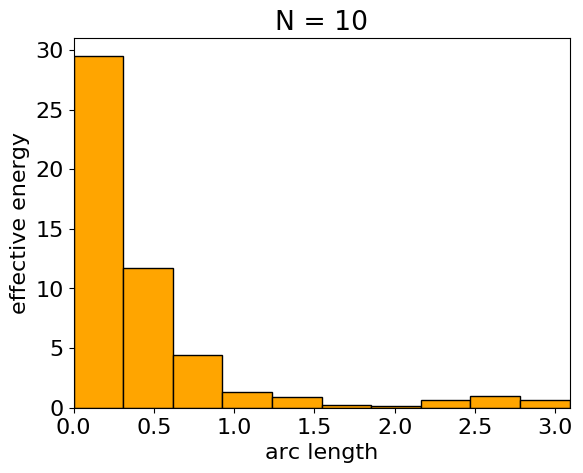
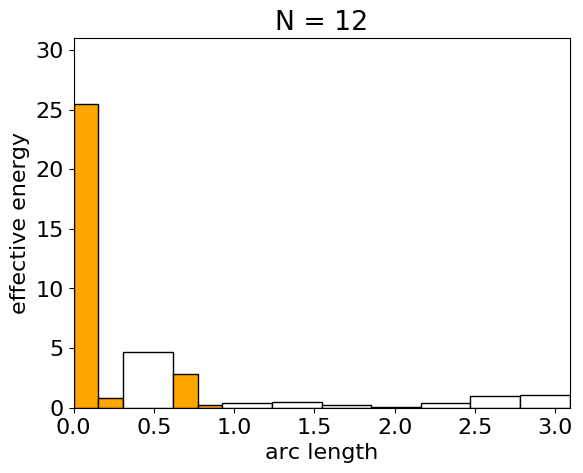
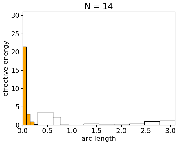
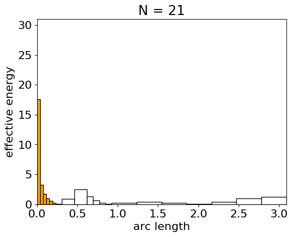
The local value of the effective potential can be used as an indicator for local mesh refinement. In a second solution, we proceed to refine the mesh by halving those beam elements that contribute most to the global value of the effective potential. For that, we proceed as in [14], studying the addition of a new node locally. For each element in the original mesh, we compare the energy obtained in the latest refinement with the one obtained in a local problem that results from halving the element and imposing the displacements and rotations of the latest calculation in the boundary nodes. Then, we subdivide the element if this energy difference is larger than the global average, hence searching for a more regular distribution of the effective potential energy density. Figure 6 (left) depicts the value of the total effective energy as a function of the number of elements refined in this anisotropic fashion (solid orange line). In Figure  6 (right) the relative energy error as a function of the number of elements for both refinement strategies is depicted. When compared with the homogeneous refinement, it follows that the locally refined mesh approximates faster the exact solution than the globally refined one. This, in turn, justifies the consideration of the effective potential energy as a valid error indicator. Figure 7 shows the efective potential energy per element in four consecutive local refinements, with the element size can be deduced from the abscissae.

Figure 6: Effective energy vs number of elements (left) and Relative energy error vs number of elements (right) for the homogeneous and adaptive mesh refinement strategies.

Figure 7: Effective energy of each element for four consecutive iterations of the adaptive refinement strategy. In orange, the elements with the smallest length. The total number of elements in the mesh is indicated above each plot.

5.3 Pinched cylinder

Figure 8: Pinched cylinder, left: problem setup, right: deformed structure in final stage with corresponding contour plot of displacement $v_{z}$.

Next we consider two shell problems. Both are solved using a primal isogeometric Kirchhoff-Love shell formulation with numerical integration through the shell’s thickness, as presented in [15]. The shell formulation employed uses stresses, rather than stress resultants, which is in contrast to most shell formulations found in literature. However, the resulting formulation provides practically identical results as the formulations presented in [16] and [17], where the initial isogeometric Kirchhoff-Love shell formulation [18], which was based analytical preintegration, was reformulated in terms of a numerical integration through the thickness of the shell body. All discretizations contain at least quadratic, $C^{1}$-continuous NURBS shape functions within a patch. In the shell’s in-plane directions, we use a “full” integration scheme with $p+1$ Gauss points, where $p$ is the polynomial degree of the shape functions. The number of integration points in the thickness direction is variable, but chosen to be equal to three for the presented examples.

As first shell problem, we study the pinching of a cylinder employing a hyperelastic material model, i. e. a compressible Neo-Hooke material with Young’s modulus of $E=168000\,\mathrm{N/mm}^{2}$ and Poisson’s ratio of $\nu=0.4$. The problem setup for a very thick (slenderness $R/t=4.5$) and a moderately thin cylinder (slenderness $R/t=45$) was first proposed by [19] and subsequently studied by variuos researchers, see for instance [20, 21]. All the articles mentioned consider three-dimensional or solid shell formulations making use of fully three-dimensional constitutive laws. Here, we only consider the thin case, since a thin shell formulation of Kirchhoff-Love type is used, as it was done in [16]. For the sake of comparability, we use a discretization of the shell problem in accordance with [16], i. e. we use a fourth order, $C^{3}$-continuous discretization with $32\times 12$ elements for modeling the whole cylinder, see Figure 8. In [16], one half of the cylinder was modeled with corresponding application of symmetry boundary conditions. With a slight difference, we instead model the whole cylinder with four patches consisting of $8\times 12$ elements each, coupled with the bending strip method from [22], where a penalty parameter has to be chosen.

The simulation is performed by controlling the vertical displacement $v_{z,A}$ at point $A$ in 16 steps of $\Delta v_{z,A}=-10\,\mathrm{mm}$. For the maximum displacement $v^{\text{max}}_{z,A}=-160\,\mathrm{mm}$ the resulting force $F^{\text{max}}$ is measured and compared to values obtained in literature. For penalty parameters of $10^{2}$ and $10^{3}$ we obtain the resulting forces $F^{\text{max}}=34.72\,\mathrm{kN}$ and $F^{\text{max}}=34.77\,\mathrm{kN}$, respectively. For higher penalty parameters the convergence properties get worse. In [16], a value of $F^{\text{max}}=34.86\,\mathrm{kN}$ was reported, whereas the results obtained with three-dimensional or solid shell formulations vary from $F^{\text{max}}=34.59\,\mathrm{kN}$ to $F^{\text{max}}=35.47\,\mathrm{kN}$, as reported in [21]. Our obtained results are consequently in good agreement with the results from the literature.

5.4 Simply supported plate

Figure 9: Simply supported plate, left: problem setup, right: deformed structure in final stage with corresponding contour plot of displacement $v_{z}$.

The second shell problem consists of a simply supported plate with a large strain plastic material, i. e. perfect $J_{2}$-plasticity with Young’s modulus $E=6.9\cdot 10^{4}\,\mathrm{N/mm}^{2}$, Poisson’s ratio $\nu=0.3$ and yield stress ${\sigma}_{y}=248\,\mathrm{N/mm}^{2}$. As shown in Figure 9, the quadratic plate has a side length of $L=508\,\mathrm{mm}$ and a thickness of $t=2.54\,\mathrm{mm}$, resulting in a slenderness ratio of $L/t=200$. All edges of the plate are simply supported in $z$-direction and the plate is subjected to a uniform dead load of $q_{z}=0.01\,\mathrm{N/mm}^{2}$ . The plate problem with this type of loading can be found in several references, see for instance [19, 23, 24, 25, 26, 21].

Figure 10: Simply supported plate, employed meshes with quadratic, $C^{1}$-continuous B-splines, left: $25\times 25$ elements, left: $31\times 31$ elements, right: $37\times 37$ elements, top: uniform meshes, bottom: nonuniform (NU) meshes.

Although symmetry may be taken into account, we model the whole plate structure and discretize it with six different, uniform and nonuniform (NU) refined meshes using quadratic, $C^{1}$-continuous B-splines. The meshes employed are shown in Figure 10 and consist of $25\times 25$, $31\times 31$, and $37\times 37$ elements, respectively. In all cases, three Gauss points through the thickness are used, since there is only a marginal change in the results when changing the number of Gauss points in the thickness direction, for example to five. This observation matches the one made in [21], where five Gauss points through the thickness have been used for a trilinear solid shell finite element, although the results did not sinificantly differ compared to the solution with two Gauss points in the shell’s thickness direction.

Figure 11: Simply supported plate, load-displacement diagram for different uniform and nonuniform (NU) meshes.

All simulations are performed with load control, using increments of different magnitude. We start with ten increments of $\Delta{\lambda}=0.2$, followed by ten increments of of $\Delta{\lambda}=0.8$. Between ${\lambda}=10$ and ${\lambda}=20$, we use 50 increments of $\Delta{\lambda}=0.2$, followed by 50 increments of $\Delta{\lambda}=0.8$, until the maximum load level of 50 increments of ${\lambda}=60$ is reached. More efficient time stepping schemes are not within the scope of this paper. The load-displacement curves obtained are plotted in Figure 11 and compared with the results obtained in [21] with a $64\times 64$ uniform finite element mesh. The uniform $25\times 25$ and $31\times 31$ meshes behave too stiff in a large portion of the load-displacment diagram, whereas the uniform $37\times 37$ element mesh is only slightly too stiff. The effective stored energy density distribution for the uniform $25\times 25$ mesh is shown in Figure 12 for two different load levels of ${\lambda}=10$ and ${\lambda}=20$. The plots directly suggest a mesh refinement in the corner regions, for which the three NU meshes try to account for.

Figure 12: Simply supported plate, effective stored energy density, integrated through the shell’s thickness, with unit of $\mathrm{kNm}/\mathrm{m}^{2}$ at different load levels for uniform $25\times 25$ element mesh, left: ${\lambda}=10$, right: ${\lambda}=20$.

The results for the $25\times 25$ NU and $31\times 31$ NU meshes are slightly too stiff towards the maximum load level, probably because of a too coarse mesh size at the tip of the plastic fold lines. The finest mesh with $37\times 37$ elements produces results in good agreement with the results obtained in [21]. The curves practically match each other, except of a slight difference in the region between approximately ${\lambda}=10$ to ${\lambda}=15$.

6 Summary and outlook

Structural models employing complex material models (inelastic, rate-dependent, etc.) require the solution of constrained three-dimensional material constitutive laws for the evaluation of their section response. This article starts by describing in an abstract way how these two problems are linked in an arbitrary structural model.

The main result of this work is the identification of a variational setting behind the problem of general structural models, encompassing three-dimensional laws, both elastic and inelastic. Starting from a new result that identifies the minimization problem behind every constrained three-dimensional constitutive relation, and based on the abstract framework described first, we have revealed that there is a single optimization program to be solved when analyzing general structural models with complex materials.

This result has several consequences: from the theoretical point of view it sets the stage for fundamental analyses including the existence of solutions, an aspect that is beyond this work’s goals. From the computational side, it guarantees the symmetry of the Hessian and points towards (descend) iterative methods for the solution of these problems that have not been identified previously in the literature. Furthermore, the effective potential that is the basis for the solution provides an intrinsic error indicator for a general class of structural models, including geometric and material nonlinearities. This is a remarkable result, and the first of its class to the authors’ knowledge, illustrating how the variational framework bridges the mechanics of three-dimensional and reduced models.

Numerical methods, implemented in a publicly available library of material models, show the validity of the approach and illustrate the possibilities of mesh adaptation based on the new error indicator.

References

- [1] E P Popov. Introduction to mechanics of solids. Prentice-Hall, Englewood Cliffs, New Jersey, 1968.
- [2] S Timoshenko and J M Gere. Mechanics of materials. Van Nostrand Reinhold, New York, first ed. edition, 1972.
- [3] S Govindjee. Engineering Mechanics of Deformable Solids. A Presentation with Exercises. Oxford University Press, October 2012.
- [4] R de Borst. The zero-normal-stress condition in plane-stress and shell elastoplasticity. Communications in Applied Numerical Methods, 7:29–33, 1991.
- [5] S. Klinkel and S. Govindjee. Using finite strain 3d-material models in beam and shell elements. Engineering Computations, 19(3):254–271, 2002.
- [6] Nunziante Valoroso and Luciano Rosati. Consistent derivation of the constitutive algorithm for plane stress isotropic plasticity. Part II: Computational issues. International Journal of Solids and Structures, 46(1):92–124, 2009.
- [7] E A de Souza Neto, D Peric, and D R J Owen. Computational Methods for Plasticity. Theory and Applications. John Wiley & Sons, Chichester, UK, 2008.
- [8] M. Ortiz and L Stainier. The variational formulation of viscoplastic constitutive updates. Computer Methods in Applied Mechanics and Engineering, 171(3):419–444, 1999.
- [9] D. Portillo, D. del Pozo, D. Rodríguez-Galán, J. Segurado, and I. Romero. MUESLI - a Material UnivErSal LIbrary. Advances in Engineering Software, 105:1–8, 2017.
- [10] M Epstein. The geometric language of continuum mechanics. Cambridge University Press, Cambridge, 2010.
- [11] R Radovitzky and M. Ortiz. Error estimation and adaptive meshing in strongly nonlinear dynamic problems. Computer Methods in Applied Mechanics and Engineering, 172(1):203–240, April 1999.
- [12] C Miehe, J Schotte, and M Lambrecht. Homogenization of inelastic solid materials at finite strains based on incremental minimization principles. Application to the texture analysis of polycrystals. Journal of the Mechanics and Physics of Solids, 50(10):2123–2167, 2002.
- [13] J Mosler and O T Bruhns. On the implementation of rate-independent standard dissipative solids at finite strain–Variational constitutive updates. Computer Methods in Applied Mechanics and Engineering, 199:417–429, 2010.
- [14] J Mosler and M Ortiz. Variational h-adaption in finite deformation elasticity and plasticity. International Journal for Numerical Methods in Engineering, 72:505–523, 2007.
- [15] Bastian Oesterle, Renate Sachse, Ekkehard Ramm, and Manfred Bischoff. Hierarchic Isogeometric Large Rotation Shell Elements Including Linearized Transverse Shear Parametrization. Computer Methods in Applied Mechanics and Engineering, 321:383–405, 2017.
- [16] J. Kiendl, M.-C. Hsu, M. C. H. Wu, and A. Reali. Isogeometric Kirchhoff–Love shell formulations for general hyperelastic materials. Computer Methods in Applied Mechanics and Engineering, 291:280–303, 2015.
- [17] Marreddy Ambati, Josef Kiendl, and Laura De Lorenzis. Isogeometric Kirchhoff-Love shell formulation for elasto-plasticity. Computer Methods in Applied Mechanics and Engineering, 340:320–339, 2018.
- [18] J. Kiendl, K. U. Bletzinger, J. Linhard, and R. Wüchner. Isogeometric shell analysis with Kirchhoff–Love elements. Computer Methods in Applied Mechanics and Engineering, 198(49–52):3902–3914, 2009.
- [19] Norbert Büchter, Ekkehard Ramm, and Deane Roehl. Three-Dimensional Extension of Non-Linear Shell Formulation Based on the Enhanced Assumed Strain Concept. International Journal for Numerical Methods in Engineering, 37(15):2551–2568, 1994.
- [20] Boštjan Brank, Jože Korelc, and Adnan Ibrahimbegović. Nonlinear shell problem formulation accounting for through-the-thickness stretching and its finite element implementation. Computers & Structures, 80(9):699–717, 2002.
- [21] Marco Schwarze and Stefanie Reese. A Reduced Integration Solid-Shell Finite Element Based on the EAS and the ANS Concept–Large Deformation Problems. International Journal for Numerical Methods in Engineering, 85(3):289–329, 2011.
- [22] J. Kiendl, Y. Bazilevs, M. C. Hsu, R. Wüchner, and K. U. Bletzinger. The bending strip method for isogeometric analysis of Kirchhoff–Love shell structures comprised of multiple patches. Computer Methods in Applied Mechanics and Engineering, 199(37–40):2403–2416, 2010.
- [23] Christian Miehe. A theoretical and computational model for isotropic elastoplastic stress analysis in shells at large strains. Computer Methods in Applied Mechanics and Engineering, 155(3):193–233, 1998.
- [24] R. Hauptmann, S. Doll, M. Harnau, and K. Schweizerhof. ‘Solid-shell’ elements with linear and quadratic shape functions at large deformations with nearly incompressible materials. Computers & Structures, 79(18):1671–1685, 2001.
- [25] Stefanie Reese. A large deformation solid-shell concept based on reduced integration with hourglass stabilization. International Journal for Numerical Methods in Engineering, 69(8):1671–1716, 2007.
- [26] Sven Klinkel, Friedrich Gruttmann, and Werner Wagner. A mixed shell formulation accounting for thickness strains and finite strain 3d material models. International Journal for Numerical Methods in Engineering, 74(6):945–970, 2008.