Topological Constraints in the Reconnection of Vortex Braids

Abstract

We study the relaxation of a topologically non-trivial vortex braid with zero net helicity in a barotropic fluid. The aim is to investigate the extent to which the topology of the vorticity field – characterized by braided vorticity field lines – determines the dynamics, particularly the asymptotic behaviour under vortex reconnection in an evolution at high Reynolds numbers ($25,000$). Analogous to the evolution of braided magnetic fields in plasma, we find that the relaxation of our vortex braid leads to a simplification of the topology into large-scale regions of opposite swirl, consistent with an inverse cascade of the helicity. The change of topology is facilitated by a cascade of vortex reconnection events. During this process the existence of regions of positive and negative kinetic helicity imposes a lower bound for the kinetic energy. For the enstrophy we derive analytically a lower bound given by the presence of unsigned kinetic helicity, which we confirm in our numerical experiments.

I Introduction

It is well established that the degree of tangling/knottedness of vorticity field lines can have important implications for the dynamics of a fluid (Moffatt, 1969, 1992). In a barotropic fluid in the ideal case with zero viscosity this tangling is preserved, restricting the lowest energy state to which the fluid has access. This has been demonstrated both in experiments (Scheeler et al., 2014, 2017) and numerical simulations (Kerr, 2018). When the Reynolds number is large but finite, vortex reconnection may take place, permitting a change of topology of the vortex lines. Individual events of such vortex reconnection have been studied, typically involving reconnection between isolated vortex tubes or rings (Ashurst and Meiron, 1987; Melander and Hussain, 1989; Kida, Takaoka, and Hussain, 1991; van Rees, Hussain, and Koumoutsakos, 2012; McGavin and Pontin, 2018; Zhao et al., 2021). Notably, in these simulations the vortex tubes usually contort during their mutual approach, such that the vortex lines reconnect locally anti-parallel (in a 2d plane). However, in many applications, the vorticity is a smooth non-vanishing function across the volume and can’t be modelled as a set of interacting isolated tubes. Examples include rotating stars and planets where there is a dominant direction of the vorticity (aligned with the rotation axis) onto which contributions from convection are superimposed. The resulting field could be interpreted as a vortex braid. If vortex reconnection occurs in such a scenario, the presence of a dominant uni-directional vorticity field means that the reconnection is fully three-dimensional (Hornig, 2001), as recently observed in the reconnection of vortex tubes with swirl (van Rees, Hussain, and Koumoutsakos, 2012; McGavin and Pontin, 2019). Note that with “vortex reconnection” here we refer to the process by which the vorticity field lines change their topology, prohibited in a barotropic, inviscid fluid. This should not be confused with the notion of reconnection of vorticity isosurfaces, also sometimes referred to as vortex reconnection.

We analyze in the following the relaxation of a braided vorticity field in a fluid of high Reynolds number ($\mbox{\rm Re}>10^{4}$). The aim is to investigate the extent to which the topology of the vorticity field – characterized by braided vorticity field lines – determines the dynamics. With the notion “braided” we describe a situation where we have a dominant component of the vorticity field in one direction, in our case the $z$-direction, so that all vorticity field lines connect two opposite sides of our domain (see Figure 1). The motivation for this scenario is three-fold: First, the situation of a braided vorticity field is of relevance for many cases of rotating astrophysical bodies, where the rotation of the star or planet provides a dominant component of the vorticity and the contributions from convection or turbulence to the vorticity are weaker and only contribute to a braiding of the vortex lines. Second, this set-up has the advantage that all vorticity lines connect from the lower to upper boundary of our domain. That is, there are no null points of the vorticity in the domain and hence the topological structure of the field is uniquely described by its vorticity-field line mapping from the lower to the upper boundary (Yeates and Hornig, 2013). This allows us to analyze the topology of the field at any point in time using various tools such as the field line helicity (Yeates and Hornig, 2011a, 2013), the topological entropy (Candelaresi, Pontin, and Hornig, 2017), or the topological degree (Yeates, Hornig, and Wilmot-Smith, 2010). With these tools one can follow the dynamics of the relaxation with the ultimate aim to make predictions regarding the final state of the relaxation process. One can even identify individual processes of vortex reconnection taking place. However, in this study we are less interested in the individual reconnection events and more in the collective effect that a turbulent cascade of reconnection events has on the route the relaxation process takes. The third motivation is that this vortex braid relaxation is the exact analogue to a magnetic braid relaxation studied by the authors before (Wilmot-Smith, Hornig, and Pontin, 2009). In these previous studies the relaxation exhibited additional constraints on the dynamics, over and above the one imposed by the conservation of helicity Yeates, Hornig, and Wilmot-Smith (2010). To investigate the presence of such constraints in vortex dynamics is the aim of this study.

II Model

II.1 Initial Condition

We wish to construct a vortex braid in which all vorticity field lines connect between opposite boundaries of the domain. In order to facilitate direct comparison with a well-studied magnetic braid we choose the particular braiding pattern of the vorticity lines to be analogous to that of the magnetic field lines in that magnetic braid (Wilmot-Smith, Hornig, and Pontin, 2009). The vorticity field consists of a constant background field in the $z$-direction together with two vortex rings with their symmetry axes also aligned to the $z$-direction. The vortex rings are located such that we obtain vorticity field lines as in Figure 1 (see also Figure 8). All vorticity lines connect between opposite (plane-parallel, constant-$z$) boundaries. The background vorticity field is conveniently obtained from a (solid-body) rotational flow with the $z$-axis as the axis of rotation. An illustration is shown in Figure 1, which corresponds to the vortex field we will be using.

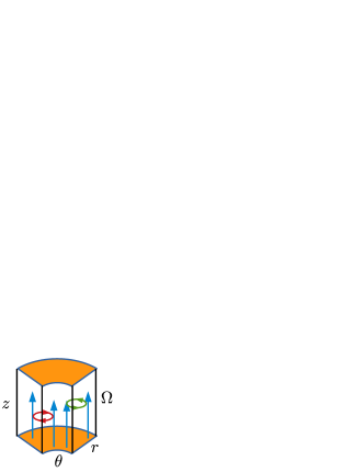
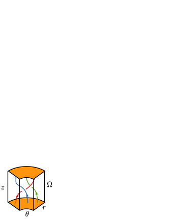
Figure 1: Schematic representation of the initial set up of the vortex braid. Left we represent the components of the field with the two vortex rings (red and green) of opposing vorticity sign and the background vorticity (blue). On the Right we show the superposition of the vortex rings with the background field which results in the vortex braid.

To avoid complications of generation of secondary vortices in domain corners, something that typically occurs in Cartesian geometries for rotating fluids, we make use of a cylindrical domain, which rotates about the $z$-axis. We construct the field first without the homogeneous background in a cylindrical wedge with periodic azimuthal boundaries and move the frame of reference together with the global rotational flow. To obtain the effect of the background field (and the full vortex braid) we add a Coriolis term in the momentum equations (see below).

Each of the vortex rings (red and green in Figure 1) is constructed by first defining a single vortex ring centered at the origin. This greatly simplifies our calculations, due to the ring’s azimuthal symmetry. We then translate the calculated field to its position in the wedge domain; a non-trivial transformation, as described in Appendix A.

For our computational domain we choose a cylindrical wedge of dimensions $r\in[45,65]$, $\theta\in[-0.1,0.1]$ and $z\in[-16,16]$. We choose the $\theta$ and $z$ directions to be periodic, while the boundary conditions in the radial direction are chosen such that the normal component of the velocity vanishes and any mass flux is suppressed.

Within this domain we place two vortex rings of opposite orientation, with axes lying in planes of constant $z$ and centers at positions $(r,\theta,z)=(55,\arctan{(1/55)},-8)$ and $(r,\theta,z)=(55,-\arctan{(1/55)},8)$. This means that the subsection of our volume in which the vortex lines exhibit a non-trivial tangling is located centrally within the domain, away from the $r$ and $\theta$ boundaries. The initial vertical distance of 16 in non-dimensional code units between the (axes of the) vortex rings ensures that the velocities induced by the two vortex rings do not significantly overlap at $t=0$. Note that the superposition of the vortex ring with the background vorticity leads to a local twisting of the vorticity lines, and since the boundaries are periodic along $z$, the vorticity lines in principle pass through infinitely many of these vortex rings.

To prevent effects from supersonic flows we choose the amplitude of the vorticity in the vortex rings to $\alpha=0.1$. This will keep the velocities throughout the simulations well below the sound speed of $1$. For the background vorticity we choose $\bm{\Omega}=0.1\mbox{\boldmath$e$}{}_{z}$. This will lead to a vorticity field with the desired topology. The ratio of the two amplitudes $\alpha/\Omega$ determines the strength of the braiding and with that the topology of the vortex field. Note that this constant background vorticity refers to the rest frame, and is achieved by using a Coriolis term in the simulations with the angular velocity $\tilde{\bm{\Omega}}=\bm{\Omega}/2$.

With these parameters we obtain a Rossby number

$$\mbox{\rm Ro}=\frac{u}{2L\tilde{\Omega}},$$ (1)

where $u$ is a typical velocity and $L$ a typical length scale. In our case $u\approx 0.1$ (velocity at the vortex rings), $L\approx 1$ (size of the vortex rings) and $\tilde{\Omega}=0.05$. With that we have $\mbox{\rm Ro}\approx 1$.

II.2 Numerical Setup

As described above, to circumvent issues at the domain’s corners and issues with non-vanishing normal velocities at the boundaries, we place our cylindrical wedge domain in a co-moving frame. This generates the additional term of the Coriolis force $2\mbox{\boldmath$u$}{}\times\tilde{\bm{\Omega}}$. Our resulting equations are then the equations of motion for a viscous, isothermal and compressible gas:

$$\frac{{\rm D}{}\mbox{\boldmath$u$}{}}{{\rm D}{}t}=-c_{\rm s}^{2}\mbox{\boldmath$\nabla$}{}\ln{\rho}+2\mbox{\boldmath$u$}{}\times\tilde{\bm{\Omega}}+\mbox{\boldmath$F$}{}_{\rm visc},$$ (2)

$$\frac{{\rm D}{}\ln{\rho}}{{\rm D}{}t}=-\mbox{\boldmath$\nabla$}{}\cdot\mbox{\boldmath$u$}{},$$ (3)

with the isothermal speed of sound $c_{\rm s}$, density $\rho$, viscous forces $\mbox{\boldmath$F$}{}_{\rm visc}$ and Lagrangian time derivative ${\rm D}{}/{\rm D}{}t=\partial/\partial t+\mbox{\boldmath$u$}{}\cdot\mbox{\boldmath$\nabla$}{}$. Here the viscous forces are given as $\mbox{\boldmath$F$}{}_{\rm visc}=\rho^{-1}\mbox{\boldmath$\nabla$}{}\cdot 2\nu\rho\mbox{\boldmath$S$}{}$, with the kinematic viscosity $\nu$, and traceless rate of strain tensor $\mbox{\boldmath$S$}{}_{ij}=\frac{1}{2}(u_{i,j}+u_{j,i})-\frac{1}{3}\delta_{ij}\mbox{\boldmath$\nabla$}{}\cdot\mbox{\boldmath$u$}{}$. Being an isothermal gas we have $p=c_{\rm s}^{2}\rho$ for the pressure. Note that since $c_{\rm s}^{2}$ is constant, $\nabla p\times\nabla\rho=0$, meaning that there is no baroclinic vorticity production.

Equations (2)–(3) are solved using the PencilCode , which is an Eulerian finite-difference code using sixth-order spatial derivatives and a third-order time-stepping scheme (Brandenburg and Dobler, 2002). Throughout our simulations we use $\nu=10^{-3}$ to $\nu=4\times 10^{-5}$ in order to reduce kinetic energy dissipation and kinetic helicity dissipation as much as the limited resolution of $512\times 256\times 256$ ($r$, $\theta$, $z$) grid points allows. We emphasize that due to the barotropic nature of the fluid, in the inviscid case the tangling (or braiding) of the vortex lines would be preserved for all time.

II.3 Incompressibility

By construction the initial velocity field has the property $\mbox{\boldmath$\nabla$}{}\cdot\mbox{\boldmath$u$}{}\approx 0$. Being approximately incompressible, any calculations involving the evolution of the kinetic energy or enstrophy significantly simplify. This implies that the initial uniform density does not change in time (see equation (3)). However, numerical errors in the calculation of the potential $C_{0}$ (equation (17)) can cause deviations from $\mbox{\boldmath$\nabla$}{}\cdot\mbox{\boldmath$u$}{}=0$.

To check if our assumption of incompressibility holds true for all time we plot the maximum and minimum density in the domain as a function of time (Figure 2). We observe a deviation of ca. $0.5$% from the uniform density at initial time, which quickly decreases to ca. $0.2$% and approximately remains constant. Being such a small deviation we can safely assume that the system is approximately incompressible.

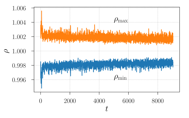
Figure 2: Minimum and maximum density in the domain as a function of time for the simulation with viscosity $\nu=4\times 10^{-5}$.

III Evolution of the System

Following initiation of the simulation, the two vortex rings travel towards one another due to their self-induced motion, meeting approximately at the mid-plane, $z=0$. This is analogous to the self-induced motion of an isolated infinitesimal vortex ring (i.e. with infinitesimal minor radius), with some distortion due to the presence of the background vorticity and the finite radius of the rings. Due to the offset in $\theta$ between the two rings, they do not meet face-on (Figure 3). However, their collision leads to a local enhancement of the vorticity where they meet, as seen in the enstrophy evolution (see section IV).

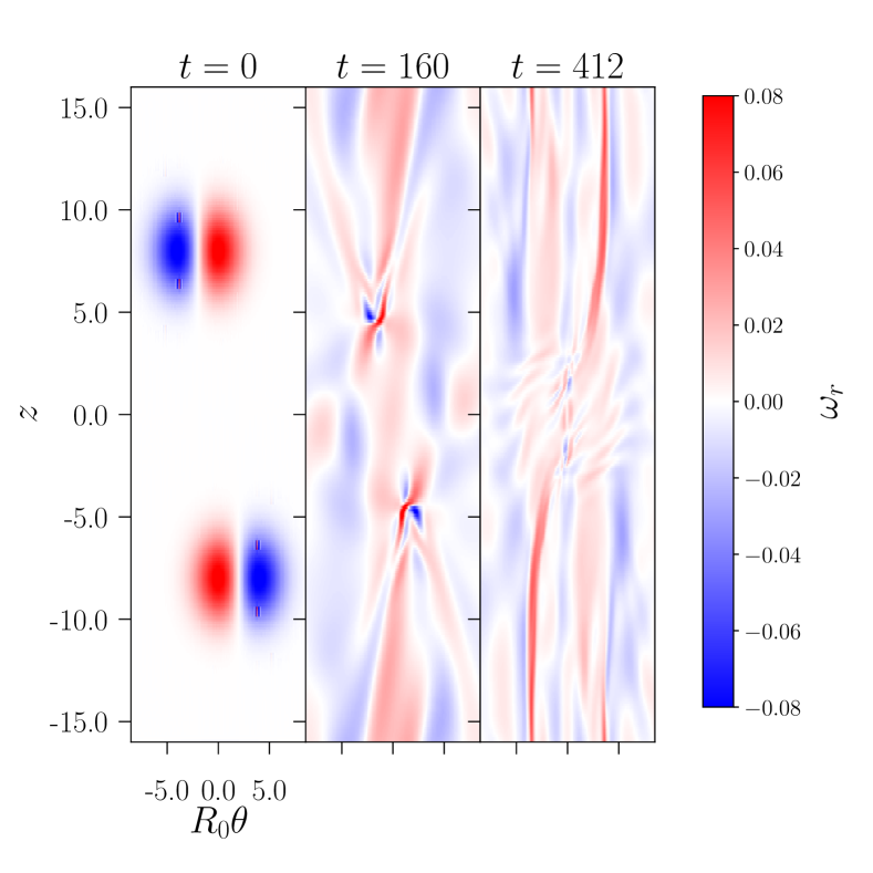
Figure 3: Slices through the domain for $\omega_{r}$ at different times at $r=R_{0}=55$ for the simulation with viscosity $\nu=4\times 10^{-5}$.

From previous studies of the relaxation of magnetic braids we know that the braid constructed in this way requires many reconnection events to untangle and is very efficient in generating a turbulent evolution. Following the initial collision, we see indeed that a highly-fluctuating, “turbulent-like” evolution ensues, in which we find numerous locations at which vortex reconnection takes place (identified by calculating $(\nabla\times\mbox{\boldmath$\omega$}{})\cdot(\mbox{\boldmath$\omega$}{}+\bm{\Omega})/|\mbox{\boldmath$\omega$}{}+\bm{\Omega}|$, see (Hornig, 2001; McGavin and Pontin, 2018)). Through these many localized reconnection events the field topology simplifies, with the vortex lines becoming less tangled. However, the final state retains a non-trivial topology, and our main purpose is to analyse the way in which this final state is determined by the initial field topology.

IV Enstrophy

Unlike the total energy and the kinetic helicity, the enstrophy

$$\mathcal{E}=\int_{V}\mbox{\boldmath$\omega$}{}^{2}\ {\rm d}{}V$$ (4)

is not necessarily conserved, even in the inviscid case. To see the factors that can lead to a change in enstrophy, we use the momentum equation (2) to write the vorticity equation as

$$\frac{\partial\mbox{\boldmath$\omega$}{}}{\partial t} = \mbox{\boldmath$\nabla$}{}\times(\mbox{\boldmath$u$}{}\times\mbox{\boldmath$\omega$}{})+2\mbox{\boldmath$\nabla$}{}\times(\mbox{\boldmath$u$}{}\times\tilde{\bm{\Omega}})+\nu\Delta\mbox{\boldmath$\omega$}{}$$ (5)

$$+2\nu\mbox{\boldmath$\nabla$}{}\times(\mbox{\boldmath$\nabla$}{}\ln(\rho)\cdot\mbox{\boldmath$S$}{}).$$

With this we can write the time evolution of the total enstrophy as

$$\frac{{\rm d}{}\mathcal{E}}{{\rm d}{}t} = 2\int_{V}\mbox{\boldmath$\omega$}{}\cdot\frac{\partial\mbox{\boldmath$\omega$}{}}{\partial t}\ {\rm d}{}V$$ (6)

$$= 2\int_{\partial V}((\mbox{\boldmath$u$}{}\cdot\mbox{\boldmath$\omega$}{})\mbox{\boldmath$\omega$}{}+\nu\mbox{\boldmath$\omega$}{}\times\mbox{\boldmath$\nabla$}{}\times\mbox{\boldmath$\omega$}{})\cdot{\rm d}{}\mbox{\boldmath$S$}{}$$

$$+2\int_{V}\left((\mbox{\boldmath$u$}{}\times(\mbox{\boldmath$\omega$}{}+2\tilde{\bm{\Omega}}))\cdot\mbox{\boldmath$\nabla$}{}\times\mbox{\boldmath$\omega$}{}-\nu(\mbox{\boldmath$\nabla$}{}\times\mbox{\boldmath$\omega$}{})^{2}\right.$$

$$\left.+2\nu\mbox{\boldmath$\omega$}{}\cdot\mbox{\boldmath$\nabla$}{}\times(\mbox{\boldmath$\nabla$}{}\ln(\rho)\cdot\mbox{\boldmath$S$}{})\right)\ {\rm d}{}V,$$

where we used the fact that the azimuthal and vertical dimensions are periodic, $\mbox{\boldmath$u$}{}\cdot\mbox{\boldmath$n$}{}=0$ at the $r$ boundaries and $\tilde{\bm{\Omega}}\cdot\mbox{\boldmath$n$}{}=0$ on the $r$ and $\theta$ boundaries.

Apart from the terms involving viscosity, we have two more volume terms and one surface term that in general do not vanish. This is interesting, since our domain is closed in the radial direction and yet, there can be enstrophy fluxes through those boundaries. However, throughout all of our simulations the velocities near the radial boundaries are very small and this term can be safely ignored. The first volume term describes the dynamical generation or annihilation of enstrophy according to the alignment of the velocity, vorticity and its curl, while the second volume term describes the dynamical generation/annihilation of enstrophy due to the Coriolis force.

For high Reynolds numbers we observe first an increase and then a gradual decrease in enstrophy (Figure 4). As the vortex rings approach and collide, a large amount of vorticity is produced on small scales. Since this is a turbulent effect, it increases as we increase the Reynolds number. Indeed, the breakup of vortex sheets formed during vortex tube/ring collision is well documented (van Rees, Hussain, and Koumoutsakos, 2012; Kerr, 2013; McKeown et al., 2018). For higher Reynolds numbers the flow becomes more turbulent and the non-viscous terms in equation (6) become more dominant. It appears that the alignment of the fields is such that a net production of enstrophy is obtained. In numerical vortex reconnection experiments Yao and Hussain (2020); Nguyen and Duong (2021) showed a similar behavior of enstrophy production during reconnection events. With increasing Reynolds number, they too observe an increased enstrophy production. The Coriolis contribution to the enstrophy evolution seems to dampen the production through the term $(\mbox{\boldmath$u$}{}\times\mbox{\boldmath$\omega$}{})\cdot\mbox{\boldmath$\nabla$}{}\times\mbox{\boldmath$\omega$}{}$.

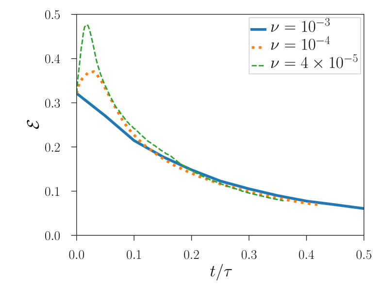
Figure 4: Enstrophy evolution for different viscosities $\nu$ against normalized (diffusion) time (see equation (8)).

V Kinetic Helicity

In the inviscid case the kinetic helicity (hereafter, simply “helicity”) is conserved. For a non-vanishing viscosity this will not be the case anymore. However, for the present configuration, due to the symmetry of the configuration, consisting of a vortex ring with positive and one with negative helicity, the volume-integrated helicity is zero and stays zero at all times. Nevertheless, the existence of helicity in parts of the domain can influence the relaxation. Indeed, it has been shown that in the relaxation of magnetic braids, not only the net helicity is important in constraining the dynamics, but also properties of the field line mapping as well as the helicity-per-fieldline spectrum (Pontin et al., 2011; Yeates, Hornig, and Wilmot-Smith, 2010; Yeates, Russell, and Hornig, 2015). A way to detect the existence of a non-vanishing helicity density in the domain is to track the evolution of the unsigned kinetic helicity as the integral over the magnitude of the helicity density

$$\bar{H}_{\rm kin}=\int_{V}|(\mbox{\boldmath$\omega$}{}+\bm{\Omega})\cdot(\mbox{\boldmath$u$}{}+\mbox{\boldmath$U$}{})|\ {\rm d}{}V,$$ (7)

where $\mbox{\boldmath$\nabla$}{}\times\mbox{\boldmath$U$}{}=\bm{\Omega}$. Note that here we include the background vorticity and velocity, that is we calculate the helicity in an inertial frame rather than the co-rotating frame. This is for two reasons. First, helicity conservation holds for the inertial frame but not in general for an accelerated frame. Second, only in the inertial frame do we have properly braided vorticity lines in the initial state, while in the corotating frame the kinetic helicity density vanishes everywhere at $t=0$.

Furthermore, one has to note that unsigned kinetic helicity is not conserved, even under conditions where the usual kinetic helicity is conserved. For instance, if an initially straight untwisted vortex tube fixed between two parallel plates is deformed by a rotation in the middle then the helicity is conserved as the left and right hand twist in the tube cancel, but the unsigned helicity increases. Nevertheless the unsigned helicity is always positive and can vanish only if the helicity density vanishes everywhere in the domain. The latter property is important for what follows, as it captures any non-zero helicity density in the domain.

We have run our simulations for different values of Re, and it is instructive to plot the results using time units that are normalized by the viscous dissipation time scale

$$\tau\approx L^{2}/\nu,$$ (8)

where $L$ is a typical length. Here we take $L$ to be the (major) radius of the vortex rings which is approximately $1$.

For our simulations we observe first a steep rise of $\bar{H}_{\rm kin}$ and then dissipation. Since for $\nu=10^{-3}$ we have $\tau=1000$ this means that by time $1000$ we should observe a significant decrease in kinetic helicity. Indeed, at time $t/\tau=0.5$ we observe a drop by a factor of $e^{-0.5}$ compared to its peak value at early times (Figure 5).

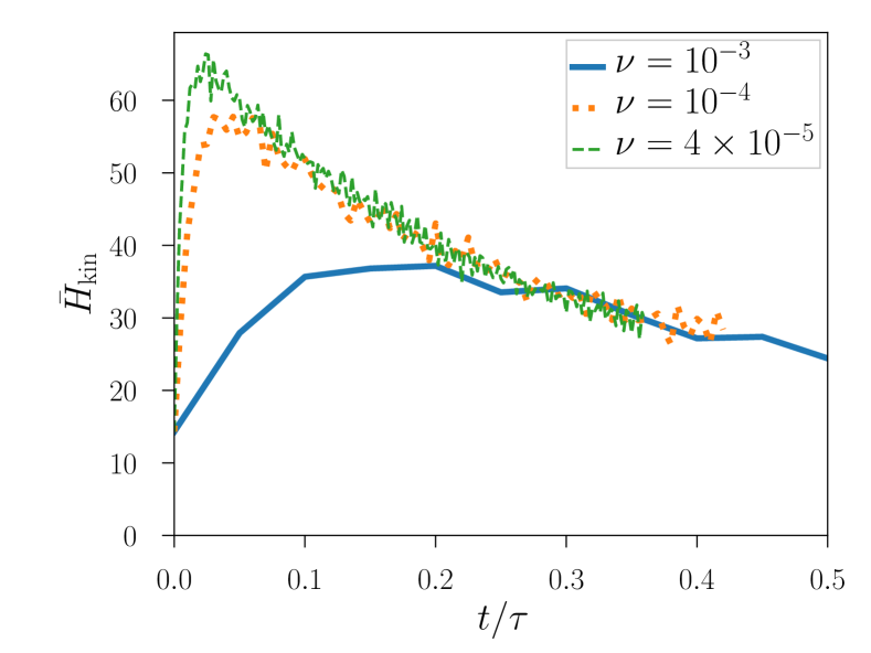
Figure 5: Evolution of the unsigned kinetic helicity for the relaxing vortex braid for different viscosities $\nu$ against normalized time (see equation (8)).

The initial rise happens at approximately $100$ code time units, independent of the viscosity, which means that it is a non-viscous effect. As the two initial vortex rings approach we observe an increase in kinetic helicity density until the time of collision, which is approximately $100$ code time units. This we attribute to vortex stretching. After that we observe that the viscosity takes over and dissipates $\bar{H}_{\rm kin}$. Note that for $\nu=10^{-3}$, 100 code time units corresponds to $t/\tau=0.1$, while for $\nu=10^{-4}$ the collision time is $t/\tau=0.01$ in normalized times.

V.1 Kinetic Helicity and Enstrophy

The motivation to consider the relation between helicity and enstrophy comes from the magnetic case where we know that the magnetic energy is limited from below by the magnetic helicity. This is known as the realizability condition, (Arnold, 1986; Brandenburg, Dobler, and Subramanian, 2002; Del Sordo, Candelaresi, and Brandenburg, 2010; Candelaresi and Brandenburg, 2011).

$$\left|H_{\rm mag}\right|\leq\frac{2}{\lambda}E_{\rm mag},$$ (9)

where $\lambda$ is the smallest positive eigenvalue of the curl operator in the domain Arnold (1986); Arnold and Khesin (2013). The inequality is sharp, that is there exist fields for which the equality holds and these are the eigenfields of the curl operator for the minimal eigenvalue $\pm\lambda$. The corresponding condition for vorticity fields would involve the enstrophy in the rest frame ${\cal E}^{\rm tot}$ and not the energy:

$$\left|H_{\rm kin}\right|\leq\frac{1}{\lambda}{\cal E}^{\rm tot}.$$ (10)

Since the helicity is defined in the rest frame we also have to use the definition of the enstrophy in the rest frame:

$${\cal E}^{\rm tot}=\int_{V}(\mbox{\boldmath$\omega$}{}+\bm{\Omega})^{2}\ {\rm d}{}V.$$ (11)

In our case this inequality is not very useful since $H=0$, which does not pose any lower bound on the enstrophy. However, as shown in the Appendix (B) we can find an even stronger inequality:

$$\bar{H}_{\rm kin} \leq \frac{1}{\lambda}\mathcal{E}^{\rm tot}$$ (12)

$$\Leftrightarrow\lambda \leq \frac{\mathcal{E}^{\rm tot}}{\bar{H}_{\rm kin}}$$ (13)

The minimal $\lambda$ is not easy to determine for our domain, but one can approximate by using the known minimal $\lambda=(2.405..)/R$ for a cylinder. The largest cylinder we can fit into our domain has $R=5$, hence the $\lambda$ for our domain should be roughly 0.48. The ratio $\mathcal{E}^{\rm tot}/\bar{H}_{\rm kin}$ is shown in Figure 6 and we clearly see that the enstrophy is bounded from below by the unsigned kinetic helicity with a ratio $\geq 1$.

For the curve with the highest viscosity we find after the initial relaxation an increase of the ratio $\mathcal{E}^{\rm tot}/\bar{H}_{\rm kin}$. This is a result of our particular set-up. As the viscous dissipation does not act on the fixed background vorticity field, the evolution will eventually dissipate everything but the background field and for the latter the ratio $\mathcal{E}^{\rm tot}/\bar{H}_{\rm kin}$ is infinite. Hence after the first dynamic relaxation the ratio will eventually increase again also for the the other two curves.

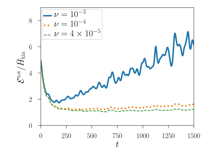
Figure 6: Evolution of the ratio of enstrophy with unsigned kinetic helicity for different viscosities $\nu$ against simulation time.

V.2 Kinetic Helicity and Kinetic Energy

Next we study the relation between the integrated kinetic helicity and kinetic energy. In order to be consistent with the helicity calculation we need to calculate the energy also in the rest frame, with velocity $\mbox{\boldmath$u$}{}+\mbox{\boldmath$U$}{}$ and vorticity $\mbox{\boldmath$\omega$}{}+\bm{\Omega}$. With a much larger $U$ compared to $u$ (since $|\mbox{\boldmath$U$}{}|\propto r\in[45,65]$), the energy would be dominated by the background velocity. So in order to prevent that any change is obscured by the large background contribution, we compute the “free” kinetic energy instead, that is we subtract the energy of the background field

$$E_{\rm kin}^{\rm free}=\int_{V}\rho\left(\frac{1}{2}\mbox{\boldmath$u$}{}^{2}+\mbox{\boldmath$u$}{}\cdot\mbox{\boldmath$U$}{}\right)r\ {\rm d}{}r\ {\rm d}{}\theta\ {\rm d}{}z.$$ (14)

Due to the Coriolis force,inertial waves are induced whose dominant frequency is determined by the background rotation rate. Combined with a background velocity $U$ that is large compared to $u$ we see large periodic fluctuations of $E_{\rm kin}^{\rm free}$. Therefore, to reveal the limiting behaviour we compute running means for our values $E_{\rm kin}^{\rm free}/\bar{H}_{\rm kin}$ over $100$ time units.

Although a strict lower limit for the kinetic energy is not known, we observe that the ratio of the free kinetic energy and unsigned kinetic helicity tends asymptotically to a non-zero value (Figure 7) with the limit value of ca. 0.0025. This is so striking that it leads us to conclude that there exists a lower limit for the kinetic energy in the presence of unsigned kinetic helicity.

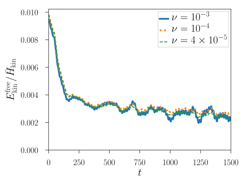
Figure 7: Evolution of the ratio of free kinetic energy with unsigned kinetic helicity for different viscosities $\nu$ against simulation time. Here we use a running mean with window of $100$ time units to smooth out oscillatory behavior induced by inertial waves.

This finding is complementary to previous findings on helical turbulent flows in rotating frames (Teitelbaum and Mininni, 2011, 2009) where the authors studied the effect of net kinetic helicity and rotation on the kinetic energy decay. They find that, while helicity in a non-rotating frame does not affect the energy decay, in a rotating frame, helicity poses restrictions leading to a slower decay.

VI Field Topology

Our simulated configuration consists of two vortex rings. However, we aim to compare our results to previous works using three pairs of such vortex rings (e.g. Wilmot-Smith, Hornig, and Pontin (2009)). Therefore, for the discussion in this section, we will make use of the periodicity in the $z$-direction and construct such a braid by following vortex streamlines over three periods.

VI.1 Simplification of the Topology

In order to analyze the changing topology of the vorticity field we integrate – at each instant of time – a set of vorticity field lines starting from a fixed grid of starting points on the lower boundary ($z=-16$). Naively we would expect the vortex field to simplify into a homogeneous field in the $z$-direction (due to the net-zero helicity this should be the lowest-energy state). However, as time progresses, and the field lines reconnect due to the finite viscosity, the topology of the field simplifies (Figure 8) not to an untwisted field, but – similar to the magnetic case (Pontin et al., 2011; Yeates, Hornig, and Wilmot-Smith, 2010) – into two large-scale vorticity tubes containing twisted vortex lines, of opposite twist (swirl). The fact that this final state mirrors closely the final state of the relaxation of a magnetic braid in a plasma (with the same initial topology) suggests that some unifying underlying conservation principle is shared between the two systems.

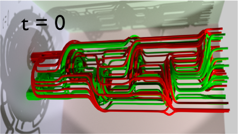
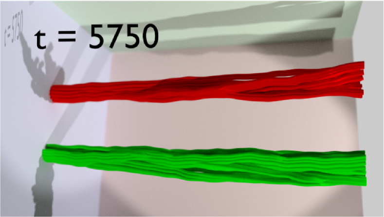
Figure 8: Vortex streamlines in the rest frame (with background vorticity) for the $\nu=4\times 10^{-5}$ case at time $t=0$ (upper panel) and $t=5750$ (lower panel). In order to compare with previous simulations of magnetic braids we repeat our computational domain in the $z$-direction (horizontal in these plots) three times. The initial braid is largely unbraided and the final configuration consists of two separated vortex tubes of opposite twist.

VI.2 Field Line Helicity

The above-mentioned simplification of the topology is effectively quantified/visualized by plotting the kinetic field line helicity, constructed as follows. Due to the positive $z$-component of the vorticity, any field line starting at the lower domain boundary will end at the top boundary. This way we can find a one–to–one mapping between the boundaries. For that we trace $256^{2}$ field lines starting at the lower boundary that are equally spaced in the radial direction $r\in[49,60]$ and the azimuthal direction $\theta\in[-0.1,0.1]$. We use those field lines to compute the kinetic field line helicity

$$\mathcal{A}(x_{0},y_{0})=\int_{C}\frac{((\mbox{\boldmath$u$}{}+\mbox{\boldmath$U$}{})(x,y,z)\cdot(\mbox{\boldmath$\omega$}{}(x,y,z)+\bm{\Omega})}{(\mbox{\boldmath$\omega$}{}(x,y,z)+\bm{\Omega})_{z}}\ {\rm d}{}z,$$ (15)

where $x(x_{0},y_{0},z)$ and $y(x_{0},y_{0},z)$ are the mapped points along the vorticity field line paths, $C$ (Yeates and Hornig, 2011a). This measures the amount of winding (Berger, 1988) of each field line around all other field lines and gives us a picture about the distribution of the helicity even in cases where its net value vanishes.

Since our vortex braid is highly tangled, the distribution of the field line helicity at initial time shows some complexity at relatively small scales (Figure 9, upper panel). As time progresses and the field lines reconnect, the distribution simplifies greatly into two separate regions with opposite field line helicity (Figure 9, lower panel), that correspond to the two flux tubes of opposite twist/swirl described above.

Indeed, Yeates and Hornig (2011a) showed that there is a connection between the reconnection rate and the source term of the field line helicity, which for the hydrodynamic case takes the form

$$\frac{{\rm D}{}\mathcal{A}}{{\rm D}{}t}=-\nu\int_{C}\frac{\mbox{\boldmath$\nabla$}{}\times\mbox{\boldmath$\omega$}{}\cdot(\mbox{\boldmath$\omega$}{}+\bm{\Omega})}{|(\mbox{\boldmath$\omega$}{}+\bm{\Omega})|}\ {\rm d}{}l,$$ (16)

where $l$ is the arc length along the vorticity line $C$.

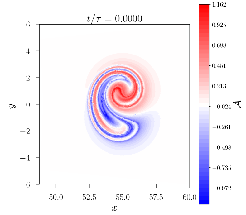
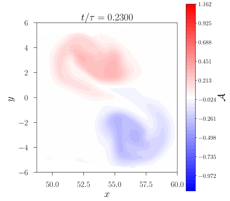
Figure 9: Field line helicity distribution in the rest frame (with background vorticity) of the vortex field at initial time (upper panel) and normalized time $t/\tau=0.230$ (lower panel), which corresponds to $t=5750$ (see equation (8)), for the run with $\nu=4\times 10^{-5}$. In order to compare with previous simulations of magnetic braids we repeat our computational domain in the $z$-direction three times. Here we use $x=r\cos{(\theta)}$ and $y=r\sin{(\theta)}$ for the coordinates.

VII Conclusions

We performed simulations of the relaxation of non-helical vortex braids in a cylindrical wedge domain for a viscous fluid. While the kinetic energy viscously decays, we observe an increase in the integrated norm of the kinetic helicity density at dynamical times. This increase is due to the reconnection of the vortex field lines at early times and conincides with the time the flux rings that generate the braid collide.

The most striking finding of our study is that the unsigned kinetic helicity appears to constrain the relaxation of the studied vortex braid. Specifically, the ratio of the kinetic energy to unsigned helicity approaches a non-zero value at late times that is independent of the viscosity. This implies the presence of additional topological constraints on the hydrodynamic relaxation process, that may be related to those discovered recently for the magnetohydrodynamic system. In magnetohydrodynamics it is known that the presence of magnetic helicity imposes a lower bound for the magnetic energy. At the same time, we know from numerical experiments that topologically non-trivial magnetic braids are not free to decay, even in the case of net-zero magnetic helicity. The presence of additional topological constraints, such as preservation of the fixed point index or the field line helicity, restrict the field’s decay (Yeates, Hornig, and Wilmot-Smith, 2010; Yeates and Hornig, 2011b; Yeates, Russell, and Hornig, 2015). For the hydrodynamic case, such relations between the kinetic energy and kinetic helicity are not known, but the present results strongly suggest their existence.

However, for the enstrophy we derived a lower bound in presence of unsigned kinetc helicity. This relation is similar to the magnetohydrodynamic case, but with the enstrophy replacing the energy. Our simulations clearly confirm the validity of this analytical result and we suggest that this relation should be taken into account when studying the relaxation of hydrodynamical systems.

In addition to the above, we discovered another close parallel between the final states of our vortex braid relaxation and magnetic braid relaxations. Specifically, for the same braid topology, the two cases relax towards a topologically equivalent final state, as revealed by plotting, e.g., the field line helicity (Figure 9). The fact that the final states of these two very different relaxation processes are analogous for the braid considered suggests that the constraints are likely also related to one another, and the exploration of these topological constraints in the hydrodynamic system will be an important area of future study.

Data Availability

Raw data were generated using HPC facilities. Derived data supporting the findings of this study are available from the corresponding author upon reasonable request.

Appendix A Construction of Vortex Tubes

In our simulations, the variables that are solved for are not the vorticity $\omega$, but the velocity $u$. So, we need to specify our initial conditions in terms of $u$ with $\mbox{\boldmath$\nabla$}{}\times\mbox{\boldmath$u$}{}=\mbox{\boldmath$\omega$}{}$. Yet, for a given vorticity $\omega$ we can find different velocities $u$ such that $\mbox{\boldmath$\nabla$}{}\times\mbox{\boldmath$u$}{}=\mbox{\boldmath$\omega$}{}$, similar to the gauge freedom for the magnetic vector potential $A$ with the magnetic field $\bm{B}=\mbox{\boldmath$\nabla$}{}\times\mbox{\boldmath$A$}{}$. However, it is not desirable to use the expression for the vector potential from Wilmot-Smith, Hornig, and Pontin (2009) for our velocity field $u$ as it is not divergence-free, leading to unwanted compression.

In order to construct a divergence-free flow field we use the solutions of the Biot-Savart integral for a singular vortex ring (see Jackson (2007), section 5.5). We then construct the vortex ring from a sum (integral) of infinitely many infinitesimally thin vortex rings. For that we compute a potential $C$ such that $\mbox{\boldmath$u$}{}=\alpha\mbox{\boldmath$\nabla$}{}\times(C\mbox{\boldmath$e$}{}_{\theta})$ which results in a divergence-free velocity field by construction.

We first construct the potential $C_{0}$ for a single vortex ring in a coordinate system with origin at the ring’s center. In a later step we will shift (transform) this potential to its actual position. Our coordinates here are $(r_{0},\theta_{0},z_{0})$. Here, the potential $C_{0}(r_{0},\theta_{0},z_{0})$ is the double integral

$$C_{0}(r_{0},\theta_{0},z_{0})=\int_{-8}^{8}{\rm d}{}z_{0}^{\prime}\int_{0}^{5}{\rm d}{}r_{0}^{\prime}\sqrt{2}r_{0}^{\prime}e^{-r_{0}^{\prime 2}/2-z_{0}^{\prime 2}/4}\Psi,$$ (17)

with

$$\Psi=\frac{r_{0}^{\prime}\left((\kappa^{2}+2)K(\kappa)-2E(\kappa)\right)}{\pi\sqrt{r_{0}^{\prime 2}+r_{0}^{2}+(z_{0}-z_{0}^{\prime})^{2}+2r_{0}^{\prime}r_{0})}\kappa^{2}},$$ (18)

with the complete elliptical integral of the first kind $K(\kappa)$, complete elliptical integral $E(\kappa)$ and

$$\kappa=2\sqrt{\frac{r_{0}^{\prime}r_{0}}{r_{0}^{\prime 2}+r_{0}^{2}+(z_{0}-z_{0}^{\prime})^{2}+2r_{0}^{\prime}r_{0}}}.$$ (19)

We choose to integrate in $z_{0}^{\prime}$ from $-8$ to $8$ and in $r^{\prime}_{0}$ from $0$ to $5$, as beyond those integration intervals the integrand is sufficiently small to be neglected from the integration. For more details about this construction see Jackson (2007), section 5.5.

This gives us the vector potential $C_{0}(r_{0},\theta_{0},z_{0}){\bf e}_{\theta_{0}}$ in the centered coordinate system $(r_{0},\theta_{0},z_{0})$. In order to construct the braid we make a coordinate transformation so that our ring is centered at $r=R_{0},\theta=\Theta$. The coordinates transform according to

$$r_{0} = \sqrt{r^{2}+R_{0}^{2}-2rR_{0}\cos(\theta-\Theta)}$$ (20)

$$\theta_{0} = \arctan(\sin(\theta-\Theta)/\cos(\theta-\Theta)-R_{0}/r)$$ (21)

$$z_{0} = z,$$ (22)

while the vector potential transforms as

$$C_{r}(r,\theta,z) = \frac{-C_{0}(r_{0},\theta_{0},z_{0})R_{0}\sin(\theta-\Theta)}{\sqrt{-2R_{0}r\cos(\theta-\Theta)+R_{0}^{2}+r^{2}}}$$ (23)

$$C_{\theta}(r,\theta,z) = \frac{C_{0}(r_{0},\theta_{0},z_{0})(r-R_{0}\cos(\theta-\Theta))}{\sqrt{-2R_{0}r\cos(\theta-\Theta)+R_{0}^{2}+r^{2}}}.$$ (24)

After this transformation we apply the curl operator in the wedge domain and obtain the initial velocity in the wedge domain. The resulting vortex rings have a minor and major radius of ca. $1$.

Appendix B Inequality for the Unsigned Helicity

The relation between unsigned kinetic helicity and enstrophy is derived using the Poincaré inequality

$$\left(\int_{V}\|\mbox{\boldmath$u$}{}\|^{2}\ {\rm d}{}^{3}x\right)^{1/2}\leq\frac{1}{\lambda}\left(\int_{V}\|\mbox{\boldmath$\omega$}{}\|^{2}\ {\rm d}{}^{3}x\right)^{1/2},$$ (25)

which holds for every differentiable field, such that $\mbox{\boldmath$\omega$}{}=\mbox{\boldmath$\nabla$}{}\times\mbox{\boldmath$u$}{}$. Here $\lambda$ is the smallest positive eigenvalue of the curl operator.

We can now apply the Cauchy-Schwarz inequality to the unsigned kinetic helicity density to obtain

$$\int_{V}\left|{\mbox{\boldmath$\omega$}{}\cdot\mbox{\boldmath$u$}{}}\right|\,{\rm d}{}^{3}x\leq\int_{V}\|\mbox{\boldmath$\omega$}{}\|\|\mbox{\boldmath$u$}{}\|\ {\rm d}{}^{3}x,$$ (26)

and apply it a second time to the integral ($L^{2}$-norm version)

$$\int_{V}\left|{\mbox{\boldmath$\omega$}{}\cdot\mbox{\boldmath$u$}{}}\right|\,{\rm d}{}^{3}x\leq\left(\int_{V}\|\mbox{\boldmath$\omega$}{}\|^{2}\ {\rm d}{}^{3}x\right)^{1/2}\left(\int_{V}\|\mbox{\boldmath$u$}{}\|^{2}\ {\rm d}{}^{3}x\right)^{1/2}.$$ (27)

Eventually we use the Poincaré inequality to obtain

$$\int_{V}\left|{\mbox{\boldmath$\omega$}{}\cdot\mbox{\boldmath$u$}{}}\right|\,{\rm d}{}^{3}x\leq\frac{1}{\lambda}\int_{V}\|\mbox{\boldmath$\omega$}{}\|^{2}\ {\rm d}{}^{3}x.$$ (28)

This leaves us with the inequality

$$\bar{H}_{\rm kin}\leq\frac{1}{\lambda}\mathcal{E}.$$ (29)

References

- Moffatt (1969) H. K. Moffatt, “The degree of knottedness of tangled vortex lines,” J. Fluid Mech. 35, 117–129 (1969).
- Moffatt (1992) H. K. Moffatt, “Relaxation under topological constraints,” in Topological Aspects of the Dynamics of Fluids and Plasmas, edited by H. K. Moffatt, G. M. Zaslavsky, P. Comte, and M. Tabor (Springer Netherlands, Dordrecht, 1992) pp. 3–28.
- Scheeler et al. (2014) M. W. Scheeler, D. Kleckner, D. Proment, G. L. Kindlmann, and W. T. M. Irvine, “Helicity conservation by flow across scales in reconnecting vortex links and knots,” P. Natl. Acad. Sci. USA 111, 15350–15355 (2014).
- Scheeler et al. (2017) M. W. Scheeler, W. M. van Rees, H. Kedia, D. Kleckner, and W. T. M. Irvine, “Complete measurement of helicity and its dynamics in vortex tubes,” Science 357, 487–491 (2017).
- Kerr (2018) R. M. Kerr, “Topology of interacting coiled vortex rings,” Journal of Fluid Mechanics 854, R2 (2018).
- Ashurst and Meiron (1987) W. T. Ashurst and D. I. Meiron, “Numerical study of vortex reconnection,” Phys. Rev. Lett. 58, 1632–1635 (1987).
- Melander and Hussain (1989) M. V. Melander and F. Hussain, “Cross-linking of two antiparallel vortex tubes,” Phys. Fluids 1, 633–636 (1989).
- Kida, Takaoka, and Hussain (1991) S. Kida, M. Takaoka, and F. Hussain, “Collision of two vortex rings,” J. Fluid Mech. 230, 583–646 (1991).
- van Rees, Hussain, and Koumoutsakos (2012) W. M. van Rees, F. Hussain, and P. Koumoutsakos, “Vortex tube reconnection at Re = 104,” Phys. Fluids 24, 075105–075105 (2012).
- McGavin and Pontin (2018) P. McGavin and D. I. Pontin, “Vortex line topology during vortex tube reconnection,” Phys. Rev. Fluids 3, 054701 (2018).
- Zhao et al. (2021) X. Zhao, Z. Yu, J.-B. Chapelier, and C. Scalo, “Direct numerical and large-eddy simulation of trefoil knotted vortices,” J. Fluid Mech. 910, A31 (2021).
- Hornig (2001) G. Hornig, “The Geometry of Reconnection,” An Introduction to the Geometry and Topology of Fluid Flows, Ed.: R.L. Ricca, Kluwer (2001).
- McGavin and Pontin (2019) P. McGavin and D. I. Pontin, “Reconnection of vortex tubes with axial flow,” Phys. Rev. Fluids 4, 024701 (2019).
- Yeates and Hornig (2013) A. R. Yeates and G. Hornig, “Unique topological characterization of braided magnetic fields,” Phys. Plasmas 20, 012102 (2013).
- Yeates and Hornig (2011a) A. R. Yeates and G. Hornig, “A generalized flux function for three-dimensional magnetic reconnection,” Phys. Plasmas 18 (2011a), http://dx.doi.org/10.1063/1.3657424.
- Candelaresi, Pontin, and Hornig (2017) S. Candelaresi, D. I. Pontin, and G. Hornig, “Quantifying the tangling of trajectories using the topological entropy,” Chaos 27, 093102 (2017).
- Yeates, Hornig, and Wilmot-Smith (2010) A. R. Yeates, G. Hornig, and A. L. Wilmot-Smith, “Topological constraints on magnetic relaxation,” Phys. Rev. Lett. 105, 085002 (2010).
- Wilmot-Smith, Hornig, and Pontin (2009) A. L. Wilmot-Smith, G. Hornig, and D. I. Pontin, “Magnetic braiding and parallel electric fields,” Astrophys. J. 696, 1339 (2009).
- Note (1) Github.com/pencil-code/.
- Brandenburg and Dobler (2002) A. Brandenburg and W. Dobler, “Hydromagnetic turbulence in computer simulations,” Comput. Phys. Commun. 147, 471–475 (2002).
- Kerr (2013) R. M. Kerr, “Fully developed hydrodynamic turbulence from a chain reaction of reconnection events,” Procedia IUTAM 9, 57–68 (2013).
- McKeown et al. (2018) R. McKeown, R. Ostilla-Mónico, A. Pumir, M. P. Brenner, and S. M. Rubinstein, “Cascade leading to the emergence of small structures in vortex ring collisions,” Phys. Rev. Fluids 3, 124702 (2018).
- Yao and Hussain (2020) J. Yao and F. Hussain, “A physical model of turbulence cascade via vortex reconnection sequence and avalanche,” J. Fluid Mech. 883, A51 (2020).
- Nguyen and Duong (2021) V. L. Nguyen and V. D. Duong, “Vortex ring-tube reconnection in a viscous fluid,” Phys. Fluids 33, 015122 (2021).
- Pontin et al. (2011) D. I. Pontin, A. L. Wilmot-Smith, G. Hornig, and K. Galsgaard, “Dynamics of braided coronal loops. II. Cascade to multiple small-scale reconnection events,” Astron. Astrophys. 525, A57 (2011).
- Yeates, Russell, and Hornig (2015) A. R. Yeates, A. J. B. Russell, and G. Hornig, “Physical role of topological constraints in localized magnetic relaxation,” P. Roy. Soc. A-Math. Phy. 471, 20150012–20150012 (2015).
- Arnold (1986) V. I. Arnold, “The asymptotic Hopf invariant and its applications,” Sel. Math. Sov. 5, 327–345 (1986).
- Brandenburg, Dobler, and Subramanian (2002) A. Brandenburg, W. Dobler, and K. Subramanian, “Magnetic helicity in stellar dynamos: new numerical experiments,” Astron. Nachr. 323, 99–122 (2002).
- Del Sordo, Candelaresi, and Brandenburg (2010) F. Del Sordo, S. Candelaresi, and A. Brandenburg, “Magnetic-field decay of three interlocked flux rings with zero linking number,” Phys. Rev. E 81, 036401 (2010).
- Candelaresi and Brandenburg (2011) S. Candelaresi and A. Brandenburg, “Decay of helical and nonhelical magnetic knots,” Phys. Rev. E 84, 016406 (2011), arXiv:1103.3518 [astro-ph.SR] .
- Arnold and Khesin (2013) V. Arnold and B. Khesin, Topological Methods in Hydrodynamics (Springer New York, 2013).
- Teitelbaum and Mininni (2011) T. Teitelbaum and P. D. Mininni, “The decay of turbulence in rotating flows,” Phys. Fluids 23, 065105 (2011).
- Teitelbaum and Mininni (2009) T. Teitelbaum and P. D. Mininni, “Effect of helicity and rotation on the free decay of turbulent flows,” Phys. Rev. Lett. 103, 014501 (2009).
- Berger (1988) M. A. Berger, “An energy formula for nonlinear force-free magnetic fields,” Astron. Astrophys. 201, 355–361 (1988).
- Yeates and Hornig (2011b) A. R. Yeates and G. Hornig, “Dynamical constraints from field line topology in magnetic flux tubes,” J. Phys. A-Math. Theor. 44, 265501 (2011b).
- Hunter (2007) J. D. Hunter, “Matplotlib: A 2d graphics environment,” Comput. Sci. Eng. 9, 90–95 (2007).
- Note (2) Github.com/SimonCan/BlenDaViz.
- Jackson (2007) J. Jackson, “Classical electrodynamics, 3rd ed,” (Wiley India Pvt. Limited, 2007) Chap. 5.5.