Climate Modeling and Bifurcation

Abstract

Many papers and monographs were written about the modeling the Earth climate and its variability. However there is still an obvious need for a module that presents the fundamentals of climate modeling to students at the undergraduate level. The present educational paper attempts to fill in this gap. To this end we collect in this paper the relevant climate data and present a simple zero and one dimensional models for the mean temperature of the Earth. These models can exhibit bifurcations from the present Earth climate to an ice age or a ”Venus type of climate”. The models are accompanied by Matlab programs which enable the user to change the models parameters and explore the impact that these changes might have on their predictions on Earth climate.

1 Introduction

The Earth climate and its variations has always been of great interest to Humans as it has major impact on Human activities. In this paper we present prototype models for the mean temperature of the Earth which will enable us to explore possible bifurcations in the Earth climate which might due in part to anthropogenic emissions and natural forcing processes. These model are based in part on the approach presented in [1, 4]. More elaborate and sophisticated models are available in the literature [3, 5, 4].

Much was written lately about the gradual change in the mean temp of the earth due to Human intervention which is expected to range by 1-2 degrees by the end of this century. However the real danger of these changes is that they may lead to a rapid major change in the Earth climate (viz. climate bifurcation [6]) in the same way that a rubber band snaps suddenly when it is over stretched or a sudden snow avalanche occurs on the slopes of a mountain.

The Earth climate system is composed of the following components: land, biosphere, atmosphere, ocean and the cryosphere (ice and frozen water), These components display a broad range of variability on temporal and spatial scales such as the Dansgaard-Oeschger cycles which occur quasi-periodically on a millennial time scale or the El Niño-Southern Oscillation in the equatorial Pacific. Thus a refined model of such a complex system requires vast amounts of data and elaborate sophistication. In the following we stick to the basics.

The plan of the is as follows: In Sec 2 we introduce the basic concepts needed for climate modeling. Sec $3$ presents the relevant climate data. The zero dimensional model and it predictions are discussed in Sec $4$. The one dimensional climate model is presented in Sec $5$. Sec $6$ discusses some attempts to mitigate the effects of the greenhouse effect. We end up in Sec $7$ with some conclusions.

2 Some Basics

In this section we introduce some basic concepts and data needed for the modeling of the Earth climate.

2.1 The Albedo

When radiation impinges on a (perfect) mirror all of this radiation is reflected back and the temperature of the mirror remains unchanged. On the other hand is such radiation impinges on a (perfect) black body all of the radiation is absorbed by that body. In general however some of this radiation is absorbed by the body and some is reflected back. We say that in this case we are dealing with a ”grey body”. In general the albedo of a body is the percentage of radiation that is reflected back by the body into space. Thus for a perfect mirror the albedo is $1$ and for a black body the albedo is zero. For a grey body the albedo is a number between zero and one.

The Earth is a grey body. However it albedo changes with time due to snow and ice cover, vegetation and Human activities (e.g. the paving of asphalt roads)

2.2 Greenhouse Gases and Clouds

Radiation from the Sun reaches Earth (mostly) in the visible part of the spectrum (viz. wave lengths in the range of $380\times 10^{-9}$ - $750\times 10^{-9}$ meters). Radiation with shorter wavelengths is absorbed (mostly) by the Van-Allen belts. The Earth absorbs part of this radiation and emit it back in the infra red part of the spectrum (with wave lengths n the range of $7.5\cdot 10^{-7}-1\cdot 10^{-4}$ meters. If the Earth had no atmosphere this radiation will be reflected into space. However in the Earth atmosphere some trace gases such as Carbon dioxide ($CO_{2}$), Methane ($CH_{4}$) and water vapor can absorb this radiation and reflect it back to Earth [4]. This leads to a warming of the Earth surface. (Fig. $1$ presents the absorption spectra of several trace gases- source of this figure is unknown).

NOAA Earth System Research Laboratory (Global Monitoring Division) has been monitoring the concentration of the trace gases in the atmosphere from an observation station on Mona Loa mountain in Hawaii and globally[7, 8, 9] by averaging these concentrations as measured by observation stations throughout the globe. This data is shown in Figs. $2,3,4$ (courtesy of ”NOAA Global Monitoring Division’) they demonstrate the almost linear increase in the concentrations of $CO_{2}$ and $CH_{4}$ over many years which can be attributed Human activities.

The effect of clouds in this scenario is dual. First they block the Sun radiation and reflect it into space. At the same time they also reflect the Earth infra red radiation back to Earth. There is still on going debate in the scientific community as to which of these two process is more prominent for the determination of the Earth energy balance.

2.3 Stefan-Boltzmann Law

Stefan–Boltzmann states that the power radiated from a black body as a function of its temperature is given by

$$P=\sigma AT^{4}$$

where $A$ is the body surface area, T is it temperature and $\sigma=5.67\times 10^{-8}$ $Watts/(m^{2}K^{4})$ is the Stefan–Boltzmann constant.

For a grey body $P$ has to multiplied by the “grayness” coefficient of the body.

3 A Model for the Mean Temperature of the Earth

We enumerate here the data that is needed to model the mean temperature of the Earth and then assemble these into model equations.

1. The Sun Forcing

   The rate at which energy from the Sun reaches the top of Earth’s atmosphere is called “total solar irradiance” (or TSI)[10, 16, 17]. TSI fluctuates slightly from day to day and week to week. In addition to these rapid, short-term fluctuations, there is an 11-year cycle in TSI measurements related to “sunspots” (a part of the Sun’s surface that is temporarily cooler and darker than its neighboring regions).

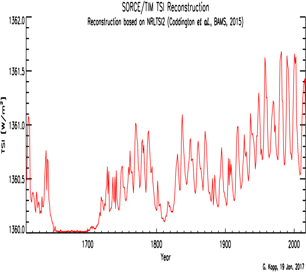
Figure 5: Solar Irradiance

   The evidence shows that although fluctuations in the amount of solar energy reaching our atmosphere do influence our climate, the global warming trend of the past six decades cannot be attributed to changes in the Sun output. Fig. 5 which was compiled by Professor G. Kopp[17] (and reproduced here with his permission) is a graph of TSI for the last 400 years. It shows clearly the ”small ice age” during the 17th century. This TSI average is referred to as the ’solar constant’, in power (watts) per square meter.

   From a practical point of view we can consider the Sun rays arriving in parallel to Earth. This energy flux was measured to be $F_{s}\approx 1362$ $Watt/m^{2}$ [10, 16, 17]. However the cross section of the Earth to this flux is $\pi R^{2}$ while it surface area is $4\pi R^{2}$. Therefore we divide this flux be $4$ when we compute the average temperature of the Earth.

   The average albedo of the Earth from the upper atmosphere, its planetary albedo, is $30$–$35\%$ because of cloud cover, but widely varies locally across the surface because of different geological and environmental features.

2. the Albedo

   The albedo of the earth is constantly changing. We shall model it as having two values:

   $$\alpha_{M}=0.85,\,\,\,\,\alpha_{m}=0.25;$$

   where $\alpha_{M}$ is the albedo for Earth covered by snow,ice (frozen Earth), and $\alpha_{m}=0.25$ is the albedo for the part of the Earth that is not covered by snow, ice etc (i.e not frozen). The Earth will be considered as frozen if it mean temperature is below $T_{1}=240$ Kelvin and unfrozen if it mean temperature is over $T_{2}=275$ Kelvin. In between $T_{1}$ and $T_{2}$ we use linear interpolation to compute the albedo

   $$\alpha(T)=\frac{\alpha_{m}-\alpha_{M}}{T_{2}-T_{1}}(T-T_{1})+\alpha_{M}$$ (3.1)

   (Observe that the effect of changes in the vegetation of the Earth is not taken (directly) into consideration in this model)

   More elaborate models for the earth albedo are available[2, 4] and satellites are being used currently to give accurate real time data on its value. It is estimated that the average albedo of the Earth (viz. planetary albedo) is $30\%$ to $35\%$ because of cloud cover and the effect of trace gases, but it varies widely across the surface because of different geological and environmental features.

3. Clouds and the Greenhouse factor

   Let $T_{0}$ be the ambient temperature for green house effect, and $\kappa(T)$ the cloud cover due to the green house effect. (Without the greenhouse effect the mean temperature of the Earth will be $\approx 240$ Kelvin and effectively there will no cloud cover)

   The incoming radiation from the Sun that is absorbed by Earth is

   $$R_{in}=\frac{F_{s}A}{4}(1-\alpha(T))$$

   where $A$ is the surface area of the Earth. The outgoing infra red radiation from Earth is

   $$R_{out}=\sigma Ag(T)T^{4}$$

   where $g(t)$ is a lump sum parameter that represents the impact of the greenhouse gases and clouds. This parameter was modeled (empirically) by Sellers[1] as

   $$g(T)=1-\kappa\tanh[(T/T_{0})^{6}],\,\,\,\,\kappa=0.5$$

   where $T_{0}\approx 275$ Kelvin. This expression implies that as $T$ increases $g(T)$ decreases and the greenhouse effect becomes stronger ($R_{out}$ decreases)

4 Zero-dimensional Climate Model

If we denote by $C$ the heat capacity of the Earth then by the law of energy conservation it follows that

$$C\frac{dT}{dt}=R_{in}-R_{out}$$ (4.2)

at equilibrium (viz. Steady state) $\frac{dT}{dt}=0$ and we must have therefore that $R_{in}-R_{out}=0$.

4.1 Model Predictions

If the Earth atmosphere was totally transparent with no greenhouse gases (or if the Earth had no atmosphere) then $g(T)=1$. The percentage of Sun energy that is reflected by the Earth into space (viz. albedo) is estimated to be $\alpha(T_{E})=0.3$. The equilibrium mean temperature of the Earth $T_{E}$ will have to satisfy then

$$\frac{F_{s}A}{4}(1-\alpha(T_{E}))-\sigma Ag(T_{E})T_{E}^{4}=0$$ (4.3)

The solution of this equation yields $T_{E}=255$ Kelvin which is well below the freezing point of water. Thus the Earth will be covered by snow and ice. It follows then that the difference between this value of $T_{E}$ and the (estimated) current mean temperature of $T_{0}=284.9$ Kelvin is due to the greenhouse effect. To find the value of $g(T)$ that leads to this equilibrium temperature we substitute $T_{0}=284.9$ in (4.3) and solve for $g$ (with $\alpha(T_{E})=0.3$). We find that the current value of $g$ is $0.65$.

To investigate further the insights that can obtained from this model we wrote a Matlab program $mean03.m$ that implements it. At first we used this program, with the model parameters that are quoted above[1, 4]. Using this program with an initial (mean) temperature of $285$ Kelvin we obtained Fig. $6$ ($20$ years simulation). This initial mean temperature is based on data which was collected by NASA which shows that the Earth mean surface temperature in $2017$ was $14.9C$. Fig. $6$ shows a steady increase in the average temperature of the Earth for the first few years which then stabilizes around $305$ Kelvin. (This program is available for download from the author web page [14]).

Many of the original parameters[1, 4] used in this program are estimates (at best) and are changing with time. Therefore one can use this program to probe also for the dependence (or sensitivity) of the results to the values of the various parameters of this model. As an example we varied the value of $T_{2}$ in (3.1) from $275$ (original value) to $296.11$ with no substantial changes in the results. However if we increase $T_{2}$ to over $296.12$ we obtain Fig $7$ where the Earth mean temperature plunges to an ice age. Thus the model exhibits a climate bifurcation if $T_{2}$ is in between $[296.11,296.12]$.

5 One-dimensional Climate Model

In this model the Earth temperature is considered to be a function of time and latitude $\theta$. Using this one dimensional model it is possible to study the oscillation of the Earth climate between ice ages in the past.

To present this model we need to develop first, two mathematical formulas.

5.1 Area of a Strip on a Circle

We want to find a formula for the area of a strip on a circle of radius $R$ that is enclosed between the equator and south of latitude line $\theta$ (see Fig $8$). This area equals the sum of the area of the rectangle $2R\cos\theta\sin\theta$ and the area enclosed by equator and the two arcs of the circle. Hence the total area of the strip is

$$A(\theta)=2R^{2}\cos\theta\sin\theta+2\displaystyle\int_{Rcos\theta}^{R}\sqrt{R^{2}-x^{2}}dx=R^{2}(\cos\theta\sin\theta+\theta)=R^{2}\left(\frac{\sin(2\theta)}{2}+\theta\right).$$ (5.4)

It follows that the area of a strip on the circle between $\theta$ and $\theta+d\theta$ is

$$dA=\frac{dA(\theta)}{d\theta}d\theta=R^{2}(\cos(2\theta)+1)d\theta.$$ (5.5)

5.2 Area of a ”polar cap” on a Sphere

The formula for the area north of a line of latitude $\theta$ can be computed directly as in the previous subsection. It is given by,

$$S(\theta)=2\pi R^{2}(1-\sin(\theta))$$ (5.6)

The area enclosed by a strip on the sphere between $\theta$ and $\theta+d\theta$ is

$$\Delta S=2\pi R^{2}(1-\sin(\theta))-2\pi R^{2}(1-\sin(\theta+\Delta\theta)$$ (5.7)

$$=2\pi R^{2}(\sin(\theta+\Delta\theta)-\sin(\theta))=2\pi R^{2}\frac{\sin(\theta+\Delta\theta)-\sin(\theta)}{\Delta\theta}\Delta\theta$$

which in the limit $\Delta\theta\rightarrow 0$ yields

$$dS=2\pi R^{2}\cos(\theta)d\theta$$ (5.8)

5.3 Steady State 1-dimensional Model

To derive a one dimensional steady state model for the Earth temperature as a function of $\theta$ we consider a strip on the Earth between $\theta$ and $\theta+d\theta$. The cross section of this strip to the sun radiation is given by (5.5) . The incoming radiation from the Sun that is absorbed by this strip on Earth is

$$R_{in}={F_{s}}(1-\alpha(T(\theta))dA={F_{s}}(1-\alpha(T(\theta))R^{2}(\cos(2\theta)+1)d\theta$$ (5.9)

The outgoing infra red radiation from Earth from this strip is

$$R_{out}=\sigma g(T(\theta)T(\theta)^{4}dS=\sigma g(T(\theta))T(\theta)^{4}(2\pi R^{2}\cos(\theta)d\theta)$$ (5.10)

Hence when the system is out of equilibrium and $T=T(t,\theta)$ we have by the law of energy conservation

$$C\frac{\partial T}{\partial t}=k\nabla T+R_{in}(\theta)-R_{out}(\theta)$$ (5.11)

where $R_{in}$ and $R_{out}$ are given by (5.9) and (5.10) respectively. The term $k\nabla T$ represents the heat transport (or diffusion) due to temperature difference (viz. gradient) in the different latitudes (due to atmospheric and ocean currents). The coefficient $k$ is called the diffusion coefficient. Without this meridional heat transport the equator will become increasingly warmer while the poles increasingly colder. An approximation of this term (that is used by some authors) is to replace it by a term proportional to the temperature difference ${\bar{k}}(T(t,\theta)-T_{ave})$ where $T_{ave}$ is an estimate for the global temperature average.

We observe also that this model equation does not take into account the change in the Earth tilt with respect to the Sun at different seasons.

Neglecting the diffusion term in (5.11) we must then have at the steady state $R_{in}=R_{out}$ and the following expression for $T(\theta)$

$${F_{s}}(1-\alpha(T(\theta))\cos(\theta)=\pi\sigma g(T(\theta))T(\theta)^{4}$$ (5.12)

This equation have to be solved either graphically or iteratively since the values of $\alpha(T)$ and $g(T)$ depend on the final equilibrium temperature.

The results of this model are rather unusual. If one starts the simulation from above the freezing temperature (e.g. 280 Kelvin) one obtains Fig $8$ where at least part of Earth is well above the freezing point. On the other hand if one starts the simulation from $240$ Kelvin one finds that the Earth is a frozen ball (see Fig $9$). This demonstrates that this model exhibits the existence of two stable climates, one is ”warm” and the other is ”frozen”. The first corresponds to the present climate while the second corresponds to an ice age. Matlab programs mod03.m and mod04.m which implement these results can be downloaded from [15]

If the parameters of the system change (e.g if $F_{S}$ changes) ”slightly” and the Earth is at the warm stable climate it will stay at warm temperatures. On the other hand if it is in the cold stable climate it will remain at an ice age. The transition from one stable climate to another occurs due to variations in the solar output and the $CO_{2}$ (and other greenhouse gases) concentration cycle in the atmosphere.

In this model the average Earth temperature as a function of the system variables follow a hysteresis diagram and the transition between these two stable climates can happen within a very short period of time. This is illustrated in Fig. $10$. In this (“illustrative”) plot the red line denote a ”warm climate” while the blue line ”ice age”. In the interval $[-0.3849,0.3849]$ both states are stable i.e. if the Earth is in the ”warm climate” it will remain on the same branch if the system parameters change (and vice versa if the Earth is an ”ice age”). However if the Earth system is in the ”warm climate’ and reachs the hypothetical point $-0.3849$ the ”warm climate’ destabilizes and the Earth system ”jumps” (or transition rapidly viz. bifurcate) to the other stable branch which is an ”ice age”. Similary if the Earth is in an ice age and reaches the point $0.3849$ the ice age becames unstable and the Earth system transitions to the warm climate.

5.3.1 Steady State 1D Model with Diffusion

In one dimension (and spherical coordinates) the diffusion term for a strip between $\theta$ and $\theta+d\theta$ in (5.11) has the form $\frac{k}{\nabla}T=\frac{k}{R}\frac{dT}{d\theta}\,d\theta$. Using (5.9) and (5.10), the steady state equation (5.11) becomes

$${K}\frac{dT}{d\theta}={F_{s}}(1-\alpha(T(\theta))(1+\cos(2\theta))-\sigma g(T(\theta))T(\theta)^{4}(2\pi\cos(\theta)$$ (5.13)

where $K=\frac{k}{R^{3}}$. We simulated this equation with $K=1,1.5,2.$ and initial condition $T=280$ Kelvin at the equator ($\theta=0$). The solution(s) are depicted in Fig. $11$. Matlab program diffusion.m that was used to obtain these results can be downloaded from [15]

6 Geoengineering

Several countries signed the Paris agreement to curb the concentration of greenhouse gases in the atmosphere. However this agreement is ”not totally binding” and there is little political will to abide by this agreement by some countries.

Several ideas were considered in the last few years to reverse the possible effects of climate change. One of these is to release a compound into the stratosphere that would reflect some of the Sun’s energy back into space.

To experiment and gauge the impacts of such a program Harvard researchers [11, 12] sent a balloon into the stratosphere, where it released about 100 grams of calcium carbonate This compound was chosen since it could stay in the upper atmosphere for a long period of time and reflect sunlight back into space.

It is expected that this small scale experiment will provide data about the risks and rewards of a large scale geoengineering programs.

Carbon sequestration is another scheme that was floated as a way to reduce greenhouse gas emissions into the atmosphere. Carbon capture and storage (CCS) (or carbon capture and sequestration) is the process of capturing waste carbon dioxide, transporting it to a storage site, and depositing it where it will not enter the atmosphere, normally into underground geological formation [14]. In some cases the captured carbon dioxide is pumped underground to force more oil out of oil wells. This set-up allows companies to actually make money from capturing carbon rather than it just being a financial burden. Carbon capture has seen the most success in the United States, where so far projects have stored nearly 160 million metric tons of carbon dioxide in underground geological formations.

7 Conclusions

The models presented in this paper are prototype models for the steady state temperature of the Earth. They ignore many features that control the Earth’s climate. In spite of this they provide a ”window” to the most important factors that influence the Earth climate viz. Albedo and greenhouse effects. They provide a warning signal about the possible impact of human activities on global warming and climate.

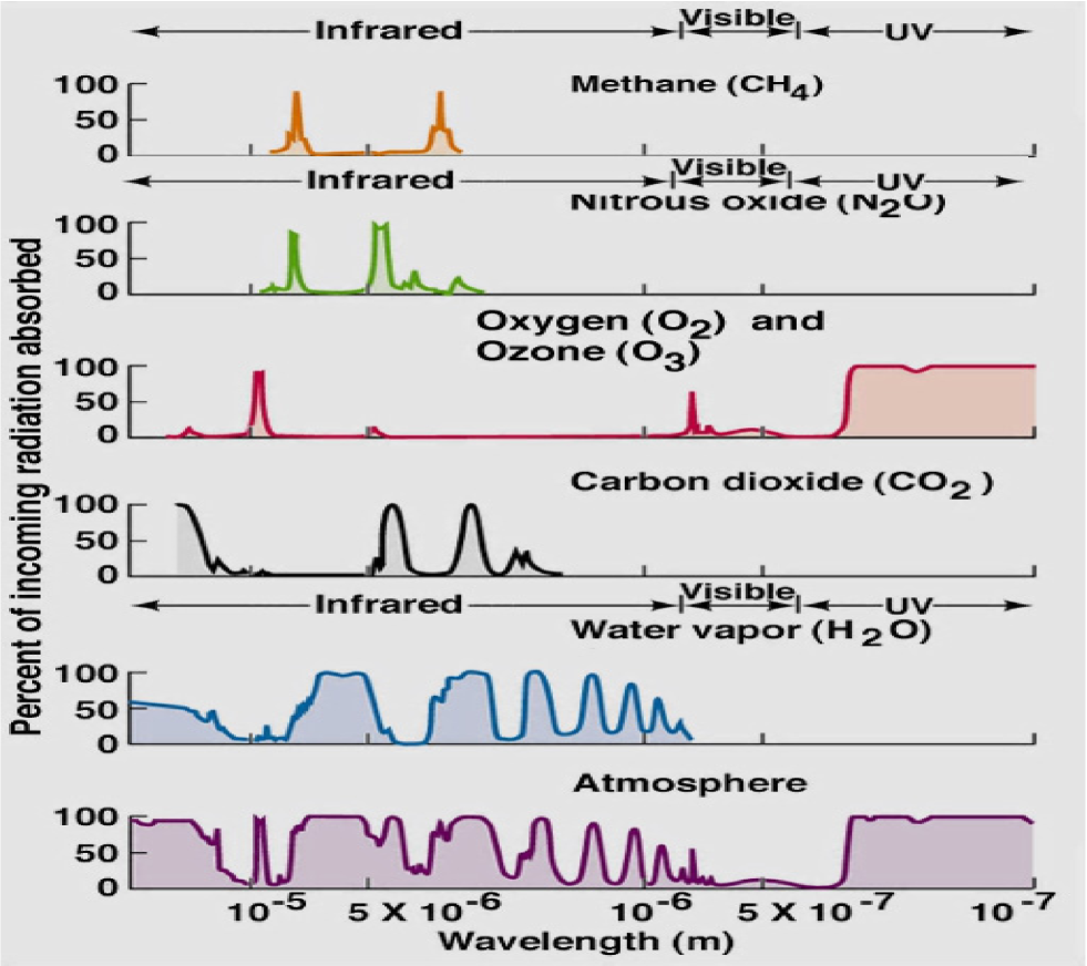
Figure 1: Absorption Spectra of some Trace Gases

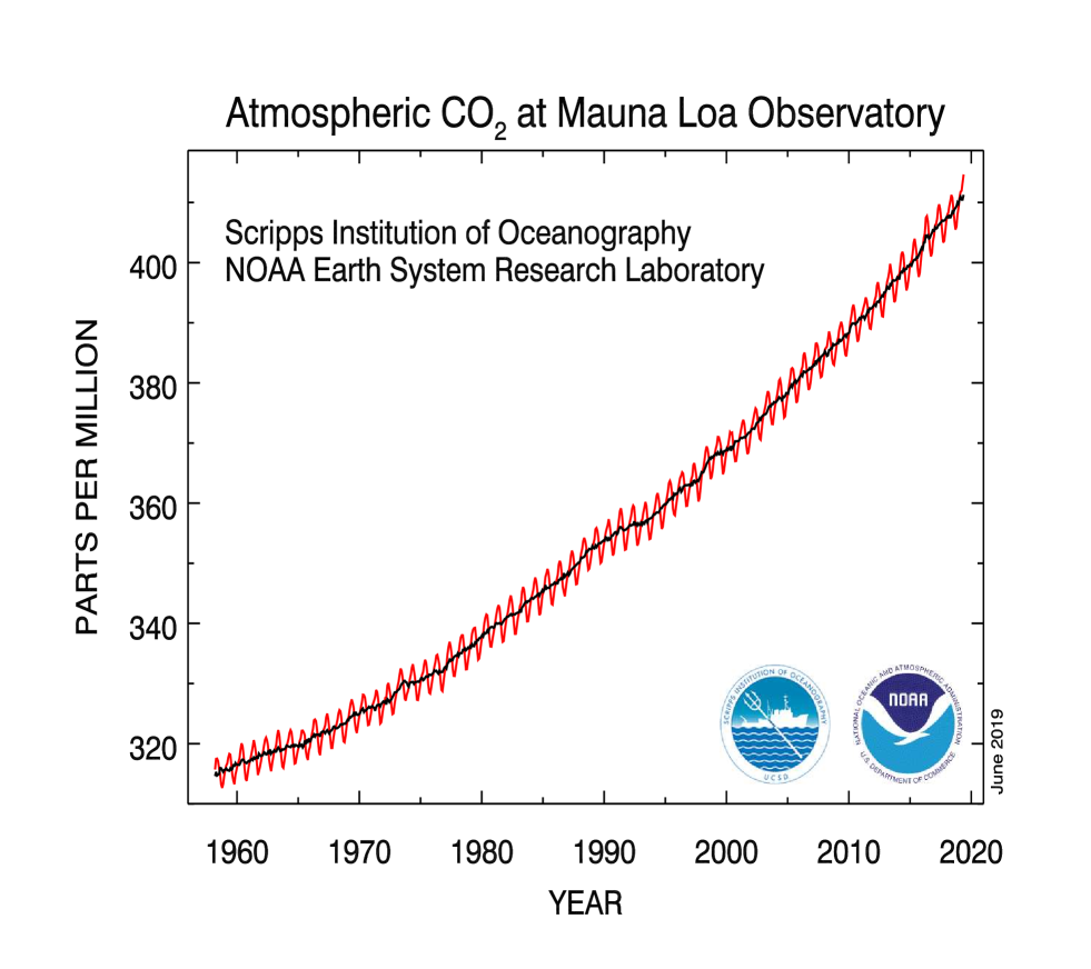
Figure 2:

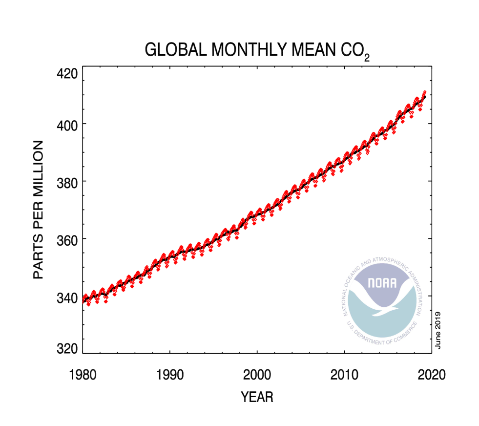
Figure 3:

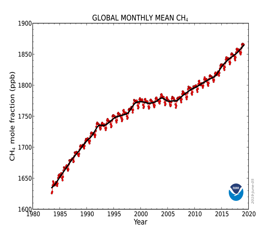
Figure 4:

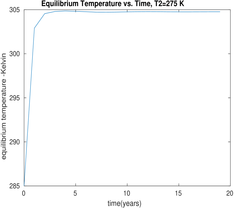
Figure 6:

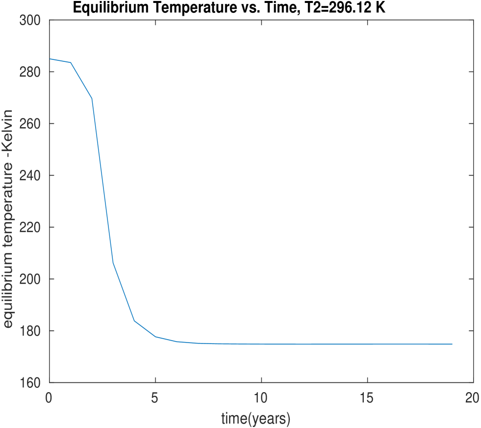
Figure 7:

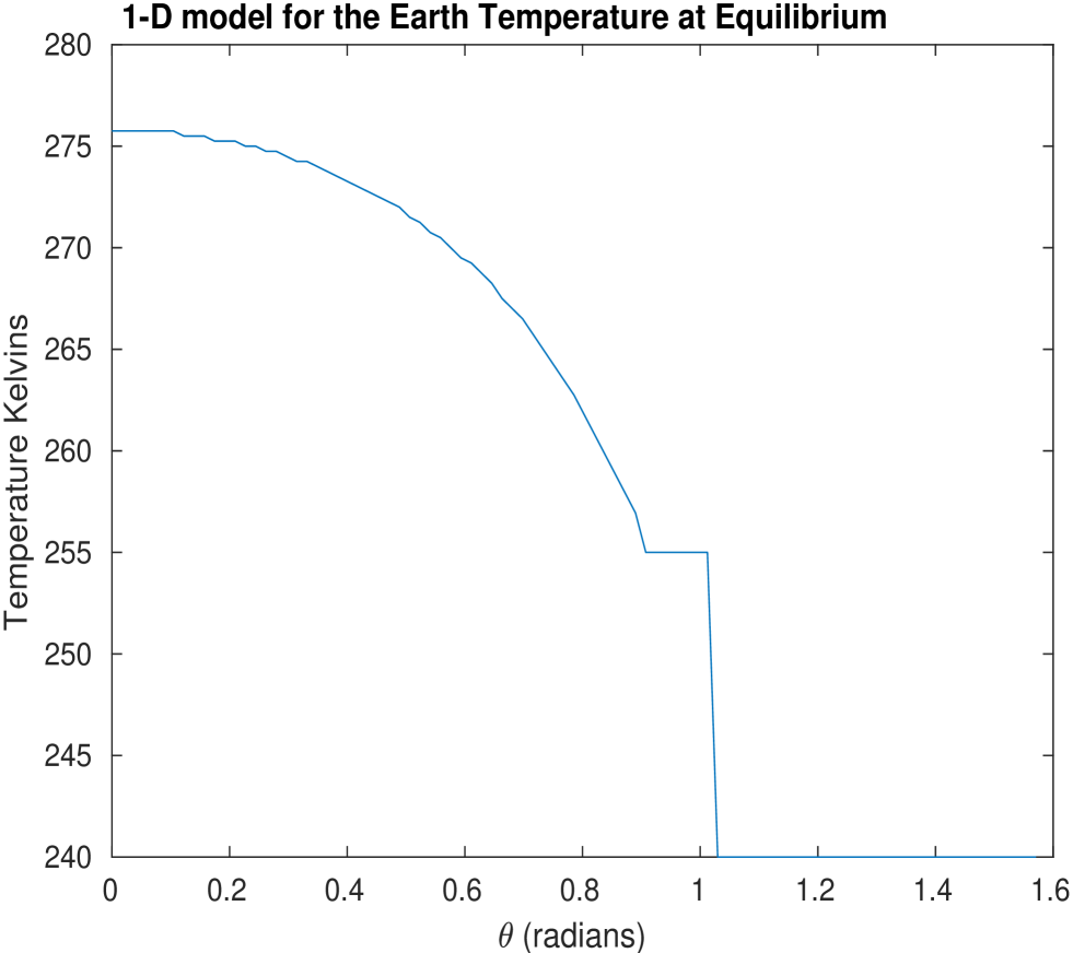
Figure 8:

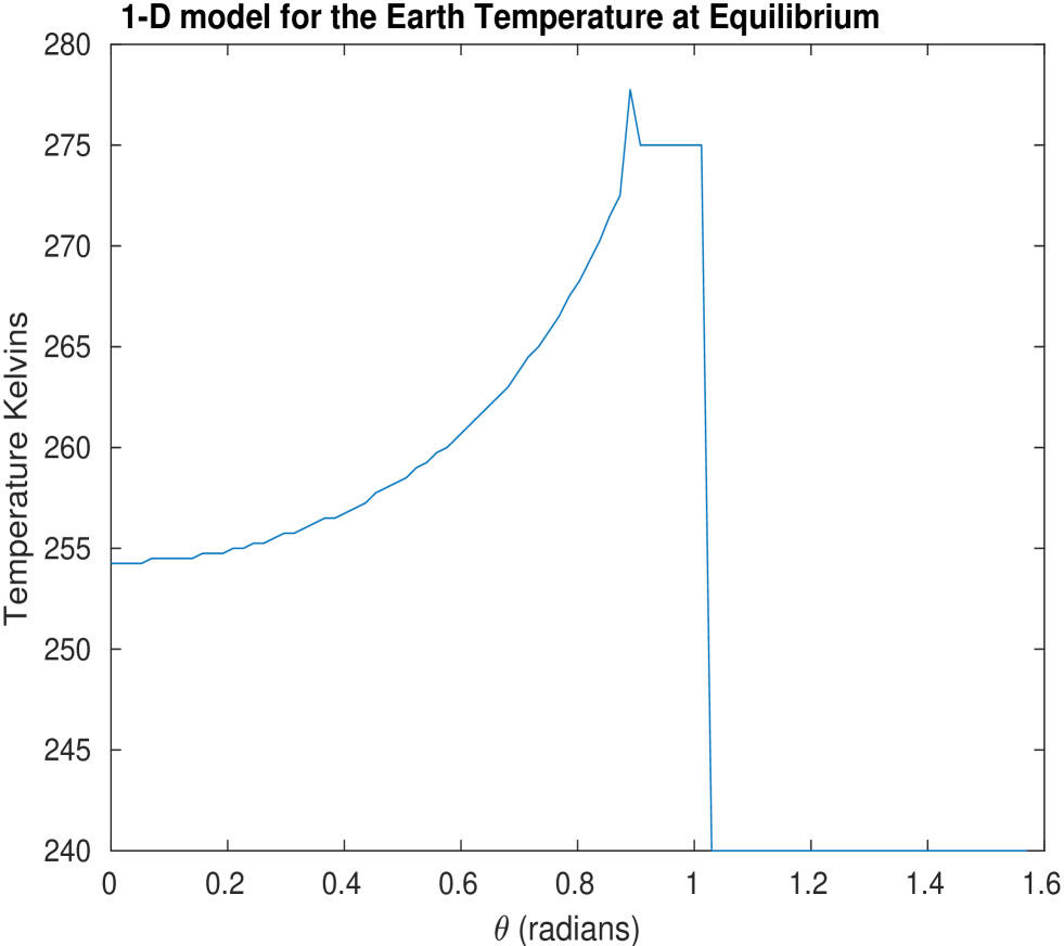
Figure 9:

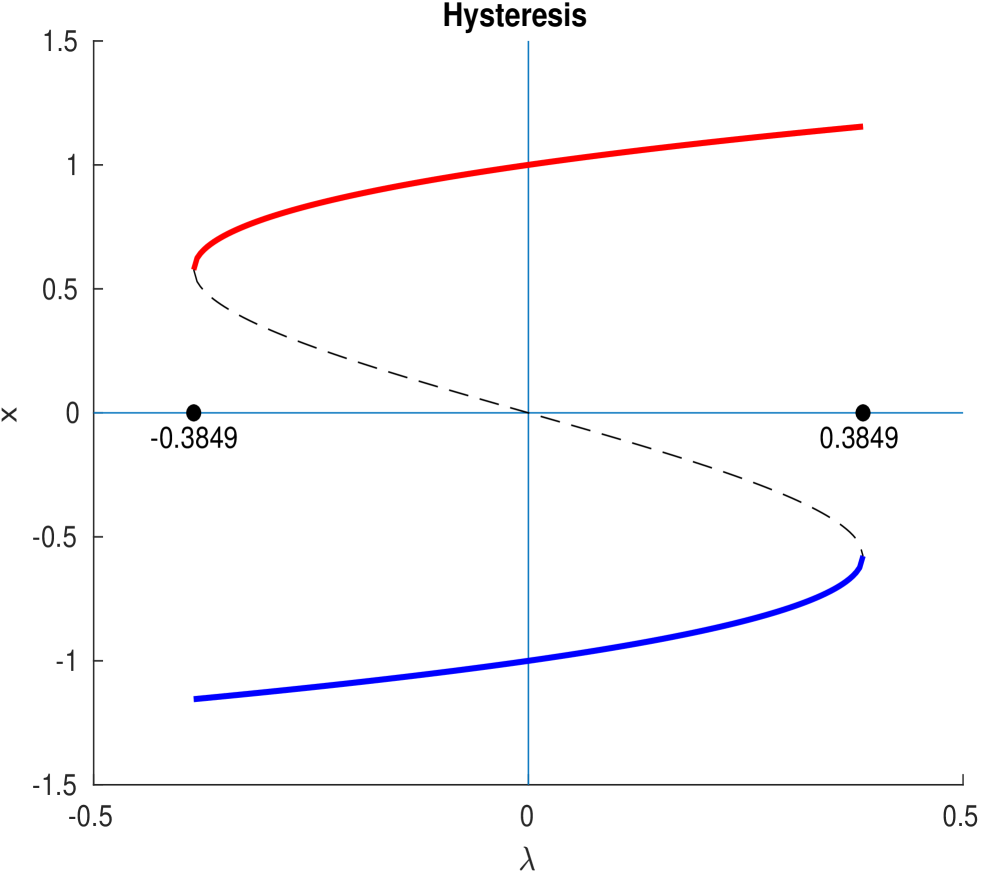
Figure 10:

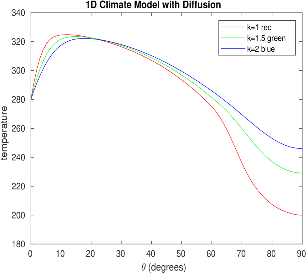
Figure 11:

References

- [1] W.D. Sellers -A climate model based on the Energy balance of the Earth-Atmosphere system, J. Appl. Met, 8, pp.392-400, 1969
- [2] W.D. Sellers - A New Global Climate Model, J. Appl. Met., 12, pp.241-254 ,1973
- [3] K. McGuffie and A.H. Sellers -A Climate Modeling Primer, Wiley, 3rd Ed. NY, 2005.
- [4] M. Ghil and S. Childress- Topic in Geophysical Fluid Dynamics, Chapter 10, Springer, NY. 1987.
- [5] D.J. Wilson, J. Gea-Banacloche - Simple model to estimate the contribution of atmospheric to the Earth’s greenhouse effect, Amer. J. Phys. Vol. 80, No. 4, pp. 306-315, 2012.
- [6] Dijkstra,H.A. -Numerical Bifurcation Methods applied to Climate Models: Analysis beyond Simulation, Preprint, Nonlin. processes in Geophysics., 2019.
- [7] https://www.esrl.noaa.gov/gmd/ccgg/trends/full.html.
- [8] https://www.esrl.noaa.gov/gmd/ccgg/trends/global.html.
- [9] https://www.esrl.noaa.gov/gmd/ccgg/trends/.
- [10] http://lasp.colorado.edu/home/sorce/data/tsi-data/.
- [11] https://geoengineering.environment.harvard.edu/geoengineering.
- [12] L. M. Russel et al, Bull. Am. Meteorological Soc., 94, pp. 709-729, 2013.
- [13] J. Tollefson - First sun-dimming experiment will test a way to cool Earth, Nature 563, pp. 613-615 ,2018.
- [14] S. M. Benson and D. R. Cole, Sequestration in Deep Sedimentary Formations, Elements, 4, pp. 325-331, 2008.
- [15] https://users.wpi.edu/ mhumi/model/.
- [16] O. Coddington, J.L. Lean, P. Pilewskie, M. Snow, D. Lindholm - A solar irradiance climate data record, Bull. American Meteorological Soc., 2015, doi: 10.1175/BAMS-D-14-00265.12.
- [17] G. Kopp and J. L. Lean - A new, lower value of total solar irradiance:Evidence and climate significance, Geophysical Research Letters VOL. 38, L01706, 2011, doi:10.1029/2010GL045777.