Numerical Optimization of Plasmid DNA Delivery Combined with Hyaluronidase Injection for Electroporation Protocol

Abstract

The definition of an innovative therapeutic protocol requires the fine tuning of all the involved operations in order to maximize the efficiency. In some cases, the price of the experiments, or their duration, represents a great obstacle and the full potential of the protocol risks to be reduced or even hidden by a non-optimal application.

The implementation of a numerical model of the protocol may represent the solution, allowing a systematic exploration of all the different alternatives, shedding the light on the most promising combination and also identifying the key elements/parameters.

In this paper, the injection of a plasmid, preceded by a hyaluronidase injection, is simulated through a mathematical model. Some key elements of the administration protocol are identified by means of a mathematical optimization procedure, maximizing the efficacy of the therapy. As a side effect of the extensive investigation, robust solutions able to reduce the effects of human errors in the administration are also obtained.

1 Introduction

DNA delivery consists in injecting engineered DNA plasmid vectors carrying nucleotide sequences coding therapeutic molecules, so that transfected cells can work as factory to produce locally or systematically specific products to correct pathological defects. It has a deep potential in revolutionizing therapeutic treatments in the field of infectious and cancer diseases, as demonstrated in past and recent studies [Wolff et al., 1990, André and Mir, 2004, Leguèbe et al., 2017]. However, DNA transfer is still very limited into the clinical practice: despite the treatment efficacy is well known, further improvements of delivery conditions are needed.

An important limitation to DNA transfection is represented by the transport of a plasmid through the Extra-Cellular Matrix (ECM) and its ability to cross the cell membrane and arriving into the cell nucleus for its expression [Grazia et al., 2014]. ECM consists of structural collagen network embedded in a gel of Glycosaminoglycans (GAGs) and proteoglycans, which prevents the free diffusion of macromolecules, such as plasmid vectors, and slows down the free diffusion of cytotoxic drugs, thanks also to the presence of degradation enzymes called nucleases [Bureau et al., 2004].

Lot of bioengineering strategies are under investigation for encompassing these barriers. One of them is the administration of hyaluronidase - an enzyme able to digest the ECM - before the DNA injection so improving the plasmid distribution within the injected tissue [Buhren et al., 2016, Girish and Kemparaju, 2007]. This methodology has been employed alone or in combination with electroporation (EP) [De Robertis et al., 2018]. The role of hyaluronidase in DNA immunization protocols by electroporation has been disscussed in [Chiarella et al., 2013a, Chiarella et al., 2013b, Chiarella and Signori, 2014].

EP consists in the application of electric fields to the cell membrane allowing its permeabilization to favor the DNA internalization [André and Mir, 2004, Aihara and Miyazaki, 1998, Rols et al., 1998]. Hyaluronidase treatment followed by EP of plasmid DNA, strongly improves the gene expression [McMahon et al., 2001, Akerstrom et al., 2015, Schertzer et al., 2006]. Although in [McMahon et al., 2001] differences in gene expressions due to time interval between intramuscular DNA injection and application of electric fields was briefly investigated, lot remains to be clarified.

Aim of this work is twofold: from one side, we need to identify the correct timing between hyaluronidase and DNA injection; as a second task, the effects of the waiting time between DNA injection and EP need to be evaluated and quantified. The use of numerical optimization algorithm, based on the results of the numerical simulation of the full process (apart from the EP itself), can help in the production of a large number of alternatives, restricting the range of variation of the single phases of the therapeutic protocol. The outcome of this study is the maximization of the effect of the therapy, here represented by the effective area reached by the therapeutic agent at the time of the application of the EP.

Paper is organized as follows: a section is devoted to the description of the mathematical model, previously introduced in [Deville et al., 2018]. Then, the numerical approach adopted for the determination of the most favorable conditions for the medical protocol are described, using metamodel interpolation, and the main results obtained by the optimization procedure are illustrated and discussed. The paper ends with some conclusions and future perspectives.

2 Model statement

In this section, we present the enzyme-based tissue degradation model proposed in [Deville et al., 2018]. The model combines the poroelastic theory of mixtures with the transport of enzymes and DNA plasmid densities in the extracellular space. The effect of the matrix degrading enzymes on the tissue composition and its mechanical response are also accounted for. The rationale of the model is schematically described in Figure 1.

Figure 1: Schematic description of exchange pathways and production terms of the different phases. From [Deville et al., 2018]

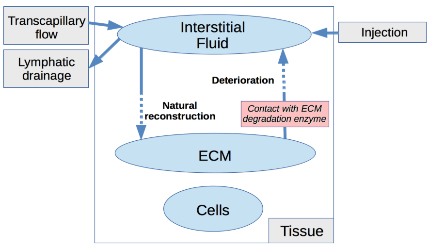
The governing equations are set in the fixed reference domain –the tissue at the initial time– denoted by $\Omega_{0}$. For the sake of simplicity, we assume that our system undergoes very small perturbations (see [Deville et al., 2018] for more details).

The poroelastic model of Deville et al. describes the behavior of the volume fractions of ECM, cells and fluid –namely the blood in the tissue– denoted respectively by $g_{\mathcal{E}}$, $g_{\text{\textcentoldstyle}}$ and $f$, as well as the evolution of the hyaluronidase concentration $h$ and the DNA concentration denoted by $c$. The displacement vector, due to fluid injection is denoted by ${\bf u}$, and $P$ is the inner pressure within the tissue.

The dimensionless model reads as

$$g_{\mathcal{E}}+g_{\text{\textcentoldstyle}}+f=1,$$ (1a)

$$\mbox{\boldmath$\nabla$}\cdot\left((g_{\mathcal{E}}+g_{\text{\textcentoldstyle}})\left(\overline{\lambda}(\nabla\cdot\textbf{u})I+\overline{\mu}(\nabla\textbf{u}+\nabla\textbf{u}^{T})\right)\right)=\nabla P,$$ (1b)

$$\begin{split}&(g_{\mathcal{E}}+g_{\text{\textcentoldstyle}})\overline{s_{0}}\frac{\partial P}{\partial t}-\nabla\cdot(\overline{\boldsymbol{\kappa}}\,\nabla P)=\alpha\,Q_{\scriptscriptstyle\mathrm{inj}}^{\scriptscriptstyle\mathrm{tot}}+\overline{\gamma}(\overline{P_{v}}-P)\\ &\hskip 42.67912pt+\left(\frac{\rho_{s}^{R,0}}{\rho_{f}^{R}}-1\right)g_{\mathcal{E}}(\overline{K}h+\overline{a_{r}}(f^{\rm phys}-f)),\end{split}$$ (1c)

$$\frac{\partial h}{\partial t}=\nabla\cdot(f\overline{\textbf{D}_{\scriptscriptstyle\mathrm{enz}}^{0}}\nabla h+hJ_{\scriptscriptstyle\mathrm{enz}})-\frac{\overline{k^{d}_{\scriptscriptstyle\mathrm{enz}}}}{f}h+\frac{\alpha\mathcal{S}_{\scriptscriptstyle\mathrm{enz}}}{c_{0}},$$ (1d)

$$\frac{\partial g_{\text{\textcentoldstyle}}}{\partial t}+\left(\overline{s_{0}}\frac{\partial P}{\partial t}\right)g_{\text{\textcentoldstyle}}=0,$$ (1e)

$$\frac{\partial g_{\mathcal{E}}}{\partial t}+\left(\overline{K}h+\overline{a_{r}}(f^{\rm phys}-f)+\overline{s_{0}}\frac{\partial P}{\partial t}\right)g_{\mathcal{E}}=0,$$ (1f)

$$\frac{\partial c}{\partial t}=\nabla\cdot(f\overline{\textbf{D}^{0}_{\scriptscriptstyle\mathrm{dna}}}\nabla c+cJ_{\scriptscriptstyle\mathrm{dna}})-\frac{\overline{k^{d}_{\scriptscriptstyle\mathrm{dna}}}}{f}c+\frac{\alpha\mathcal{S}_{\scriptscriptstyle\mathrm{dna}}}{c_{0}},$$ (1g)

where the fluxes of enzyme and DNA densities are defined by

$$J_{\scriptscriptstyle\mathrm{enz}}=\frac{1}{f}\overline{\boldsymbol{\kappa}}\,\nabla P-\overline{\textbf{D}_{\scriptscriptstyle\mathrm{enz}}^{0}}\nabla f\hskip 14.22636pt\text{ and }\hskip 14.22636ptJ_{\scriptscriptstyle\mathrm{dna}}=\frac{1}{f}\overline{\boldsymbol{\kappa}}\,\nabla P-\overline{\textbf{D}^{0}_{\scriptscriptstyle\mathrm{dna}}}\nabla f.$$ (2)

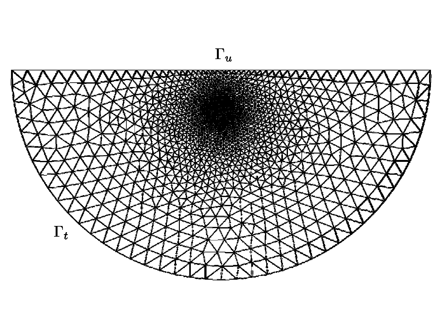
The above partial differential equations (PDEs) system is complemented with initial and boundary conditions. Denote by $\Gamma$ the boundary of the domain $\Omega_{0}$. We generically denote by n the normal to $\Omega$ outwardly directed from the inside to the outside of the domain. We suppose that $\Gamma$ is split into 2 parts denoted respectively by $\Gamma_{u}$ and $\Gamma_{t}$ (see Fig. 2). The following boundary conditions are imposed

$$\textbf{S}_{s}^{E}\,\mathbf{n}=0\text{ on }\Gamma_{t},\text{ and }\textbf{u}=0\text{ on }\Gamma_{u}$$ (3)

$$P=0\text{ on }\Gamma_{t}\text{ and }\nabla P\cdot\mathbf{n}=0\text{ on }\Gamma_{u},$$ (4)

$$h=0\text{ on }\Gamma_{t},$$ (5a)

$$\left(f\textbf{D}_{\scriptscriptstyle\mathrm{enz}}^{0}\nabla h+hJ_{\scriptscriptstyle\mathrm{enz}}\right)\cdot\textbf{n}=0\text{ on }\Gamma_{u}.$$ (5b)

The same type of boundary conditions are applied to the concentration of DNA plasmid and to its flux.

$$c=0\text{ on }\Gamma_{t},$$ (6a)

$$\left(f\textbf{D}^{0}_{\scriptscriptstyle\mathrm{dna}}\nabla c+cJ_{\scriptscriptstyle\mathrm{dna}}\right)\cdot\textbf{n}=0\text{ on }\Gamma_{u}.$$ (6b)

The initial conditions are given in Table 1.

We can observe from equation 6 how the PDEs system involves a large number of parameters. Being the model dimensionless, it is important to recall the link between the dimensionless (with a overline) and the physical (without overline) parameters as given in  [Deville et al., 2018]. We denote by $l_{0}$ the characteristic length of the tissue. The dimensionless Piola-Kirchhoff and Cauchy stress tensors are defined as $\overline{\textbf{S}^{E}_{s}}=\textbf{S}^{E}_{s}/(\lambda+2\mu)$ and $\overline{\boldsymbol{\sigma}^{E}_{s}}=\boldsymbol{\sigma}^{E}_{s}/(\lambda+2\mu)$, respectively, and we define the dimensionless parameters

$\displaystyle\overline{\mu}=\frac{\mu}{\lambda+2\mu}$,	$\displaystyle\overline{\lambda}=\frac{\lambda}{\lambda+2\mu}$,	$\displaystyle\overline{s_{0}}=s_{0}(\lambda+2\mu)$,	$\displaystyle\overline{\boldsymbol{\kappa}}=\frac{1}{\kappa}\boldsymbol{\kappa}$,
$\displaystyle\alpha=\frac{l_{0}^{2}}{\kappa(\lambda+2\mu)}$,	$\displaystyle\overline{K}=\alpha c_{0}K$,	$\displaystyle\overline{a_{r}}=\alpha a_{r}$,	$\displaystyle\overline{\gamma}=\frac{l_{0}^{2}}{\kappa}\gamma$,
$\displaystyle\overline{\textbf{D}_{\scriptscriptstyle\mathrm{enz}}^{0}}=\frac{1}{\kappa(\lambda+2\mu)}\textbf{D}_{\scriptscriptstyle\mathrm{enz}}^{0}$,	$\displaystyle\overline{k^{d}_{\scriptscriptstyle\mathrm{enz}}}=\alpha k^{d}_{\scriptscriptstyle\mathrm{enz}}$,	$\displaystyle\overline{P_{v}}=\frac{P_{v}}{\lambda+2\mu}$,
$\displaystyle\overline{\textbf{D}^{0}_{\scriptscriptstyle\mathrm{dna}}}=\frac{1}{\kappa(\lambda+2\mu)}\textbf{D}^{0}_{\scriptscriptstyle\mathrm{dna}}$,	$\displaystyle\overline{k^{d}_{\scriptscriptstyle\mathrm{dna}}}=\alpha k^{d}_{\scriptscriptstyle\mathrm{dna}}$.

We choose the $(\lambda+2\mu)$ parameter as a natural pressure scale; by this choice the dimensionless elastic parameters $\overline{\lambda},\overline{\mu}$ are of order $1$ [Lang et al., 2016]. Some of the physical parameters can be found in the literature, and others depend on the experimental protocol. The physical parameters that are considered fixed are given in Table 1, where, if nothing is reported, correspond to the values proposed [Deville et al., 2018].

The aforementioned systems of equations have been numerically solved by adopting the finite element method: the practical implementation has been obtained by using the open-source libraries FreeFEM [Hecht, 2012]. Details are provided in [Deville et al., 2018].

Table 1: Values of the physical parameters fixed for the numerical parametric studies, see also [Deville et al., 2018].

Parameter	Symbol	Value	Unit	Reference
Typical length	$l_{0}$	$10^{-2}$	m
Reference concentration	$c_{0}$	$10^{9}$	kg/$\text{m}^{3}$
Density of fluid phase	$\rho^{R}_{f}$	$10^{3}$	kg/$\text{m}^{3}$	[Yao et al., 2012]
Density of solid phase	$\rho^{R,0}_{s}$	$1.09\times 10^{3}$	kg/$\text{m}^{3}$	[Ward and Lieber, 2005]
Specific storage coefficient	${s_{0}}$	$10^{-6}$	$\text{Pa}^{-1}$
Injected concentration	$c_{\scriptscriptstyle\mathrm{inj}}^{\scriptscriptstyle\mathrm{enz}}$	$4\times 10^{-2}$	U/$\mu$l	[McMahon et al., 2001]
Permeability	${\boldsymbol{\kappa}}$	$10^{-11}$	$\text{m}^{2}\text{Pa}^{-1}\text{s}^{-1}$	[Swartz and Fleury, 2007]
Lamé first parameter	${\lambda}$	$7.14\times 10^{5}$	Pa	[Zöllner et al., 2012]
Lamé second parameter	${\mu}$	$1.79\times 10^{5}$	Pa	[Zöllner et al., 2012]
Diffusion coefficient of the enzyme	${\textbf{D}^{0}_{\scriptscriptstyle\mathrm{enz}}}$	$10^{-4}$	$\text{m}^{2}$/s
Diffusion coefficient of the therapeutic agent	${\textbf{D}^{0}_{\scriptscriptstyle\mathrm{dna}}}$	$10^{-9}$	$\text{m}^{2}$/s
Starling’s coefficient	${\gamma}$	$5\times 10^{-5}$	$\text{Pa}^{-1}\text{s}^{-1}$	[Soltani and Chen, 2012]
Fluid/solute coefficient	$\gamma_{c}$	$0.9$	-	[Baxter and Jain, 1989]
Measure of treatment efficacy	${K}$	$10^{-14}$	$\text{m}^{3}\text{s}^{-1}\text{U}^{-1}$
Recovery coefficient	${a_{r}}$	$5\times 10^{-4}$	$\text{s}^{-1}$
Degradation rate of the enzyme	${k^{d}_{\scriptscriptstyle\mathrm{enz}}}$	$1\times 10^{-4}$	$\text{s}^{-1}$
Degradation rate of the therapeutic agent	${k^{d}_{\scriptscriptstyle\mathrm{dna}}}$	$2\times 10^{-4}$	$\text{s}^{-1}$
Driving pressure	${P_{v}}$	$10^{-1}$	Pa
Initial values	Symbol	Initial value	Unit
Volume fraction of fluid	$\varphi_{f}(0,\textbf{x})=\varphi^{\rm phys}_{f}$	$0.1$	-
Volume fraction of ECM	$\varphi_{\mathcal{E}}(0,\textbf{x})$	$0.4$	-
Volume fraction of cells	$\varphi_{\text{\textcentoldstyle}}(0,\textbf{x})$	$0.5$	-
Network dilatation	$\nabla\cdot\textbf{u}(0,\textbf{x})$	$0$	-
Enzyme concentration	$h(0,\textbf{x})$	$0$	$\text{Um}^{-3}$
DNA concentration	$c(0,\textbf{x})$	$0$	$\text{Um}^{-3}$
Initial pressure	$p(0,\textbf{x})$	$0$	Pa

3 Parametric investigation and optimization

A mathematical model, describing the different phases of the dosing regimen, represents a strong and powerful tool for the determination of the correct execution of the different actions to be taken during the administration protocol. In particular, starting form the analysis produced in [Deville, 2017], we have observed how some parameters are not optimally selected, although they appears to be able to change deeply the final effect of the whole procedure. Some experimental trials have been produced in order to drive the selection of the best values, but the number of attempts is clearly limited by the costs of the experimental activity, and the final result can be reasonably further improved. Under this perspective, the use of a mathematical model would be of great aid.

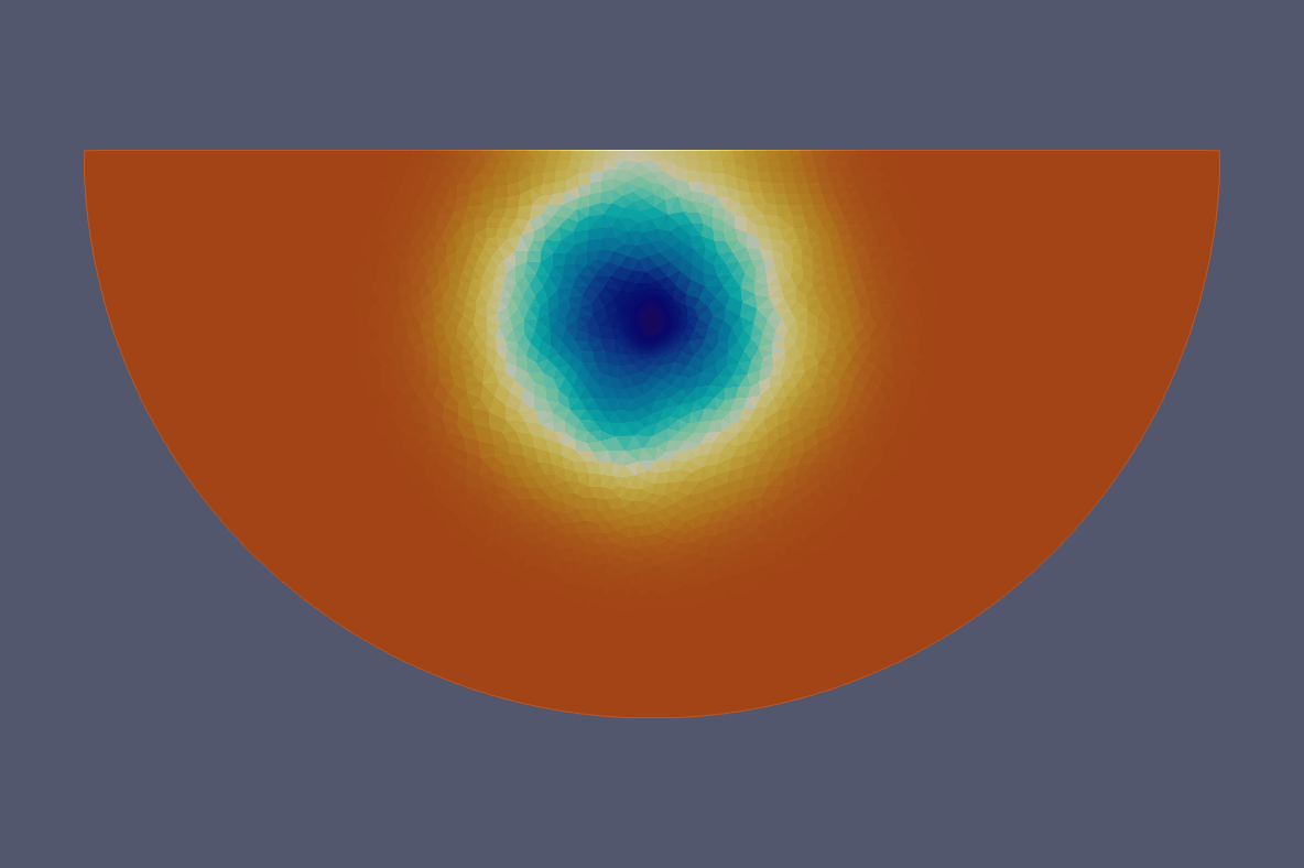
The numerical simulation of the effects of the complete dosing regimen is obtained by discretizing a portion of the tissue where the injections will be performed and observing the diffusion of the plasmid and the DNA in this volume, resolving the previously described systems of equations. In figure 2, an example of the computational mesh is reported. The problem is solved numerically under the assumption of spherical symmetry: for this reason, the solution of a two-dimensional representation of the tissue is sufficient. In the picture, the semi-circular area represents a planar section of an half-sphere. The upper border (planar) represents the skin surface, while the semi-circular area represents a portion of the tissue under the skin surface. The diffusion of the therapeutic agents is observed into this volume.

Figure 2: Computational grid for the current problem: the density of the cells is increased in the area around the injection point.

3.1 Selection of relevant parameters

In order to find the best value of the different parameters, they can be systematically changed: a number of different configurations are numerically evaluated with the aim of detecting the best strategy for the dosing of the therapy. To do that, we have to define a criterion for the quantification of the preference of a configuration with respect to another: reasonably, we can assume the maximum value of the volume occupied by the DNA during the time as a measure of the effectiveness of the combination of parameters. Considering that a minimal quantity of the plasmid is required in order to be effective, we can assume the area where the concentration of the plasmid is higher than a minimum value as the effective area. Since a deterioration of the plasmid is observed in time, the effective area is typically growing during the injection phase and in the successive moments, but after a certain time (depending on the administration strategy) it is decreasing. With the mathematical model we are able to take trace of this evolution, determining its maximum value and the time at which it occurs, including also the evolution of the effective area after the maximum value has reached. The plasmid is here considered as effective when it represents at a concentration of 5% or more: this check is performed on every cell adopted in the discretization of the investigated volume, and the area of every active cell is contributing to the full effective area.

Figure 3: Evolution of the area reached by the therapeutic agent during the time starting from the end of the plasmid injection.

Among the different elements of the dosing regimen, we put our attention on the sequence of the injections. Here we can observe four different phases:

• Hyaluronidase injection.

• Waiting time for the hyaluronidase diffusion into the tissue.

• Plasmid injection.

• Waiting time for the plasmid diffusion into the tissue.

For each injection, there are some undetermined quantities:

• The duration of the injection phase.

• The amount of the injected substance.

• Deepness of the injection.

The injected quantities of hyaluronidase and plasmid have been fixed at $25\mu\,l$ and $30\mu\,l$ respectively, and the deepness of the injections have been assumed to be the same for both. After these choices, we have still four free parameters:

1. Duration of the hyaluronidase injection $T_{Hy}$ .

2. Waiting time for the hyaluronidase diffusion into the tissue $\Delta_{T}$ .

3. Duration of the plasmid injection $T_{DNA}$ .

4. Deepness of injections $D_{inj}$ .

These four parameters have been adopted, in the following, as the design parameters whose best value is searched.

3.2 Features of the mathematical model

The determination of the optimal values of the four parameters requires, in general, the application of an optimization algorithm: once a mathematical programming problem is formulated, a large number of trial vectors of the design parameters need to be automatically generated and evaluated, as soon as the convergence to the optimal values of the parameters is obtained. Unfortunately, the numerical noise connected with the numerical solution of the problem and the large computational time required to finalize a single simulation represent two great obstacles in the application of this approach. In fact, a noisy behavior of the function to be minimized/maximized is typically creating a number of false minima/maxima, and the optimization algorithm is sometime trapped into those regions. Regarding the CPU time for the solution of a single configuration, depending on the values of the parameters, it could be greater than five hours, and around ten thousand of simulation are needed for reaching the convergence to the optimal solution in our case.

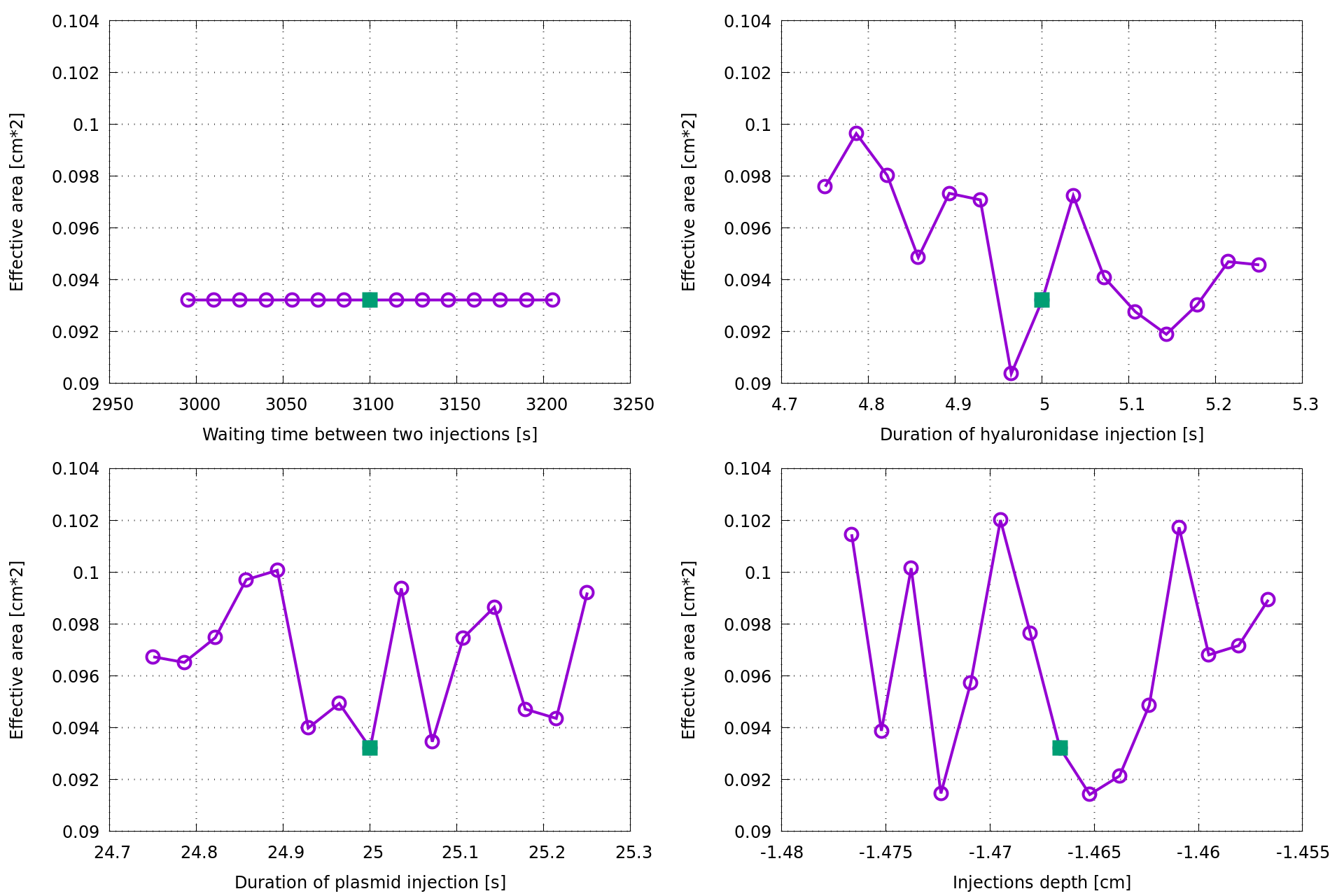
An example of the effects of the numerical noise is reported in figure 4. Here a very small variation of a single parameter is enforced, while all the other parameters are kept fixed. The effect of the variation of a single parameter on the total effective area is reported in the corresponding sub-figure. The central value is representing one of the best configuration identified during the following exploration. We can observe how, in the investigated region, the time between the two injections is not changing at all the value of the effective area, while for the other parameters a nearly random effect is observed: it is evident that a sort of uncertainty is connected with the estimate of the effective area, and the simple punctual value provided by the simulation cannot be representative of the real effects of the selected parameters. For this reason, we should try to define a different value of the effective area, able to put into consideration the strong local sensitivity to the parameters of the output of the simulations. We decided here to apply a worst case approach, and the average value of a group of local samples, reduced by the associated variance, is defined as our objective function. Statistically, the use of this quantity guarantees that the effective area in the neighborhood of the selected configuration of the dosing parameters is greater than the indicated value with a probability of 84.15%. For this reason, from now on we will refer to the effective area as its average value (computed on a sampling set of 9 configurations) minus the variance.

Figure 4: Sensitivity analysis of the area reached by the therapeutic agent as a function of the injection deepness only. On the left, comparison between the point values and the interpolated ones, on the right the interpolated values only (scales are different).

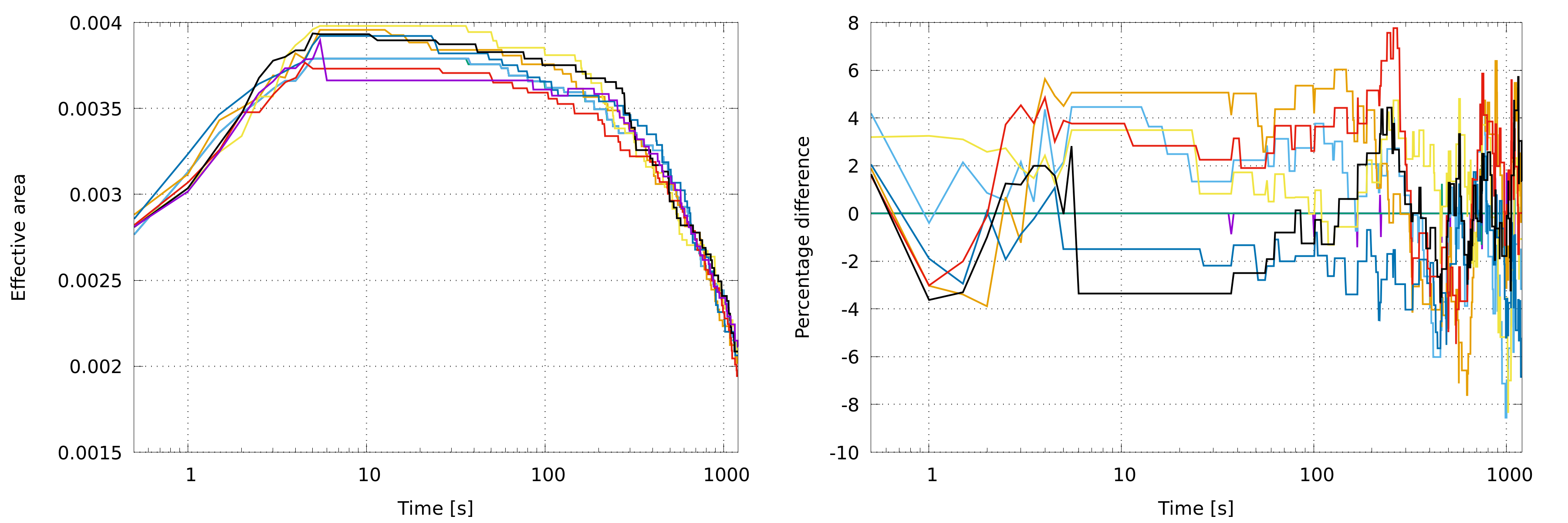
In figure 5 we have reported the full evolution curve of the effective area for the nine configurations adopted during the sensitivity analysis of a single simulated point. On left, the differences in absolute terms are reported, on the right the percentage differences are shown. Percentage differences are computed with respect to the value of the central point of the distribution. We can observe how a difference of about eight percentage points is recorded among the different curves: this represents a sign of great sensitivity of the simulation model to the parameter variation. The fluctuations are slightly amplified by the lower value of the effective area at the end of the curve: anyway, this behavior represents a strong element for the consideration of an averaged value instead of a punctual value of the effective area.

Figure 5: Absolute (left) and percentage (right) differences observed on the nine configurations adopted in the sensitivity analysis. Percentage differences are computed with respect to the central point of the distribution.

Another aspect that we should take into consideration, and that advises against the use of an optimization algorithm, is that the practical implementation of the prescription includes human errors, so that the precision of the effectively realized parameters is practically low. As a consequence, we are much more interested in some general indications about the order of magnitude of the various parameters rather than an extremely precise list of values for our parameters. Human errors can be reduced by a partial or even complete automation of the different operation, however some steps should be necessarily performed manually, in particular when a living creature is involved in the application.

3.3 Selection of the optimization strategy

On the base of the previous considerations, the strategy adopted in this paper is based on the general framework of the ”Multipoint Approximation Method” [Toropov, 1995], or, more in general, of the ”Metamodel-Based Simulation Optimization” (see [Barthelemy and Haftka, 1993, Barton and Meckesheimer, 2006]). This approach can be synthetically described as follows. The first step consists in the generation of a suitable number of training points, preferably regularly spaced, spanning the design variable space. The number of the training points is unknown a priori, depending typically on the rate of variation of the objective function and on the number of design variables. It can be fixed also considering the allowed computational effort for the optimization activities. The objective function is now computed at the training points, obtaining the so called training set. The training set is used in order to derive an interpolation/approximation of the objective function over the full design space, generally called metamodel (a model of the model). The metamodel is substantially an algebraic model, able to mimic the numerical response of the computationally expensive mathematical model. The training phase of the metamodel depends on the characteristics of the metamodel itself: during the training phase, the parameters of the metamodel are optimized in order to minimize the prevision error. Some metamodels are trained easily, i.e. by solving a linear system whose dimension is equal to the number of training points, other metamodels require the solution of an optimization algorithm (like neural networks). A small part of the training set can be put momentarily aside, forming the verification set, and then it can be used at the end of the training phase in order to verify the accuracy of the metamodel on positions not previously used during the training. Several techniques can be now adopted in order to select new training points with the aim of increasing the accuracy of the prediction, if required: examples are reported in [Peri, 2009, Shu et al., 2017]. Once the quality of the metamodel is satisfactory, it can be applied to the optimization algorithm, in order to identify the optimal parameters of the mathematical model. Since the evaluation of the metamodel is computationally inexpensive if compared with the mathematical model, the overall computational cost of the optimization procedure is equal to the time of the training phase.

3.4 Details of the optimization strategy

In this application, we selected the Orthogonal Arrays [Hedayat et al., 1999](OA) for the generation of the training set. OA represents a reduced set with respect to the full factorial design obtained by a regular sampling of each coordinate direction: some configurations are deleted from the full factorial design, and the remaining ones are respecting an orthogonality criteria. In this case, 16 levels for the regular subdivision of each direction of the design space have been selected: a complete full factorial design is composed by 65536 points, here reduced to 512 sampling points after the application of the OA criterion. Since we need to perform a sensitivity analysis for each sample point, the total number of configurations to be analyzed is 4608.

As a surrogate model, a multi-dimensional spline approximator [Peri, 2018] has been adopted, tuned using the results provided by the previously produced training set. The interval of variation for the parameters has been fixed as follows: $\Delta_{T}$ is varied between 300 and 10800 seconds; $T_{Hy}$ and $T_{DNA}$ are varied between 5 and 30 seconds, and $D_{inj}$ is varied between 1 and 2 centimeters. These values have been selected observing previous numerical experiences from [Deville, 2017].

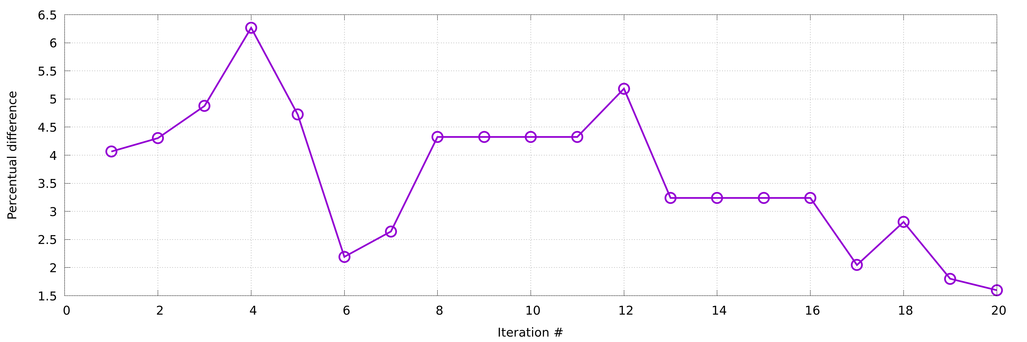
In order to increase the credibility of the meta-model, some further training points have been added sequentially in those areas where the objective function appears to be favorable. The full number of training points, at the end of the refinement phase, has become 686 (6174 configurations). A solution of mathematical model is produced for the new training points, and the difference between the value of the objective function estimated by the meta-model and the real value provided by the mathematical model at the new point is assumed as the precision index of the meta-model. The history of the refinement phase is reported in figure 6. Range of variations of the parameters are also adjusted.

Figure 6: Precision index of the meta-model during the refinement phase.

The determination of the best configuration is obtained by regularly sampling the design space and then recursively refining the investigation as soon as the dimension of the investigated area is lower than a prescribed limit. Since this operation is completed by using the metamodel, we can adopt very strict parameters: we have here 51 subdivision along each coordinate direction and the final spatial precision of the search is fixed at $10^{-8}$.

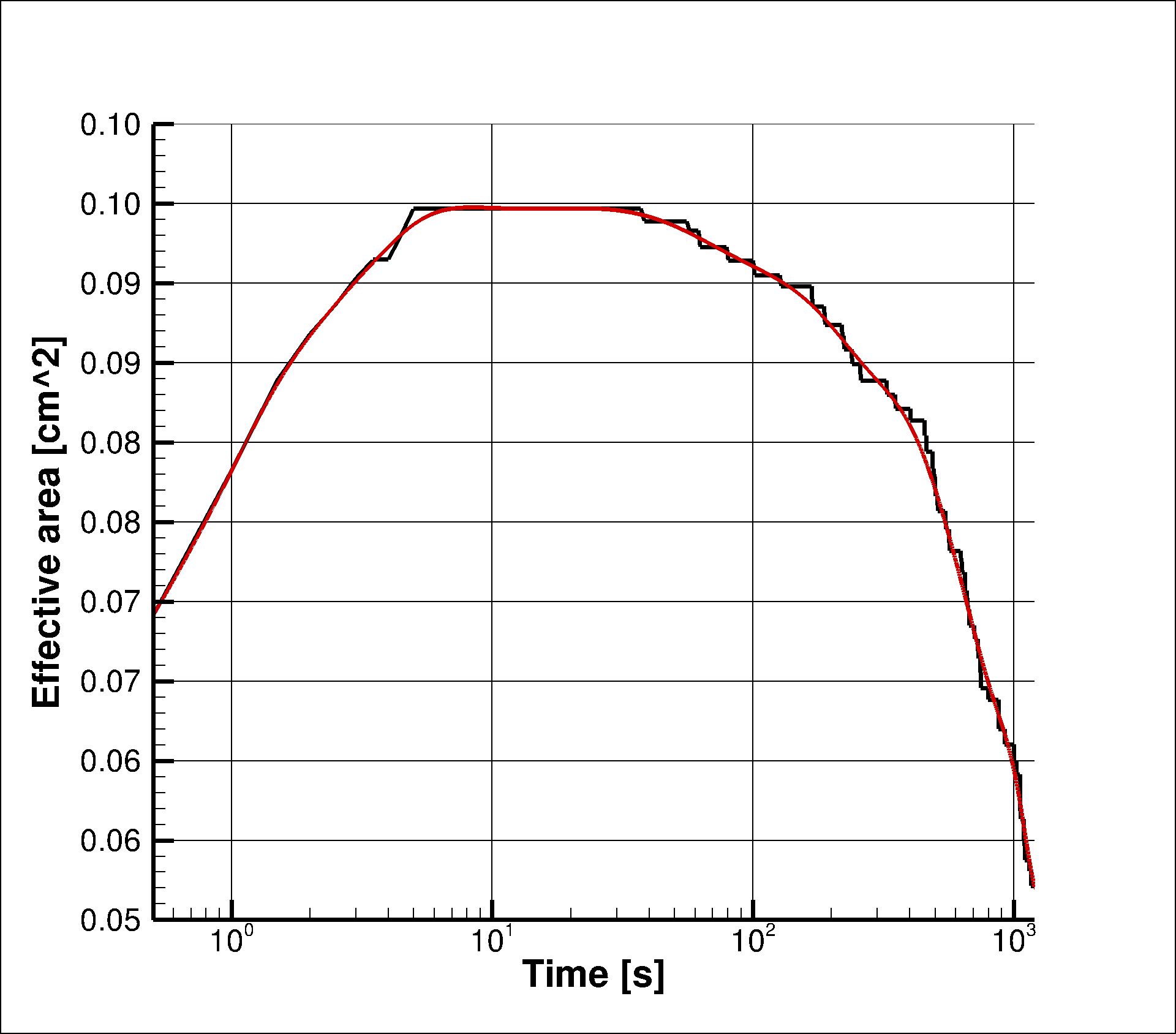
3.5 Results

So far, the maximum value of the effective area have been considered. We can observe in picture 3 that the best value is typically obtained after ten seconds from the end of the plasmid injection, and this value is nearly constant for about 30 seconds: this is in line with the practical necessities of the preparation of the following EP (normally form 10 to 20 seconds). Since after that time the effective area is reducing, if the waiting time for the EP is longer than 30-40 seconds we have a loss of efficiency of the full prescription. In order to estimate the degradation of the effective area in time, 5 different pictures have been produced at 1, 2, 4, 8 and 16 minutes after the end of the plasmid injection. In this case, the value of the objective function is reported, so that following pictures are showing the average of the effective area reduced by their variance. Since we need to take into consideration the inaccurate realization of the parameters, in the pictures a dot is reported only if the objective function is at least greater than 99% of the maximum observed value of the objective function: this way, we have a representation of the areas of the parameter space where we can substantially guarantee the maximum efficiency of the prescription, reducing the negative effects of a small error of the implementation. Results are reported for different values of the depth, that is fixed in each sub-picture at the indicated value, and for two different waiting time before EP, that is, 1 and 16 minutes.

Figure 7: Range of parameters for which a loss of 1% with respect to the maximum realizable effective area is obtained. Time after the plasmid injection completion: 1 minute.

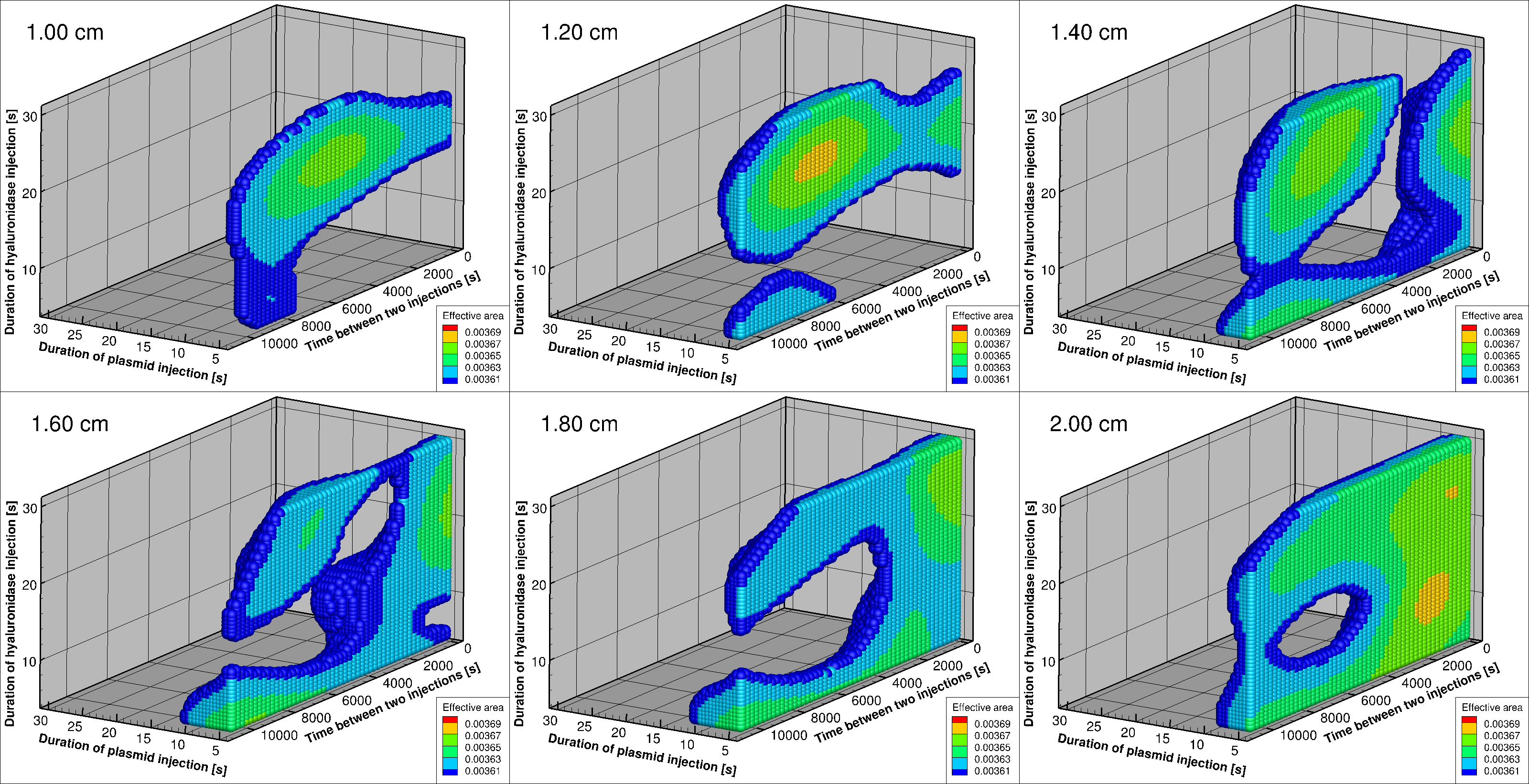
If we are able to complete the preparation of the EP phase in 1 minute, the duration of the plasmid injection should be very small. From figure 7 we can observe how the preferable value of $D_{inj}$ is not univocal, since similar values are obtained for 1.2 centimeters and 2 centimeters, but the values of $\Delta_{T}$ are different, being shorter in the case of the deeper injection. This may represents an advantage if a series of experiments are performed.

Figure 8: Range of parameters for which a loss of 1% with respect to the maximum realizable effective area is obtained. Time after the plasmid injection completion: 16 minutes.

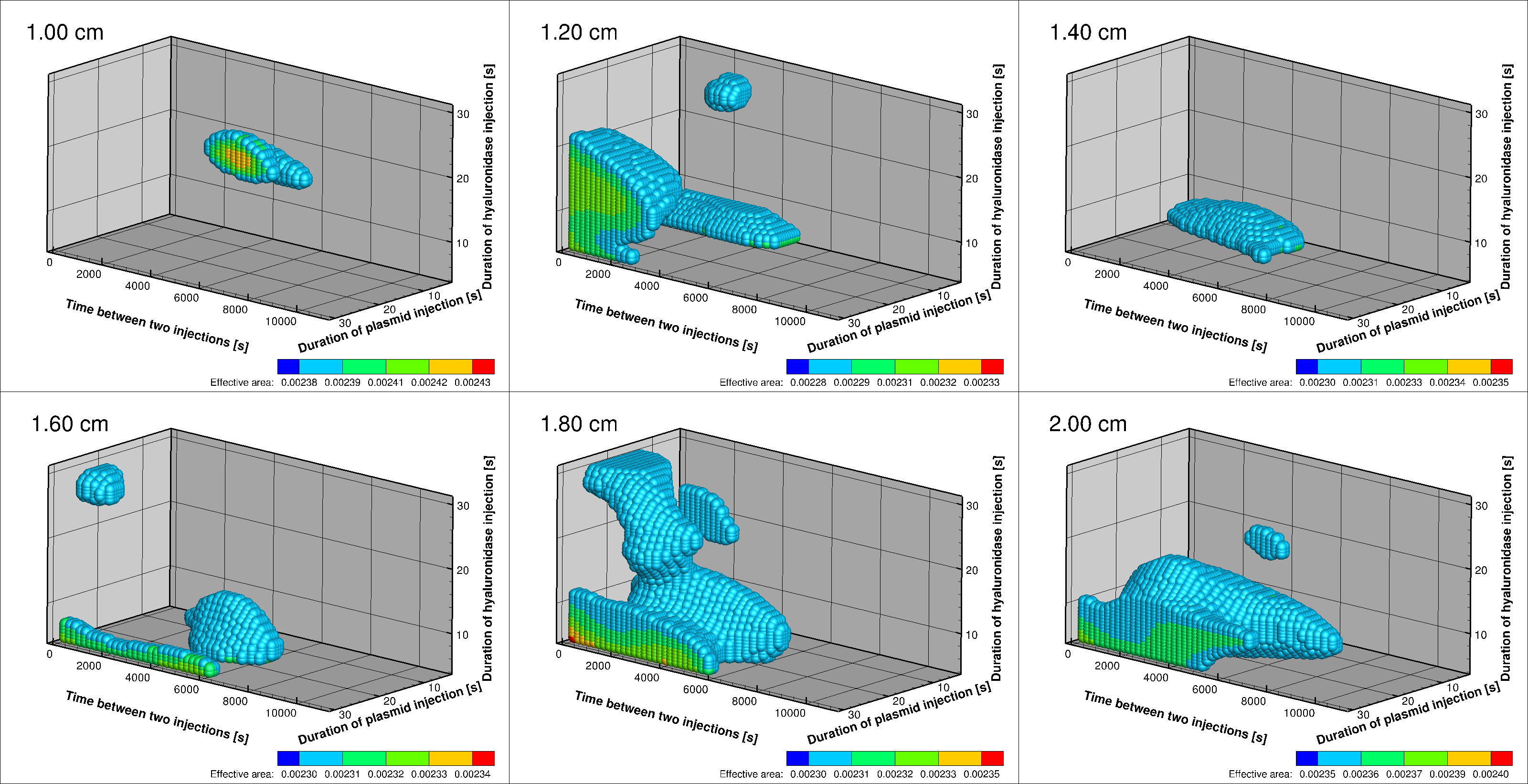
On the contrary, if we observe the results after 16 minutes, reported in figure 8, the value of the objective function for the case of $D_{inj}$ equal to 2 centimeters is larger than in the other cases. $T_{DNA}$ can be longer, while $\Delta_{T}$ is variable.

If we now fix $D_{inj}$ at 2 centimeters, we can observe the effect of $\Delta_{T}$ , reported in figure 9. The scale of the objective function is changing from sub-picture to sub-picture.

Figure 9: Range of parameters for which a loss of 1% with respect to the maximum realizable effective area is obtained. Depth of the injections: 2 centimeters.

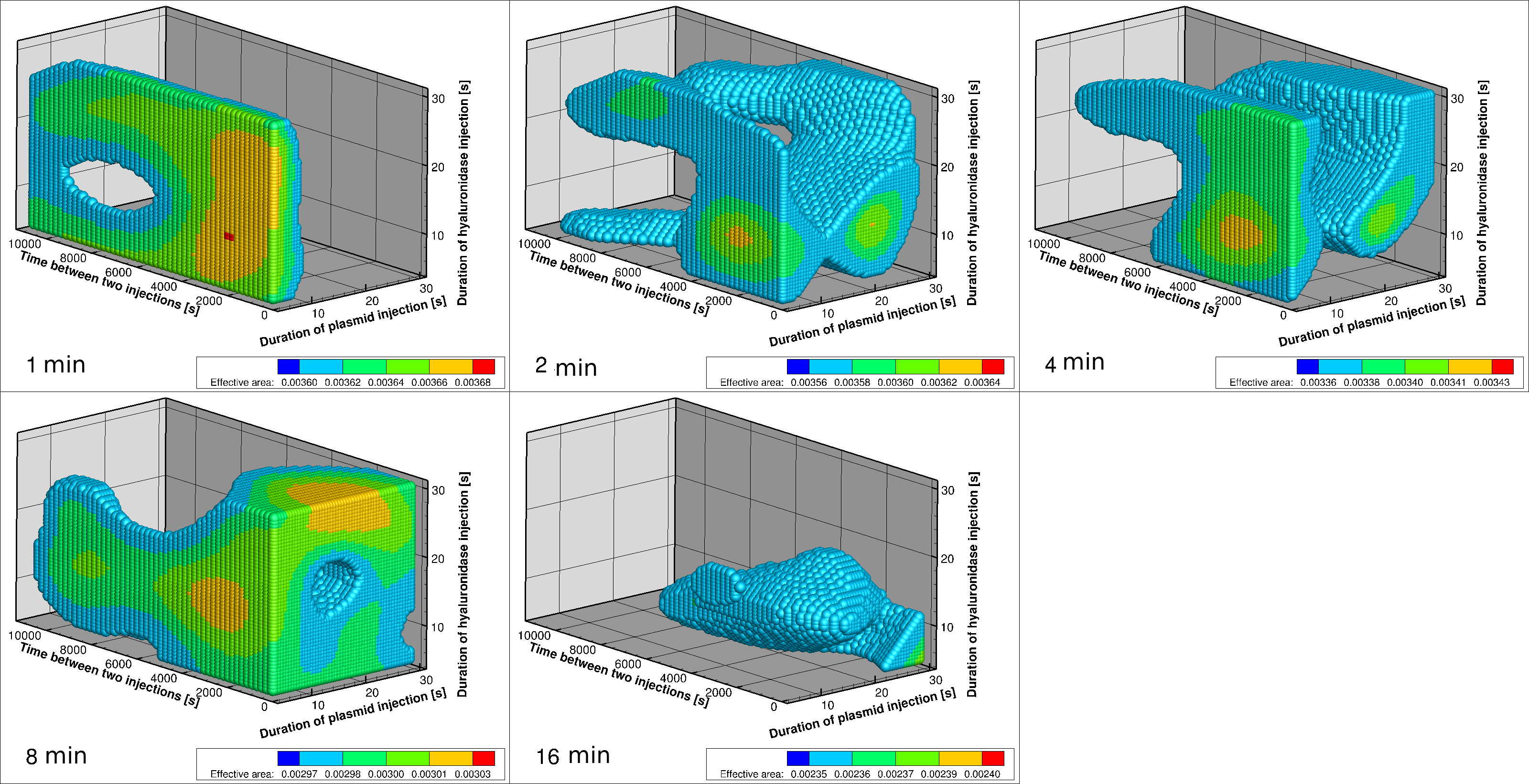
After 8 minutes we have the larger tolerance in the best parameters: this area is largely reduced if the EP is performed after 16 minutes. At the same time, the objective function is reduced if the EP waiting time is increased. The numerical estimate of this loss is reported in figure 10.

Figure 10: Loss in the effective area with an increasing $\Delta_{T}$ . On top, absolute values. On bottom, percentage values.

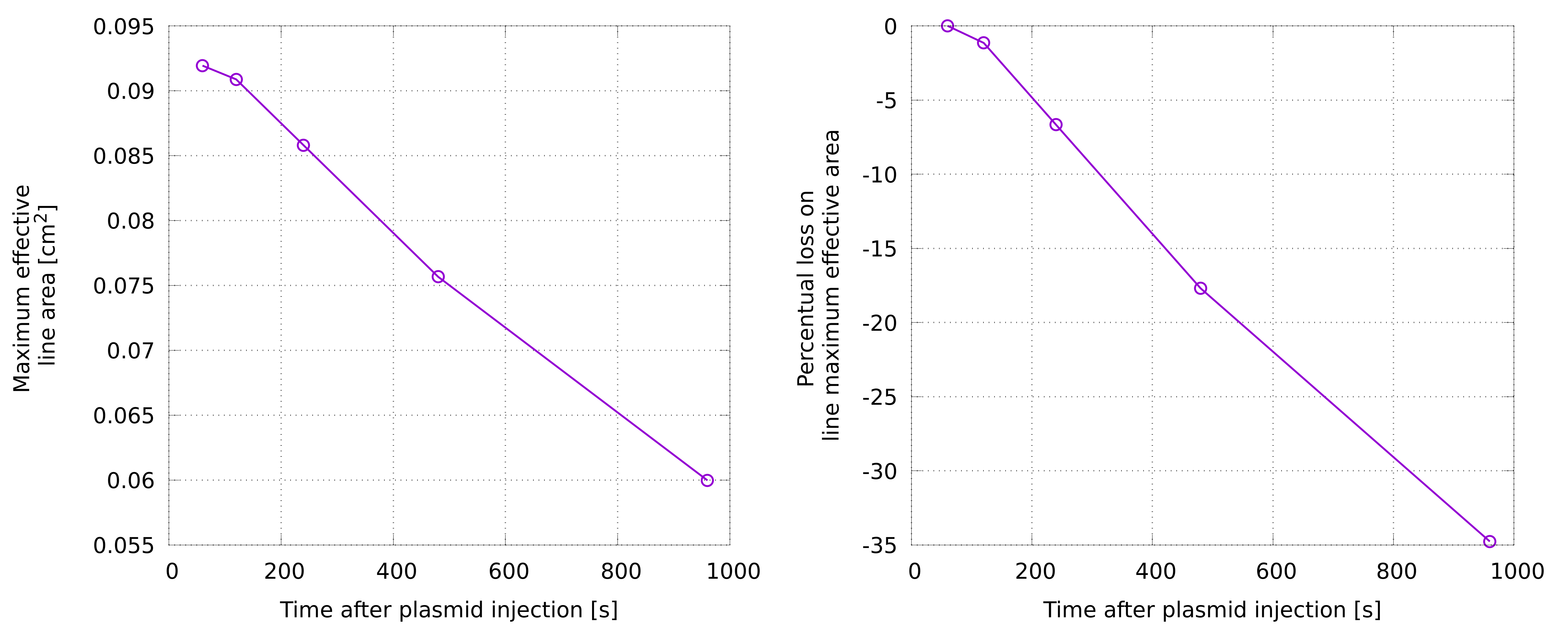
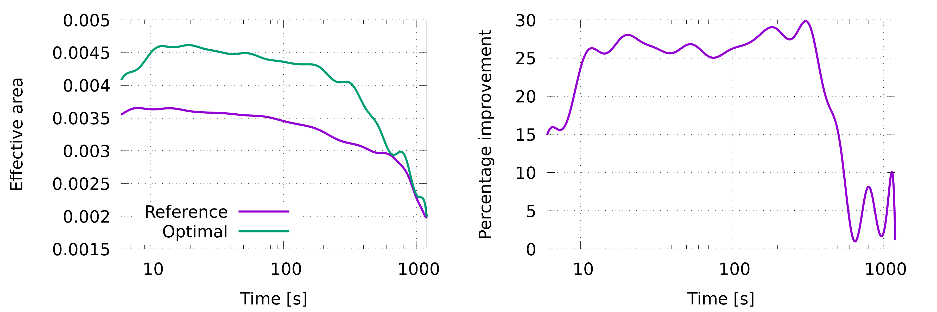
In order to quantify the improvements potentially obtained by the optimization procedure, a reference configuration, commonly adopted for this kind of experiments, has been compared with the best configuration identified by the optimization procedure. Results are reported in figure 11. An increase of about 30% is obtained if the EP is performed after no more then 8 minutes from the DNA injection: in fact, it is obviously convenient to perform the EP at the moment of the maximum expansion of the DNA into the tissues. If the waiting time is greater than 10 minutes, the two different strategies does not show significant differences, probably because the dynamics connected with the degradation of the DNA are substantially independent from the protocol details. The observation of these results suggest not to delay the EP procedure after 30 seconds: this request may require the application of a fully automated operations, in order to reduce the time spent in all the different preliminary sub-activities required by EP, such as correct immobilization of the subject undergoing to EP, application of conductive gel in the area to treat, correct placement of the electrodes, etc.). This time reduction is of paramount importance since a longer waiting time is almost nullifying all the advantages obtained by the optimized protocol.

Figure 11: Comparison between a reference configuration and the overall optimal configuration identified by the numerical analysis.

3.6 Role of $T_{DNA}$ 

In the common practice, a quite long waiting time between the two injections, hyaluronidase and DNA, is adopted. Typically, $T_{DNA}$ is about one or two hours later respect to the hyaluronidase administration. This assumption has been motivated by the necessity to be sure that the hyaluronidase has enough time to develop its effect, increasing the porosity of the ECM and then facilitating the access of the DNA-plasmid at the border of the cells.

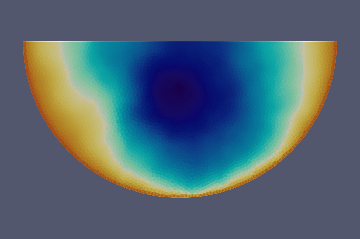
At the end of the solution of the optimization process, two categories of best solutions have been identified: the overall best configuration ever computed in terms of effective area and the best configuration in terms of objective function. The second solution is the preferable one, since it takes into account the variability of the effective area under small variations of the control parameters. The set of realized parameters differs largely between the two solutions: in particular, while in the first case $\Delta_{T}$ is 3500 seconds, in the second case $\Delta_{T}$ is nearly 300 seconds. This second option is absolutely preferable, since it reduces a lot the overall execution time of the experiment, but a deeper analysis is needed in order to understand why different timings led to similar results. In figure 12, the elements for a reasonable explanation are reported. In the picture, we have plotted the porosity of the tissue at the time of the DNA-plasmid injection for the two different values of $\Delta_{T}$ . In the same picture, the maximum expansion of the DNA-plasmid in the tissue is also reported, plotting the area in which the concentration of DNA-plasmid is more than 5%. We can observe how the effect of the hyaluronidase is clearly increasing with $\Delta_{T}$ , since almost the whole computational volume has been interested by the action of the hyaluronidase when $\Delta_{T}$ is 3500 seconds.

For the shorter value of $\Delta_{T}$ , the same effect is obtained in the very central part of the computational volume, but the effect vanishes quickly. On the bottom part of figure 12, the area in which we have a significant concentration of DNA-plasmid is reported: we can observe how this area is really small, so that the effect of the hyaluronidase in the case of the small $\Delta_{T}$ is absolutely sufficient.

This result is connected with the large dimensions of the DNA-plasmid, and consequently its great difficulties in traveling into the ECM. Observing this result, we can argue that multiple injections of DNA-plasmid in a small area could probably increase (linearly with the number of injection sites) the overall effect of the protocol, since further modifications of the method of administration of the hyaluronidase appear not to be effective.

In table 2, the exact values of the design parameters are reported for three different options for the protocol: the reference values ($\alpha$), based on some indications about common practice adopted in pre-clinical protocols, the configuration providing the best overall value of the effective area ($\beta$) and the configuration maximizing the objective function ($\gamma$). Since the objective function is taking into account the stability of the solution in the neighborhood of the computational point, this last configuration is preferable. We can observe that, in the case $\alpha$ we have the maximum values for $\Delta_{T}$ and $D_{inj}$ , while $T_{Hy}$ and $T_{DNA}$ are the smaller ones. Both $\beta$ and $\gamma$ suggest a smaller value of $\Delta_{T}$ , significantly shorter in the case $\gamma$. This is probably the more interesting result, since this allows for a huge compression of the overall duration of the experiment and gives also some indications about the behavior of the DNA-plasmid. $T_{Hy}$ and $T_{DNA}$ are larger for both $\beta$ and $\gamma$ with respect to $\alpha$: due to the small injected quantities, probably the implementing rules suggested in $\beta$ cannot be practically achieved. The smaller value of $D_{inj}$ in $\beta$ and $\gamma$, on the contrary, is compatible with the experimental setup.

Figure 12: On top: Porosity variation in the computational domain at the corresponding $\Delta_{T}$ . On left, $\Delta_{T}$ is 3800 seconds, on right is about 290 seconds. On bottom, the maximum area where the concentration of the DNA-plasmid is larger than 5%.

Table 2: Values of the control parameters for three different configuration of the protocol: reference values (current common practice), best effective area (punctual value), best objective function value (locally averaged value).

Parameter	Reference	Best EA	Best OF
$T_{Hy}$ [cm]	2.00	1.47	1.52
$\Delta_{T}$ [s]	10.00	28.33	21.47
$T_{DNA}$ [s]	5400.00	3800.00	289.60
$D_{inj}$ [s]	10.00	9.98	14.54

4 Conclusions

Improvements of gene electrotranfer protocol are becoming of paramount importance to translate this treatment into human patients. When DNA plasmid vector is injected into tissues, its expression is limited, due to the presence of ECM and cell membrane barriers. The employment of hyaluronidase, which allows a partial digestion of the ECM, and EP - a physical methodology favoring cell membrane permeabilization - represents a valid platform for DNA delivery expression. In this study, a mathematical model simulating the core part of the delivery protocol has been applied in order to enhance the DNA expression, identifying the best injection and waiting time for the DNA administration. Once numerically compared with the standard operative protocol, the optimal strategy returns an improvement of about 30% on the DNA delivery expression. This encouraging result is subject to the capacity of maintain the waiting time between the DNA injection and the application of EP inside a maximum of 200 seconds.

A dedicated experimental in vivo protocol will be hopefully performed in order to validate the numerical results: this would also be a decisive aid in the transfer of this medical approach from labs to everyday clinics.

References

- [Aihara and Miyazaki, 1998] Aihara, H. and Miyazaki, J.-i. (1998). Gene transfer into muscle by electroporation in vivo. Nature Biotechnology, 16:867–870.
- [Akerstrom et al., 2015] Akerstrom, T., Vedel, K., Needham, J., and Hojman, P. (2015). Optimizing hyaluronidase dose and plasmid DNA delivery greatly improves gene electrotransfer efficiency in rat skeletal muscle. Biochemistry and Biophysics Reports.
- [André and Mir, 2004] André, F. M. and Mir, L. M. (2004). Dna electrotransfer: its principles and an updated review of its therapeutic applications. Gene therapy, 11 Suppl 1:S33–42.
- [Barthelemy and Haftka, 1993] Barthelemy, J. F. M. and Haftka, R. T. (1993). Approximation concepts for optimum structural design - a review. Structural optimization, 5(3):129–144.
- [Barton and Meckesheimer, 2006] Barton, R. R. and Meckesheimer, M. (2006). Chapter 18 metamodel-based simulation optimization. In Henderson, S. G. and Nelson, B. L., editors, Simulation, volume 13 of Handbooks in Operations Research and Management Science, pages 535 – 574. Elsevier.
- [Baxter and Jain, 1989] Baxter, L. T. and Jain, R. K. (1989). Transport of fluid and macromolecules in tumors. i. role of interstitial pressure and convection. Microvascular research.
- [Buhren et al., 2016] Buhren, B. A., Schrumpf, H., Hoff, N.-P., Bölke, E., Hilton, S., and Gerber, P. A. (2016). Hyaluronidase: from clinical applications to molecular and cellular mechanisms. European journal of medical research, 21(1):5.
- [Bureau et al., 2004] Bureau, M. F., Naimi, S., Ibad, T. R., and Seguin, J. (2004). Intramuscular plasmid dna electrotransfer: biodistribution and degradation. Biochimica et Biophysica Acta (BBA).
- [Chiarella et al., 2013a] Chiarella, P., De Santis, S., Fazio, V. M., and Signori, E. (2013a). Hyaluronidase contributes to early inflammatory events induced by electrotransfer in mouse skeletal muscle. Human Gene Therapy, 24(4):406–416.
- [Chiarella et al., 2013b] Chiarella, P., Fazio, V. M., and Signori, E. (2013b). Electroporation in dna vaccination protocols against cancer. Current Drug Metabolism, 14(3):291–299.
- [Chiarella and Signori, 2014] Chiarella, P. and Signori, E. (2014). Intramuscular dna vaccination protocols mediated by electric fields. Electroporation Protocols, 1121:315–324.
- [De Robertis et al., 2018] De Robertis, M., Pasquet, L., Loiacono, L., Bellard, E., Messina, L., Vaccaro, S., Di Pasquale, R., Fazio, V. M., Rols, M.-P., Teissi’e, J., Golzio, M., and Signori, E. (2018). In vivo evaluation of a new recombinant hyaluronidase to improve gene electro-transfer protocols for dna-based drug delivery against cancer. Cancers, 10(11):1–20.
- [Deville, 2017] Deville, M. (2017). Mathematical mode of enhanced grug deliery by mean of electroporation or enzymatic treatment. PhD thesis, Université de Bordeaux & Università di Roma Tor Vergata.
- [Deville et al., 2018] Deville, M., Natalini, R., and Poignard, C. (2018). A continuum mechanics model of enzyme-based tissue degradation in cancer therapies. Bulletin of Mathematical Biology, 80(12):3184–3226.
- [Girish and Kemparaju, 2007] Girish, K. S. and Kemparaju, K. (2007). The magic glue hyaluronan and its eraser hyaluronidase: a biological overview. Life sciences, 80(21):1921–1943.
- [Grazia et al., 2014] Grazia, N. M., Roberto, N., and Emanuela, S. (2014). Gene therapy: the role of cytoskeleton in gene transfer studies based on biology and mathematics. Current Gene Therapy, 14(2):121–127.
- [Hecht, 2012] Hecht, F. (2012). New development in freefem++. Journal of Numerical Mathematics, 20(3-4):251–265.
- [Hedayat et al., 1999] Hedayat, A. S., Sloane, N. J. A., and Stufken, J. (1999). Orthogonal Arrays: Theory and Applications. Springer-Verlag, New York.
- [Lang et al., 2016] Lang, G. E., Vella, D., Waters, S. L., and Goriely, A. (2016). Mathematical modelling of blood-brain barrier failure and oedema. Mathematical medicine and biology : a journal of the IMA.
- [Leguèbe et al., 2017] Leguèbe, M., Notarangelo, M. G., Twarogowska, M., Natalini, R., and Clair, P. (2017). Mathematical model for transport of dna plasmids from the external medium up to the nucleus by electroporation. Mathematical Biosciences, 285(Supplement C):1 – 13.
- [McMahon et al., 2001] McMahon, J. M., Signori, E., Wells, K. E., Fazio, V. M., and Wells, D. J. (2001). Optimisation of electrotransfer of plasmid into skeletal muscle by pretreatment with hyaluronidase - increased expression with reduced muscle damage. Gene Therapy, 8:1264–1270.
- [Peri, 2009] Peri, D. (2009). Self-learning metamodels for optimization. Ship Technology Research, 56(3):95–109.
- [Peri, 2018] Peri, D. (2018). Easy-to-implement multidimensional spline interpolation with application to ship design optimisation. Ship Technology Research, 65(1):32–46.
- [Rols et al., 1998] Rols, M., Delteil, C., Golzio, M., Dumond, P., Cros, S., and J, T. (1998). In vivo electrically mediated protein and gene transfer in murine melanoma. Nature Biotechnology, 16(2):168–171.
- [Schertzer et al., 2006] Schertzer, J. D., Plant, D. R., and Lynch, G. S. (2006). Optimizing plasmid-based gene transfer for investigating skeletal muscle structure and function. Molecular Therapy, 13(4).
- [Shu et al., 2017] Shu, L., Jiang, P., Wan, L., Zhou, Q., Shao, X., and Zhang, Y. (2017). Metamodel-based design optimization employing a novel sequential sampling strategy. Engineering Computations, 34(8):2547–2564.
- [Soltani and Chen, 2012] Soltani, M. and Chen, P. (2012). Effect of tumor shape and size on drug delivery to solid tumors. Journal of biological engineering.
- [Swartz and Fleury, 2007] Swartz, M. A. and Fleury, M. E. (2007). Interstitial flow and its effects in soft tissues. Annual review of biomedical engineering, 9:229–256.
- [Toropov, 1995] Toropov, V. V. (1995). Multipoint Approximation Method for Structural Optimization Problems with Noisy Function Values, pages 109–122. Springer Berlin Heidelberg, Berlin, Heidelberg.
- [Ward and Lieber, 2005] Ward, S. R. and Lieber, R. L. (2005). Density and hydration of fresh and fixed human skeletal muscle. Journal of biomechanics, 38(11):2317–2320.
- [Wolff et al., 1990] Wolff, J. A., Malone, R. W., Williams, P., Chong, W., Acsadi, G., Jani, A., and Felgner, P. L. (1990). Direct gene transfer into mouse muscle in vivo. Science (New York, N.Y.), 247(4949 Pt 1):1465–1468.
- [Yao et al., 2012] Yao, W., Li, Y., and Ding, G. (2012). Interstitial fluid flow: the mechanical environment of cells and foundation of meridians. Evidence-based complementary and alternative medicine : eCAM, 2012:853516.
- [Zöllner et al., 2012] Zöllner, A. M., Abilez, O. J., Böl, M., and Kuhl, E. (2012). Stretching skeletal muscle: chronic muscle lengthening through sarcomerogenesis. PloS one, 7(10):e45661.