Grammatical Sequence Prediction for
Real-Time Neural Semantic Parsing

Abstract

While sequence-to-sequence (seq2seq) models achieve state-of-the-art performance in many natural language processing tasks, they can be too slow for real-time applications. One performance bottleneck is predicting the most likely next token over a large vocabulary; methods to circumvent this bottleneck are a current research topic. We focus specifically on using seq2seq models for semantic parsing, where we observe that grammars often exist which specify valid formal representations of utterance semantics. By developing a generic approach for restricting the predictions of a seq2seq model to grammatically permissible continuations, we arrive at a widely applicable technique for speeding up semantic parsing. The technique leads to a 74% speed-up on an in-house dataset with a large vocabulary, compared to the same neural model without grammatical restrictions.

1 Introduction

Executable semantic parsing is the task of mapping an utterance to a logical form (LF) that can be executed against a data store (such as a SQL database or a knowledge graph), or interpreted by a computer program in some other way. Various authors have tackled this task via sequence-to-sequence (seq2seq) models, which have already led to substantial advances in machine translation. These models learn to directly map the input utterance into a linearised representation of the corresponding LF, predicting it token by token. Seq2seq approaches have yielded state-of-the-art accuracy on both classic (e.g., Geoquery Zelle and Mooney (1996) and Atis Dahl et al. (1994)) and more recent semantic parsing datasets (e.g., WebQuestions, WikiSQL and Spider) Liang et al. (2017); Dong and Lapata (2016, 2018); Yin and Neubig (2018); Yu et al. (2018). The recent datasets are of much larger scale, which not only enables the use of more data-hungry models, such as deep neural networks, but also provides more complex challenges for semantic parsing.

The material presented in this paper was motivated by a question-answering dataset for equity search in a financial data and analytics system. We will refer to this dataset as “the EQS dataset” going forward (and we will refer to “equity search” as EQS for short). The queries in the dataset pertain to equity stocks; they are usually of the form Show me companies that satisfy such-and-such criteria, or What are the top 10 companies that $\cdots$?, and so on. The dataset pairs such queries with logical forms that capture their semantics. These logical forms are designed to be readily translatable into an executable query language in order to retrieve the corresponding answers from a data store in the back end. Questions can involve a large number of diverse search criteria, such as price, earnings per share, country of domicile, membership in indices, trading in specific exchanges, etc., applied to a large set of equities for which the system offers information.

The large number of search criteria and entities is reflected in the LFs, leading to a problem common with newer, more complex semantic-parsing datasets: having to deal with a large LF vocabulary size. In the EQS dataset the LF vocabulary has a size that exceeds 50,000. Since seq2seq models apply some operation over the whole vocabulary – usually the softmax operation – when deciding what symbol to output next, large LF vocabularies can slow them down considerably. For example, we observe in our EQS experiments with seq2seq models that it takes on average between 250 and 300 milliseconds to parse a query, which is too slow for one single component in a larger, real-time question-answering pipeline. This is consistent with observations made previously in the neural language modelling literature; see for example Bengio et al. (2003); Mikolov et al. (2010), where the authors show that when the vocabulary size exceeds a certain threshold, the softmax calculation becomes the computational bottleneck.

Our proposal for tackling this bottleneck is based on the fact that there generally exist grammars, which we call LF grammars, specifying the concrete syntax of valid logical forms (LFs). This is usually the case because LFs need to be machine-readable. We further note that, for a given LF prefix, one can usually use the LF grammar to look up the next grammatically permissible tokens (i.e., tokens that are part of a grammatically valid completion of the prefix). For example, if the language of valid LFs can be expressed by a context-free grammar (CFG), as is almost always the case, then look-ups could be performed with an online version of the Earley parser Earley (1970). If it is possible to efficiently look up the permissible next tokens for a given prefix, then restricting the softmax operation to those permissible tokens should improve efficiency, and because only non-permissible tokens are ruled out, this will only ever prevent the system from producing invalid LFs.

If the number of grammatically permissible tokens at some prediction step is substantially smaller than the LF’s vocabulary size, the integration of the LF grammar may reduce prediction time for that step significantly. In semantic parsing problems a grammar can naturally lead to prediction steps with few choices. To see why this might be the case, consider our LFs in Figure 1, which involve atomic constraints of the form:

$$(\mbox{\em field\/}\;\>\mbox{\em operator}\;\>\mbox{\em value\/}).$$

While there are many grammatically permissible choices for field and value, the choices for operator are rather limited. LFs for many applications will contain “structural” elements with a limited number of choices in grammatically predictable positions, and we can use grammars to exploit this fact.

In order to make the computation of permissible next tokens efficient, we propose to use a finite-state automaton (FSA) approximation of the LF grammar. Finite-state automata can capture local relations that are often quite predictive of the admissible tokens in a given context, and can therefore lead to considerable speed improvements for our setting, even if we use an approximate grammar. Moreover, approximations can be designed in such a way that a FSA accepts a superset of the actual LF language, preserving the guarantee that only ill-formed LFs will ever be ruled out.

In this paper we therefore work with a grammar for which the next permissible tokens can be computed efficiently, and show how such a grammar can be combined with a seq2seq model in order to substantially improve the efficiency of inference. While we focus on using FSAs to restrict a recurrent neural network with attention in the EQS dataset, our approach is generic and could be used to speed up any sequential prediction model with any grammar that allows for efficient computation of next-token sets. Our experiments show that in our domain of interest we obtain a reduction in parsing time by up to 74%.

2 Logical Forms and their Grammar

Query: return on capital sp$500$

LF: (AND
         (FLD_INDEX EQ enumValue(IDX_SP500))
         (display FLD_RETURN_ON_CAP))

Query: steel western europe not german

LF: (AND
         (NOT (FLD_DOMICILE EQ enumValue(COU_GERMANY)))
         (FLD_DOMICILE EQ enumValue(COU_WESTERN_EUROPE))
         (FLD_EQS_SECTOR EQ enumValue(SEC_GICS_STEEL)))

Figure 1: Two (query, LF) pairs in the EQS dataset.

2.1 Equity search

The domain of interest is that of equity search, or EQS for short, in which queries are intended to screen for companies that satisfy certain criteria, such as being domiciled in a certain country or region (such as France or North America), being in a certain sector (such as the automobile or technology sectors), being members of a certain index (such as the S&P 500), being traded in certain exchanges (such as the London or Oslo stock exchanges), or their fundamental financial indicators (such as market capitalization or earnings per share) satisfying certain simple numeric criteria. Some sample queries:

• What are the top five Asian tech companies?

• Show me all auto firms traded in Nysex whose market cap last quarter was over $1 billion

• Top 10 European non-German tech firms sorted by p/b ratio

Queries may also be expressed in much more telegraphic style, e.g., the second query could also be phrased as auto nysex last quarter mcap $>$ $1bn. The two queries in Figure 1 are additional examples of tersely formulated queries, the first one asking to display the return-on-capital for all companies in the S&P 500 index, and the second one asking for all Western European companies in the steel sector except for German companies.

The LF language we use was designed to express the search intent of a query in a clear and non-ambiguous way. In the following section we describe the abstract grammar and concrete syntax of a subset of this LF (we cannot treat every construct due to space limitations).

2.2 LF Abstract Grammar and Concrete Syntax

As with many formal logical languages, the abstract grammar of our LF naturally falls into two classes: atomic LFs corresponding to individual logical or operational constraints; and complex LFs that contain other LFs as proper parts. The former constitute the basis case of the inductive definition of the LF grammar, while the latter correspond to the recursive clauses.

Relational Atomic Constraints

The main atomic constraints of interest in this domain are relational, of the form

$$(\mbox{\em field\/}(\mbox{\em t\/})\mbox{$\;\>$}\mbox{\em op\/}\mbox{$\;\>$}\mbox{\em value\/})$$

where typically field is either a numeric field (such as price); or a so-called “enum field,” that is, an enumerated type. An example here would be a field such as a credit rating (say, long-term Fitch ratings), which has a a finite number of values (such as B+, AAA, etc.); or country of domicile, which also has a a finite number of values (algeria, belgium, and so on); or an index field, whose values are the major stock indices (such as the S&P 500). The value is a numeric value if the corresponding field is numeric, though it may be a complex numeric value, e.g., one that has currencies or denominations attached to it (such as “5 billion dollars”). The operator op is either equality (EQ), inequality (NEQ), less-than (LS), greater-than (GR), less-than-or-equal (LE), etc. Note that all fields, both numeric and enum, are indexed by a time expression $t$, representing the value of that field at that particular time. For example, the atomic constraint

$$(\mbox{\em price\/}(\mbox{\em June\/}\mbox{$\;\>$}23,2018)=\$100)$$

states that the (closing) price on June 23, 2018 was 100 USD. We drop the time $t$ when it is either immaterial or the respective field is not time sensitive. We omit the specification of the grammar and semantics of time expressions, since we will not be using times in what follows in order to simplify the discussion.

Display Atomic Constraints

Some of our atomic constraints are operational in the sense that they represent directives about what fields to display as the query result, possibly along with auxiliary presentation information such as sorting order. For instance, for the query Show me the market caps and revenues of asian tech firms, two of the resulting constraints would be the display directives $(\mbox{\em display\/}\mbox{$\;\>$}\mbox{\em FLD\_MKT\_CAP\/})$ and $(\mbox{\em display\/}\mbox{$\;\>$}\mbox{\em FLD\_SALES\_REV\_TURN\/})$.

Complex Constraints

Complex constraints are boolean combinations of other constraints, obtained by applying one of the operations NOT, OR, AND, resulting in recursively built constraints of the form $(\mbox{\em NOT\/}\mbox{$\;\>$}c)$, $(\mbox{\em AND\/}\mbox{$\;\>$}c_{1}\mbox{$\;\>$}c_{2}\mbox{$\;\>$}\cdots\mbox{$\;\>$}c_{n})$, and $(\mbox{\em OR\/}\mbox{$\;\>$}c_{1}\mbox{$\;\>$}c_{2})$.

3 Encoding LF grammar in FSAs

Figure 2: Some automata involved in building the supersert of the LF grammar.

For efficient incremental parsing and computation of the next permissible tokens, we encode our grammar using finite state automata (FSAs). As FSAs can only produce regular languages that are strictly less expressive than context free languages such as the one recognized by our LF grammar, our strategy is to use automata to build a superset for our LF language. Some of the automata involved in building this superset are shown in Figure 2. Note that, while we defined our FSA approximation manually, there exist general techniques to construct an automaton whose language is a superset of a CFG’s language for any given CFG Nederhof (2000). This means that the approach could easily be used for any LF language that can be described by a CFG.

For all automata, we take the start states to be 0 and indicate the final states with double circles. The “$\mid$” stands for the union operation over automata. On each arc, we either specify as labels LF tokens that the FSA can consume in order to transition to its next state(s); or else we specify a previously defined machine (automaton) noted with “$M$:machine_name” where the source state of the arc coincides with the start state of the automaton and its target state coincides with the final state(s) of the automaton.

Relational Atomic Constraint machines

The automaton RCM (“Relational Constraint Machine”) in the top part of Figure 2 generates relational atomic constraints of the form $(\mbox{\em field\/}\mbox{$\;\>$}\mbox{\em op\/}\mbox{$\;\>$}{value})$; the FPNM ( floating point number machine) is an automaton recognizing restricted floating point numbers. Note that some extra-syntactic information about fields is explicitly built into the machine. For example, if a constraint begins with an unordered enum field that only admits equality, such as FLD_DOMICILE, then the operator (on the arc from state 2 to state 3) is always EQ, whereas if the field is ordered (as all numeric fields are, and some enum fields such as ratings), then any operator may follow (such as LE, GR, etc.). The automaton constrains what follows a num field in a similar fashion.

Complex Constraint machines

Unlike their atomic counterparts, logically complex constraints can be arbitrarily nested, thereby forming a non-regular context-free language that cannot be characterized by FSAs. We get around this limitation by constructing FSAs for such complex constraints that accept a regular language forming a superset of the proper context-free LF language. The automaton “OR Machine” in Figure 2 illustrates such a construction. This machine recognizes LFs of the form $(\mbox{\em OR\mbox{$\;\>$}RCM\mbox{$\;\>$}RCM\/})$ along the topmost horizontal path of the automaton (state sequence 0-1-2-3-4-5). But if one or two of these relational constraints are replaced by logically complex constraints, the automaton can recognize the result by taking one or two of the vertical paths (state sequences 2-6-7 and 3-8-9, respectively). These paths can also accept strings that are not syntactically valid LFs. However, we are only using these automata to restrict the softmax application to a subset of the LF vocabulary, and for that purpose these automata are conservative approximations. An alternative approach would be to use FSAs for logically complex constraints that essentially unroll nested applications of logical operators up to some fixed depth $k$, e.g., say $k=2$ or 3, as logically complex constraints with more than 3 nested logical operations are exceedingly uncommon, though possible in principle. But the present approach is simple and already leads to considerable reductions in the number of permissible tokens at each prediction step, thereby significantly accelerating our neural semantic parser.

The final automaton representing the entire LF language, which we write as $M_{\mbox{\em LF\/}}$, is the union of atomic machines such as RCM with three “approximation” machines for the three logical operators (negation, conjunction and disjunction).

4 Combining Grammar and Neural Model

4.1 Grammatical continuations by Automata

We now show how to use the automaton $M_{\mbox{\em LF}}$ that represents the LF grammar in order to (a) compute the set of valid next tokens, and (b) update the current prefix by appending an RNN-predicted token. We present very simple algorithms for both operations, nextTokens and passToken, which can be used with any grammar that is represented as a DFA.

nextTokens: This function returns a list of the permissible next tokens based on the current automaton state, which corresponds to the current LF prefix (note that because the grammar is a DFA, there is a unique resulting state for any prefix accepted by the automaton). The function simply enumerates all the outgoing arcs from the current state and returns the corresponding labels in a list. This function is called before the token prediction model (RNN + softmax), so that its result can be used to restrict the application of softmax; the actual integration model is discussed in detail in subsection 4.2.

passToken: For any model that predicts the output in an incremental and sequential manner (e.g., RNN), we want to compute the DFA state corresponding to a partial output in a similar and lock-step fashion, so that computations in previous steps do not need to be repeated. We achieve this by maintaining a global state, called current_state, which is the state reached after reading the prefix that has been produced by the neural model up to this point. To update the global state, the function passToken is called, which simply searches for the arc (‘the’ again due to the DFA property) that has the currently predicted token as a label, and then transitions to the next state via that arc. Once this is done, the new global state will represent all the predictions made so far.

Time Efficiency Concerns

The functions nextTokens and passToken need to be called on every step of the output’s generation, and therefore need to be efficient, so that the reduction of prediction space for the token-prediction model (e.g., RNN + softmax) can lead to runtime gains. In our case, nextTokens returns the labels of all outgoing arcs and passToken performs a simple label search in addition to carrying out a state transition. All of these operations can be performed with O(1) time complexity.

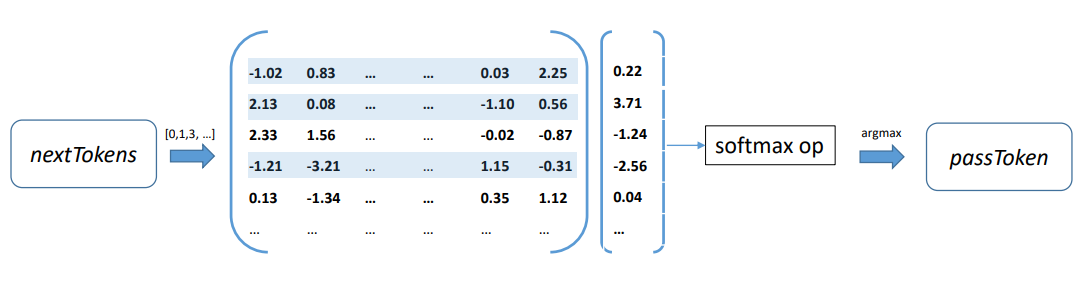
Figure 3: Integrating grammatical continuations into a log-linear model at one prediction step; rows selected by nextTokens are shadowed in blue.

4.2 Integrating Grammar into Neural Models

After calculating the permissible next tokens, we can restrict predictions in order to improve both prediction time and accuracy. We apply this general strategy to the prediction layer of our RNN-based neural network (a linear layer + softmax operation, which can be seen as a log-linear model Dymetman and Xiao (2016)), although it should be applicable to other prediction models, such as multi-class SVMs Duan and Keerthi (2005) or random forests Ho (1995).

Figure 3 illustrates a concrete example of integrating the grammar (represented as an automaton in our case) into the token prediction model at a particular prediction step. We focus on the prediction layer of the model, which consists of one linear layer followed by the softmax operation. The linear layer involves a matrix of size $\mbox{$|V|$}\times d$, where $V$ is the LF vocabulary and $d$ is the dimension of the vector passed from the previous layer; the linear layer predicts scores for each of the $V$ tokens before they are passed to softmax operation.

To integrate the grammar, first, the function nextTokens is called to return a list of tokens allowed by the grammar at this prediction step; the valid tokens are then translated into a list of indices, denoted by $l_{c}$, which is passed to the log-linear model. Supposing there are $k$ indices in the list $l_{c}$, we can dynamically construct another matrix of size $k\times d$ where the $i^{\mbox{\em th}}$ row in the new matrix corresponds to the $j^{\mbox{\em th}}$ row in the original matrix, for $j=l_{c}[i]$. Figure 3 illustrates this process of choosing rows from the original matrix to construct the new matrix.

Then the new matrix-vector product will result in scores only for those $k$ LF tokens that are permissible, and will then be passed to the softmax operation. The decision function (e.g., argmax in Figure 3) will then be applied based on the softmax score, whose results will finally be passed to passToken function to update the current DFA state.

Time Efficiency Concerns

We implement nextTokens to directly return a list of indices to avoid the cost of converting tokens to indices. We implemented our token prediction model in PyTorch, which supports slicing operations so that our on-the-fly matrix construction does not need to copy the original matrix data, but can instead just point to it. However, we find in our experiments that even matrix construction using slicing tends to be costly (see section 5).

To overcome this, we observe that we can enumerate the lists returned by nextTokens for every DFA state, and then cache the corresponding matrices. For example, consider RCM (the Relational Constraint Machine) in 2. We can cache the value of nextTokens for state 1 by precomputing the matrix corresponding to all the enum/num fields. Doing this caching for every DFA state can be expensive in memory; in practice, one may consider tradeoffs between memory consumption and prediction time.

5 Model and Experiments

5.1 EQS Dataset

Our experiments are conducted on the EQS dataset. The dataset consists of queries paired with their LFs, which were obtained in a semi-automated manner. The dataset contains 1981 (NL, LF) pairs as training data and 331 (NL, LF) pairs as test data. The LF vocabulary size is 56209, most of which consists of enum field names and values. All the LFs can be accepted by the FSA discussed in Section 3.

The dataset is too small to effectively learn a model that can reliably predict rare fields or values. However, as most of the queries involve only common fields and entities, we find in our experiments that our neural semantic parser is able to parse a large number of those queries correctly; orthogonal research is being conducted on how to handle more rare fields or entities.

5.2 Baseline Neural Model

We use a seq2seq neural architecture as our baseline. For our encoder, we initialize the word embeddings using Glove vectors Pennington et al. (2014); then a Bi-LSTM is run over the question where the last output is used to represent the meaning of the question. For the decoder, we again use an LSTM that runs over LF prefixes, where the LF token embeddings are learned during training. Our decoder is equipped with an attention mechanism Luong et al. (2015) used to attend over the output of the Bi-LSTM encoder. We use greedy decoding to predict the LFs.

We choose hyperparameters based on our previous experience with this dataset. The word and LF token embeddings have 150 dimensions. The Bi-LSTM encoder is of dimension 150 for its hidden vector in each direction, therefore the decoding LSTM is of dimension 300 for its hidden vector. We train the model with RMSprop Tieleman and Hinton (2012) for 50 epochs.

Our baseline neural model achieves 80.33% accuracy on the test set. Most of the errors made by our model are due to unseen fields or values; we observe that our model also fails on queries involving compositionality patterns that have not been seen in training, a problem similar to those reported by Lake and Baroni (2018).

5.3 Experimental Setups

All our experiments were conducted on a server with 40 Intel Xeon@3.00GHz CPUs and 380 GB of RAM. We monitor the server state closely while conducting the experiments.

Our models are implemented in PyTorch Paszke et al. (2017), which is able to exploit the server’s multi-core architecture. The peak usage for both CPU load and memory consumption for all our models is far below the server’s capacity.

We run all the models over the entire test dataset (331 sentences) and report the average prediction time for each sentence. For each model, we conduct 5 such runs to calculate the standard deviations of different runs. The standard deviations are small in absolute and relative value.

5.4 Results

Integrating the LF grammar into prediction at decoding time eliminates all grammatical errors and can therefore improve accuracy. This has been shown, for example, by Xiao et al. (2016); Yin and Neubig (2018), and indeed we obtain similar accuracy improvements. By incorporating the grammar at decoding time at all decoding steps (using its superset represented as an automaton), our parser is able to eliminate some grammatical errors, achieving 80.67% accuracy on the test set, which improves our baseline model by 0.30%.

Table 1 shows the main results of our experiments. Our baseline neural semantic parser (NSP) takes on average 0.260 seconds to predict the LF for a given query. When we use the model that integrates the LF grammar but constructs the reduced matrices on the fly (GSP-G), we find that despite the reduction of average permissible tokens (from 56209 to 6336), the prediction time actually increases drastically to 4.416 seconds.

To shed some light on this, we integrate the grammatically permissible next tokens only when their number is (a) less than 500 and (b) less than $10^{4}$. We observe that when the number of permissible next tokens is small, as in case (a), integrating the grammar can indeed reduce prediction time, indicating that the slowing is due to the dynamic matrix construction that uses the PyTorch slicing operation, as nextTokens and passToken are called at every prediction step in all cases.

To avoid this, we cache the reduced matrices (subsection 4.2, NSP-GC in Table 1) and observe that prediction time decreases in this case when more grammar integration is applied. The best prediction time (0.067 second per query) is achieved by NSP-GC when the grammar is used at every step. But similar speed-ups can be achieved when we are using cached matrices only for states with a small nextTokens set.

Model	Avg time	Avg tokens
NSP	0.260 $\pm 0.002$	$56209$
NSP-G($500$)	$0.079\pm 0.000$	$9643$
NSP-G($10^{4}$)	$0.252\pm 0.000$	$6981$
NSP-G(all)	$4.416\pm 0.029$	$\mathbf{6336}$
NSP-GC($500$)	$0.074\pm 0.000$	$9643$
NSP-GC($10^{4}$)	$0.069\pm 0.000$	$6981$
NSP-GC(all)	$\mathbf{0.067\pm 0.000}$	$\mathbf{6336}$

Table 1: Prediction time (in seconds) and number of permissible tokens per query on average, for our baseline neural semantic parser (NSP) and various models using grammar integration with caching (NSP-GC) or without (NSP-G).

6 Related Work

Speeding up neural models that have a softmax bottleneck is an ongoing research problem in NLP. In machine translation, some approaches tackle the problem by moving from the prediction of word-level units to sub-word units Sennrich et al. (2016) or characters Chung et al. (2016). This approach can reduce the dimensionality of the softmax significantly, at the price of increasing the number of output steps and thus requiring the model to learn more long-distance dependencies between its outputs. The technique could easily be combined with the one described here; the only adaptation required would be to change the grammar so that it uses smaller units to define its language. In a finite-state context, this would mean replacing transitions corresponding to a single LF token with a sequence of transitions that construct the token from characters. This creates potential for memory savings as well, if states in these expanded transitions can be shared in a trie structure.

Another approach for ameliorating a softmax bottleneck is the use of a hierarchical softmax Morin and Bengio (2005), which is based on organizing all possible output values into a hierarchy or tree of clusters. A token to be emitted is chosen by starting at the root cluster and then picking a child cluster until a leaf is reached. A token in this leaf cluster is then selected. Our approach could be combined with the hierarchical softmax method by creating a specific version of the cluster hierarchy to be associated with every state. We would filter all impossible tokens for a state from the leaf clusters and then prune away empty clusters in a bottom-up fashion to obtain a specific cluster.

While they have not been used in order to speed up predictions, grammars describing possible output structures have been combined with neural models in a number of recent papers on semantic parsing Yin and Neubig (2017, 2018); Krishnamurthy et al. (2017); Xiao et al. (2016, 2017). These papers use grammars to guide the training of the neural network model and to restrict the decisions the model can make at training and prediction time in order to obtain more accurate results with less data. Our approach is focused on speed improvements and does not require any changes to the underlying model or training protocols.

Like our approach, the one presented by L’Hostis et al. (2016) for machine translation tries to limit the decoding vocabulary. Their approach relies on limiting the tokens allowed during decoding to those that co-occurred frequently with the tokens in the input. Because this might rule out tokens that are needed to construct the correct output, this may decrease model performance. Our approach is guaranteed to never rule out correct outputs. For additional performance gains it should be possible to combine both approaches.

7 Future Work

We have used superset approximations based on finite-state automata instead of directly using the grammar of the LF language, which will usually be context-free. This choice is driven by the need for an efficient implementation of passToken and nextTokens, which could be expensive for longer sequences when using a general context-free grammar. However, for those context-free grammars that are LR Knuth (1965), recognition can be performed in linear time, and it is easy to see that both passToken and nextTokens can then be implemented with O(1) time complexity on average. Furthermore, the caching mechanism we have proposed for nextTokens in this work is applicable in the case of LR grammars. Therefore, it would be possible to implement the methods proposed here for any LR grammar, and such grammars cover most LF languages in practical use.

For most LF languages there will be restrictions on the logical types of expressions that can occur in certain positions. We can detect some of these restrictions in our finite-state automata, but in general a type system could capture well-formedness conditions that cannot be easily expressed with FSAs, or even in context-free grammars. It would be interesting to investigate how more expressive type checking can be integrated into our present framework in a more general setting.

8 Conclusion

We propose a method to improve the time efficiency of seq2seq models for semantic parsing using a large vocabulary. We show that one can leverage a finite-state approximation to the LF language in order to speed up neural parsing significantly. Given a context-free grammar for the LF language, our strategy is general and can be applied to any model that predicts the output in a sequential manner.

In the future we will explore alternatives to finite-state automata, which potentially characterize the relevant LF languages exactly while still allowing for efficient computation of admissible next tokens. We also plan to experiment with additional datasets.

References

- Bengio et al. (2003) Yoshua Bengio, Réjean Ducharme, Pascal Vincent, and Christian Janvin. 2003. A neural probabilistic language model. Journal of Machine Learning Research, 3:1137–1155.
- Chung et al. (2016) Junyoung Chung, Kyunghyun Cho, and Yoshua Bengio. 2016. A character-level decoder without explicit segmentation for neural machine translation. In Proceedings of the 54th Annual Meeting of the Association for Computational Linguistics, pages 1693–1703.
- Dahl et al. (1994) Deborah A. Dahl, Madeleine Bates, Michael Brown, William Fisher, Kate Hunicke-Smith, David Pallett, Christine Pao, Alexander Rudnicky, and Elizabeth Shriberg. 1994. Expanding the scope of the atis task: The atis-3 corpus. In Proceedings of the Workshop on Human Language Technology, pages 43–48.
- Dong and Lapata (2016) Li Dong and Mirella Lapata. 2016. Language to logical form with neural attention. In Proceedings of the 54th Annual Meeting of the Association for Computational Linguistics, pages 33–43.
- Dong and Lapata (2018) Li Dong and Mirella Lapata. 2018. Coarse-to-fine decoding for neural semantic parsing. In Proceedings of the 56th Annual Meeting of the Association for Computational Linguistics, pages 731–742.
- Duan and Keerthi (2005) Kai-Bo Duan and S. Sathiya Keerthi. 2005. Which is the best multiclass svm method? an empirical study. In Proceedings of the 6th International Conference on Multiple Classifier Systems, pages 278–285.
- Dymetman and Xiao (2016) Marc Dymetman and Chunyang Xiao. 2016. Log-linear rnns: Towards recurrent neural networks with flexible prior knowledge. CoRR, abs/1607.02467.
- Earley (1970) Jay Earley. 1970. An efficient context-free parsing algorithm. Communications of the ACM, 13(2):94–102.
- Ho (1995) Tin Kam Ho. 1995. Random decision forests. In Proceedings of the Third International Conference on Document Analysis and Recognition, pages 278–282.
- Knuth (1965) Donald E. Knuth. 1965. On the translation of languages from left to right. Information and Control, 8(6):607–639.
- Krishnamurthy et al. (2017) Jayant Krishnamurthy, Pradeep Dasigi, and Matt Gardner. 2017. Neural semantic parsing with type constraints for semi-structured tables. In Proceedings of the 2017 Conference on Empirical Methods in Natural Language Processing, pages 1516–1526.
- Lake and Baroni (2018) Brenden M. Lake and Marco Baroni. 2018. Generalization without systematicity: On the compositional skills of sequence-to-sequence recurrent networks. In Proceedings of the 35th International Conference on Machine Learning, pages 2879–2888.
- L’Hostis et al. (2016) Gurvan L’Hostis, David Grangier, and Michael Auli. 2016. Vocabulary selection strategies for neural machine translation. CoRR, abs/1610.00072.
- Liang et al. (2017) Chen Liang, Jonathan Berant, Quoc Le, Kenneth D. Forbus, and Ni Lao. 2017. Neural symbolic machines: Learning semantic parsers on freebase with weak supervision. In Proceedings of the 55th Annual Meeting of the Association for Computational Linguistics, pages 23–33.
- Luong et al. (2015) Thang Luong, Hieu Pham, and Christopher D. Manning. 2015. Effective approaches to attention-based neural machine translation. In Proceedings of the 2015 Conference on Empirical Methods in Natural Language Processing, pages 1412–1421.
- Mikolov et al. (2010) Tomas Mikolov, Martin Karafiát, Lukás Burget, Jan Cernocký, and Sanjeev Khudanpur. 2010. Recurrent neural network based language model. In Interspeech, pages 1045–1048.
- Morin and Bengio (2005) Frederic Morin and Yoshua Bengio. 2005. Hierarchical probabilistic neural network language model. In Proceedings of the Tenth International Workshop on Artificial Intelligence and Statistics, pages 246–252.
- Nederhof (2000) Mark-Jan Nederhof. 2000. Practical experiments with regular approximation of context-free languages. Computational Linguistics, 26(1):17–44.
- Paszke et al. (2017) Adam Paszke, Sam Gross, Soumith Chintala, Gregory Chanan, Edward Yang, Zachary DeVito, Zeming Lin, Alban Desmaison, Luca Antiga, and Adam Lerer. 2017. Automatic differentiation in pytorch. In NIPS 2017 Workshop Autodiff.
- Pennington et al. (2014) Jeffrey Pennington, Richard Socher, and Christopher Manning. 2014. Glove: Global vectors for word representation. In Proceedings of the 2014 Conference on Empirical Methods in Natural Language Processing, pages 1532–1543.
- Rabin and Scott (1959) M. O. Rabin and D. Scott. 1959. Finite automata and their decision problems. IBM Journal of Research and Development, 3(2):114–125.
- Sennrich et al. (2016) Rico Sennrich, Barry Haddow, and Alexandra Birch. 2016. Neural machine translation of rare words with subword units. In Proceedings of the 54th Annual Meeting of the Association for Computational Linguistics, pages 1715–1725.
- Tieleman and Hinton (2012) T. Tieleman and G. Hinton. 2012. Lecture 6.5—RmsProp: Divide the gradient by a running average of its recent magnitude. COURSERA: Neural Networks for Machine Learning.
- Xiao et al. (2016) Chunyang Xiao, Marc Dymetman, and Claire Gardent. 2016. Sequence-based structured prediction for semantic parsing. In Proceedings of the 54th Annual Meeting of the Association for Computational Linguistics, pages 1341–1350.
- Xiao et al. (2017) Chunyang Xiao, Marc Dymetman, and Claire Gardent. 2017. Symbolic priors for rnn-based semantic parsing. In Proceedings of the Twenty-Sixth International Joint Conference on Artificial Intelligence, IJCAI-17, pages 4186–4192.
- Yin and Neubig (2017) Pengcheng Yin and Graham Neubig. 2017. A syntactic neural model for general-purpose code generation. In Proceedings of the 55th Annual Meeting of the Association for Computational Linguistics, pages 440–450.
- Yin and Neubig (2018) Pengcheng Yin and Graham Neubig. 2018. Tranx: A transition-based neural abstract syntax parser for semantic parsing and code generation. In Proceedings of the 2018 Conference on Empirical Methods in Natural Language Processing: System Demonstrations, pages 7–12.
- Yu et al. (2018) Tao Yu, Michihiro Yasunaga, Kai Yang, Rui Zhang, Dongxu Wang, Zifan Li, and Dragomir R. Radev. 2018. Syntaxsqlnet: Syntax tree networks for complex and cross-domaintext-to-sql task. In Proceedings of the 2018 Conference on Empirical Methods in Natural Language Processing, pages 1653–1663.
- Zelle and Mooney (1996) John M. Zelle and Raymond J. Mooney. 1996. Learning to parse database queries using inductive logic programming. In Proceedings of the Thirteenth National Conference on Artificial Intelligence, AAAI 96, pages 1050–1055.