Cosmology of Lorentz fiber-bundle induced scalar-tensor theories
Abstract
We investigate the cosmological applications of scalar-tensor theories that arise effectively from the Lorentz fiber bundle of a Finsler-like geometry. We first show that the involved nonlinear connection induces a new scalar degree of freedom and eventually a scalar-tensor theory. Using both a holonomic and a non-holonomic basis, we show the appearance of an effective dark energy sector, which additionally acquires an explicit interaction with the matter sector, arising purely from the internal structure of the theory. Applying the theory at late times we find that we can obtain the thermal history of the universe, namely the sequence of matter and dark-energy epochs, and moreover the effective dark-energy equation-of-state parameter can be quintessence-like, phantom-like, or experience the phantom-divide crossing during cosmological evolution. Furthermore, applying the scenario at early times we see that one can acquire an exponential de Sitter solution, as well as obtain an inflationary realization with the desired scale-factor evolution. These features arise purely from the intrinsic geometrical structure of Finsler-like geometry, and reveal the capabilities of the construction.
pacs:
98.80.-k, 95.36.+x, 04.50.KdI Introduction
According to an increasing amount of data the universe experienced two phases of accelerating expansion, one at early and one at late cosmological times. Such a behavior may imply a form of extension of our current knowledge, in order to introduce the necessary extra degrees of freedom that would be needed for its successful explanation. In principle there are two main ways one could follow. The first is to assume that general relativity is correct however the matter content of the universe should be modified through the introduction of the inflaton Bartolo:2004if and/or dark energy fields Copeland:2006wr ; Cai:2009zp . The second way is to consider that the gravitational theory is not general relativity but a more fundamental theory, possessing the former as a particular limit, but which in general can provide the extra degrees of freedom needed for a successful cosmological description Capozziello:2011et ; Nojiri:2010wj ).
In order to construct gravitational modifications one starts from the Einstein-Hilbert Lagrangian of general relativity and includes extra terms, such as in gravity Starobinsky:1980te ; Capozziello:2002rd and Lovelock gravity Lovelock:1971yv ; Deruelle:1989fj , or even he can use torsion such as in gravity Cai:2015emx and in gravity Kofinas:2014owa . Alternatively, one may consider the general class of scalar-tensor theories, which include one extra scalar degree of freedom with general couplings with curvature terms. One general family of scalar-tensor theories is the Horndeski construction Horndeski:1974wa , re-discovered in the framework of generalized galileons Nicolis:2008in ; Deffayet:2009mn .
One interesting class of modified gravity theories may arise through the more radical modification of the underlying geometry itself, namely considering Finsler or Finsler-like geometries kour-stath-st 2012 ; Triantafyllopoulos:2018bli ; Minas:2019urp ; Basilakos:2013hua ; Basilakos:2013ij ; Kouretsis:2010vs ; Mavromatos:2010jt . These geometries extend in a natural way the Riemannian one, by allowing the physical quantities to have a dependence on the observer 4-velocity, which in turn reflects the Lorentz-violating character of the kinematics Bogoslovsky:1999pp ; Chang:2007vq ; Vacaru:2010fi ; Kostelecky:2008be ; Foster:2015yta ; Kostelecky:2011qz ; Kostelecky:2012ac ; Stavrinos:2012ty ; Hohmann:2016pyt ; Hohmann:2018rpp ; Pfeifer:2019wus . Furthermore, since Finsler and Finsler-like geometries are strongly related to the effective geometry within anisotropic media Born , entering naturally the analogue gravity approach Barcelo:2005fc , they may play an important role in quantum gravity considerations. In such a geometrical setup, the dependence of the metric and other quantities on both the position coordinates of the base-manifold as well as on the directional/velocity variables of the tangent space or scalar/spinor variables, makes the tangent bundle, or a fiber bundle of a smooth manifold, the natural geometrical framework for their description. Finally, the Riemannian case is reproduced from Finsler geometry if the velocity-dependence is set to zero.
If one applies the above into a cosmological framework he obtains Finsler and Finsler-like cosmologies. The basic feature of these is the appearance of extra terms in the Friedmann equations due to the intrinsic geometrical spacetime anisotropy of Finsler and Finsler-like geometries stavrinos-ikeda 1999 ; stavrinos-ikeda 2000 ; Stavrinos:2012ty ; kour-stath-st 2012 ; Stavrinos:2016xyg ; Triantafyllopoulos:2018bli ; Minas:2019urp (note that the term “spacetime anisotropy” in this framework is related to the Lorentz violation features of the geometry and should not be confused with the spatial anisotropy that can exist in Riemannian geometry too, e.g. in Bianchi cases). In specific subclasses of the theory, one can show that these novel features are quantified by effective degrees of freedom that behave as scalars under coordinate transformations. Hence, one can obtain an effective scalar-tensor theory arising from a Lorentz fiber bundle. The research of the Finslerian scalar-tensor theory of gravitation started in stavrinos-ikeda 1999 ; stavrinos-ikeda 2000 and later in Stavrinos:2016xyg , giving an extension of Riemannian ansatz of the scalar-tensor theory of gravitation. Additionally, since Finslerian theories exhibit in general a violation of Lorentz invariance, one may examine their relation with other classes of theories that have a preferred vector field or break Lorentz symmetry, such as Horava-Lifshitz gravity, Einstein-aether theories and field theories with Lorentz-violating matter fields Vacaru:2010rd ; Foster:2015yta ; Edwards:2018lsn .
In the present work we are interested in investigating the cosmological applications of the scalar-tensor theory that arises from a Lorentz fiber bundle. As we will see, the construction of a Lorentz fiber bundle can provide us an alternative approach of the cosmological dynamics of scalar-tensor gravitational theory. In this framework one obtains extra terms in the Friedmann equations that can lead to interesting cosmological results.
The plan of the work is the following: In Section II we present the geometrical background of our construction, namely referring to the Lorentz fiber bundle structure, the role of the connection and the geodesics. In Section III we introduce the actions of the theory and we show how a scalar-tensor theory can effectively appear from the structure of a fiber bundle. Then in Section IV we investigate in detail the cosmological applications of the constructed theories, both at late and early times. Finally, we summarize the obtained results in Section V.
II Geometrical Background
In this section we briefly review the basic features of Finsler geometry.
II.1 Basic structure of the Lorentz fiber bundle
Let us present the geometrical framework under consideration (a detailed investigation can be found in stavrinos-ikeda 1999 ; stavrinos-ikeda 2000 ). We consider a 6-dimensional Lorentz fiber bundle over a 4-dimensional pseudo-Riemannian spacetime manifold , which locally trivializes to the form . The local coordinates on this structure are with the coordinates on the base manifold, where take the values from to , and the coordinates on the fiber where take the values and . A coordinate transformation on the fiber bundle maps the old coordinates to the new as:
| (1) | ||||
| (2) |
where is the Kronecker symbol for the corresponding values, and the Jacobian matrix is non-degenerate.
Moreover, the space is equipped with a nonlinear connection with local components . The nonlinear connection plays a fundamental role in the theory of Lorentz tangent bundle and vector bundles Triantafyllopoulos:2018bli ; Minas:2019urp ; Stavrinos:2012ty . It is a geometrical structure that connects the external- (horizontal) spacetime with the internal- (vertical) space. This nonlinear connection induces a unique split of the total space into a horizontal distribution and a vertical distribution , with
| (3) |
The adapted basis to this split is
| (4) |
with and . The vectors span the horizontal distribution, while span the vertical distribution. Furthermore, the dual basis is
| (5) |
with a summation implied over the possible values of . Capital indices span all the range of values of indices on a fiber bundle’s tangent space. Finally, the basis vectors transform as:
| (6) |
| (7) |
where a summation is implied over the possible values of . From these we finally acquire the transformation of the nonlinear connection components as
| (8) |
II.2 Metric tensor and linear connection
The metric structure of the space is defined as
| (9) |
where has a Lorentzian signature . As we can see the fiber variables play the role of internal variables. The metric components for the fiber coordinates are set as and . The inverse metric components are defined by the relations and . Additionally, the transformation rules for the metric are calculated as
| (10) | |||
| (11) |
Note that the last relation implies that the metric components on the fiber are scalar functions of , since under a coordinate transformation we acquire and , or equivalently . Hence, as we mentioned in the Introduction, the internal structure of the Lorentz fiber bundle induces scalar degrees of freedom. This feature lies in the center of the analysis of this work.
One can define a linear connection in this space, where the following rules hold:
| (12) | ||||
| (13) |
Differentiation of the inner product and use of (12),(13) leads to the rules:
| (14) | ||||
| (15) |
It is apparent from the above relations that preserves the horizontal and vertical distributions, while maps one to the other.
Following the above rules, covariant differentiation of a vector along a horizontal direction gives:
| (16) |
where we have defined
| (17) | |||
| (18) |
Similarly, for the covariant differentiation of along a vertical direction we obtain
| (19) |
where we have defined
| (20) | |||
| (21) |
Finally, the covariant derivative for a tensor of general rank is obtained in a similar way.
The nonzero components for a metric-compatible connection , with , are uniquely calculated as:
| (22) | |||
| (23) | |||
| (24) | |||
| (25) |
with
| (26) |
while , etc. are Kronecker symbols.
Now, the curvature tensor of a linear connection is defined as the vector-valued map
| (27) |
where are vector fields on . Its local components in the adapted basis are defined as
| (28) |
where
| (29) |
with . The generalized Ricci tensor is then defined as
| (30) |
and the corresponding scalar curvature is . For the linear connection components (22)-(25) one obtains:
| (31) | |||
| (32) |
with the Ricci tensor of the Levi-Civita connection, and . Lastly, the scalar curvature is then
| (33) |
with .
From the above it becomes clear that the internal properties of the Lorentz fiber bundle eventually induce a scalar-tensor structure. This is the central feature of our work, and it will be later investigated in a cosmological framework.
II.3 Geodesics
A tangent vector to a curve is written as:
| (34) |
with and . Geodesics are the curves with an autoparallel tangent vector, namely
| (35) |
This relation leads to the following geodesic equations:
| (36) | |||
| (37) |
Relation (36) is identical with the geodesics equation of general relativity. The new equation of Finsler-like geometry is (37), which relates the fiber velocity with the velocity on spacetime via the nonlinear connection . From geodesic equations (36),(37) one can see that test particles obey the weak equivalence principle. However, Finsler and Finsler-like theories, similarly to general scalar-tensor theories, may violate the strong equivalence principle Puetzfeld:2015jha ; Alberte:2019llb ; Barausse:2017gip . Hence, in the end one should check whether these violations are inside the corresponding experimental bounds.
III Scalar tensor theories from the Lorentz fiber bundle
III.1 Field equations
Having presented the foundations and the underlying structure of this form of Finsler-like geometry, in this section we proceed by constructed physical theories. In particular, we can write an action as
| (38) |
where . Following Minas:2019urp we will consider two cases of Lagrangian densities:
-
1.
A Lagrangian density of the form
(39) where is a potential for the scalar , and
(40) is the curvature for the specific case of a holonomic basis , in order for the last term in (33) to vanish. Note that the presence of the scalar field in the denominators, that will be also transferred to the field equations below, requires to choose the potential in a suitable way in order for the dynamics not to lead to divergences. This is a requirement that holds for the prototype of scalar-tensor theories, namely the Brans-Dicke theory, as well as for large classes of Horndeski theories in which scalar-field-related terms appear in denominators.
-
2.
A Lagrangian density of the form
(41) on a non-holonomic basis, where the noninear connection components are considered as functions of , and .
Additionally, and in order to eventually investigate cosmological applications, we add the matter sector too, considering the total action
| (42) |
Since for the determinants and we have the relation , the above total action can be re-written as
| (43) |
Finally, the same relation holds for the second case, namely for the action of .
For the first case we insert the Lagrangian density (39) into the action (43) and we vary with respect to and . For we extract the equations:
| (44) |
where is the gravitational constant, is the Einstein tensor, and is the energy-momentum tensor. Additionally, the scalar-field equation of motion reads as
| (45) |
where a prime denotes differentiation with respect to .
For the second case we use the Lagrangian density (41), i.e. the full scalar curvature (33) without any potential for the scalar. Variation of the action (43) with respect to and gives the equations:
| (46) |
with
| (47) |
and
| (48) |
Hence, in order to proceed we need to consider a specific form of . We choose the following general form:
| (49) |
where is a real function of . Taking into account relations (47) and (49) we acquire the new form of the nonlinear connection components, namely . Thus, substitution into equations (46) and (48) gives:
| (50) |
and
| (51) |
where a prime denotes differentiation with respect to .
We close this subsection by discussing whether the constructed theory is free from pathologies. In general, in any theory first of all one needs to examine whether there are Ostrogradsky ghosts, namely whether the theory has higher-order (time) derivatives in the general equations of motion. Note that if the theory has second-order field equations then it is guaranteed that it does not have Ostrogradsky ghosts, however if it does have higher-order field equations it is not guaranteed that it does have Ostrogradsky ghosts, since the higher-order terms may correspond to extra degrees of freedom with second-order field equations (for instance this is the case of gravity as the Hamiltonian analysis reveals).
As one can see, for the first case of the Lagrangian density (39), namely in the equations of motion (44),(45), higher than second-order derivatives are absent. Similarly, for the second case of the Lagrangian density (41), namely in the equations of motion (46),(48), imposing the non-linear connection (49) (which does not include higher than first derivatives) leads to field equations (50),(51) where higher than second-order derivatives are absent. Hence, we deduce that our theory satisfies the basic requirement to be free from Ostrogradsky ghosts.
Nevertheless, it is well known that even if a theory is free from Ostrogradsky ghosts, still other kinds of pathologies, like ghost and Laplacian instabilities, may arise, related to the perturbation analysis, around a general or particular background(s). In order to examine whether the theory at hand exhibits such instabilities a full perturbation analysis is needed. However, the present work is devoted to a first study of the cosmological applications of the theory, and hence we focus on the basic requirement that the theory is free from Ostrogradsky ghosts. The full investigation of ghosts and Laplacian instabilities lies beyond the scope of the work and it is left for a future project.
III.2 Energy-momentum conservation
In this subsection we investigate the energy-momentum conservation in our model. A full analysis goes beyond the scope of this manuscript, however with some simple reasoning we can extract important results.
In Einstein’s general relativity, diffeomorphism invariance of the theory leads to energy-momentum conservation with respect to the Levi-Civita connection, through the Bianchi identities. In order to examine what happens in our case we may consider infinitesimal local diffeomorphisms on the Lorentz fiber-bundle induced by a vector field:
| (52) |
where the spacetime components of the vector are only dependent in order to be compatible with the transformation group of coordinates given in (1). Thus, a point with spacetime coordinates is mapped via the diffeomorphism to a point with spacetime coordinates , where is sufficiently small.
We consider the metric (9). Since depends only on and not on , mathematically it behaves like a pseudo-Riemannian metric of spacetime. The transformation rule for this kind of metric under a diffeomorphism is
| (53) |
where is the Levi-Civita connection and the parenthesis denotes symmetrization of indices. Additionally, the scalar field transforms as
| (54) |
In the following, we will assume that .
Now, it is known that the action
| (55) |
on a closed subspace of some dimensional differential manifold with local coordinates , , for a scalar function , is invariant under a local diffeomorphism that vanishes at the boundary . Hence, applying the above local diffeomorphism on the variation of the matter action part of (42), namely on , we obtain:
| (56) |
where we have used the definition of the matter energy-momentum tensor , and where is the determinant of the induced metric and a normal vector field at the boundary . Setting that at , the first term after the last equality in (56) vanishes. Additionally, since can be chosen arbitrarily, the last relation finally implies:
| (57) |
This expression denotes a departure from general relativity. Specifically, the nonminimal coupling of to the matter fields in the action (43) induces an interaction term in the above generalization of energy-momentum conservation. This interaction will have interesting implications in the cosmological application of the next section. Finally, we mention that for a constant scalar field this relation reduces to the standard conservation law of general relativity.
IV Cosmology
In the previous section we constructed the physical theories, namely the actions, on the framework of Finsler geometry, considering the cases of holonomic (Lagrangian (39)) and non-holonomic (Lagrangian (41)) basis separately, and we extracted the field equations. In order to apply them in a cosmological framework we consider a homogeneous and isotropic spacetime with the bundle metric
| (58) |
The first line of (58) is the standard spatially flat Friedmann-Robertson-Walker (FRW) metric, while the second line arises from the additional structure of the Lorentz fiber bundle. Moreover, we consider the energy-momentum tensor of the matter perfect fluid:
| (59) |
with the energy density, the pressure and the bulk 4-velocity of the fluid. As usual, the first line of (58) defines the comoving frame on this spacetime and is at rest with respect to it. Finally, note that relation (59) can be derived from a Lagrangian density , and thus we will use this when the matter Lagrangian appears in the field equations.
IV.1 First case: holonomic basis
For the spacetime (58), and with the perfect fluid (59), the field equations (44) and (45) of the holonomic case give:
| (60) | |||
| (61) |
| (62) |
where is the Hubble parameter and a dot denotes differentiation with respect to coordinate time . In the following we investigate these equations in late and early times separately.
IV.1.1 Late-time cosmology
Observing the forms of the Friedmann equations (60),(61), we deduce that we can write them in the usual form
| (63) | |||
| (64) |
defining the effective dark energy density and pressure respectively as
| (65) | |||
| (66) |
and thus the corresponding equation-of-state parameter will be
| (67) |
Hence, as we mentioned in the introduction, in the present scenario of holonomic basis, we obtain an effective dark energy sector that arises from the intrinsic properties of the Finsler-like geometry, and in particular from the scalar-tensor theory of the Lorentz fiber bundle.
Inserting the definitions of and into the scalar field equation of motion (62), and using the Friedmann equations (60),(61), we find that
| (68) | |||
| (69) |
Interestingly enough, we find that the scenario at hand induces an interaction between the matter and dark energy sector, again as a result of the intrinsic geometrical structure (this was already clear by the presence of in the right-hand-side of (62)), with the total energy density being conserved as expected from the conservation of the total energy-momentum tensor. Actually, equations (68),(69), derived in a specific framework, reflect the general expression (57). Hence, although the geometrical scalar-tensor terms that appear in the Friedmann equations (60),(61) may be obtained from other theories too, such as the Horndeski theory Horndeski:1974wa or the theory of generalized galileons Nicolis:2008in ; Deffayet:2009mn , the interaction term is something that does not fundamentally exist in these theories. In summary, the scenario at hand does not fall into the Horndeski class, and thus it is interesting to examine its cosmological implications.
We mention here that in literature of interacting cosmology, in general the interaction terms are imposed by hand, namely one breaks by hand the total conservation law into and , with the phenomenological descriptor of the interaction that is then chosen at will or under specific theoretical justifications Barrow:2006hia ; Amendola:2006dg ; Chen:2008ft ; Gavela:2009cy ; Chen:2011cy ; Yang:2014gza ; Faraoni:2014vra . However, in the present scenario of scalar-tensor theory from the fiber bundle with a holonomic basis, we see that such an interaction term, and in particular , arises naturally from the Finsler-like structure of the geometry (note that although interaction functions of the form have been shown to present instabilities at early times if the involved dark-energy sector has a constant equation-of-state parameter Valiviita:2008iv , in the case of general dark energy equation of state such instabilities are absent). Such a property opens new directions to look at the appearance of the interaction terms, especially under the light of its significance to alleviate the tension Yang:2018euj ; Pan:2019gop , and it is one of the main results of the present work.
Let us now investigate the cosmological behavior that is induced from the scenario at hand. We elaborate the Friedmann equations (60),(61) numerically, using as usual as independent variable the redshift , defined through (we set the present scale factor to ). We use various potential forms, such as linear, quadratic, quartic, and exponential. Moreover, we choose the initial conditions in order to obtain and in agreement with observations Ade:2015xua . Furthermore, for the matter sector we choose , namely the standard pressureless dust matter.
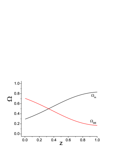
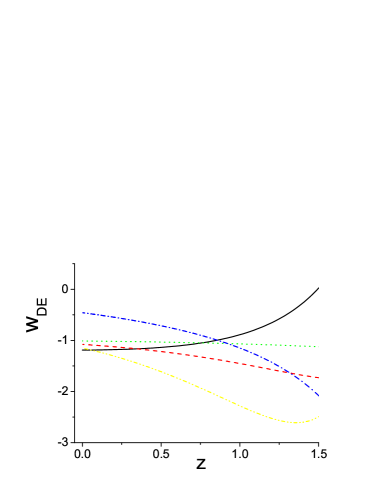
In Fig. 1 we present and for the case of quadratic potential , with . As we can see, we can obtain the usual thermal history of the universe, i.e. the sequence of matter and dark energy epochs, in agreement with observations, although we have not considered an explicit cosmological constant. Furthermore, in order to examine the effect of the potential forms on , in Fig. 2 we depict the evolution of for various potential choices, namely for linear , quadratic , quartic and exponential . We observe a rich behavior in the evolution of , which may lie in the quintessence or phantom regime, or experience the phantom-divide crossing. These properties are not easily obtained in theories with scalar degrees of freedom, and reveal the capabilities of the scenario.
IV.1.2 Inflation
We close this subsection by discussing the application of the scenario at hand in the case of early times, namely examining the inflationary realization. In this case the matter sector can be neglected. As one can easily see, the equations accept the de Sitter solution , which is the basis of any inflationary scenario. In particular, choosing the linear potential then (60),(61),(62) accept the solution
| (70) |
with an integration constant, if we choose . Note that the above de Sitter solution is obtained without considering an explicit cosmological constant.
Going into a more realistic inflationary realization, with a successful exit after a desired e-folding, and the desired scalar spectral index and tensor-to-scalar ratio, we can follow the method applied in Minas:2019urp and reconstruct the potential that produces any given form of . In particular, imposing the desired inflationary , Eq. (61) becomes a simple differential equation whose solution provides . Inserting this into (60) gives as
| (71) |
Note that in the absence of matter, Eq. (62) is not independent from (60),(61) and thus solution of the latter two ensures that (62) is satisfied too. Hence, knowing both and we can eliminate time and reconstruct explicitly the potential . Therefore, this potential is the one that generates the initially given inflationary . The capability of accepting inflationary solutions is an additional advantage of the scenario of Lorentz fiber-bundle induced scalar-tensor theory with holonomic basis.
We close this subsection by mentioning that in the above analysis we have indeed described the inflation epoch and the subsequent thermal history of the universe with the same model (relations (60)-(62)). However, we have used different potential and parameter choices for each case, which is standard in the literature since the involved energy scales in principle differ by many orders of magnitude. If one desires to construct a scenario that can describe the universe evolution from inflation to today in a unified way, he must introduce additional mechanisms/couplings that may successfully lead to quintessential inflation Hossain:2014zma ; Geng:2017mic . It would be interesting to see whether both pictures could be unified after an extension of the model with extra mechanisms.
IV.2 Second case: Nonholonomic basis
| (72) | |||
| (73) | |||
| (74) |
where a dot denotes a derivative with respect to and a prime denotes a derivative with respect to .
IV.2.1 Late-time cosmology
Similarly to the holonomic case of the previous subsection, we can re-write the Friedmann equations (72),(73) in the standard form (63),(64), introducing an effective dark energy sector with energy density and pressure respectively as
| (75) | |||
| (76) |
and thus the corresponding equation-of-state parameter is . Thus, in the present scenario of nonholonomic basis, we also obtain an effective dark energy sector that arises from the scalar-tensor theory of the Lorentz fiber bundle.
Inserting the above and into the scalar field equation of motion (74), and using the Friedmann equations (72),(73), we find that
| (77) | |||
| (78) |
Similarly to the holonomic case, in the present non-holonomic scenario the intrinsic geometrical structure induces an interaction between the matter and dark energy sector, while the total energy density is conserved. Therefore, the scenario at hand cannot be naturally obtained from Horndeski or generalized galileons theories.
We mention that although the above interaction term coincides with that of the holonomic case, namely , and despite the similarities of the Friedmann equations of the two cases, there is not a relation between of the holonomic case and of the non-holonomic case that could transform one case to the other. Hence, the two scenarios correspond to distinct classes of modified theories.
In order to investigate the cosmological evolution in this scenario one could perform a full numerical elaboration similar to the previous subsection, resulting to figures similar to Figs. 1 and 2. However, one can also extract approximate analytical solutions that hold at late times, namely in the dark energy epoch. In particular, as it is well known, a very general and important solution for the scale factor evolution is the power-law one, namely
| (79) |
in which case the Hubble function becomes
| (80) |
As an example we choose a linear form for , i.e. . In this case one can extract the approximate solutions of Eqs. (72),(73) and (74) as
| (81) | |||||
| (82) |
These lead to
| (83) | |||
| (84) |
and thus the asymptotic value of is
| (85) |
Hence, we can easily see that the universe at late times exhibits the correct thermal history, with the sequence of matter and dark energy epochs and the onset of late-time acceleration. Additionally, the dark-energy equation-of-state parameter may be quintessence-like, phantom-like, or experience the phantom-divide crossing during the evolution. Finally, acquires an asymptotic value which can lie in the quintessence regime, in the phantom regime, or being exactly equal to the cosmological constant value (by choosing ). We stress that the above behavior is obtained without considering an explicit cosmological constant, namely it arises solely form the fiber bundle structure of Finsler-like geometry, and this is an additional advantage that reveals the capabilities of the scenario.
Let us mention here that in the above example there appears a non-minimal coupling between the matter sector and the scalar field, and such couplings, may in general lead to violation of the equivalence principle. Hence, similarly to the theories where non-minimal matter couplings are used, such as in theories where the matter Lagrangian is coupled to Bertolami:2007gv , in gravity with the trace of the energy momentum tensor Harko:2011kv , etc, one should choose the involved model parameters in a way that the experimental bounds on the equivalence principle are satisfied.
IV.2.2 Inflation
We close this subsection by discussing the application of the scenario at hand in inflationary realization. Neglecting the matter sector, we focus on the existence of the de Sitter solution . Indeed, choosing then (72),(73),(74) accept the solution
| (86) |
with an integration constant, if we choose , or , , in units where . Similarly to the holonomic case, we mention that the above de Sitter solution is obtained without considering an explicit cosmological constant.
Finally, we close this analysis by describing the possibility to obtain any desired inflationary by suitably choosing the function . In particular, eliminating from (72),(73) gives the simple differential equation
| (87) |
which under the imposed provides the solution for . This can be substituted back in (72) and provide as
| (88) |
Thus, knowing both and we can reconstruct the form that produces the initially given inflationary .
We close the section by making the following comment. Strictly speaking, a more theoretically robust approach to the cosmological investigation would be to first construct a potential or a non-linear connection according to theoretical arguments, and then try to examine the induced dynamics. However, since the fundamental theory is unknown, in the analysis of the present section we followed the widely-used method of reconstructing the unknown functions of the theory in order to be consistent with the phenomenological requirements. The fact that the resulting forms for the potential and the non-linear connection may look complicated is not a problem, since this is known to be the case for all viable models of modified gravity (e.g. the viable and functions in the corresponding theories), under the requirement to incorporate phenomenology and observational data correctly.
V Conclusions
In the present work we investigated the cosmological applications of scalar-tensor theories that arise effectively from the Lorentz fiber bundle of a Finsler-like geometry. The latter is a natural extension of Riemannian one in the case where the physical quantities may depend on a set of internal variables, too. Hence, in a general application of such a construction to a cosmological framework, one obtains extra terms in the Friedmann equations that can lead to interesting phenomenology.
We started by a Lorentz fiber bundle structure, where represents a pseudo-Remannian spacetime with two fibers and . The nonlinear connection under consideration induces a new degree of freedom that behaves as a scalar under coordinate transformations. Hence, the rich structure of Finsler-like geometry can induce an effective scalar-tensor theory from the Lorentz fiber bundle.
In the case where a holonomic basis is used, the effective scalar-tensor theory leads to the appearance of an effective dark energy sector of geometrical origin in the Friedmann equations. However, the interesting novel feature is that we acquired an interaction between the matter and dark energy sectors, arising purely from the internal structure of the theory and not imposed by hand. Hence, the theory under consideration cannot be naturally obtained from Horndeski or generalized galileons theories. Applying it at late times we found that we can obtain the thermal history of the universe, namely the sequence of matter and dark-energy epochs, in agreement with observations. Additionally, we showed that the effective dark-energy equation-of-state parameter can be quintessence-like, phantom-like, or experience the phantom-divide crossing during cosmological evolution. These features were obtained although we had not considered an explicit cosmological constant, namely they arise purely from the intrinsic geometrical structure of Finsler-like geometry, which is a significant advantage. Finally, applying the scenario at early times we showed that one can acquire an exponential de Sitter solution, as well as obtain an inflationary realization with the desired scale-factor evolutions, and thus with the desired inflationary observables such as the spectral-index and the tensor-to-scalar ratio.
In the case of a non-holonomic basis we also obtained an effective dark energy sector, which moreover exhibits an explicit interaction with the matter sector. Concerning late times, we extracted approximate analytical solutions in which the scale factor has a power-law evolution. These solutions show the sequence of matter and dark energy epochs, in agreement with observations, and furthermore the corresponding dark-energy equation-of-state parameter can lie in the quintessence or phantom regime, or experience the phantom-divide crossing during the evolution, or even obtain asymptotically exactly the cosmological constant value. Finally, at early times the scenario at hand can also accept de Sitter solutions, as well as a successful inflationary realization with the desired spectral-index and the tensor-to-scalar ratio.
We would like to mention here that the fact that in the present scenario we obtain an interacting behavior, as well as a dark energy sector that can lie in the phantom regime, may be useful towards the solution of the tension, since as it has been investigated in the literature both features may successfully lead to its alleviation Yang:2018euj ; Pan:2019gop .
In summary, the rich structure of Finsler-like geometry can lead to interesting cosmological phenomenology at both early and late times. There are many interesting investigations that should be performed along these lines. One should use observational data from Type Ia Supernovae (SNIa), Baryon Acoustic Oscillations (BAO), Cosmic Microwave Background (CMB) shift parameter and temperature and polarization, direct Hubble constant observations, and data, in order to extract constraints on the involved forms and parameters. In particular, the confrontation with the CMB power spectrum might be quite interesting in light of the low- anomalies, since as we mentioned in the introduction Finsler geometry in general presents an intrinsic anisotropy (in the specific construction of the present work, which belongs to the more general class of Finsler-like geometries, the intrinsic anisotropy is replaced by the set of internal variables ). Nevertheless, such a full confrontation with observations lies beyond the scope of this work and it is left for future projects. Additionally, one could perform a detailed dynamical analysis in order to reveal the global behavior of the theory with Finsler-like cosmology, independently from the initial conditions. Finally, going beyond the cosmological framework, one could look for black hole solutions in these theories. These necessary studies are left for future investigations.
Acknowledgments
The authors would like to thank an anonymous referee for useful comments and suggestions. This research is co-financed by Greece and the European Union (European Social Fund-ESF) through the Operational Programme “Human Resources Development, Education and Lifelong Learning” in the context of the project “Strengthening Human Resources Research Potential via Doctorate Research” (MIS-5000432), implemented by the State Scholarships Foundation (IKY). This article is based upon work from COST Action “Cosmology and Astrophysics Network for Theoretical Advances and Training Actions”, supported by COST (European Cooperation in Science and Technology).
References
- (1) N. Bartolo, E. Komatsu, S. Matarrese and A. Riotto, Phys. Rept. 402, 103 (2004) [astro-ph/0406398].
- (2) E. J. Copeland, M. Sami and S. Tsujikawa, Int. J. Mod. Phys. D 15, 1753 (2006) [hep-th/0603057].
- (3) Y. F. Cai, E. N. Saridakis, M. R. Setare and J. Q. Xia, Phys. Rept. 493, 1 (2010) [arXiv:0909.2776 [hep-th]].
- (4) S. Capozziello and M. De Laurentis, Phys. Rept. 509, 167 (2011) [arXiv:1108.6266 [gr-qc]].
- (5) S. Nojiri and S. D. Odintsov, Phys. Rept. 505, 59 (2011) [arXiv:1011.0544 [gr-qc]].
- (6) A. A. Starobinsky, Phys. Lett. B 91, 99 (1980).
- (7) S. Capozziello, Int. J. Mod. Phys. D 11, 483 (2002) [gr-qc/0201033].
- (8) D. Lovelock, J. Math. Phys. 12, 498 (1971).
- (9) N. Deruelle and L. Farina-Busto, Phys. Rev. D 41, 3696 (1990).
- (10) Y. F. Cai, S. Capozziello, M. De Laurentis and E. N. Saridakis, Rept. Prog. Phys. 79, no. 10, 106901 (2016) [arXiv:1511.07586 [gr-qc]].
- (11) G. Kofinas and E. N. Saridakis, Phys. Rev. D 90, 084044 (2014) [arXiv:1404.2249 [gr-qc]].
- (12) G. W. Horndeski, Int. J. Theor. Phys. 10, 363 (1974).
- (13) A. Nicolis, R. Rattazzi and E. Trincherini, Phys. Rev. D 79, 064036 (2009) [arXiv:0811.2197 [hep-th]].
- (14) C. Deffayet, S. Deser and G. Esposito-Farese, Phys. Rev. D 80, 064015 (2009) [arXiv:0906.1967 [gr-qc]].
- (15) A. P. Kouretsis, M. Stathakopoulos and P. C. Stavrinos, Phys. Rev. D 82, 064035 (2010) [arXiv:1003.5640 [gr-qc]].
- (16) N. E. Mavromatos, S. Sarkar and A. Vergou, Phys. Lett. B 696, 300 (2011) [arXiv:1009.2880 [hep-th]].
- (17) S. Basilakos, A. P. Kouretsis, E. N. Saridakis and P. Stavrinos, Phys. Rev. D 88, 123510 (2013) [arXiv:1311.5915 [gr-qc]].
- (18) S. Basilakos and P. Stavrinos, Phys. Rev. D 87, no. 4, 043506 (2013) [arXiv:1301.4327 [gr-qc]].
- (19) A. P. Kouretsis, M. Stathakopoulos and P. C. Stavrinos, Phys. Rev. D 86, 124025 (2012) [arXiv:1208.1673 [gr-qc]].
- (20) A. Triantafyllopoulos and P. C. Stavrinos, Class. Quant. Grav. 35, no. 8, 085011 (2018).
- (21) G. Minas, E. N. Saridakis, P. C. Stavrinos and A. Triantafyllopoulos, Universe 5, 74 (2019) [arXiv:1902.06558 [gr-qc]].
- (22) P. C. Stavrinos and S. I. Vacaru, Class. Quant. Grav. 30, 055012 (2013) [arXiv:1206.3998 [astro-ph.CO]].
- (23) G. Y. Bogoslovsky and H. F. Goenner, Gen. Rel. Grav. 31, 1565 (1999) [gr-qc/9904081].
- (24) Z. Chang and X. Li, Phys. Lett. B 663, 103 (2008) [arXiv:0711.0056 [hep-th]].
- (25) S. I. Vacaru, Int. J. Mod. Phys. D 21, 1250072 (2012) [arXiv:1004.3007 [math-ph]].
- (26) V. A. Kostelecky and M. Mewes, Astrophys. J. 689, L1 (2008) [arXiv:0809.2846 [astro-ph]].
- (27) A. Kostelecky, Phys. Lett. B 701, 137 (2011) [arXiv:1104.5488 [hep-th]].
- (28) V. Alan Kostelecky, N. Russell and R. Tso, Phys. Lett. B 716, 470 (2012) [arXiv:1209.0750 [hep-th]].
- (29) J. Foster and R. Lehnert, Phys. Lett. B 746, 164 (2015) [arXiv:1504.07935 [physics.class-ph]].
- (30) M. Hohmann and C. Pfeifer, Phys. Rev. D 95, no. 10, 104021 (2017) [arXiv:1612.08187 [gr-qc]].
- (31) M. Hohmann, C. Pfeifer and N. Voicu, Phys. Rev. D 100, no. 6, 064035 (2019) [arXiv:1812.11161 [gr-qc]].
- (32) C. Pfeifer, arXiv:1903.10185 [gr-qc].
- (33) M. Born and E. Wolf, Cambridge University Press, England (1999).
- (34) C. Barcelo, S. Liberati and M. Visser, Living Rev. Rel. 8, 12 (2005) [Living Rev. Rel. 14, 3 (2011)] [gr-qc/0505065].
- (35) P.C. Stavrinos and S. Ikeda, Rep. Math. Phys. 44 221-230 (1999).
- (36) P.C. Stavrinos and S. Ikeda, Bulletin of Calcutta Mathematical Society 8 1-2 (2000).
- (37) P. C. Stavrinos and M. Alexiou, Int. J. Geom. Meth. Mod. Phys. 15, no. 03, 1850039 (2017) [arXiv:1612.04554 [gr-qc]].
- (38) S. I. Vacaru, Gen. Rel. Grav. 44, 1015 (2012) [arXiv:1010.5457 [math-ph]].
- (39) B. R. Edwards and V. A. Kostelecky, Phys. Lett. B 786, 319 (2018) [arXiv:1809.05535 [hep-th]].
- (40) D. Puetzfeld and Y. N. Obukhov, Phys. Rev. D 92, no. 8, 081502 (2015) [arXiv:1505.01285 [gr-qc]].
- (41) L. Alberte, Class. Quant. Grav. 36, no. 22, 225001 (2019) [arXiv:1901.07045 [hep-th]].
- (42) E. Barausse, PoS KMI 2017, 029 (2017) [arXiv:1703.05699 [gr-qc]].
- (43) J. D. Barrow and T. Clifton, Phys. Rev. D 73, 103520 (2006) [gr-qc/0604063].
- (44) L. Amendola, G. Camargo Campos and R. Rosenfeld, Phys. Rev. D 75, 083506 (2007) [astro-ph/0610806].
- (45) X. m. Chen, Y. g. Gong and E. N. Saridakis, JCAP 0904, 001 (2009) [arXiv:0812.1117 [gr-qc]].
- (46) M. B. Gavela, D. Hernandez, L. Lopez Honorez, O. Mena and S. Rigolin, JCAP 0907, 034 (2009) [arXiv:0901.1611 [astro-ph.CO]].
- (47) X. m. Chen, Y. Gong, E. N. Saridakis and Y. Gong, Int. J. Theor. Phys. 53, 469 (2014) [arXiv:1111.6743 [astro-ph.CO]].
- (48) W. Yang and L. Xu, Phys. Rev. D 89, no.8, 083517 (2014) [arXiv:1401.1286 [astro-ph.CO]].
- (49) V. Faraoni, J. B. Dent and E. N. Saridakis, Phys. Rev. D 90, no. 6, 063510 (2014) [arXiv:1405.7288 [gr-qc]].
- (50) J. Valiviita, E. Majerotto and R. Maartens, JCAP 0807, 020 (2008) [arXiv:0804.0232 [astro-ph]].
- (51) W. Yang, S. Pan, E. Di Valentino, R. C. Nunes, S. Vagnozzi and D. F. Mota, JCAP 1809, no. 09, 019 (2018) [arXiv:1805.08252 [astro-ph.CO]].
- (52) S. Pan, W. Yang, E. Di Valentino, E. N. Saridakis and S. Chakraborty, arXiv:1907.07540 [astro-ph.CO].
- (53) P. A. R. Ade et al. [Planck Collaboration], Astron. Astrophys. 594, A13 (2016) [arXiv:1502.01589 [astro-ph.CO]].
- (54) M. Wali Hossain, R. Myrzakulov, M. Sami and E. N. Saridakis, Int. J. Mod. Phys. D 24, no. 05, 1530014 (2015) [arXiv:1410.6100 [gr-qc]].
- (55) C. Q. Geng, C. C. Lee, M. Sami, E. N. Saridakis and A. A. Starobinsky, JCAP 1706, 011 (2017) [arXiv:1705.01329 [gr-qc]].
- (56) O. Bertolami, C. G. Boehmer, T. Harko and F. S. N. Lobo, Phys. Rev. D 75, 104016 (2007) [arXiv:0704.1733 [gr-qc]].
- (57) T. Harko, F. S. N. Lobo, S. Nojiri and S. D. Odintsov, Phys. Rev. D 84, 024020 (2011) [arXiv:1104.2669 [gr-qc]].