BSL: An R Package for Efficient Parameter Estimation for Simulation-Based Models via Bayesian Synthetic Likelihood
Abstract
Bayesian synthetic likelihood (BSL) (Price et al., , 2018) is a popular method for estimating the parameter posterior distribution for complex statistical models and stochastic processes that possess a computationally intractable likelihood function. Instead of evaluating the likelihood, BSL approximates the likelihood of a judiciously chosen summary statistic of the data via model simulation and density estimation. Compared to alternative methods such as approximate Bayesian computation (ABC), BSL requires little tuning and requires less model simulations than ABC when the chosen summary statistic is high-dimensional. The original synthetic likelihood relies on a multivariate normal approximation of the intractable likelihood, where the mean and covariance are estimated by simulation. An extension of BSL considers replacing the sample covariance with a penalised covariance estimator to reduce the number of required model simulations. Further, a semi-parametric approach has been developed to relax the normality assumption. In this paper, we present an R package called BSL that amalgamates the aforementioned methods and more into a single, easy-to-use and coherent piece of software. The R package also includes several examples to illustrate how to use the package and demonstrate the utility of the methods.
Keywords: approximate Bayesian computation, covariance matrix estimation, Markov chain Monte Carlo, likelihood-free methods, pseudo-marginal MCMC
1 Introduction
In the Bayesian framework, inference on the parameter of a statistical model is carried out using the posterior distribution , where is the observed data. Bayes’ theorem shows that by observing through the likelihood function , the prior knowledge can be updated to provide the posterior distribution,
In most applications, the evidence involves high dimensional integration and is intractable. Recovery of the posterior distribution often relies on sampling methods, such as Markov chain Monte Carlo (MCMC) and sequential Monte Carlo (SMC) (Del Moral et al., , 2006).
However, in complex models, the likelihood function can be intractable or very expensive to evaluate. The terminology “likelihood-free inference” typically refers to inference techniques that do not require direct evaluation of the likelihood function, but rely on model simulations to approximate the likelihood in some way. One successful method is approximate Bayesian computation (ABC) (Sisson et al., , 2018). ABC essentially estimates the intractable likelihood non-parametrically at with a simulation . The raw dataset is usually reduced down to summaries with a carefully chosen summary statistic function , where and are the dimension of the raw data and summary statistics, respectively. Denote the observed and simulated summary statistics as and , respectively. The ABC likelihood function is given by
where is a discrepancy function, which measures the distance between the observed and simulated summary statistics under a certain metric, e.g. the Euclidean distance. is a kernel weighting function, usually an indicator function for convenience, which links distance and tolerance . Here is used to trade-off between the bias and variance of the likelihood estimator, i.e. as approaches zero the bias reduces but the variance increases. In sampling methods like MCMC, a likelihood estimator with large variance can cause the Markov chain to get stuck and reduce efficiency (Doucet et al., , 2015).
Due to the non-parametric nature of the ABC likelihood estimate, ABC can be very inefficient when the summary statistic is high dimensional (Blum and François, , 2010), which is often referred to as the curse of dimensionality. Wood, (2010) proposes to use a multivariate normal distribution to approximate the likelihood function. Such an approximation is called the synthetic likelihood (SL). We later extend the term to not only the multivariate normal distribution but also other reasonable parametric approximations of the likelihood (Drovandi et al., (2015) provide a general framework for such methods). Price et al., (2018) analyse SL in the Bayesian framework and name it Bayesian synthetic likelihood (BSL). MCMC is used to explore the parameter space. The paper uses extensive empirical results to show that BSL can outperform ABC even when the model summary statistics show small departures from normality. BSL not only scales better with the summary statistic dimension, but also requires less tuning and can be accelerated with parallel computing. Recently, asymptotic properties of BSL have been derived under various assumptions. Frazier and Drovandi, (2019) develop a result for posterior concentration and Nott et al., (2019) show that the BSL posterior mean is consistent and asymptotically normally distributed.
In the standard BSL approach, the most obvious computational drawback is the need to generate a large number of simulations for estimating a high-dimensional covariance matrix in the SL. Several strategies have been devised to reduce the number of simulations for estimating the synthetic likelihood. An et al., (2019) propose to use the graphical lasso to estimate a penalised covariance and provide an algorithm for selecting the penalty to ensure reasonable mixing when placed inside an MCMC algorithm. Ong et al., 2018a consider the shrinkage estimator of Warton, (2008) in the context of variational Bayes synthetic likelihood to reduce the number of simualtions. Everitt, (2017) considers a bootstrap approximation to lower the variance of the SL estimator. Furthermore, the normality assumption of SL has also been put under inspection by An et al., (2018), which considers a more flexible approximation of the synthetic likelihood using a semi-parametric estimator with a Gaussian copula.
There are existing packages in R for likelihood-free inference. For example, the R packages abc (Csillery et al., , 2012) and EasyABC (Jabot et al., , 2013) exist for various ABC methods. The R package synlik (Fasiolo and Wood, , 2014) implements the classic SL method of Wood, (2010). The package provides diagonostic tools for the normal synthetic likelihood and incorporates MCMC to find the approximate posterior distribution. However, synlik is limited to only the standard SL approach. Outside of R, the ABCpy (Dutta et al., , 2017) package in Python includes most of the popular ABC algorithms and the standard SL approach.
Given the wide applicability of BSL (e.g. Karabatsos, , 2018; Barbu et al., , 2018), it is important that BSL methods are directly accessible to practitioners. In this paper we introduce our BSL R package, which implements the Bayesian version of synthetic likelihood and many of the extensions listed earlier together with additional functionality detailed later in the paper. The package is flexible in terms of the prior specification, the implementation of the model simulation function and the choice of the summary statistic function. Further, it includes several built-in examples to help the user learn how to use the package.
The rest of this paper is structured as follows. Section 2 provides a brief descriptions of the statistical background for SL and two shrinkage approaches that are implemented in our package. In Section 3, we introduce the main functionalities in BSL with an illustrative example. Section 4 concludes the paper with a summary and further discussion.
2 Bayesian Synthetic Likelihood
Following the notation in Section 1, we focus on reviewing three SL estimators to and two shrinkage covariance estimation methods in Section 2.1 to 2.4. Then we briefly introduce other implementation details in Section 2.5.
The SL estimator can be viewed as an auxiliary likelihood function where the subscript “A” denotes that we are using a parametric density approximation and is the parameter of this parametric family of densities. To link this auxiliary likelihood to the actual likelihood, there is actually a functional relationship between and , which may be denoted as . However, we drop the dependence on for notational convenience. The SL posterior is given by
Unfortunately, the mapping from to is typically unknown. However can be estimated with simulations. The estimated synthetic likelihood is placed within an MCMC algorithm to sample from the corresponding approximate posterior of . Below we describe the synthetic likelihood estimators supported by our package, which amount to choosing the form of and the type of estimator of .
2.1 Standard BSL Likelihood Estimator
Assume we have obtained a collection of simulations from the model at a proposed parameter value of , i.e. . The corresponding summary statistics are denoted as for . Following Wood, (2010), the SL is assumed to be roughly multivariate normal. The classic SL estimator can be written as
| (1) |
where is estimated with sample mean and covariance
| (2) | ||||
Although is an unbiased estimator of , is not an unbiased estimator of . However, empirical results demonstrate that the approximate posterior exhibits very weak dependence on (Price et al., , 2018). Nevertheless, if is prohibitively small, then there can be significant Monte Carlo error in the MCMC approximation of the BSL target.
2.2 Unbiased BSL Likelihood Estimator
Ghurye and Olkin, (1969) provide an unbiased estimator for the multivariate normal density based on independent simulations from it. Price et al., (2018) show the viability of this estimator by using it in place of the standard SL estimator within an MCMC algorithm. The estimator, denoted as uBSL, requires for unbiasedness to hold. The estimated auxiliary parameter can be written as , where . Definitions of and can be found in equation (2). The unbiased likelihood estimator is given by
| (3) | ||||
where
and
In spite of the fact that the normality assumption is rarely true in practice, the approximate posterior distributions obtained by uBSL show less dependence on when compared to BSL (Price et al., , 2018).
2.3 A Semi-Parametric BSL Likelihood Estimator
Although the estimators of equations (1) and (3) are straightforward to compute, the normality assumption of the summary statistic could be restrictive in some cases. It is thus of interest to consider a more robust likelihood estimator that can handle non-normal summary statistics whilst not sacrificing much on computational efficiency.
Here we briefly describe the semi-parametric likelihood estimator of An et al., (2018), which is aliased as “semiBSL” by the authors. The paper shows examples where BSL fails to produce accurate posterior approximations and provides additional robustness to non-normality of the summary statistics. The semiBSL estimator harnesses kernel density estimation (KDE) to non-parametrically estimate the univariate distributions of the summary statistics and uses the Gaussian copula to model the dependence amongst summaries. This semi-parametric estimator provides additional robustness over the multivariate normal assumption and is quick to apply.
The estimator involves two aspects; modelling the marginals and modelling the dependence structure. We first describe the non-parametric aspect of KDE. Denoting the marginals of as for , if the summary statistic is continuous or approximately continuous (e.g. large counts), a KDE of the -th marginal density is given by
| (4) |
where is a non-negative kernel function with bandwidth parameter . See Izenman, (1991) for a review and discussion about KDE. Similarly, the corresponding estimated cumulative distribution function can be obtained. The choice of the kernel function could be various. An et al., (2018) select the Gaussian kernel for simplicity and for its unbounded support.
By using KDE, the semiBSL estimator can accommodate non-normal marginal summary statistics. For the second aspect, semiBSL uses a Gaussian copula to model dependence between summaries. The density function for the Gaussian copula is given by
where is the correlation matrix, , is the inverse CDF of a standard normal distribution, and is a -dimensional identity matrix. The main appeal of the Gaussian copula here is that it is fast to estimate the correlation matrix (see details later). Combining the advantages from both aspects, we are then able to have a tractable likelihood estimator written as , where is estimated by , where and is given by equation (4). The full semiBSL density estimator is given by
| (5) |
Finally we provide details on obtaining . With a collection of simulations , it can either be estimated with maximum likelihood estimation, or as An et al., (2018) advocate, one could use the Gaussian rank correlation (GRC, Boudt et al., (2012)). The GRC estimator is known to be more robust. The -th entry of the GRC matrix is given by
where , and , is the rank function. Note that here the GRC is used to estimated the correlation matrix in semiBSL. However, our package also permits the use of the GRC in standard BSL to provide more robustness. In doing so, a transformation to the covariance matrix is needed afterwards.
We point out that when the data generation process is complicated, most of the computational cost will be spent on model simulations. Thus the computational overhead introduced by the semi-parametric likelihood estimator may be negligible relative to the standard SL estimator.
2.4 An Accelerated Likelihood Estimator with Shrinkage Estimation
We can see from equations (1) and (5) that both estimators involve estimation of a covariance or correlation matrix. The number of free parameters in the covariance matrix grows quadratically with the number of summary statistics. Thus, for a high-dimensional summary statistic, a large number of simulations may be required to estimate the likelihood with reasonable precision.
Here we introduce two shrinkage estimators of the covariance matrix that have shown to be useful in empirical examinations (An et al., , 2019; Ong et al., 2018a, ; An et al., , 2018). The shrinkage estimators can be applied to BSL and semiBSL. Note that we skip uBSL because the unbiasedness property will be violated with shrinkage estimation. The selection of the penalty parameter will be discussed later in Section 2.5. For clarification, we change the notations in this subsection temporarily and restore them back after. Let be samples from a multivariate normal distribution . The dimension of each sample is . is the sample covariance and is the precision matrix.
2.4.1 Graphical Lasso
The graphical lasso (Friedman et al., , 2008) aims to find a sparse precision matrix by maximising the following regularised log-likelihood
where is a constant, is the norm, and is the penalty parameter. The problem is solved with convex optimisation. The penalty parameter controls the sparsity in , where large leads to high sparsity and vice versa. We refer the readers to Friedman et al., (2008) for more details about the graphical lasso. In our package we use the graphical lasso implementation in the R package glasso (Friedman et al., , 2018).
2.4.2 Warton’s Estimator
Warton, (2008) introduces a straightforward shrinkage estimator that is extremely fast to compute but still performs well. Define as the diagonal matrix of , then the sample correlation matrix can be computed with . The Warton’s shrinkage for the correlation matrix is given by
where is the shrinkage parameter, is the identity matrix. The correlation matrix degenerates to the identity matrix as approaches . With a correlation to covariance conversion, we get the Warton’s covariance estimator for
2.5 Other Implementation Details
2.5.1 Incorporating BSL with MCMC
Once we have selected a likelihood function estimator, we can use a Bayesian sampling algorithm to sample from the BSL approximation to the posterior . This is currently achieved using MCMC in our package. Pseudo-code for the MCMC BSL algorithm is provided in Algorithm 1.
The number of simulations affects the variance of the likelihood estimator, which is very important in an MCMC algorithm. We want to be large enough so that the MCMC chain is very unlikely to get stuck at an overestimated likelihood value, but not so large that the computational efficiency is hindered. The value of can be loosely chosen depending on the number of free parameters in the likelihood function and adjusted based on the acceptance rate and MCMC effective sample size (ESS). Empirical evidence (Price et al., , 2018; An et al., , 2018) has shown that the approximate posterior distribution (BSL, uBSL and semiBSL) is remarkably insensitive to , provided that is not too small in which case the Monte Carlo error of the MCMC approximation can be large. Price et al., (2018) demonstrate empirically that aiming for a standard deviation of the synthetic log-likelihood estimator of around at a representative parameter value provides the most computational efficient results for standard BSL.
We recommended that the initial value of the Markov chain have non-negligible support under the BSL posterior. Our experience with MCMC BSL is that if the chain is initialised far in the tails of the BSL posterior, then MCMC BSL exhibits slow convergence. The initial value for the Markov chain may be sourced from experts, previous analyses in the literature or a short run of another likelihood-free algorithm.
2.5.2 Penalty Selection
An et al., (2019) introduce a penalty selection approach for BSLasso (BSL with graphical lasso). Our goal is to reduce the value of required while still maintaining a similar level of noise in the SL approximation. Denote as the standard deviation of the penalised log-likelihood estimator that we are aiming for. The value of is typically around , as suggested earlier. The algorithm for selecting the penalty parameter is given in Algorithm 2. Here we use for the penalty parameter for both the graphical lasso and Warton’s estimator for notational convenience.
3 Using the BSL Package
Two main functionalities that are offered in the BSL package are (1) running an MCMC algorithm with a chosen SL estimator to sample from the approximate posterior distribution, (2) selecting the penalty parameter with the given SL estimator and shrinkage method. Parallel computing is supported with the R package foreach (Microsoft Corporation and Weston, , 2017) so that the independent model simulations can be run on a multi-core computer. In this section, we use the built-in example ma2 to show the usage of functions.
3.1 Description of the MA(2) Example
Here we consider the MA(2), moving average of order , time series model with parameter . The parameter space is constrained to so that the process is stationary and invertible. The model has two favorable properties as an illustrative example, (1) the likelihood is tractable and hence sampling from the true posterior is feasible for comparisons, (2) the data generation process is fast. The model can be described with the following equation
where for is white noise. The prior is set to be uniform on the feasible region of the parameter space, and zero elsewhere. We set and use the raw data as the summary statistic. Note that the likelihood function is exactly multivariate normal with mean zero, , , and all other covariances are . We load the observed data and simulation function with
R> data("ma2", package = "BSL")
3.2 The Model Object
We first introduce the S4 class BSLModel that encloses all ingredients for our model; namely a simulation function (fnSim), a summary statistic function (fnSum), a point estimate or initial value of the parameter (theta0) and other optional arguments for the model we want to run (for example simArgs and fnLogPrior as given below). The first three must be provided to generate a valid BSLModel object. This is done by running the creator function BSLModel. For example, we run the following command for the MA(2) model
R> model <- BSLModel(fnSim = ma2_sim, fnSum = function(x) x,+ simArgs = list(T = 50), theta0 = c(0.6, 0.2),+ fnLogPrior = ma2_logPrior)
*** initialize "BSLMODEL" ***has simulation function: TRUEhas summary statistics function: TRUEhas initial guess / point estimate of the parameter: TRUErunning a short simulation test ...*** end initialize ***
We can see in the console message that upon initialisation, the BSLModel creator function automatically checks if the three requisites exist, and if one or more elements are missing the function will only create an empty object. By default the creator function also checks if the functions can run properly by running simulations as a short test. If the test takes too long or is undesired, it can be turned off with the flag test = FALSE. theta0 is the initial guess of the parameter value, and will be used as the starting value in MCMC. Next we discuss how to properly code the simulation, summary statistic and prior function. The model object is mostly created for internal usage, so the related S4 methods are not described here.
3.2.1 The Simulation Function
A fast simulation function is helpful for the simulation-based methods in this paper. The simulation function is coded by the user and must have the model parameter as its first argument. Other necessary arguments can be put after if needed. The output can be of any valid R class and will be sent to the corresponding summary statistic function as the input data directly.
For example, the built-in simulation function of the MA(2) example is a valid simulation function. The length of the time series is determined by the second argument , which can be set to a fixed value with simArgs = list(T = 50). simArgs must be a list of the additional arguments to be put into the simulation function fnsim.
R> ma2_sim
function (theta, T){ rand <- rnorm(T + 2) y <- rand[3:(T + 2)] + theta[1] * rand[2:(T + 1)] + theta[2] * rand[1:T] return(y)}<bytecode: 0x0000000004864c90><environment: namespace:BSL>
For most complex likelihood-free applications, the simulation process will not be as straightforward as the MA(2) example. If the model simulation is complex and time-consuming, we encourage users to write their own simulation function in C/C++ and use Rcpp (Eddelbuettel and Francois, , 2011) to call the function within R, as the running time of the algorithm is typically dominated by model simulations. For a reference text on writing functions in Rcpp, see Eddelbuettel, (2013). The ma2_sim function generates a single model realisation. If it is fast to produce more than one independent model simulation, for example if code vectorisation can be implemented, the BSL package also allows users to write the simulation function that directly simulates independent model simulations simultaneously. The code below shows how can this can be implemented for the MA(2) simulation function.
R> ma2_simVec = function(n, theta, T) {+ rand <- matrix(rnorm(n * (T + 2)), n, T + 2)+ y <- rand[, 3 : (T + 2)] + theta[1] * rand[, 2 : (T + 1)]+ + theta[2] * rand[, 1 : T]+ sapply(1 : n, function(i) list(y[i, ]))+ }
The vectorised simulation function can be loaded with argument fnSimVec; if it is loaded the vectorised simulation function will be used regardless of whether fnSim is provided or not. The input of fnSimVec must follow the order of , and additional arguments. Note that vectorised simulation is incompatible with parallel computing described later.
3.2.2 The Summary Statistic Function
For simplicity, we load the identity function that returns the same data as the summary statistic in the MA(2) example. Similar to fnSim, fnSum also takes additional arguments if desired. The additional arguments for the summary statistic function need to be put right after the data. These arguments can be saved as a list to sumArgs. The return argument of the summary statistic function must be a -dimensional vector of summary statistics.
3.2.3 The Log Prior Function
fnLogPrior computes the log density of the prior distribution. If the prior function is not provided, an improper flat prior will be used by default. However, in practice, defining a proper prior distribution is always recommended. This function should only take as its input argument, and the output must not be positive infinity. Note that the normalisation constant of the prior distribution can be ignored, as we do below for the MA(2) example.
R> ma2_logPrior
function (theta){ log(theta[2] < 1 & sum(theta) > -1 & diff(theta) > -1)}<bytecode: 0x000000000485bd68><environment: namespace:BSL>
3.3 The Main Function
The primary function of the package is bsl, which uses MCMC to draw samples from an approximation to the idealised BSL posterior distribution . The type of likelihood estimator described in Section 2 (BSL, uBSL and semiBSL) can be specified by the argument method. Shrinkage estimation on the covariance matrix in BSL and the correlation matrix in semiBSL can be specified with shrinkage. The minimal requirements of the bsl function include the observed data (y), the number of simulations for synthetic likelihood estimation (n), total number of MCMC iterations (M) and the covariance matrix of the normal random walk Metropolis algorithm (covRandWalk). For the MA(2) example, a minimalistic call to the main function that runs MCMC BSL (using the estimator of equation (1)) is given by the following command.
R> resultMa2BSL <- bsl(y = ma2$data, n = 500, M = 300000, model = model,+ covRandWalk = ma2$cov, method = ’BSL’, verbose = TRUE)
Similarly, we can run MCMC uBSL and semiBSL by changing the method option,
R> resultMa2uBSL <- bsl(y = ma2$data, n = 500, M = 300000, model = model,+ covRandWalk=ma2$cov, method = ’uBSL’, verbose = TRUE)
R> resultMa2SemiBSL <- bsl(y = ma2$data, n = 500, M = 300000, model = model,+ covRandWalk=ma2$cov, method = ’semiBSL’, verbose = TRUE)
The normal random walk covariance matrix, covRandWalk, should be defined based on the parameterisation used in the MCMC sampling; if a parameter transformation is employed, the covariance matrix should be specified accordingly.
3.3.1 Shrinkage of the Likelihood Estimator
Implementation of shrinkage methods described in Section 2.4 can be specified with arguments shrinkage ("glasso" for the graphical lasso estimator and "Warton" for Warton’s estimator) and penalty for the penalty value ( in the graphical lasso and in Warton’s estimator). Note that the shrinkage takes place on the covariance matrix for method BSL, and on the correlation matrix (of the Gaussian copula) for method semiBSL.
Shrinkage should only be used when there is a relatively large number of entries near zero in the precision matrix for graphical lasso and covariance matrix for Warton’s approach. This can be checked by inspecting the inverse correlation matrix or the correlation matrix at a representative parameter value. In the MA(2) example, we are able to calculate the true covariance matrix. For more complex models the covariance matrix can be estimated with a large number of model simulations at a reasonable parameter value. Here we use the ggcorrplot function in ggcorrplot (Kassambara, , 2019) to visualise the matrices. The visualisation of the correlation matrix and inverse correlation matrix for the MA(2) example are shown in Figure 1.
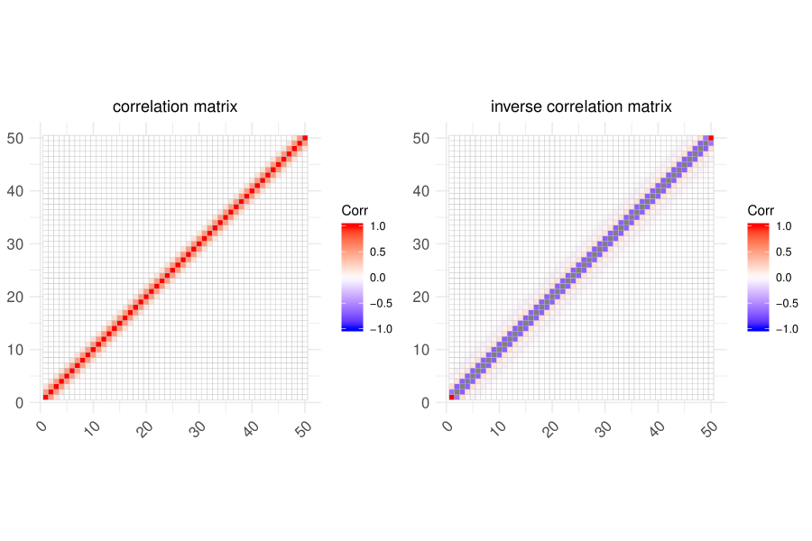
Both of the figures suggest that the correlation and inverse correlation matrices are sparse. It is also recommended to check the level of sparsity by computing the proportion of partial correlations below a certain threshold. For example, of the partial correlations between the summary statistics of the MA(2) example are below . Thus, for this example, shrinkage estimation is expected to reduce the number of model simulations required for estimating the synthetic likelihood whilst not sacrificing much on posterior accuracy. We will describe how to select the penalty parameter in our BSL package in Section 3.5. The following code runs MCMC BSL with the graphical lasso and Warton’s shrinkage estimator.
R> resultMa2BSLasso <- bsl(y = ma2$data, n = 300, M = 300000, model = model,+ covRandWalk=ma2$cov, method = ’BSL’, shrinkage = ’glasso’,+ penalty = 0.027, verbose = TRUE)R> resultMa2BSLWarton <- bsl(y = ma2$data, n = 300, M = 300000, model = model,+ covRandWalk=ma2$cov, method = ’BSL’, shrinkage = ’Warton’,+ penalty = 0.75, verbose = TRUE)
3.3.2 Parameter Transformation
If the prior distribution is bounded or the normal random walk cannot explore the parameter space efficiently, parameter transformation is recommended. Recall is the prior distribution for . Suppose the parameters are independent and bounded, the prior function can be decomposed as
where and are the lower and upper bound for . A straightforward but fruitful transformation that maps the range of the parameter to the real line is the logit transformation, which is given by
If the parameter is only bounded on one side, the transformation degenerates to a log transformation, i.e. if is and if is . The bsl function provides an easy-to-use log/logit transformation for independent and bounded parameters. The argument logitTransformBound is a by matrix containing the lower and upper bounds for each parameter. The only argument that needs to be changed is covRandWalk. There is no need to do any reparameterisation of the prior or simulation functions.
It is also possible to code a customised parameter transformation by editing the simulation function directly. If so the prior function should also be changed subject to the reparameterisation.
3.3.3 Parallel Computation
As a simulation-based method, the computational cost of BSL is mostly driven by the speed of the simulation process. Parallel computation is vital in complex applications where vectorisation is not possible. In our BSL package, the independent model simulations can be distributed across workers on a multi-core machine. The R package doParallel (Microsoft Corporation and Weston, , 2018) provides a way to set up the cpu cores for parallel computation. For example, the following code determines all the available cores of a cpu and sets up the clusters for parallel jobs.
R> ncores <- detectCores()R> cl <- makeCluster(detectCores())R> registerDoParallel(cl)
This should be turned on prior to running the main bsl function if parallel computing is desired. To enable parallel computing with in BSL, set parallel to TRUE in the bsl function. We utilise the function foreach of package foreach (Microsoft Corporation and Weston, , 2017) to run parallel simulations in our BSL package. All other arguments supported by foreach can be passed with parallelArgs in the bsl and selectPenalty functions. For illustration, the following code runs MCMC BSL with parallel computing,
R> resultMa2BSLParallel <- bsl(y = ma2$data, n = 500, M = 300000,+ model = model, covRandWalk = ma2$cov, method = ’BSL’,+ parallel = TRUE, verbose = TRUE)
Note that parallel computing introduces additional communication time between workers. If the model simulation process is straightforward, parallel computing might increase the overall running time rather than reduce it. Thus this is not recommended in the MA(2) example. Vectorisation can be more effective in such cases. Once parallel computing is completed, the following code shuts down the parallel cores.
R> stopCluster(cl)R> registerDoSEQ()
3.4 Interpret and Visualise the BSL Result
The output of the function bsl is saved as an S4 object BSL, which includes theta (approximate posterior samples), loglike (the MCMC chain of estimated log-likelihood values), acceptanceRate (acceptance rate of MCMC) for inspection of the Markov chain, as well as several other arguments which help to analyse the result. A full list of the returned values can be checked with help(bsl, package = ‘BSL’). We provide the basic show, summary and plot methods for the BSL class.
The following code provides some common MCMC diagnostics for the MCMC BSL result of the MA(2) example. The column title ESS in the summary result stands for the effective sample size of the approximate posterior samples. Here we only show the trace plot of the synthetic log-likelihood estimates (Figure 2), however we also recommend other specialised R packages (such as coda (Plummer et al., , 2006) and plotMCMC (Magnusson and Stewart, , 2014)) for other visualisations and quantitative diagonostics of MCMC convergence.
R> show(resultMa2BSL)
Call:bsl(y = ma2$data, n = 500, M = 3e+05, model = model, covRandWalk = ma2$cov, method = "BSL", verbose = TRUE)Summary of theta: theta[1] theta[2][1,] Min. :-0.1001 Min. :-0.549391[2,] 1st Qu.: 0.4648 1st Qu.: 0.006416[3,] Median : 0.5749 Median : 0.109592[4,] Mean : 0.5732 Mean : 0.109172[5,] 3rd Qu.: 0.6782 3rd Qu.: 0.217373[6,] Max. : 1.1953 Max. : 0.719013Summary of loglikelihood: Min. 1st Qu. Median Mean 3rd Qu. Max. -86.13 -72.82 -71.54 -71.66 -70.35 -67.29Acceptance Rate:[1] 0.1444Early Rejection Rate:[1] 0.001103
R> summary(resultMa2BSL)
n acc. rate (\\%) ESS theta[1] ESS theta[2] 500 14 5530 5128
R> plot.ts(resultMa2BSL@loglike)

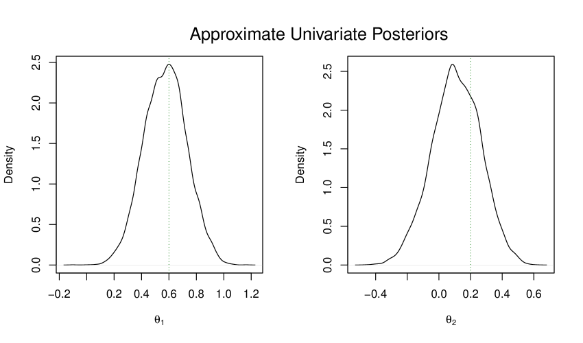
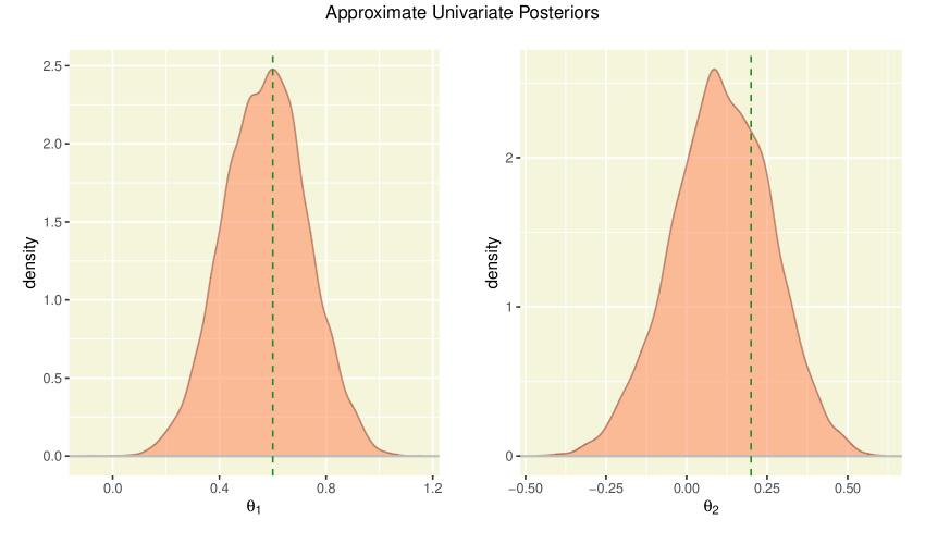
The plot function for BSL draws the approximate univariate posterior distribution for each parameter with either the default R graphics (Figure 3) or ggplot2 (Figure 4).
R> plot(resultMa2BSL, which = 1, thetaTrue = c(0.6, 0.2), thin = 30)R> mtext(’Approximate Univariate Posteriors’, line = 1, cex = 1.5)
R> plot(resultMa2BSL, which = 2, thetaTrue = c(0.6, 0.2), thin = 30,+ options.density = list(color = ’coral4’, fill = ’coral’, alpha = 0.5),+ options.theme = list(panel.background = element_rect(fill = ’beige’),+ plot.margin = grid::unit(rep(0.05,4), "npc")))
It is often of interest to compare multiple bsl results at the same time, for example, the following code summarises the BSL, uBSL, semiBSL, BSL with graphical lasso and BSL with Warton results.
R> results <- list(resultMa2BSL, resultMa2uBSL, resultMa2SemiBSL,+ resultMa2BSLasso, resultMa2BSLWarton)R> labels <- c(’bsl’, ’uBSL’, ’semiBSL’, ’bslasso’, ’bslWarton’)R> names(results) <- labelsR> t(sapply(results, summary))
n acc. rate (\\%) ESS theta[1] ESS theta[2]bsl 500 14 5530 5128uBSL 500 14 5023 5368semiBSL 500 13 4874 5075bslasso 300 28 8436 8038bslWarton 300 31 9423 7319
It can be seen that BSL, uBSL and semiBSL have very similar acceptance rates and ESS values, which indicates that their performance is very close. Both shrinkage methods increase the acceptance rate and ESS with smaller compared to BSL.
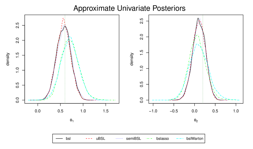
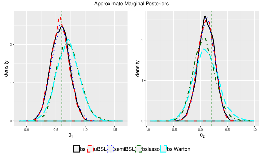
The function combinePlotsBSL plots multiple approximate posterior distributions in the same figure. The arguments are similar to the plot function of BSL, except the object to be plotted should be a list of multiple BSL objects. Figure 5 and 6 give an example of the combinePlotsBSL function.
R> par(mar = c(5, 4, 1, 2), oma = c(0, 1, 2, 0))R> combinePlotsBSL(results, which = 1, thetaTrue = c(0.6, 0.2), thin = 30,+ col = c(’black’, ’red’, ’blue’, ’green’, ’cyan’), lty = 1:5, lwd = 1)R> mtext(’Approximate Univariate Posteriors’, outer = TRUE, cex = 1.5)
R> combinePlotsBSL(results, which = 2, thetaTrue = c(0.6, 0.2), thin = 30,+ options.color = list(values=c(’black’, ’red’, ’blue’, ’darkgreen’, ’cyan’)),+ options.linetype = list(values = 1:5),+ options.size = list(values = rep(1, 5)),+ options.theme = list(plot.margin = grid::unit(rep(0.03,4), "npc"),+ axis.title = ggplot2::element_text(size=12),+ axis.text = ggplot2::element_text(size = 8),+ legend.text = ggplot2::element_text(size = 12)))
3.5 Selecting the Penalty Parameter for Shrinkage
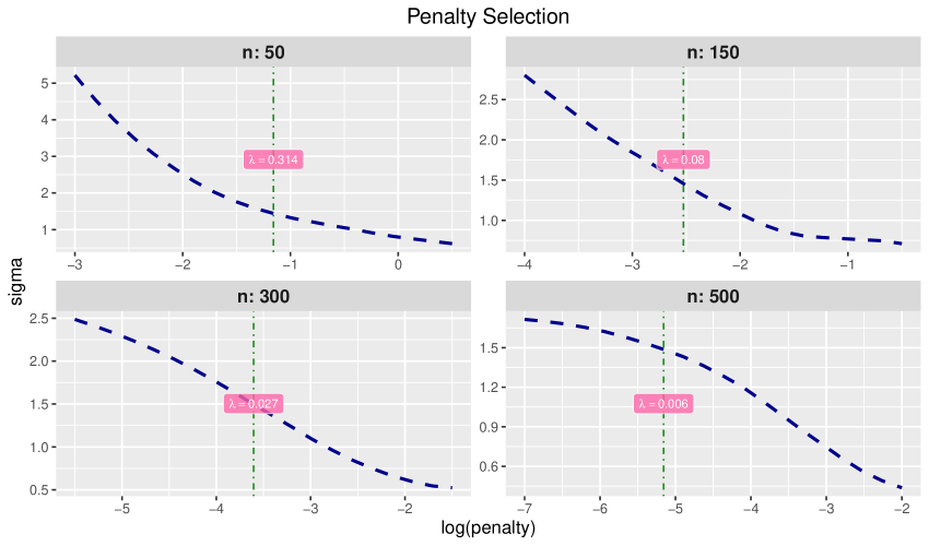
If shrinkage is desired in estimating the SL, the corresponding penalty parameter value must be selected prior to running the bsl function. This can be done via the selectPenalty function. Multiple choices for the number of simulations can be tested at the same time; simulations from the largest value of are re-used for smaller values of by subsetting. The basic arguments of selectPenalty include the summary statistic of the observed data ssy; a vector of the number of simulations to test; a list of the candidate penalty values lambda_all corresponding to each ; a point estimate of the parameter theta; the number of repeats M; the target standard deviation sigma; the model of interest model; the SL estimator method and the shrinkage estimation method shrinkage. Example code is given below (Figure 7) for selecting the of glasso with the standard BSL estimator for the MA(2) example.
R> ssy <- ma2_sum(ma2$data)R> lambda_all <- list(exp(seq(-3, 0.5, length.out = 20)),+ exp(seq(-4, -0.5, length.out = 20)),+ exp(seq(-5.5, -1.5, length.out = 20)),+ exp(seq(-7, -2, length.out = 20)))R> set.seed(100)R> sp_bsl_glasso_ma2 <- selectPenalty(ssy = ssy, n = c(50, 150, 300, 500),+ lambda_all, theta = c(0.6, 0.2), M = 100, sigma = 1.5, model = model,+ method = ’BSL’, shrinkage = ’glasso’)
The result is of S3 class penbsl. This class has support for print and plot functions.
R> print(sp_bsl_glasso_ma2)
Call:selectPenalty(ssy = ssy, n = c(50, 150, 300, 500), lambda_all = lambda_all, theta = ma2$start, M = 100, sigma = 1.5, model = model, method = "BSL", shrinkage = "glasso")Penalty selected based on the standard deviation of the loglikelihood: n penalty sigma11 50 0.31415 1.4429 150 0.07995 1.4650 300 0.02718 1.5068 500 0.00575 1.49
R> plot(sp_bsl_glasso_ma2)
4 Summary and Future Work
This paper has presented the first comprehensive software package for Bayesian synthetic likelihood methods. It implements three different types of synthetic likelihood estimators (standard, unbiased and semi-parametric) and includes functionality for two different types of shrinkage covariance estimators to reduce the number of required model simulations. The package includes functions for extracting useful statistics and visualisations of the results after running bsl. It also includes several built-in examples to illustrate the functionality of the package.
Apart from the MA(2) example described in Section 3, the package also include two other examples: a discrete-time stochastic cell biology model, cell; and a financial model for currency exchange data, mgnk. The former example features a high dimensional summary statistic, while the latter example has a relatively large number of parameters. Additional descriptions and example code can be found in the package help link. We plan to add additional applications in a future release, including real data.
In a future release we plan to incorporate the methods of Frazier and Drovandi, (2019), which allows BSL to be much more computationally efficient when the model is misspecified, in particular when the model is unable to recover the observed value of the summary statistic. All of the methods in our BSL package use MCMC to explore the parameter space, and can thus be slow when model simulation is computationally intensive and there is a large number of parameters. Future research for this package could consider incorporating the variational Bayes synthetic likelihood methods (Tran et al., , 2017; Ong et al., 2018b, ), which scale to a large number of summary statistics and/or parameters at the expense of assuming a multivariate normal approximation of the posterior.
We welcome R developers from worldwide to help contribute to the BSL package. We have made the source code available at https://github.com/cran/BSL to allow other researchers to contribute to the BSL package.
Computational details
The results in this paper were obtained using R 3.5.3 with the BSL 3.0.0 package. R itself and all packages used are available from the Comprehensive R Archive Network (CRAN) at https://CRAN.R-project.org/.
Acknowledgments
CD was supported by an Australian Research Council’s Discovery Early Career Researcher Award funding scheme (DE160100741). ZA was supported by a scholarship under CDs grant DE160100741 and a top-up scholarship from the Australian Research Council Centre of Excellence for Mathematical and Statistics Frontiers (ACEMS). LFS would like to acknowledge support from QUT, ACEMS and EPSRC grant EP/S00159X/1. Computational resources and services used in this work were provided by the HPC and Research Support Group, Queensland University of Technology, Brisbane, Australia.
References
- An et al., (2018) An, Z., Nott, D. J., and Drovandi, C. (2018). Robust Bayesian synthetic likelihood via a semi-parametric approach. arXiv preprint arXiv:1809.05800v1.
- An et al., (2019) An, Z., South, L. F., Nott, D. J., and Drovandi, C. C. (2019). Accelerating Bayesian synthetic likelihood with the graphical lasso. Journal of Computational and Graphical Statistics, 28(2):471–475.
- Barbu et al., (2018) Barbu, C. M., Sethuraman, K., Billig, E. M. W., and Levy, M. Z. (2018). Two-scale dispersal estimation for biological invasions via synthetic likelihood. Ecography, 41(4):661–672.
- Blum and François, (2010) Blum, M. G. B. and François, O. (2010). Non-linear regression models for approximate Bayesian computation. Statistics and Computing, 20(1):63–73.
- Boudt et al., (2012) Boudt, K., Cornelissen, J., and Croux, C. (2012). The Gaussian rank correlation estimator: Robustness properties. Statistics and Computing, 22(2):471–483.
- Csillery et al., (2012) Csillery, K., Francois, O., and Blum, M. G. B. (2012). abc: an R package for approximate Bayesian computation (ABC). Methods in Ecology and Evolution.
- Del Moral et al., (2006) Del Moral, P., Doucet, A., and Jasra, A. (2006). Sequential Monte Carlo samplers. Journal of the Royal Statistical Society: Series B (Statistical Methodology), 68(3):411–436.
- Doucet et al., (2015) Doucet, A., Pitt, M. K., Deligiannidis, G., and Kohn, R. (2015). Efficient Implementation of Markov Chain Monte Carlo When Using an Unbiased Likelihood Estimator. Biometrika, 102(2):295–313.
- Drovandi et al., (2015) Drovandi, C. C., Pettitt, A. N., and Lee, A. (2015). Bayesian indirect inference using a parametric auxiliary model. Statist. Sci., 30(1):72–95.
- Dutta et al., (2017) Dutta, R., Schoengens, M., Ummadisingu, A., Widmer, N., Onnela, J.-P., and Mira, A. (2017). ABCpy: A high-performance computing perspective to approximate Bayesian computation. arXiv preprint arXiv:1711.04694v2.
- Eddelbuettel, (2013) Eddelbuettel, D. (2013). Seamless R and C++ Integration with Rcpp. Springer.
- Eddelbuettel and Francois, (2011) Eddelbuettel, D. and Francois, R. (2011). Rcpp: Seamless R and C++ integration. Journal of Statistical Software, Articles, 40(8):1–18.
- Everitt, (2017) Everitt, R. G. (2017). Bootstrapped synthetic likelihood. arXiv preprint arXiv:1711.05825v2.
- Fasiolo and Wood, (2014) Fasiolo, M. and Wood, S. (2014). An Introduction to synlik (2014). R package version 0.1.0.
- Frazier and Drovandi, (2019) Frazier, D. T. and Drovandi, C. (2019). Robust approximate Bayesian inference with synthetic likelihood. arXiv preprint arXiv:1904.04551.
- Friedman et al., (2008) Friedman, J., Hastie, T., and Tibshirani, R. (2008). Sparse inverse covariance estimation with the graphical lasso. Biostatistics, 9(3):432–441.
- Friedman et al., (2018) Friedman, J., Hastie, T., and Tibshirani, R. (2018). glasso: Graphical Lasso: Estimation of Gaussian Graphical Models. R package version 1.10.
- Ghurye and Olkin, (1969) Ghurye, S. G. and Olkin, I. (1969). Unbiased estimation of some multivariate probability densities and related functions. Ann. Math. Statist., 40(4):1261–1271.
- Izenman, (1991) Izenman, A. J. (1991). Recent developments in nonparametric density estimation. Journal of the American Statistical Association, 86(413):205–224.
- Jabot et al., (2013) Jabot, F., Faure, T., and Dumoulin, N. (2013). EasyABC: Performing efficient approximate Bayesian computation sampling schemes using R. Methods in Ecology and Evolution, 4(7):684–687.
- Karabatsos, (2018) Karabatsos, G. (2018). On Bayesian testing of additive conjoint measurement axioms using synthetic likelihood. Psychometrika, 83(2):321–332.
- Kassambara, (2019) Kassambara, A. (2019). ggcorrplot: Visualization of a Correlation Matrix using ‘ggplot2’. R package version 0.1.3.
- Magnusson and Stewart, (2014) Magnusson, A. and Stewart, I. (2014). plotMCMC: MCMC Diagnostic Plots. R package version 2.0-0.
- Microsoft Corporation and Weston, (2017) Microsoft Corporation and Weston, S. (2017). foreach: Provides Foreach Looping Construct for R. R package version 1.4.4.
- Microsoft Corporation and Weston, (2018) Microsoft Corporation and Weston, S. (2018). doParallel: Foreach Parallel Adaptor for the ‘parallel’ Package. R package version 1.0.14.
- Nott et al., (2019) Nott, D. J., Drovandi, C., and Kohn, R. (2019). Bayesian inference using synthetic likelihood: Asymptotics and adjustments. arXiv preprint arXiv:1902.04827.
- (27) Ong, V. M.-H., Nott, D. J., Tran, M.-N., Sisson, S. A., and Drovandi, C. C. (2018a). Likelihood-free inference in high dimensions with synthetic likelihood. Computational Statistics & Data Analysis, 128:271 – 291.
- (28) Ong, V. M. H., Nott, D. J., Tran, M.-N., Sisson, S. A., and Drovandi, C. C. (2018b). Variational Bayes with synthetic likelihood. Statistics and Computing, 28(4):971–988.
- Plummer et al., (2006) Plummer, M., Best, N., Cowles, K., and Vines, K. (2006). CODA: Convergence diagnosis and output analysis for mcmc. R News, 6(1):7–11.
- Price et al., (2018) Price, L. F., Drovandi, C. C., Lee, A., and Nott, D. J. (2018). Bayesian synthetic likelihood. Journal of Computational and Graphical Statistics, 27:1–11.
- Sisson et al., (2018) Sisson, S. A., Fan, Y., and Beaumont, M. (2018). Handbook of Approximate Bayesian Computation. Chapman and Hall/CRC, 1st edition.
- Tran et al., (2017) Tran, M.-N., Nott, D. J., and Kohn, R. (2017). Variational Bayes with intractable likelihood. Journal of Computational and Graphical Statistics, 26(4):873–882.
- Warton, (2008) Warton, D. I. (2008). Penalized normal likelihood and ridge regularization of correlation and covariance matrices. Journal of the American Statistical Association, 103(481):340–349.
- Wood, (2010) Wood, S. N. (2010). Statistical inference for noisy nonlinear ecological dynamic systems. Nature, 466:1102–1107.