Buffer gas cooling of a trapped ion to the quantum regime

Abstract

Great advances in precision quantum measurement have been achieved with trapped ions and atomic gases at the lowest possible temperatures Ludlow et al. (2015); Bernien et al. (2017); Zhang et al. (2017). These successes have inspired ideas to merge the two systems Tomza et al. (2019). In this way one can study the unique properties of ionic impurities inside a quantum fluid Zipkes et al. (2010); Schmid et al. (2010); Ratschbacher et al. (2013); Meir et al. (2016); Kleinbach et al. (2018); Sikorsky et al. (2018); Haze et al. (2018) or explore buffer gas cooling of the trapped ion quantum computer Daley et al. (2004). Remarkably, in spite of its importance, experiments with atom-ion mixtures remained firmly confined to the classical collision regime Schmid et al. (2018). We report a collision energy of 1.15(0.23) times the $s$-wave energy (or 9.9(2.0) $\mu$K) for a trapped ytterbium ion in an ultracold lithium gas. We observed a deviation from classical Langevin theory by studying the spin-exchange dynamics, indicating quantum behavior in the atom-ion collisions. Our results open up numerous opportunities, such as the exploration of atom-ion Feshbach resonances Idziaszek et al. (2011); Tomza et al. (2015), in analogy to neutral systems Chin et al. (2010).

Neutral buffer gas cooling of trapped ions has a long history Wesenberg et al. (1995), dating back to the times when laser cooling was still in its infancy. The development of atom trapping spurred efforts to employ quantum degenerate buffer gases. These are readily prepared in the 100 nK regime by evaporative cooling, making them superb coolants. Despite this, it is well-known that the time-dependent electric potential of a Paul trap complicates matters Major and Dehmelt (1968). It causes a fast driven motion in the ions called micromotion from which energy can be released when an ion collides with an atom. This leads to a situation in which the kinetic energy of the ion becomes much larger than that of the surrounding buffer gas. This kept buffer gas cooling uncompetitive compared to laser cooling of the ions. It has also prevented the study of interacting ions and atoms in the quantum regime and reported collision energies of atom-ion mixtures have been at least two orders of magnitude higher than the $s$-wave energy Schmid et al. (2018). It was suggested that this effect can be mitigated by employing an ion-atom combination with a large mass ratio Cetina et al. (2012) such as Yb⁺ and ⁶Li.

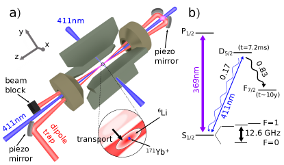
Figure 1: Setup. a) A cloud of ultracold ⁶Li atoms is prepared in an optical trap $\sim$ 50 $\mu$m below a single ion in a Paul trap (shown in gray). The ion is then immersed in the atomic cloud by transporting the atom trap up using piezo-controlled mirrors. b) After a variable atom-ion interaction time, the ion is interrogated by coupling the $S_{1/2}$ ground state on a narrow quadrupole transition to the $D_{5/2}$ excited state. The coupling strength on the transition can be directly related to the temperature of the ion. State-selective fluorescence detection allows us to establish the average coupling strength.

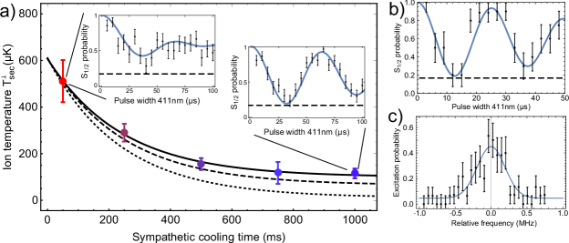
Figure 2: Cooling dynamics of an ion in the ultracold buffer gas. a) Ion temperature as a function of atom-ion interaction time together with an exponential fit (solid line) and molecular dynamics simulations with and without taking the time-dependence of the Paul trap into account (dashed and dotted lines, respectively). Before buffer gas cooling, the temperature of the ion is close to the Doppler laser cooling limit. This results in a rapidly decaying Rabi oscillation as a function of laser interrogation pulse width (inset). After buffer gas cooling, the Rabi oscillations persist for much longer. The branching ratio of decay out of the $D_{5/2}$ state limits the contrast of the Rabi oscillations to 0.83 as indicated by the dashed horizontal lines. Measurement of radial ($T_{\text{sec}}^{\perp}=42(19)\,\mu$K)(b) and axial ($T_{\text{sec}}^{\text{ax}}=130(35)\,\mu$K)(c) temperatures after 1 s of interaction time with an atomic cloud with $T_{\text{a}}=$ 2.3(0.4) $\mu$K and after adiabatic decompression of the radial ion trap potential. Errorbars denote the quantum projection noise for the state detection, while errorbars for temperatures denote the standard deviation obtained from the fits.

We trap and Doppler cool a single ¹⁷¹Yb⁺ ion in our Paul trap shown in Fig. 1a) and prepare a cloud of 10⁴ - 10^{5 6}Li atoms with a temperature of $T_{\text{a}}=2\,-\,10\,\mu$K in an optical dipole trap 50 $\mu$m below the trapped ion. The atoms are transported up by repositioning the dipole trap using piezo-controlled mirrors. After a variable interaction time, the ion is interrogated with a spectroscopy laser pulse at 411 nm that couples the $S_{1/2}$ ground state to the long-lived $D_{5/2}$ state as shown in Fig. 1b). We obtain the average kinetic energy of the ion by studying this laser excitation as a function of pulse width Leibfried et al. (1996); Meir et al. (2016). In particular, the Rabi frequency $\Omega$ of oscillations between the two states depends on the number of quanta $n$ present in the motion of the ion in its trap. Thermal occupation of excited states results in mixing of frequency components and thus damping of the Rabi oscillation. We fit the observed excitation to a model that assumes a thermal distribution with $\bar{n}$ motional quanta on average. From this, we obtain the ion’s secular temperature $T_{\text{sec}}^{\perp}\propto\bar{n}$ as explained in more detail in the Methods section.

We observe buffer gas cooling of the ion by temperature measurements after various hold times of the trapped ion in the ultracold cloud. The result for an atomic cloud with temperature $T_{\text{a}}=$10 $\mu$K and peak density $\rho=31(15)\times 10^{15}$ m^-3 is shown in Fig. 2a). Initially, the ion has a temperature of about $T_{\text{sec}}^{\perp}=\,$600 $\mu$K, which is close to the Doppler cooling limit. Then, the ion cools down with a $1/e$ time of $\tau_{\text{cool}}$ = 244(24) ms to a final temperature of $T_{\text{sec}}^{\perp}=$ 98(11) $\mu$K, corresponding to a mean number of motional quanta $\bar{n}=5.8(0.7)$ in the radial directions of motion. The buffer gas cooling thus outperforms Doppler cooling by about a factor of 5 in terms of attained temperature.

Note that the final ion temperature in Fig. 2a) is about an order of magnitude larger than the temperature of the buffer gas. This behaviour may be a direct consequence of the time-dependence of the ionic trapping potential DeVoe (2009); Zipkes et al. (2011); Chen et al. (2014); Rouse and Willitsch (2017); Höltkemeier et al. (2016); Meir et al. (2016), that causes energy release from the ion’s micromotion during a collision. We investigate this by comparing the observed dynamics of the ion in the buffer gas with classical molecular dynamics simulations Fürst et al. (2018) in which we draw the ion’s initial secular energy from a Maxwell-Boltzmann distribution at $T_{\text{sec}}=609\,\mu$K to match the data.

If we run the simulations assuming a static ion trapping potential for the ion (this is known as the secular approximation Berkeland et al. (1998)), we find complete thermalization, $T_{\text{sec}}\rightarrow T_{\text{a}}$ as shown by the dotted line in Fig. 2a). We improve our model by including the time-dependence of the Paul trap using parameters obtained from our experiment including all sources of micromotion as explained in the methods section. In this simulation, a final ion temperature of 43 $\mu$K is reached. When we also include the background heating rate of 85(50) $\mu$K/s that was measured in the absence of the atoms, the simulated final ion temperature reaches 63(12) $\mu$K, as shown by the dashed line in Fig. 2a). A likely explanation for the remaining discrepancy in final temperature is overestimation of the ion’s kinetic energy by neglecting other dephasing mechanisms in the Rabi oscillations, such as laser frequency noise. Quantum corrections may also play a role at the small energies we obtain Krych and Idziaszek (2015). We conclude that the temperature of the trapped ion is limited both by micromotion-induced heating during atom-ion collisions as well as the background heating rate of the ion.

To reach even lower energies in the experiment, we cool the atoms to $T_{\text{a}}$=2.3(0.4) $\mu$K and adiabatically lower the radial trap frequency for the ion from $\omega_{x}\approx\omega_{y}=2\pi\times$ 330 kHz to $\omega_{x}\approx\omega_{y}=2\pi\times$ 210 kHz at the end of 1 s of buffer gas cooling. In this way we achieve a temperature of $T_{\text{sec}}^{\perp}=$ 42(19) $\mu$K corresponding to $\bar{n}=3.7(1.4)$ as depicted in Fig. 2b).

The total kinetic energy of the ion can be written as $E_{\text{i}}=E_{\text{sec}}+E_{\text{iMM}}+E_{\text{eMM}}$, that is the secular (sec) energy and the energy due to the intrinsic (iMM) and excess micromotion (eMM). To obtain the total collision energy we have to additionally determine the axial secular temperature and the various micromotion energies.

Due to the weak confinement along the trap axis ($\omega_{z}=$ 2$\pi\times$ 130 kHz), it is more convenient to probe the excitation probability as a function of the frequency of the laser, which we now direct along the $z$-axis. Thermal motion leads to Doppler broadening of the resonance as plotted in Fig. 2c). We fit a Gaussian distribution to the data and we find $\sigma=193(26)$ kHz, corresponding to $T_{\text{sec}}^{\text{ax}}$ = 130(35) $\mu$K. The larger value compared to $T_{\text{sec}}^{\perp}$ has two reasons: Firstly, the weaker axial trap potential gives rise to a higher background heating rate (200 $\mu$K/s) and thus limits the attainable final temperature, and secondly the thermometry method is less reliable and more prone to overestimation of the temperature due to saturation broadening.

Intrinsic micromotion leads to a kinetic energy $E_{\text{iMM}}\approx k_{\text{B}}T_{\text{sec}}^{\perp}$ Berkeland et al. (1998). Excess micromotion occurs because of experimental imperfections that modify the trap potential. Details on the compensation and characterization of excess micromotion can be found in the methods section. In the experiment, we find $E_{\text{eMM}}/k_{\text{B}}\leq$ 44(13) $\mu$K.

The collision energy is given by Fürst et al. (2018):

$$E_{\text{col}}=\frac{\mu}{m_{\text{i}}}E_{\text{i}}+\frac{\mu}{m_{\text{a}}}E_{\text{a}},$$ (1)

with $m_{\text{i}}$ and $m_{\text{a}}$ the mass of the ion and atom, respectively, $\mu$ the reduced mass and $E_{\text{a}}=3k_{\text{B}}T_{\text{a}}/2$ the average kinetic energy of the atoms. Note that due to the large mass ratio, $\mu\approx m_{\text{a}}\ll m_{\text{i}}$. Taking into account the contribution of all types of motion as summarized in Table 1 results in a collision energy of $E_{\text{col}}=1.15(0.23)\times E_{s}$, with $E_{s}/k_{\text{B}}=8.6$ $\mu$K the $s$-wave collision energy Tomza et al. (2019).

Type of motion	$E_{\text{kin}}/\text{k}_{\text{B}}(\mu\text{K})$	$E_{\text{col}}/\text{k}_{\text{B}}(\mu\text{K})$
Radial secular ion	$2\times 21(9)$	$1.4(0.6)$
Intrinsic micromotion	$2\times 21(9)$	$1.4(0.6)$
Axial secular ion	$65(18)$	$2.2(0.4)$
Excess micromotion	$44(13)$	$1.5(0.4)$
Total ion energy	193(42)	6.6(1.4)
Atom temperature	$3/2\times 2.3(0.4)$	$3.3(0.6)$
Total collision energy	—	9.9(2.0)

Table 1: Measured energy budget of the trapped ion and atoms in terms of kinetic energy ($E_{\text{kin}}$) and collision energy ($E_{\text{col}}$). Errors are given in units of $\mu$K.

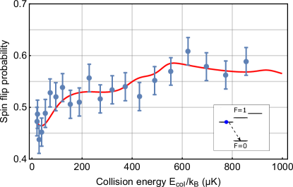
Figure 3: Spin-exchange rate versus collsion energy. Probability of detecting the ion spin in $|F=0,m_{F}=0\rangle$ after preparing it in $|F=1,m_{F}=-1\rangle$ and letting it interact with the atomic cloud for about 10 ms. The collision energy is varied using an offset field to tune the excess micromotion energy $E_{\text{eMM}}$. The red solid line is obtained by convolving the rate from quantum scattering calculations with the energy distribution of the ion as explained in the methods section. Both theory and data show a clear deviation from classical behavior in which the spin-exchange rate should be independent of collision energy. The inset shows the measured spin exchange process in the ion. Errobars denote the quantum projection noise.

Now that we cooled the mixture close to the $s$-wave limit we expect the atom-ion interactions to be governed by quantum mechanics. To look for signs of quantum behavior in the interaction we investigate the occurrence of spin-changing collisions Ratschbacher et al. (2013); Sikorsky et al. (2018); Fürst et al. (2018) as a function of collision energy. Spin-exchange is associated with short-range collisions between the atoms and ions, known as Langevin collisions. In the classical regime, the Langevin collision rate is strictly independent of collision energy Tomza et al. (2019). At very low collision energy, however, the quantization of the collision angular momentum and quantum reflection start to play a role. This leads to the occurrence of structure such as shape resonances in the spin-exchange rate. The details of this structure depend on the singlet and triplet scattering lengths that quantify the interactions between the atom and ion in the quantum regime.

After buffer gas cooling for 1 s in an atomic cloud with $T_{\text{a}}=10\,\mu$K, we prepare the ion in the state $|S_{1/2},F=1,m_{F}=-1\rangle$, with a microwave pulse. Here $F$ denotes the total angular momentum and $m_{F}$ its projection on the quantization axis. The atomic ensemble is in a spin-mixture of the lowest two Zeeman states $|S_{1/2},F=1/2,m_{F}=\pm 1/2\rangle$. Due to spin-exchange collisions during the interaction time the ion can fall to the $|S_{1/2},F=0,m_{F}=0\rangle$ state. We let the ion interact with the cloud of atoms with a density of 21(10)$\times 10^{15}$ m^-3 for about 10 ms, corresponding to about one Langevin collision. Only during the interaction time, we give the ion a variable amount of excess micromotion energy of $E_{\text{eMM}}$ by ramping offset voltages on compensation electrodes Tomza et al. (2019); Joger et al. (2017). We then shelve the population that remains in the $|S_{1/2},F=1\rangle$ state to the long lived $F_{7/2}$ state. Subsequent fluorescence detection allows to discriminate between an ion in the $|S_{1/2},F=0\rangle$ state (spin exchange) and an ion in the $F_{7/2}$ state (no spin exchange) with near unit fidelity. In Fig. 3 the result of averaging 309 of such experimental runs is shown. We see a significant dependence of the spin-exchange rate on the collision energy and thus a clear deviation from the classical prediction especially for low collision energies.

To gain further insight into the data, we compare it to multi-channel quantum scattering calculations based on the complete description of molecular and hyperfine structures. The amplitude, slope, and shape of the rate constants in the investigated energy range depend strongly on the values of the singlet and triplet scattering lengths. In Fig. 3 the calculated rate constants for the spin-exchange collisions convoluted with the experimental collision energy distribution are presented for the singlet and triplet scattering lengths of $a_{\text{S}}=1.2(0.3)R_{4}$ and $a_{\text{T}}=-1.5(0.7)R_{4}$ with $R_{4}=70$ nm Tomza et al. (2019) and 1.2(0.4) Langevin collisions on average during the interaction time. These values provide the best fit to the experimental data.

In conclusion, we have demonstrated buffer gas cooling of a single ion in a Paul trap to the quantum regime of atom-ion collisions. This has been an elusive goal in hybrid atom-ion experiments for more than a decade Tomza et al. (2019). The data and simulations suggest that even lower temperatures may be reached when using colder and denser atomic clouds, both of which are technically feasible. In particular, a denser cloud would allow eliminating the background heating rate of the ion. We speculate that controlling elastic atom-ion collisions using possible Feshbach resonances Idziaszek et al. (2011); Tomza et al. (2015) may allow tuning the cooling rate and accessible temperatures in atom-ion mixtures further, as is the case in neutral systems Chin et al. (2010).

I Methods

I.1 Determination of ion energy

To obtain information on its motional state, the ion is interrogated with a spectroscopy laser pulse at 411 nm that couples the $|S_{1/2},F=0,m_{F}=0\rangle$ state to the $|D_{5/2},F^{\prime}=2,m_{F}^{\prime}=0\rangle$ state (see Fig. 1). This state will decay to the long-lived $F_{7/2}$ state or back to the ground state with probabilities of 0.83 and 0.17, respectively Taylor et al. (1997). Subsequent fluorescence imaging allows us to detect these states with near unit fidelity. The Rabi frequency $\Omega$ of oscillations on the spectroscopy transition depends on the amount of motional quanta $n_{i}$ present in the secular motion of the ion according to $\Omega=\Omega_{0}\prod_{i=x,y,z}e^{-\eta_{i}/2}L_{n_{i}}(\eta_{i}^{2})$ Leibfried et al. (1996); Meir et al. (2016), with the ground state Rabi frequency $\Omega_{0}$, Lamb-Dicke parameter $\eta_{i}=k_{i}l^{\rm ho}$, $k_{i}$ the wavevector of the 411 nm light projected onto the direction of ion motion $i$ and $l^{\rm ho}=\sqrt{\hbar/(2m_{\rm i}\omega_{i})}$ the size of the ionic groundstate wavepacket. Here, $L_{n_{i}}(\eta_{i}^{2})$ denotes the Laguerre polynomial. Since the laser beam has a 45^∘ angle with respect to the $x$- and $y$ direction of ion motion and $\omega_{x}\approx\omega_{y}=\omega_{\perp}$, we set $\eta_{x}=\eta_{y}=\eta/\sqrt{2}$ and $\eta_{z}=0$ for the measurements on the radial motion. Thermal occupation of excited states results in mixing of frequency components and thus damping of the Rabi oscillation. To obtain the ion temperature $T_{\text{sec}}^{\perp}=\hbar\omega(\bar{n}+1/2)/k_{\text{B}}$ with $\bar{n}=(\bar{n}_{x}+\bar{n}_{y})/2$ the average number of motional quanta, we fit the observed excitation to a model that assumes a thermal distribution with $P_{\bar{n}_{x,y}}(n)=\bar{n}_{x,y}^{n}/(1+\bar{n}_{x,y})^{n+1}$ for each direction of motion $x$ and $y$. Here, we assume $\bar{n}_{x}$=$\bar{n}_{y}$.

I.2 Micromotion compensation

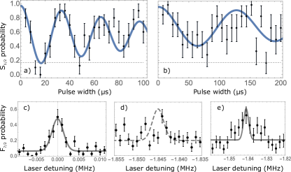
Figure 4: Micromotion analysis with resolved sideband spectroscopy. In part a) and b) Rabi oscillations on the carrier and the micromotion sideband for optimal compensation settings are plotted. From a comparison of the Rabi frequencies $\Omega_{\text{car}}=2\pi\times 32.0(0.8)\,$kHz and $\Omega_{\text{MM}}=2\pi\times 7.0(0.5)\,$kHz in combination with the applied laser powers of $P_{411}=32\,\mu$W and $P_{411}=840\,\mu$K, respectively we obtain a residual micromotion energy of $\bar{E}_{\text{eMM}}/k_{\text{B}}=21.5(1.5)\,\mu$K. Part c) shows a frequency scan over the carrier transition, carried out with a laser power of $P_{411}=61\,\mu$W. A clear peak is visible. For the data plotted in part d) the frequency of the laser is shifted by $-\Omega_{\text{rf}}=-1.85\,$MHz compared to c) and the power is increased to $P_{411}=21.7\,$mW. At the expected resonance frequency for the micromotion sideband we do not see a clear peak, only the background is higher compared to c) due to off-resonant carrier excitation at these high laser powers. If we shift the ion out of the optimal position for minimal micromotion we observe a clear resonance again as plotted in e). We conclude that the Rabi frequency $\Omega_{\text{MM}}$ on the micromotion sideband presented in e) is not larger than the Rabi frequency on the carrier $\Omega_{\text{car}}$ presented in c). From this we obtain an upper limit of the axial micromotion at the optimal position of $\bar{E}_{\text{eMM}}/k_{\text{B}}=33\,\mu$K.

The Paul trap operates at a drive frequency of $\Omega_{\text{rf}}=2\pi\times$ 1.85 MHz. The motion of an ion in the trap is composed of a secular part with eigenfrequencies $\omega_{x},\omega_{y},\omega_{z}$ and its intrinsic and excess micromotion at the drive frequency $\Omega_{\text{rf}}$. Intrinsic micromotion cannot be avoided and leads to an additional kinetic energy on the order of $E_{\text{iMM}}\sim k_{B}T_{\text{sec}}^{\perp}$ Berkeland et al. (1998). Buffer gas cooling to ultracold temperatures requires excellent control over excess micromotion. Not only does excess micromotion hinder cooling to the lowest secular temperatures as energy from the fast driven micromotion can be transferred to the secular motion of the ion during a collision with an ultracold atom, but the kinetic energy stored in the micromotion increases the overall collision energy. In the following we describe our methods to compensate micromotion to the required level. Furthermore we give a detailed analysis of the micromotion energy budget.

Stray fields

The primary cause for excess micromotion are stray electric fields, shifting the ion out of the rf-quadrupole node. We determine the remaining stray electric fields and the resulting excess micromotion with a set of two complementary methods. In horizontal direction we obtain the dc-electric field by measuring the ions position by florescence imaging on a camera as a function of radial trapping potential $\omega_{\text{rad}}$. The position shift of the ion in an electric field $E_{\text{DC}}$ is given by

$$x(\omega_{\text{rad}})=E_{\text{DC}}\times\frac{e}{m_{\text{Yb}}}\times\omega_{\text{rad}}^{-2}$$ (2)

with $e$ denoting the elementary charge and $m_{\text{Yb}}$ the mass of the Yb⁺ ion. Fitting the data, we obtain a stray field of $E_{\text{DC}}=10(10)\,$mV/m. In order to account for drifts between micromotion compensation measurements we assume a slightly higher limit of $E_{\text{DC}}\leq 50\,$mV/m. The average micromotion energy $\bar{E}_{\text{eMM}}$ is calculated as

$$\bar{E}_{\text{eMM}}(E_{\text{DC}})=\frac{E_{\text{DC}}^{2}\times e^{2}}{2m_{\text{Yb}}\times\omega_{\text{rad}}^{2}},$$ (3)

resulting in an excess micromotion energy of $\bar{E}_{\text{eMM}}/k_{\text{B}}\leq 4.7\,\mu$K ($\bar{E}_{\text{eMM}}/k_{\text{B}}\leq 1.9\,\mu$K) for a radial potential of $\omega_{\text{rad}}=2\pi\times 210$ kHz ($\omega_{\text{rad}}=2\pi\times 330$ kHz).

In vertical direction we measure stray fields using microwave Ramsey spectroscopy on the (${}^{2}S_{1/2},F=0)\leftrightarrow(^{2}S_{1/2},F=1,m_{F}=1$) transition. We apply a magnetic field gradient of $g_{v}=0.17$ T/m leading to a frequency shift of the transition by 2.3 kHz/$\mu$m. We determine the ion shift for radial potentials of $\omega_{\text{rad}}=2\pi\times 25\,$kHz and $\omega_{\text{rad}}=2\pi\times 330\,$kHz. From a linear fit to the measured frequency shifts we obtain the required compensation voltage $V_{\text{comp}}$ with an uncertainty of 0.05 V. To account for daily drifts we assume a miscompensation of $V_{\text{comp}}\leq$ 0.2 V. We obtain the micromotion energy due to this miscompensation by calibrating the energy scale with resolved sideband spectroscopy on the narrow ${}^{2}S_{1/2}\leftrightarrow^{2}D_{5/2}$ transition as explained below. For a radial potential of $\omega_{\text{rad}}=2\pi\times 210$ kHz, we obtain $\bar{E}_{\text{eMM}}/k_{\text{B}}\leq 8.3\,\mu$K.

Energy calibration

Type of micromotion	$\bar{E}_{\text{eMM}}(\text{210kHz})/k_{\text{B}}(\mu\text{K})$	$\bar{E}_{\text{eMM}}(\text{330kHz})/k_{\text{B}}(\mu\text{K})$
Axial	$13(13)$	$33(33)$
Radial Quadrature	$2\times 8.7(0.6)$	$2\times 21.5(1.5)$
Radial field (vertical)	$\leq 8.3$	$\leq 3.4$
Radial field (horizonatal)	$\leq 4.7$	$\leq 2.1$
Total	$44(13)$	$82(33)$

Table 2: Measured excess micromotion budget of the trapped ion at $\omega_{\text{rad}}=210\,$kHz and $\omega_{\text{rad}}=330\,$kHz. The total obtained excess micromotion energy at $\omega_{\text{rad}}=210$ kHz is $\bar{E}_{\text{eMM}}/k_{\text{B}}=44(13)\,\mu$K. The values in brackets denote the error in $\mu$K. The error is dominated by the error of the axial micromotion measurement.

We calibrate the excess micromotion energy versus Voltage on the compensation electrodes by using resolved sideband spectroscopy on the ${}^{2}S_{1/2}\leftrightarrow^{2}D_{5/2}$ transition. We use the magnetic field insensitive $(F=0,m_{F}=0)\leftrightarrow(F=2,m_{F}=0)$ transition in ¹⁷¹Yb⁺. We compare the Rabi frequency on the micromotion sideband and the carrier at V${}_{\text{comp}}=$7 V. We obtain $\Omega_{\text{MM}}=2\pi\times 28.3(0.9)\,$kHz and $\Omega_{\text{car}}=2\pi\times 39.0(1.2)\,$kHz. Solving

$$\frac{J_{0}(\beta_{\text{MM}})}{J_{1}(\beta_{\text{MM}})}=\frac{\Omega_{\text{car}}}{\Omega_{\text{MM}}}$$ (4)

with $J_{i}$ denoting Bessel functions, yields a modulation index $\beta_{\text{MM}}=1.18$. From the modulation index we obtain the average kinetic energy as

$$\bar{E}_{\text{eMM}}=\frac{m}{4}\left(\frac{\beta_{\text{MM}}\times\Omega_{\text{rf}}}{k}\right)^{2}$$ (5)

with $k$ the projection of the wavevector on the direction of the micromotion and $\Omega_{\text{rf}}=1.85\,$MHz the drive frequency of the trap. This results in $\bar{E}_{\text{eMM}}/k_{\text{B}}=84(7)\,\mu$K/V² $\times V_{\text{comp}}^{2}$ and $\bar{E}_{\text{eMM}}/k_{\text{B}}=208(19)\,\mu$K/V² $\times V_{\text{comp}}^{2}$ for radial potentials of $\omega_{\text{rad}}=2\pi\times 330$ kHz and $\omega_{\text{rad}}=2\pi\times 210$ kHz respectively.

Quadrature micromotion

After carefully compensating any stray electric fields, we measure the remaining micromotion by resolved sideband spectroscopy. We set the radial potential to $\omega_{\text{rad}}=2\pi\times 330$ kHz. We compare the Rabi frequency on the carrier, $\Omega_{\text{car}}=2\pi\times 32.0(0.8)\,$kHz at a laser power of $P_{411}=32\,\mu$W with the Rabi frequency on the micromotion sideband $\Omega_{\text{MM}}=2\pi\times 7.0(0.5)\,$kHz at $P_{411}=840\,\mu$W. We obtain a micromotion energy of $\bar{E}_{\text{eMM}}/k_{\text{B}}=21.5(1.5)\,\mu$K. This value includes radial micromotion caused by remaining stray electric fields as well as quadrature micromotion caused by a phase difference of the rf-signal on the opposing rf-electrodes. Since we can not differentiate between these types of radial micromotion, the obtained value is an upper limit for quadrature micromotion. The laser beam propagates at an angle of $\pi/4$ with respect to the direction of quadrature micromotion so that we have to multiply the measured value by two in order to account for the full micromotion energy. Quadrature micromotion energy is proportional to the square of the trapping potential so that we get $\bar{E}_{\text{eMM}}/k_{\text{B}}=2\times 8.7(0.6)\,\mu$K for $\omega_{\text{rad}}=2\pi\times 210$ kHz.

Axial micromotion

Finite size effects of the linear Paul trap lead to a weak rf-potential in the direction of the trap axis. Thus, the oscillating electric field vanishes at one point on the axis only. We position the single ion in our trap to this point and measure an upper limit to the remaining axial micromotion. Axial micromotion can in principle be measured in the same way as described for the quadrature micromotion, using a laser beam propagating along the trap axis. However, since our axial potential is rather weak $\omega_{\text{ax}}\leq 2\pi\times 130$ kHz, and the corresponding Lamb-Dicke parameter $\eta_{\text{ax}}\geq 0.23$, we do not observe coherent oscillation when exciting with a laser beam propagating along the trap axis. In order to still measure an upper limit for axial micromotion we compare a frequency scan over the carrier at very low power $P_{411}=61\,\mu$W with a scan over the micromotion sideband at full power $P_{411}=21.7\,$mW. From the data presented in Fig. 1 we see that the transition on the micromotion sideband at these settings is not stronger than the carrier transition. From the ratio of laser powers, we calculate an upper bound to the axial micromotion of $\bar{E}_{\text{eMM}}/k_{\text{B}}=33\,\mu$K for $\omega_{\text{rad}}=2\pi\times 330$ kHz. If we reduce the radial trap potential to $\omega_{\text{rad}}=2\pi\times 210$ kHz we obtain $\bar{E}_{\text{eMM}}/k_{\text{B}}=13\,\mu$K. The obtained limits for micromotion energy at $\omega_{\text{rad}}=2\pi\times 210$ kHz and $\omega_{\text{rad}}=2\pi\times 330$ kHz are summarized in Table 2.

I.3 Tuning the collision energy

In the experiment, we tune the kinetic energy of the ion by shifting it out of the Paul trap center with an electric control field $E_{\text{DC}}$. The resulting micromotion experienced by the ion causes a coherent motion with an energy distribution for $E\leq 2\bar{E}_{\text{eMM}}(E_{\text{DC}})$:

$$P_{\bar{E}_{\text{eMM}}}(E)=\frac{1}{\pi}\frac{1}{\sqrt{E(2\bar{E}_{\text{eMM}}(E_{\text{DC}})-E)}}.$$ (6)

To compare the data to the quantum scattering calculations, we convolute the calculated spin-exchange rates $\gamma(E)$ with this energy distribution. Here, we assume a thermal offset of 20 $\mu$K and use the maximum of the distribution to label the collision energy in Fig. 3.

I.4 Molecular dynamics simulations

Figure 5: Calculated energy distribution after buffer gas cooling of the ion using the parameters from the experiment. The frequency of average secular kinetic energies is shown and fitted with a thermal distribution for a harmonic oscillator with a temperature of $T_{\text{sec}}^{\perp}=38.2$ $\mu$K. No significant deviation from the thermal distribution is found. The results shown are from 300 simulation runs. In these simulations, the secular kinetic energy of the ion was obtained by filtering out energy contributions with a frequency higher than half the trap drive frequency, $\Omega_{\text{rf}}/2$, as explained in Ref. Fürst et al. (2018).

We numerically simulate the full trapped-ion-atom system including the excess micromotion detected in our experiment. To model collisions we introduce atoms one after another at a random location on a sphere of radius $r_{0}=0.6\,\mu$m around a single ion. Each atom starts with a velocity drawn from a Maxwell-Boltzmann distribution at $T_{\text{a}}=10\,\mu$K and passes the sphere, where it can interact with the ion. We set the interaction between the atom and ion to Fürst et al. (2018):

$$V_{\text{ia}}(r)=C_{4}\left(-\frac{1}{2r^{4}}+\frac{C_{6}}{r^{6}}\right),$$ (7)

where $C_{4}=5.607$ Jm⁴ for ⁶Li/¹⁷¹Yb⁺ and we set $C_{6}=5\times 10^{-19}$ m² to account for the short range repulsion between the atom and ion. When the atom leaves the sphere, the ion’s kinetic energy (averaged over the micromotion period) is obtained, and the next atom is introduced. We obtain the average ion cooling curve by averaging 300 simulation runs, containing $N_{\text{at}}=8000$ atoms each.

We fit an exponential of the form $T^{\perp}_{\text{sec}}(n_{\text{col}})=(T_{0}-T_{\infty})e^{-n_{\text{col}}/N_{\text{eq}}}+T_{\infty}$ to the simulated cooling dynamics. From this we obtain the characteristic $1/e$ number of collisions $N_{\text{eq}}$ it takes to equilibrate and the final ion temperature $T_{\infty}$. From the average atomic flux $\phi_{\text{at}}=N_{\text{at}}/t_{\text{prop}}$ through the sphere within the total propagation time $t_{\text{prop}}$, we can translate $N_{\text{eq}}$ into the $1/e$ number of Langevin collisions $N_{\text{L,eq}}$ via

$$N_{\text{L,eq}}=2\pi\rho_{\text{sim}}\sqrt{\frac{C_{4}}{\mu}}\frac{N_{\text{eq}}}{\phi_{\text{at}}}\,.$$ (8)

Here, $\rho_{\text{sim}}=1/(4/3\pi r_{0}^{3})$ is the atomic density in the simulation. From comparing with the experimental $1/e$ cooling time $\tau_{\text{exp}}=244(24)\,$ms, we can deduce the atomic density $\rho_{\text{at}}$ in the experiment via the Langevin rate

$$\Gamma_{\text{L}}=\frac{N_{\text{L,eq}}}{\tau_{\text{exp}}}=2\pi\rho_{\text{at}}\sqrt{\frac{C_{4}}{\mu}}\,,$$ (9)

to be $\rho_{\text{at}}=24(3)\times 10^{15}\,\text{m}^{-3}$, which is in agreement with the results from absorption imaging. .

In the experiment, the buffer gas cooling is competing with ion heating caused by electric field noise. Independent measurements give a heating rate of $\gamma_{\text{heat}}=83(50)$ $\mu$K/s in the radial direction in the absence of atoms. We account for this heating by setting $dT^{\perp}_{\text{sec}}(t)/dt=-\gamma_{\text{cool}}T^{\perp}_{\text{sec}}(t)+T_{\infty}\gamma_{\text{cool}}+\gamma_{\text{heat}}$, which results in $T^{\perp}_{\text{sec}}(t)=(T_{0}-T_{\infty})e^{-\gamma_{\text{cool}}t}+T_{\infty}+\gamma_{\text{heat}}/\gamma_{\text{cool}}$ with $\gamma_{\text{heat}}/\gamma_{\text{cool}}\sim$ 20 $\mu$K.

Finally, we obtain the energy distribution of secular ion motion from the numerical simulations. It has been found DeVoe (2009); Zipkes et al. (2011); Chen et al. (2014); Rouse and Willitsch (2017); Höltkemeier et al. (2016); Meir et al. (2016) that the energy distribution of a trapped ion can deviate significantly from a thermal distribution when interacting with a buffer gas. In our calculations we do not find an observable difference with a thermal distribution for the secular motion of the ion after buffer gas cooling, as shown in Fig. 5. We attribute this result to the large mass ratio between the atoms and ion Rouse and Willitsch (2017); Meir et al. (2016).

I.5 Quantum scattering calculations

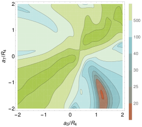
Figure 6: $\chi^{2}$ as a function of the singlet $a_{\text{S}}$ and triplet $a_{\text{T}}$ scattering lengths with the number of Langevin collisions optimized for each set of scattering lengths.

We construct and solve a quantum microscopic model of cold atom-ion interactions and collisions based on the ab initio multi-channel description of the Yb⁺-Li system as we presented in Refs. Tomza et al. (2015); Joger et al. (2017). The Hamiltonian used for the nuclear motion accounts completely for all relevant degrees of freedom including the singlet and triplet molecular electronic states, the molecular rotation, and the hyperfine and Zeeman interactions. Experimental values of relevant parameters including the magnetic field of 4 G are assumed. We construct the total scattering wave function in a complete basis set containing electronic spin, nuclear spin and rotational angular momenta.

We solve the coupled-channels equations using a renormalized Numerov propagator with step-size doubling. The wave function ratios are propagated to large interatomic separations, transformed to the diagonal basis, and the $K$ and $S$ matrices are extracted by imposing the long-range scattering boundary conditions in terms of Bessel functions. As an entrance channel, we assume Yb⁺ in the $|F=1,m_{F}=-1\rangle$ state and Li in the $|F=1/2,m_{F}=-1/2\rangle$ or $|F=1/2,m_{F}=1/2\rangle$, while all allowed other channels are included in the model. The inelastic rate constants and scattering lengths are obtained from the elements of the $S$ matrix summed over relevant channels including different partial waves $l$.

We calculate the rate constant for spin-changing collisions $K(E,a_{\text{S}},a_{\text{T}})$ as a function of the singlet $a_{\text{S}}$ and triplet $a_{\text{T}}$ scattering lengths. The scattering lengths of the singlet and triplet potentials are fixed by applying uniform scaling factors $\lambda_{i}$ to the interaction potentials: $V_{i}(R)\to\lambda_{i}V_{i}(R)$. We express scattering lengths in units of the characteristic length scale for the atom-ion interaction $R_{4}=\sqrt{\mu C_{4}/\hbar}$. Next, the rate constant is convoluted with the ion’s energy distribution induced by a controlled micromotion added to a thermal offset of $E_{0}/k_{\text{B}}$=20$\,\mu$K

$$\bar{K}(\bar{E},a_{\text{S}},a_{\text{T}})=\int_{E_{0}}^{E_{0}+\bar{E}_{\text{eMM}}}P_{\bar{E}_{\text{eMM}}}(E-E_{0})K(E,a_{\text{S}},a_{\text{T}})dE\,.$$ (10)

The probability of detecting the ion spin in $|F=0,m_{F}=0\rangle$ after preparing it in $|F=1,m_{F}=-1\rangle$ is calculated

$$S(\bar{E},a_{\text{S}},a_{\text{T}},n_{\text{L}})=1-\exp(-n_{\text{L}}\cdot\bar{K}(\bar{E},a_{\text{S}},a_{\text{T}})/K_{\text{L}})\,.$$ (11)

where $n_{\text{L}}$ is the number of Langevin collisions and $K_{\text{L}}=2\pi\sqrt{C_{4}/\mu}$ is the Langevin collision rate coefficient. The singlet and triplet scattering lengths are found together with the number of Langevin collisions by minimizing the $\chi^{2}$ function

$$\chi^{2}(a_{\text{S}},a_{\text{T}},n_{\text{L}})=\sum_{i=1}^{N_{\text{exp}}}\left(\frac{S_{\text{exp}}(\bar{E}_{i})-S(\bar{E}_{i},a_{\text{S}},a_{\text{T}},n_{\text{L}})}{\sigma_{i}}\right)^{2}\,,$$ (12)

which quantifies how well our theoretical model reproduces the measured values $S_{\text{exp}}(\bar{E}_{i})$. The numerical minimization of $\chi^{2}$ yields $a_{\text{S}}=1.2(0.3)R_{4}$, $a_{\text{T}}=-1.5(0.7)R_{4}$, and $n_{\text{L}}=1.2(0.4)$, where the uncertainties of the theoretical values are obtained by imposing that $\chi^{2}$ give the $p$-value equal or better than 0.05. Figure 6 shows corresponding $\chi^{2}$ dependence on the scattering lengths.

References

References

- Ludlow et al. (2015) A. D. Ludlow, M. M. Boyd, J. Ye, E. Peik, and P. Schmidt, Rev. Mod. Phys. 87, 637 (2015).
- Bernien et al. (2017) H. Bernien, S. Schwartz, A. Keesling, H. Levine, A. Omran, H. Pichler, S. Choi, A. S. Zibrov, M. Endres, M. Greiner, V. Vuletić, and M. D. Lukin, Nature 551, 579 (2017).
- Zhang et al. (2017) J. Zhang, G. Pagano, P. W. Hess, A. Kyprianidis, P. Becker, H. Kaplan, A. V. Gorshkov, Z.-X. Gong, and C. Monroe, Nature 551, 601 (2017).
- Tomza et al. (2019) M. Tomza, K. Jachymski, R. Gerritsma, A. Negretti, T. Calarco, Z. Idziaszek, and P. S. Julienne, Rev. Mod. Phys. 91, 035001 (2019).
- Zipkes et al. (2010) C. Zipkes, S. Paltzer, C. Sias, and M. Köhl, Nature 464, 388 (2010).
- Schmid et al. (2010) S. Schmid, A. Härter, and J. H. Denschlag, Phys. Rev. Lett. 105, 133202 (2010).
- Ratschbacher et al. (2013) L. Ratschbacher, C. Sias, L. Carcagni, J. M. Silver, C. Zipkes, and M. Köhl, Phys. Rev. Lett. 110, 160402 (2013).
- Meir et al. (2016) Z. Meir, T. Sikorsky, R. Ben-shlomi, N. Akerman, Y. Dallal, and R. Ozeri, Phys. Rev. Lett. 117, 243401 (2016).
- Kleinbach et al. (2018) K. S. Kleinbach, F. Engel, T. Dieterle, R. Löw, T. Pfau, and F. Meinert, Phys. Rev. Lett. 120, 193401 (2018).
- Sikorsky et al. (2018) T. Sikorsky, Z. Meir, R. Ben-shlomi, N. Akerman, and R. Ozeri, Nature Communications 9, 920 (2018).
- Haze et al. (2018) S. Haze, M. Sasakawa, R. Saito, R. Nakai, and T. Mukaiyama, Phys. Rev. Lett. 120, 043401 (2018).
- Daley et al. (2004) A. J. Daley, P. O. Fedichev, and P. Zoller, Phys. Rev. A 69, 022306 (2004).
- Schmid et al. (2018) T. Schmid, C. Veit, N. Zuber, R. Löw, T. Pfau, M. Tarana, and M. Tomza, Phys. Rev. Lett. 120, 153401 (2018).
- Idziaszek et al. (2011) Z. Idziaszek, A. Simoni, T. Calarco, and P. S. Julienne, New J. Phys. 13, 083005 (2011).
- Tomza et al. (2015) M. Tomza, C. P. Koch, and R. Moszynski, Phys. Rev. A 91, 042706 (2015).
- Chin et al. (2010) C. Chin, R. Grimm, P. S. Julienne, and E. Tiesinga, Rev. Mod. Phys. 82, 1225 (2010).
- Wesenberg et al. (1995) J. H. Wesenberg, R. J. Epstein, D. Leibfried, R. B. Blakestad, J. Britton, J. P. Home, W. M. Itano, J. D. Jost, E. Knill, C. Langer, R. Ozeri, S. Seidelin, and D. J. Wineland, Phys. Scr. T59, 106 (1995).
- Major and Dehmelt (1968) F. G. Major and H. G. Dehmelt, Phys. Rev. 170, 91 (1968).
- Cetina et al. (2012) M. Cetina, A. T. Grier, and V. Vuletić, Phys. Rev. Lett. 109, 253201 (2012).
- Leibfried et al. (1996) D. Leibfried, D. M. Meekhof, B. E. King, C. Monroe, W. M. Itano, and D. J. Wineland, Phys. Rev. Lett. 77, 4281 (1996).
- DeVoe (2009) R. G. DeVoe, Phys. Rev. Lett. 102, 063001 (2009).
- Zipkes et al. (2011) C. Zipkes, L. Ratschbacher, C. Sias, and M. Koehl, New J. Phys. 13, 053020 (2011).
- Chen et al. (2014) K. Chen, S. T. Sullivan, and E. R. Hudson, Phys. Rev. Lett. 112, 143009 (2014).
- Rouse and Willitsch (2017) I. Rouse and S. Willitsch, Phys. Rev. Lett. 118, 143401 (2017).
- Höltkemeier et al. (2016) B. Höltkemeier, P. Weckesser, H. López-Carrera, and M. Weidemüller, Phys. Rev. Lett. 116, 233003 (2016).
- Fürst et al. (2018) H. Fürst, N. V. Ewald, T. Secker, J. Joger, T. Feldker, and R. Gerritsma, J. Phys. B: At. Mol. Opt. Phys. 51, 195001 (2018).
- Berkeland et al. (1998) D. J. Berkeland, J. D. Miller, J. C. Bergquist, W. M. Itano, and D. J. Wineland, J. App. Phys. 83, 5025 (1998).
- Krych and Idziaszek (2015) M. Krych and Z. Idziaszek, Phys. Rev. A 91, 023430 (2015).
- Fürst et al. (2018) H. Fürst, T. Feldker, N. V. Ewald, J. Joger, M. Tomza, and R. Gerritsma, Phys. Rev. A 98, 012713 (2018).
- Joger et al. (2017) J. Joger, H. Fürst, N. Ewald, T. Feldker, M. Tomza, and R. Gerritsma, Phys. Rev. A 96, 030703(R) (2017).
- Taylor et al. (1997) P. Taylor, M. Roberts, S. V. Gateva-Kostova, R. B. M. Clarke, G. P. Barwood, W. R. C. Rowley, and P. Gill, Phys. Rev. A 56, 2699 (1997).