Abstract

In this article, we construct the diquark-antidiquark type current operators to study the axialvector $B_{c}$-like tetraquark states with the QCD sum rules. In calculations, we take the energy scale formula as a powerful constraint to choose the ideal energy scales of the QCD spectral densities and add detailed discussions to illustrate why we take the energy scale formula to improve the QCD sum rules for the doubly heavy tetraquark states. The predicted masses $M_{Z_{\bar{b}c}(1^{+-})}=7.30\pm 0.08\,\rm{GeV}$ and $M_{Z_{\bar{b}c}(1^{++})}=7.31\pm 0.08\,\rm{GeV}$ lie between the conventional $2\rm{P}$ and $3\rm{P}$ $B_{c}$ states with $J^{P}=1^{+}$ from the potential quark models, which is a typical feature of the diquark-antidiquark type $B_{c}$-like tetraquark states.

PACS number: 12.39.Mk, 12.38.Lg

Key words: Tetraquark state, QCD sum rules

1 Introduction

The mass spectrum of the $B_{c}$ mesons have been studied extensively in several theoretical approaches, such as the relativized (or relativistic) quark model with a phenomenological potential [1, 2, 3, 4], the nonrelativistic quark model with a phenomenological potential [5, 6, 7], the semi-relativistic quark model using the shifted large-$N$ expansion [8], the lattice QCD [9], the Dyson-Schwinger equation and Bethe-Salpeter equation [10], etc. Experimentally, only the ground state $B_{c}$ meson with $J^{PC}=0^{-+}$ is listed in The Review of Particle Physics [11]. Recently, the CMS collaboration observed two excited $B_{c}$ states, which are consistent with the $B_{c}(\rm 2S)$ and $B_{c}^{*}(\rm 2S)$ respectively, in the $B_{c}^{+}\pi^{+}\pi^{-}$ invariant mass spectrum in proton-proton collisions at $\sqrt{s}=13\,\rm{TeV}$ with a significance exceeding five standard deviations, the measured mass of the $B_{c}(\rm 2S)$ meson is $6871.0\pm 1.2\pm 0.8\pm 0.8\,\rm{MeV}$ [12]. Furthermore, the CMS collaboration obtained the mass gaps $M_{B_{c}(\rm 2S)}-M_{B_{c}}=596.14\pm 1.2\pm 0.8\,\rm{MeV}$ and $M_{B_{c}^{*}(\rm 2S)}-M_{B^{*}_{c}}=567.1\pm 1.0\,\rm{MeV}$ [12]. Also recently, the LHCb collaboration observed the $B_{c}^{*}(\rm 2S)$ in the $B_{c}^{+}\pi^{+}\pi^{-}$ invariant mass spectrum using proton-proton collision data at $\sqrt{s}=7$, $8$ and $13\,\rm{TeV}$, the measured mass is $6841.2\pm 0.6\pm 0.1\pm 0.8\,\rm{MeV}$ [13]. The observations of the $B_{c}(\rm 2S)$ and $B_{c}^{*}(\rm 2S)$ states have an important implication in the mass spectrum of the $B_{c}$-like tetraquark states.

In 2011, the Belle collaboration observed the $Z^{\pm}_{b}(10610)$ and $Z_{b}^{\pm}(10650)$ in the $\pi^{\pm}\Upsilon({\rm 1,2,3S})$ and $\pi^{\pm}h_{b}({\rm 1,2P})$ invariant mass spectrum firstly, and determined the favored spin-parity are $J^{P}=1^{+}$ [14], the updated masses and widths are $M_{Z_{b}(10610)}=(10607.2\pm 2.0)\,\rm{MeV}$, $M_{Z_{b}(10650)}=(10652.2\pm 1.5)\,\rm{MeV}$, $\Gamma_{Z_{b}(10610)}=(18.4\pm 2.4)\,\rm{MeV}$ and $\Gamma_{Z_{b}(10650)}=(11.5\pm 2.2)\,\rm{MeV}$, respectively [15]. The $Z^{\pm}_{b}(10610)$ and $Z_{b}^{\pm}(10650)$ are excellent candidates for the hidden-bottom tetraquark states [16, 17, 18].

In 2013, the BESIII (also the Belle) collaboration observed the $Z_{c}^{\pm}(3900)$ in the $\pi^{\pm}J/\psi$ invariant mass spectrum [19, 20]. Furthermore, the BESIII collaboration observed the $Z^{\pm}_{c}(4025)$ near the $(D^{*}\bar{D}^{*})^{\pm}$ threshold [21], and observed the $Z_{c}^{\pm}(4020)$ in the $\pi^{\pm}h_{c}$ invariant mass spectrum [22]. The $Z_{c}^{\pm}(3900)$ and $Z^{\pm}_{c}(4020/4025)$ are excellent candidates for the hidden-charm tetraquark states [23, 24, 25, 26]. For a recent comprehensive review of the $X$, $Y$, $Z$ particles both on the experimental and theoretical aspects, one can consult Ref.[27].

If the $Z_{c}^{\pm}(3900)$, $Z_{c}^{\pm}(4020/4025)$, $Z^{\pm}_{b}(10610)$ and $Z_{b}^{\pm}(10650)$) are the diquark-antidiquark type charmonium-like and bottomonium-like tetraquark states, respectively, there should exist the diquark-antidiquark type $B_{c}$-like tetraquark states. It is interesting to study this subject. At the charm sector, in 2014, the LHCb collaboration studied the $B^{0}\to\psi^{\prime}\pi^{-}K^{+}$ decays by performing a four-dimensional fit of the decay amplitude, and provided the first independent confirmation of the existence of the $Z_{c}^{-}(4430)$ state and established its spin-parity to be $J^{P}=1^{+}$ [28].

We can assign the $Z_{c}(4430)$ to be the first radial excitation of the tetraquark candidate $Z_{c}(3900)$ according to the analogous Okubo-Zweig-Iizuka supper-allowed decays,

$$Z_{c}^{\pm}(3900) \to J/\psi\pi^{\pm}\,,$$

$$Z_{c}^{\pm}(4430) \to \psi^{\prime}\pi^{\pm}\,,$$ (1)

and analogous gaps $M_{Z_{c}(4430)}-M_{Z_{c}(3900)}=591\,\rm{MeV}$ and $M_{\psi^{\prime}}-M_{J/\psi}=589\,\rm{MeV}$ [11, 30, 31, 32]. In the QCD sum rules for the $Z_{c}(3900/4020)$ as the ground state axialvector tetraquark state, it is satisfactory to choose the continuum threshold parameters as $\sqrt{s_{0}}=M_{Z_{c}}+0.50/0.55\pm 0.10\,\rm{GeV}$ [33], as the energy gaps at the charm sector have the relation $M_{Z^{\prime}_{c}}-M_{Z_{c}}=M_{\psi^{\prime}}-M_{J/\psi}$. In Ref.[34], we assume $M_{Z^{\prime}_{b}}-M_{Z_{b}}=M_{\Upsilon^{\prime}}-M_{\Upsilon}=0.55\,\rm{GeV}$ at the bottom sector, and choose the continuum threshold parameters as $\sqrt{s_{0}}=M_{Z_{b}}+0.55\pm 0.10\,\rm{GeV}$ to calculate the mass spectrum of the hidden-bottom tetraquark states with the QCD sum rules. The precise value is $M_{\Upsilon^{\prime}}-M_{\Upsilon}=0.563\,\rm{GeV}$ from the Particle Data Group [11]. For the vector $B_{c}$ mesons, $M_{B_{c}^{*}(\rm 2S)}-M_{B^{*}_{c}}=567\,\rm{MeV}$ from the CMS collaboration [12], and $M_{B_{c}^{*}(\rm 2S)}-M_{B^{*}_{c}}=566\,\rm{MeV}$ from the LHCb collaboration [13]. Now we can take the experimental data from the CMS and LHCb collaborations as input parameters and choose the continuum threshold parameters as $\sqrt{s_{0}}=M_{Z_{\bar{b}c}}+0.55\pm 0.10\,\rm{GeV}$ to study the diquark-antidiquark type $B_{c}$-like tetraquark states with the QCD sum rules.

The $Z_{b}(10610)$, $Z_{b}(10650)$, $Z_{c}(3900)$ and $Z_{c}(4020)$ are observed in the analogous decays to the final states $\pi^{\pm}h_{b}({\rm 1,2P})$, $\pi^{\pm}\Upsilon({\rm 1,2,3S})$, $\pi^{\pm}J/\psi$, $\pi^{\pm}h_{c}$, we expect that their bottom-charm cousins $Z_{\bar{b}c}$ can be observed in the $B_{c}^{*}\pi^{\pm}$ mass spectrum. Although in the decay $B_{c}^{*}\to B_{c}\gamma$, the soft photon $\gamma$ is difficult to detect so as to reconstruct the $B_{c}^{*}$ state, the partial decay width $\Gamma(B_{c}^{*}\to B_{c}\gamma)$ is about $100\,\rm{eV}$ from the QCD sum rules [35]. The mass splitting $M_{B_{c}^{*}}-M_{B_{c}}$ from the nonrelativistic renormalization group is about $46\pm 15{}^{+13}_{-0.11}\,\rm{MeV}$ [36], which can be taken into account in the uncertainty analysis.

In previous works, we observed that the calculations based on the QCD sum rules support assigning the $Z_{b}(10610)$, $Z_{b}(10650)$, $Z_{c}(3900)$ and $Z_{c}(4020)$ to be the diquark-antidiquark type axialvector tetraquark states, as there are more than one axialvector tetraquark candidates for each of those $Z_{b}$ or $Z_{c}$ states [18, 25, 33, 34, 37]. If the dominant Fock components of those $Z_{b}$ or $Z_{c}$ states are really diquark-antidiquark type tetraquark states, there should exist corresponding $B_{c}$-like tetraquark states. In this article, we study the axialvector $B_{c}$-like tetraquark states with the QCD sum rules. The observation of the $B_{c}$-like tetraquark states can shed light on the nature of those $Z_{b}$ and $Z_{c}$ states, and plays an important role in establishing the tetraquark states.

The rest of the article is arranged as follows: in Sect.2, we obtain the QCD sum rules for the masses and pole residues of the axialvector $B_{c}$-like tetraquark states; in Sect.3, we present the numerical results and detailed discussions; in Sect.4, we give a short conclusion.

2 QCD sum rules for the axialvector $B_{c}$-like tetraquark states

Firstly, we write down the two-point correlation functions $\Pi_{\mu\nu}(p)$ in the QCD sum rules,

$$\Pi_{\mu\nu}(p) = i\int d^{4}xe^{ip\cdot x}\langle 0|T\Big{\{}J_{\mu}(x)J_{\nu}^{\dagger}(0)\Big{\}}|0\rangle\,,$$ (2)

where $J_{\mu}(x)=J^{++,1}_{\pm,\mu}(x)$, $J^{+,1}_{\pm,\mu}(x)$, $J^{0,1}_{\pm,\mu}(x)$, $J^{+,0}_{\pm,\mu}(x)$,

$$J^{++,1}_{\pm,\mu}(x) = \frac{\varepsilon^{ijk}\varepsilon^{imn}}{\sqrt{2}}\Big{[}u^{Tj}(x)C\gamma_{5}c^{k}(x)\bar{d}^{m}(x)\gamma_{\mu}C\bar{b}^{Tn}(x)\pm u^{Tj}(x)C\gamma_{\mu}c^{k}(x)\bar{d}^{m}(x)\gamma_{5}C\bar{b}^{Tn}(x)\Big{]}\,,$$

$$J^{+,1}_{\pm,\mu}(x) = \frac{\varepsilon^{ijk}\varepsilon^{imn}}{2}\Big{[}\Big{(}u^{Tj}(x)C\gamma_{5}c^{k}(x)\bar{u}^{m}(x)\gamma_{\mu}C\bar{b}^{Tn}(x)-d^{Tj}(x)C\gamma_{5}c^{k}(x)\bar{d}^{m}(x)\gamma_{\mu}C\bar{b}^{Tn}(x)\Big{)}$$

$$\pm\Big{(}u^{Tj}(x)C\gamma_{\mu}c^{k}(x)\bar{u}^{m}(x)\gamma_{5}C\bar{b}^{Tn}(x)-d^{Tj}(x)C\gamma_{\mu}c^{k}(x)\bar{d}^{m}(x)\gamma_{5}C\bar{b}^{Tn}(x)\Big{)}\Big{]}\,,$$

$$J^{0,1}_{\pm,\mu}(x) = \frac{\varepsilon^{ijk}\varepsilon^{imn}}{\sqrt{2}}\Big{[}d^{Tj}(x)C\gamma_{5}c^{k}(x)\bar{u}^{m}(x)\gamma_{\mu}C\bar{b}^{Tn}(x)\pm d^{Tj}(x)C\gamma_{\mu}c^{k}(x)\bar{u}^{m}(x)\gamma_{5}C\bar{b}^{Tn}(x)\Big{]}\,,$$

$$J^{+,0}_{\pm,\mu}(x) = \frac{\varepsilon^{ijk}\varepsilon^{imn}}{2}\Big{[}\Big{(}u^{Tj}(x)C\gamma_{5}c^{k}(x)\bar{u}^{m}(x)\gamma_{\mu}C\bar{b}^{Tn}(x)+d^{Tj}(x)C\gamma_{5}c^{k}(x)\bar{d}^{m}(x)\gamma_{\mu}C\bar{b}^{Tn}(x)\Big{)}$$ (3)

$$\pm\Big{(}u^{Tj}(x)C\gamma_{\mu}c^{k}(x)\bar{u}^{m}(x)\gamma_{5}C\bar{b}^{Tn}(x)+d^{Tj}(x)C\gamma_{\mu}c^{k}(x)\bar{d}^{m}(x)\gamma_{5}C\bar{b}^{Tn}(x)\Big{)}\Big{]}\,,$$

the $i$, $j$, $k$, $m$, $n$ are color indexes, the $C$ is the charge conjugation matrix, the subscripts $\pm$ denote the positive and negative charge conjugation, respectively, the superscripts $++$, $+$, $0$ before the comma denote the electric charge, the superscripts $1$ and $0$ after the comma denote the isospin. In the isospin limit, the currents $J_{+,\mu}(x)$ (or $J_{-,\mu}(x)$) couple to the diquark-antidiquark type axialvector $B_{c}$-like tetraquark states with degenerate masses. In the present work, we choose $J_{\mu}(x)=J^{+,0}_{\pm,\mu}(x)$ for simplicity.

At the hadron side, we separate the contributions of the ground state axialvector $B_{c}$-like tetraquark states,

$$\Pi_{\mu\nu}(p) = \frac{\lambda_{Z}^{2}}{M_{Z}^{2}-p^{2}}\left(-g_{\mu\nu}+\frac{p_{\mu}p_{\nu}}{p^{2}}\right)+\cdots$$ (4)

$$= \Pi(p^{2})\left(-g_{\mu\nu}+\frac{p_{\mu}p_{\nu}}{p^{2}}\right)+\cdots\,,$$

where the pole residues $\lambda_{Z}$ are defined by

$$\langle 0|J_{\mu}(0)|Z_{\bar{b}c}(p)\rangle = \lambda_{Z}\,\varepsilon_{\mu}\,,$$ (5)

the $\varepsilon_{\mu}$ is the polarization vector.

At the QCD side, we take into account the vacuum condensates $\langle\bar{q}q\rangle$, $\langle\frac{\alpha_{s}GG}{\pi}\rangle$, $\langle\bar{q}g_{s}\sigma Gq\rangle$, $\langle\bar{q}q\rangle^{2}$, $\langle\bar{q}q\rangle\langle\frac{\alpha_{s}GG}{\pi}\rangle$, $\langle\bar{q}q\rangle\langle\bar{q}g_{s}\sigma Gq\rangle$, $\langle\bar{q}g_{s}\sigma Gq\rangle^{2}$ and $\langle\bar{q}q\rangle^{2}\langle\frac{\alpha_{s}GG}{\pi}\rangle$ in the operator product expansion according to routines in Refs.[25, 37, 38], obtain the QCD spectral densities $\rho(s)$ through dispersion relation. Then we match the hadron side with the QCD side of the components $\Pi(p^{2})$ and perform Borel transform to obtain the QCD sum rules:

$$\lambda^{2}_{Z}\,\exp\left(-\frac{M^{2}_{Z}}{T^{2}}\right)=\int_{(m_{b}+m_{c})^{2}}^{s_{0}}ds\,\rho(s)\,\exp\left(-\frac{s}{T^{2}}\right)\,,$$ (6)

where the $s_{0}$ is the continuum threshold parameter, the $T^{2}$ is the Borel parameter. The lengthy expressions of the QCD spectral densities $\rho(s)$ are neglected for simplicity. In the QCD sum rules for the tetraquark states consist of two heavy quarks and two light quarks, we have to carry out the operator product expansion up to the vacuum condensates of dimension $10$. Because there are four quark lines in the correlation functions, if each heavy quark line emits a gluon, each light quark line contributes a $\bar{q}q$ pair, we obtain a operator $\bar{q}q\bar{q}qG_{\mu\nu}G_{\alpha\beta}$ in the fixed point gauge, the operator is of dimension $10$, see Fig.1.

Figure 1: A typical Feynman diagram contributes to the vacuum condensates of dimension $10$, where the solid and dashed lines denote the light and heavy quarks, respectively.

We derive Eq.(6) with respect to $\tau=\frac{1}{T^{2}}$, and obtain the QCD sum rules for the masses,

$$M^{2}_{Z} = -\frac{\frac{d}{d\tau}\int_{(m_{b}+m_{c})^{2}}^{s_{0}}ds\rho(s)\exp\left(-\tau s\right)}{\int_{(m_{b}+m_{c})^{2}}^{s_{0}}ds\rho(s)\exp\left(-\tau s\right)}\,.$$ (7)

3 Numerical results and discussions

We choose the popular or conventional values of the vacuum condensates $\langle\bar{q}q\rangle=-(0.24\pm 0.01\,\rm{GeV})^{3}$, $\langle\bar{q}g_{s}\sigma Gq\rangle=m_{0}^{2}\langle\bar{q}q\rangle$, $m_{0}^{2}=(0.8\pm 0.1)\,\rm{GeV}^{2}$, $\langle\frac{\alpha_{s}GG}{\pi}\rangle=(0.33\,\rm{GeV})^{4}$ at the energy scale $\mu=1\,\rm{GeV}$ [39, 40, 41]. As far as the heavy quark masses are concerned, the values of the heavy quark pole masses are $\hat{m}_{c}=1.67\pm 0.07\,\rm{GeV}$ and $\hat{m}_{b}=4.78\pm 0.06\,\rm{GeV}$ from the Particle Data Group [11], which lead to the relations $2\hat{m}_{c}>M_{\eta_{c}}=2.9839\,\rm{GeV}$ and $2\hat{m}_{b}>M_{\eta_{b}}=9.399\,\rm{GeV}$. So we cannot choose the pole masses in the QCD sum rules. Now we only have one option to choose the $\overline{MS}$ masses $m_{c}(m_{c})=(1.275\pm 0.025)\,\rm{GeV}$ and $m_{b}(m_{b})=(4.18\pm 0.03)\,\rm{GeV}$ from the Particle Data Group [11]. Furthermore, we neglect the small $u$ and $d$ quark masses. Then we take into account the energy-scale dependence of the input parameters from the renormalization group equation,

$$\langle\bar{q}q\rangle(\mu) = \langle\bar{q}q\rangle({\rm 1GeV})\left[\frac{\alpha_{s}({\rm 1GeV})}{\alpha_{s}(\mu)}\right]^{\frac{12}{33-2n_{f}}}\,,$$

$$\langle\bar{q}g_{s}\sigma Gq\rangle(\mu) = \langle\bar{q}g_{s}\sigma Gq\rangle({\rm 1GeV})\left[\frac{\alpha_{s}({\rm 1GeV})}{\alpha_{s}(\mu)}\right]^{\frac{2}{33-2n_{f}}}\,,$$

$$m_{c}(\mu) = m_{c}(m_{c})\left[\frac{\alpha_{s}(\mu)}{\alpha_{s}(m_{c})}\right]^{\frac{12}{33-2n_{f}}}\,,$$

$$m_{b}(\mu) = m_{b}(m_{b})\left[\frac{\alpha_{s}(\mu)}{\alpha_{s}(m_{b})}\right]^{\frac{12}{33-2n_{f}}}\,,$$

$$\alpha_{s}(\mu) = \frac{1}{b_{0}t}\left[1-\frac{b_{1}}{b_{0}^{2}}\frac{\log t}{t}+\frac{b_{1}^{2}(\log^{2}{t}-\log{t}-1)+b_{0}b_{2}}{b_{0}^{4}t^{2}}\right]\,,$$ (8)

where $t=\log\frac{\mu^{2}}{\Lambda^{2}}$, $b_{0}=\frac{33-2n_{f}}{12\pi}$, $b_{1}=\frac{153-19n_{f}}{24\pi^{2}}$, $b_{2}=\frac{2857-\frac{5033}{9}n_{f}+\frac{325}{27}n_{f}^{2}}{128\pi^{3}}$, $\Lambda=210\,\rm{MeV}$, $292\,\rm{MeV}$ and $332\,\rm{MeV}$ for the flavors $n_{f}=5$, $4$ and $3$, respectively [11, 42]. In the present work, we study the $B_{c}$-like tetraquark states, it is better to choose the flavor $n_{f}=5$. Now we begin to discuss how to choose the ideal energy scales of the QCD spectral densities.

In the QCD sum rules for the conventional (two-quark) mesons and (three-quark) baryons, the QCD spectral densities have the form $\rho(s)\sim s^{n}$ with $n\leq 1$ for the mesons and $n\leq 2$ for the baryons in the zero quark mass limit. The convergent behavior of the operator product expansion is very good. While in the QCD sum rules for the tetraquark states, irrespective of the diquark-antidiquark type compact tetraquark states and meson-meson type molecular states, the QCD spectral densities have the form $\rho(s)\sim s^{n}$ with $n\leq 4$ in the zero quark mass limit, the convergent behavior of the operator product expansion is bad, we have to choose large Borel parameter to suppress the contributions of the higher dimensional vacuum condensates.

At the hadron side, if we choose the ”single-pole + continuum states” model to represent the hadron spectral densities to study the ground states, we have to calculate the contributions of the vacuum condensates $D(n)$ of dimension $n$ with the formula,

$$D(n) = \frac{\int_{\Delta^{2}}^{s_{0}}ds\rho_{n}(s)\exp\left(-\frac{s}{T^{2}}\right)}{\int_{\Delta^{2}}^{s_{0}}ds\rho\left(s\right)\exp\left(-\frac{s}{T^{2}}\right)}\,,$$ (9)

rather than with the formula,

$$D(n) = \frac{\int_{\Delta^{2}}^{\infty}ds\rho_{n}(s)\exp\left(-\frac{s}{T^{2}}\right)}{\int_{\Delta^{2}}^{\infty}ds\rho\left(s\right)\exp\left(-\frac{s}{T^{2}}\right)}\,,$$ (10)

where the $\Delta^{2}$ denotes the lower thresholds. For the hidden-charm or hidden-bottom tetraquark states and molecular states, the lower thresholds $\Delta^{2}=4m_{Q}^{2}$, the QCD spectral densities $\rho(s)$ also depend on the heavy quark mass $m_{Q}$ heavily, small variation of the $m_{Q}$ can lead to rather different result after carrying out the integral over $ds$, if the upper threshold $s_{0}$ is chosen. In the following, we will take the QCD sum rules for the hidden-charm (hidden-bottom) tetraquark states as an example to illustrate how to choose the ideal energy scales.

The heavy quark ($\overline{MS}$) mass $m_{Q}(\mu)$ depends on the energy scale in QCD, it is an energy scale dependent quantity, irrespective of whether or not we calculate the perturbative $\mathcal{O}(\alpha_{s},\alpha_{s}^{2},\alpha_{s}^{3},\cdots)$ corrections in a particular QCD sum rule, as the QCD sum rule in itself is a QCD approach.

We can write the correlation functions $\Pi(p^{2})$ at the QCD side as

$$\Pi(p^{2}) = \int_{4m^{2}_{Q}(\mu)}^{s_{0}}ds\frac{\rho(s,\mu)}{s-p^{2}}+\int_{s_{0}}^{\infty}ds\frac{\rho(s,\mu)}{s-p^{2}}\,,$$ (11)

which are scale independent quantities,

$$\frac{d}{d\mu}\Pi(p^{2}) = 0\,,$$ (12)

we can carry out the operator product expansion at any energy scales at which perturbative calculations are feasible. In practical calculations, we cannot calculate the perturbative corrections up to arbitrary orders, even the next-to-leading order, and have to make truncations in one way or the other. Furthermore, we have to factorize the higher dimensional vacuum condensates into lower dimensional ones paying the price of modifying the energy scale dependence, as our knowledge on the higher dimensional vacuum condensates are scarce. The truncation $s_{0}$ for the continuum contributions makes the situation even bad, as the correlation between the threshold $4m^{2}_{Q}(\mu)$ and continuum threshold $s_{0}$ is unknown. So we cannot obtain energy scale independent QCD sum rules,

$$\frac{d}{d\mu}\int_{4m^{2}_{Q}(\mu)}^{s_{0}}ds\frac{\rho(s,\mu)}{s-p^{2}} \rightarrow \frac{d}{d\mu}\int_{4m^{2}_{Q}(\mu)}^{s_{0}}ds\frac{\rho(s,\mu)}{T^{2}}\exp\left(-\frac{s}{T^{2}}\right)\neq 0\,.$$ (13)

We cannot extract the hadron (or tetraquark) masses from energy scale independent QCD sum rules, as the QCD spectral densities $\rho(s,\mu)$ depend on the energy scales, the thresholds $4m_{Q}^{2}(\mu)$ also depend on the energy scales. Even in the QCD sum rules for the (conventional) pseudoscalar $D$ and $B$ mesons, where the perturbative $\mathcal{O}(\alpha_{s}^{2})$ corrections to the perturbative terms are calculated [43], the perturbative $\mathcal{O}(\alpha_{s})$ corrections to the quark condensate terms are also calculated [44], we still cannot obtain energy scale independent QCD sum rules.

We can study the hidden-bottom or hidden-charm tetraquark states with a double-well potential model. In the heavy quark limit, the heavy quark $Q$ serves as a static well potential, which attracts the light quark $q$ to form a diquark in the color antitriplet channel. While the heavy antiquark $\overline{Q}$ serves as another static well potential, which attracts the light antiquark $\bar{q}$ to form a antidiquark in the color triplet channel. We can introduce the effective heavy quark masses ${\mathbb{M}}_{Q}$ and the virtuality $V=\sqrt{M^{2}_{X/Y/Z}-(2{\mathbb{M}}_{Q})^{2}}$ to describe those tetraquark states.

Now the QCD sum rules for the hidden-charm or hidden-bottom tetraquark states have three typical energy scales $\mu^{2}$, $T^{2}$, $V^{2}$, it is natural to choose the energy scale [18, 37],

$$\mu^{2} = V^{2}={\mathcal{O}}(T^{2})\,,$$ (14)

then we obtain the formula $\mu=\sqrt{M^{2}_{X/Y/Z}-(2{\mathbb{M}}_{Q})^{2}}$ to choose the ideal energy scales of the QCD spectral densities. At the ideal energy scales, we can enhance the pole contributions at the hadron side remarkably and improve the convergent behaviors of the operator product expansion at the QCD side remarkably. For the hidden-bottom and hidden-charm tetraquark states, we can obtain the pole contributions as large as $(40-60)\%$, or even larger. Thus we can avoid to extract the tetraquark masses at small pole contributions and obtain more reliable predictions. Otherwise, we have to resort to the ”multi-pole $+$ continuum states” model to approximate the hadronic spectral densities and postpone the continuum threshold parameters to very large values.

In the present case, there are a $c$-quark and a $b$ quark in the tetraquark states, we modify the energy scale formula to be

$$\mu = \sqrt{M^{2}_{Z}-({\mathbb{M}}_{b}+{\mathbb{M}}_{c})^{2}}\,,$$ (15)

with the updated effective heavy quark masses ${\mathbb{M}}_{b}=5.17\,\rm{GeV}$ and ${\mathbb{M}}_{c}=1.82\,\rm{GeV}$ to determine the ideal energy scales of the QCD spectral densities [34, 45]. We can rewrite the energy scale formula as $M_{Z}=\sqrt{\mu^{2}+({\mathbb{M}}_{b}+{\mathbb{M}}_{c})^{2}}$, and choose the lowest feasible energy scale $\mu=1\,\rm{GeV}$ to make a crude estimation for the masses of the axialvector $B_{c}$-like tetraquark states, $M_{Z}\geq 7.06\,\rm{GeV}$. The crude estimation is based on our previous works on the masses (and widths) of the $Z_{c}(3900)$, $Z_{c}(4020)$, $Z_{c}(4430)$, $Y(4600)$, $Z_{b}(10610)$, $Z_{b}(10650)$, etc as the diquark-antiquark type tetraquark states using the QCD sum rules [18, 25, 33, 34, 37, 45, 46, 47]. In Ref.[48], D. Ebert et al study the mass spectrum of the diquark-antidiquark type tetraquark states with two heavy quarks in the relativistic quasipotential quark model, and obtain the axialvector tetraquark masses, about $7.20-7.24\,\rm{GeV}$, which are consistent with the present estimation.

Now we search for the ideal Borel parameters $T^{2}$ and continuum threshold parameters $s_{0}$ to obey the four criteria:
$\bf 1.$ Pole dominance at the hadron side;
$\bf 2.$ Convergence of the operator product expansion at the QCD side;
$\bf 3.$ Appearance of the Borel platforms;
$\bf 4.$ Satisfying the energy scale formula,
via try and error. For the continuum threshold parameters $s_{0}$, we put an additional constraint $\sqrt{s_{0}}=M_{Z_{\bar{b}c}}+0.55\pm 0.10\,\rm{GeV}$ considering the experimental data from the CMS and LHCb collaborations [12, 13].

Although the searching process is very long, we obtain the Borel parameters (or Borel windows) $T^{2}$, continuum threshold parameters $s_{0}$, ideal energy scales of the QCD spectral densities, pole contributions, and the contributions of the vacuum condensates of dimension $10$, which are shown explicitly in Table 1. The pole contributions are about $(43-63)\%$ in the Borel windows, the central values exceed $50\%$, the pole dominance condition can be satisfied. On the other hand, the contributions of the vacuum condensates of dimension $10$ are less than $2\%$ in the Borel windows, the operator product expansion is well convergent.

Then we take into account the uncertainties of the input parameters and obtain the masses and pole residues of the axialvector $B_{c}$-like tetraquark states, which are shown explicitly in Table 2 and in Figs.2–3. From Tables 1–2, we can see that the energy scale formula $\mu=\sqrt{M^{2}_{Z}-({\mathbb{M}}_{b}+{\mathbb{M}}_{c})^{2}}$ is well satisfied. In Figs.2–3, we plot the masses and pole residues of the axialvector $B_{c}$-like tetraquark states with variations of the Borel parameters at much larger ranges than the Borel widows, in the Borel windows, the Borel platforms appear. Now the four criteria of the QCD sum rules are all satisfied. and we expect to make reasonable predictions.

The $DB^{*}$ and $D^{*}B$ thresholds are $7192\,\rm{MeV}$ and $7288\,\rm{MeV}$, respectively, the predicted masses $M_{Z_{\bar{b}c}(1^{+-})}=7.30\pm 0.08\,\rm{GeV}$ and $M_{Z_{\bar{b}c}(1^{++})}=7.31\pm 0.08\,\rm{GeV}$, which lie above the $DB^{*}$ threshold, the fall-apart decays $Z_{\bar{b}c}\to DB^{*}$ can take place kinematically, while the corresponding decays $Z_{\bar{b}c}\to D^{*}B$ can take place marginally. Although the $Z_{b}(10610)$ and $Z_{b}(10650)$ are observed in the decays $Z^{+}_{b}(10610/10650)\to\pi^{+}\Upsilon({\rm 1,2,3S})$ and $\pi^{+}h_{b}({\rm 1,2P})$, the dominant decay modes are $Z_{b}^{+}(10610)\to B^{+}\bar{B}^{*0}+\bar{B}^{0}B^{*+}$ and $Z^{+}_{b}(10650)\to B^{*+}\bar{B}^{*0}$ [50]. At the charm sector, the dominant decay modes of the corresponding hidden-charm tetraquark candidates are $Z_{c}^{\pm}(3900/3885)\to(D\bar{D}^{*})^{\pm}$ [51], and $X(3872)\to D^{*0}\bar{D}^{0}+D^{0}\bar{D}^{*0}$ [52]. We can search for the $Z_{\bar{b}c}$ states in the Okubo-Zweig-Iizuka supper-allowed decays $Z_{\bar{b}c}\to B_{c}^{*}\pi$, $B_{c}\rho$, $B_{c}^{*}\rho$, $B_{c}\pi$, $DB^{*}$ and $D^{*}B$, and compare the present predictions with the experimental data at the LHCb, Belle II, CEPC, FCC, ILC in the future, which maybe shed light on the nature of the exotic $X$, $Y$, $Z$ particles.

If we take the heavy quark limit, and choose the same hadronic coupling constants in the strong decays $Z_{c}(3900)\to J/\psi\pi$, $\eta_{c}\rho$, $D\bar{D}^{*}$, $D^{*}\bar{D}$ to study the analogous decays $Z_{\bar{b}c}(1^{+-})\to B_{c}^{*}\pi$, $B_{c}\rho$, $DB^{*}$ and $D^{*}B$ [46], we can obtain a decay width $\Gamma_{Z_{\bar{b}c}(1^{+-})}\approx 20\,\rm{MeV}$, which is much smaller than the width $370^{+70}_{-70}{}^{+70}_{-132}\,\rm{MeV}$ of the $Z_{c}(4200)$ [11, 53]. In Ref.[53], we observe that the finite width effect can be absorbed into the pole residue $\lambda_{Z_{c}(4200)}$ safely, the contributions of the scattering states cannot affect the mass $M_{Z_{c}(4200)}$ significantly, the zero width and single pole approximation works, even if $\Gamma_{Z_{\bar{b}c}(1^{++})}>\Gamma_{Z_{\bar{b}c}(1^{+-})}$.

$Z_{\bar{b}c}$	$J^{PC}$	$T^{2}(\rm{GeV}^{2})$	$\sqrt{s_{0}}(\rm GeV)$	$\mu(\rm{GeV})$	pole	$D(10)$
$[qc]_{S}[\overline{qb}]_{A}-[qc]_{A}[\overline{qb}]_{S}$	$1^{+-}$	$5.0-5.6$	$7.85\pm 0.10$	$2.10$	$(43-63)\%$	$<2\%$
$[qc]_{S}[\overline{qb}]_{A}+[qc]_{A}[\overline{qb}]_{S}$	$1^{++}$	$5.0-5.6$	$7.86\pm 0.10$	$2.15$	$(43-63)\%$	$\leq 1\%$

Table 1: The Borel windows, continuum threshold parameters, energy scales of the QCD spectral densities, pole contributions, and the contributions of the vacuum condensates of dimension $10$ for the ground state $B_{c}$-like tetraquark states.

$Z_{\bar{b}c}$	$J^{PC}$	$M_{Z}(\rm{GeV})$	$\lambda_{Z}(\rm{GeV}^{5})$
$[qc]_{S}[\overline{qb}]_{A}-[qc]_{A}[\overline{qb}]_{S}$	$1^{+-}$	$7.30\pm 0.08$	$(4.82\pm 0.71)\times 10^{-2}$
$[qc]_{S}[\overline{qb}]_{A}+[qc]_{A}[\overline{qb}]_{S}$	$1^{++}$	$7.31\pm 0.08$	$(5.05\pm 0.73)\times 10^{-2}$

Table 2: The masses and pole residues of the ground state $B_{c}$-like tetraquark states.

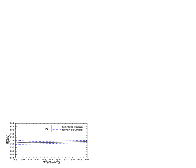
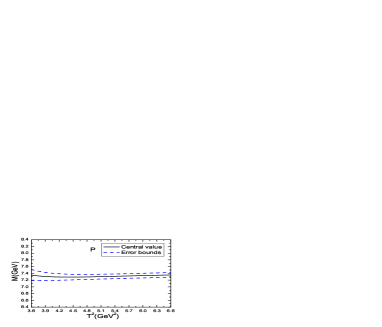
Figure 2: The masses with variations of the Borel parameters $T^{2}$ for the axialvector $B_{c}$-like tetraquark states, where the $N$ and $P$ denote the negative and positive charge conjugation, respectively.

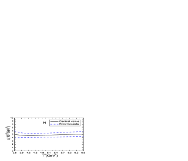
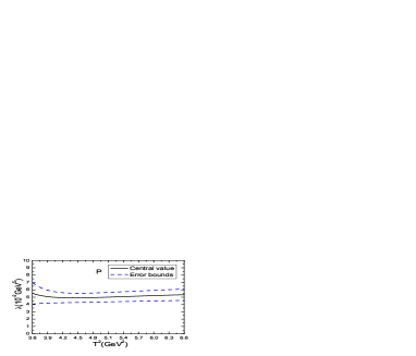
Figure 3: The pole residues with variations of the Borel parameters $T^{2}$ for the axialvector $B_{c}$-like tetraquark states, where the $N$ and $P$ denote the negative and positive charge conjugation, respectively.

The calculations based on the simple chromomagnetic interactions indicate that the lowest axialvector $B_{c}$-like tetraquark state has a mass about $6.928\,\rm{GeV}$ [49], which is below the masses $7.11-7.15\,\rm{GeV}$ for the conventional $2\rm{P}$ $B_{c}$ states with $J^{P}=1^{+}$ in the potential quark models [1, 2, 3, 4, 5, 6, 7]. The masses of the conventional $3\rm{P}$ $B_{c}$ states with $J^{P}=1^{+}$ from the potential quark models are about $7.45\,\rm{GeV}$ [4, 7]. The masses $M_{Z_{\bar{b}c}(1^{+-})}=7.30\pm 0.08\,\rm{GeV}$ and $M_{Z_{\bar{b}c}(1^{++})}=7.31\pm 0.08\,\rm{GeV}$ lie between the conventional $2\rm{P}$ and $3\rm{P}$ $B_{c}$ mesons with $J^{P}=1^{+}$, which is a typical feature of the diquark-antidiquark type $B_{c}$-like tetraquark states.

In Refs.[54, 55], the calculations based on the QCD sum rules with a different input parameter scheme indicate that the diquark-antidiquark ($6_{c}\otimes\bar{6}_{c}$) type axialvector $B_{c}$-like tetraquark states have the masses about $7.10\,\rm{GeV}$ or $7.06\,\rm{GeV}$, which differ from the present work completely, as we study the $\bar{3}_{c}\otimes 3_{c}$ type $B_{c}$-like tetraquark states.

4 Conclusion

In this article, we construct the diquark-antidiquark type current operators to study the masses and pole residues of the axialvector $B_{c}$-like tetraquark states with the QCD sum rules by carrying out the operator product expansion up to vacuum condensates of dimension $10$. In calculations, we take the energy scale formula $\mu=\sqrt{M^{2}_{Z}-({\mathbb{M}}_{b}+{\mathbb{M}}_{c})^{2}}$ as a powerful constraint to determine the ideal energy scales of the QCD spectral densities and give detailed discussions to illustrate why we take the energy scale formula to improve the QCD sum rules for the doubly heavy tetraquark states. The present predictions depend heavily on the assignments of the $Z_{c}(3900)$, $Z_{c}(4020)$, $Z_{c}(4430)$, $Y(4600)$, $Z_{b}(10610)$, $Z_{b}(10650)$, etc as the diquark-antidiquark type tetraquark states, and the experimental data about the $B_{c}^{*}(\rm 2S)$ state from the CMS and LHCb collaborations. The predicted masses $M_{Z_{\bar{b}c}(1^{+-})}=7.30\pm 0.08\,\rm{GeV}$ and $M_{Z_{\bar{b}c}(1^{++})}=7.31\pm 0.08\,\rm{GeV}$ lie between the conventional $2\rm{P}$ and $3\rm{P}$ $B_{c}$ mesons with $J^{P}=1^{+}$, which is a typical feature of the diquark-antidiquark type $B_{c}$-like tetraquark states. We can compare the present predictions with the experimental data in the future at the LHCb, Belle II, CEPC, FCC, ILC to diagnose the nature of the $X$, $Y$, $Z$ states.

References

- [1] S. Godfrey, Phys. Rev. D70 (2004) 054017.
- [2] D. Ebert, R. N. Faustov and V. O. Galkin, Phys. Rev. D67 (2003) 014027.
- [3] S. N. Gupta and J. M. Johnson, Phys. Rev. D53 (1996) 312.
- [4] J. Zeng, J. W. Van Orden and W. Roberts, Phys. Rev. D52 (1995) 5229.
- [5] S. S. Gershtein, V. V. Kiselev, A. K. Likhoded and A. V. Tkabladze, Phys. Rev. D51 (1995) 3613.
- [6] E. J. Eichten and C. Quigg, Phys. Rev. D49 (1994) 5845.
- [7] Q. Li, M. S. Liu, L. S. Lu, Q. F. Lu, L. C. Gui and X. H. Zhong, Phys. Rev. D99 (2019) 096020.
- [8] S. M. Ikhdair and R. Sever, Int. J. Mod. Phys. A20 (2005) 6509.
- [9] C. T. H. Davies et al, Phys. Lett. B382 (1996) 131.
- [10] L. Chang, M. Chen and Y. X. Liu, arXiv:1904.00399.
- [11] M. Tanabashi et al, Phys. Rev. D98 (2018) 030001.
- [12] A. M. Sirunyan et al, Phys. Rev. Lett. 122 (2019) 132001.
- [13] R. Aaij et al, Phys. Rev. Lett. 122 (2019) 232001.
- [14] I. Adachi et al, arXiv:1105.4583.
- [15] A. Bondar et al, Phys. Rev. Lett. 108 (2012) 122001.
- [16] A. Ali and C. Hambrock and W. Wang, Phys. Rev. D85 (2012) 054011.
- [17] C. Y. Cui, Y. L. Liu and M. Q. Huang, Phys. Rev. D85 (2012) 074014; S. S. Agaev, K. Azizi and H. Sundu, Eur. Phys. J. C77 (2017) 836.
- [18] Z. G. Wang and T. Huang, Nucl. Phys. A930 (2014) 63.
- [19] M. Ablikim et al, Phys. Rev. Lett. 110 (2013) 252001.
- [20] Z. Q. Liu et al, Phys. Rev. Lett. 110 (2013) 252002.
- [21] M. Ablikim et al, Phys. Rev. Lett. 112 (2014) 132001.
- [22] M. Ablikim et al, Phys. Rev. Lett. 111 (2013) 242001.
- [23] R. Faccini, L. Maiani, F. Piccinini, A. Pilloni, A. D. Polosa and V. Riquer, Phys. Rev. D87 (2013) 111102(R).
- [24] N. Mahajan, arXiv:1304.1301; E. Braaten, Phys. Rev. Lett. 111 (2013) 162003; C. F. Qiao and L. Tang, Eur. Phys. J. C74 (2014) 3122.
- [25] Z. G. Wang and T. Huang, Phys. Rev. D89 (2014) 054019.
- [26] J. M. Dias, F. S. Navarra, M. Nielsen and C. M. Zanetti, Phys. Rev. D88 (2013) 016004.
- [27] N. Brambilla, S. Eidelman, C. Hanhart, A. Nefediev, C. P. Shen, C. E. Thomas, A. Vairo and C. Z. Yuan, arXiv:1907.07583.
- [28] R. Aaij et al, Phys. Rev. Lett. 112 (2014) 222002.
- [29] M. Ablikim et al, Phys. Rev. Lett. 119 (2017) 072001.
- [30] L. Maiani, F. Piccinini, A. D. Polosa and V. Riquer, Phys. Rev. D89 (2014) 114010.
- [31] M. Nielsen and F. S. Navarra, Mod. Phys. Lett. A29 (2014) 1430005.
- [32] Z. G. Wang, Commun. Theor. Phys. 63 (2015) 325.
- [33] Z. G. Wang, arXiv:1901.10741.
- [34] Z. G. Wang, Eur. Phys. J. C79 (2019) 489.
- [35] Z. G. Wang, Eur. Phys. J. C73 (2013) 2559.
- [36] A. A. Penin, A. Pineda, V. A. Smirnov and M. Steinhauser, Phys. Lett. B593 (2004) 124.
- [37] Z. G. Wang, Eur. Phys. J. C74 (2014) 2874.
- [38] Z. G. Wang, Eur. Phys. J. C74 (2014) 2963.
- [39] M. A. Shifman, A. I. Vainshtein and V. I. Zakharov, Nucl. Phys. B147 (1979) 385.
- [40] L. J. Reinders, H. Rubinstein and S. Yazaki, Phys. Rept. 127 (1985) 1.
- [41] P. Colangelo and A. Khodjamirian, hep-ph/0010175.
- [42] S. Narison and R. Tarrach, Phys. Lett. 125 B (1983) 217.
- [43] K. G. Chetyrkin and M. Steinhauser, Phys. Lett. B502 (2001) 104; K. G. Chetyrkin and M. Steinhauser, Eur. Phys. J. C21 (2001) 319.
- [44] M. Jamin and B. O. Lange, Phys. Rev. D65 (2002) 056005; Z. G. Wang, JHEP 1310 (2013) 208; Z. G. Wang, Eur. Phys. J. C75 (2015) 427.
- [45] Z. G. Wang, Eur. Phys. J. C76 (2016) 387.
- [46] Z. G. Wang and J. X. Zhang, Eur. Phys. J. C78 (2018) 14.
- [47] Z. G. Wang, Eur. Phys. J. C79 (2019) 184.
- [48] D. Ebert, R. N. Faustov, V. O. Galkin and W. Lucha, Phys. Rev. D76 (2007) 114015.
- [49] J. Wu, X. Liu, Y. R. Liu and S. L. Zhu, Phys. Rev. D99 (2019) 014037.
- [50] A. Garmash et al Phys. Rev. Lett. 116 (2016) 212001.
- [51] M. Ablikim et al, Phys. Rev. Lett. 112 (2014) 022001.
- [52] C. Li and C. Z. Yuan, arXiv:1907.09149.
- [53] Z. G. Wang, Int. J. Mod. Phys. A30 (2015) 1550168.
- [54] W. Chen, T. G. Steele and S. L. Zhu, Phys. Rev. D89 (2014) 054037.
- [55] S. S. Agaev, K. Azizi and H. Sundu, Eur. Phys. J. C77 (2017) 321.