The switching effect of the side chain on quantum walks on triple graphs

Abstract

We consider a continuous-time quantum walk on a triple graph and investigate the influence of the side chain on the propagation in the main chain. Calculating the interchange of the probabilities between the two parts of the main chain, we find that a switching effect appears if there are odd number of points on the side chain when concrete conditions between the length of the main chain and the position of the side chain are satisfied. Whereas, such an effect does not occur if there are even number of points on the side chain. We also suggest two proposals for experiment to observe such an effect, which may be employed to design new type of switching device.

I Introduction

Although the quantum walk was proposed as the quantum mechanical counterpart of the classical random walk Ahar , it exhibits exotic features and has extensive potential applications in many fields comparing with the classical random walk. For example, the quantum walk can not only provide us a simple model to study the coherent quantum control over atoms or photons in physical systems but also offer us an advanced tool for new quantum algorithms Moh ; Shen ; Sal . So the study of the quantum walk has been receiving increasing attentions in recent years. In the context of quantum information, the continuous-time and discrete-time quantum walks were sequentially proposed Ahar ; Far with the goal of applying them to quantum algorithms. For discrete-time quantum walks, one need a quantum coin to generate a superposition state for each step. Whereas, for continuous-time quantum walks, the quantum coin is not needed and the quantum-walk process is realized through the continuous tunneling between neighbor sites, which implies that the continuous-time quantum walk can be implemented on some possible lattice sites.

The propagation features of quantum walk is obviously affected by the graph where the quantum walk is implemented. So far, the quantum walks on different graphs, such as hypercube Kem ; Kos ; Kro ; Mar ; Adi , cycle c1 ; c2 ; c3 , hypercycle hcy1 and percolation graphs p1 ; p2 ; p3 , have been widely investigated. For example, the mixing time and hitting time of quantum walks were studied in Ref. Kem ; Kos ; Kro ; Mar ; Adi where the hitting time of quantum walks for the opposite corners in the hypercube graph was shown to be exponentially faster than that of classical random walks. The upper-bound of the mixing time of quantum walks on cycle graph was also estimated in Ref.c2 . Additionally, in some literatures  gi1 ; gi2 ; gi3 ; gi4 , the quantum walk was used to distinguish the isomorphism of the graph.

Since the quantum walks on different graphs can exhibit different characters, the study of that can not only simulate some phenomena in conventional systems but also enlighten us to find more potential applications of quantum walk. Therefore we consider a continuous-time quantum walk on a triple graph in this paper. We show how the length and the position of the side chain, and the length of the main chain influence the propagation properties. Especially, we find that the quantum-walk system can exhibit obviously different propagation properties when the parity of the number of the points on the side chain is changed. This parity effect on quantum walks is expected to be used for switching devices. A similar effect was noticed in mesoscopic metal ring Ho where there is a circulating current when a magnetic flux crosses the mesoscopic metal ring. Such a circulating current can be influenced by the parity of the number of the electrons, which implies that the parity effect can exhibit in mesoscopic metal microstructures. In a word, comparing the quantum walk on one-dimensional lattices, the existence of the side chain can obviously change the propagation properties of quantum walks, therefore it is worthwhile for us to study the quantum walks on triple graphs.

This paper is organized as follows. In the next Section, we present the model of the system. In Sec. III.1, with the help of Green function we investigate the quantum walk on the triple graph with the side chain of one point and find that the system can exhibit the switching effect via changing the length of the main chain or the position of the side chain when the tunneling strength on the side chain is much larger than that on the main chain. In Sec. III.2 and Sec. III.3, we investigate the case of the side chain with two points and more points, respectively. We find that when the number of points on the side chain is even, the system can not exhibit the switching effect no matter what the length of the main chain is, which is contrast to the case of the side chain with odd points. In the last section, we propose two possible experimental schemes to observe or apply the dynamical properties exhibited in the system we considered and give a brief summary.

II Modelling quantum random walk on triple graph

We consider quantum random walks of single particle on the following triple type graph,

The graph contains a main chain of $N$ points and a side chain of $S$ points where the side chain is connected to a certain point on the main chain. It becomes more convenient for us to label the points on the main chain by $1$, $2$, $\cdots$, $N$, and the points on the side chain by $N+1$, $N+2$, $\cdots$, $N+S$. Then the graph can be equivalently plotted as

That is a one-dimensional chain of $N+S$ points with a connection broken between points $N$ and $N+1$ while with an additional ^′long-distance^′ connection between points $\ell$ and $N+1$. This implies that the point of $\ell$ is a special point that divides the main chain into two parts. Then we can model the quantum random walk on the triple type graph by the following Hamiltonian

$$H = \Bigl{(}-\sum_{j=1}^{N-1}\mid j\rangle\langle j+1\mid-J\sum_{j=N+1}^{N+S-1}\mid j\rangle\langle j+1\mid$$ (1)

$$-J\mid\ell\rangle\langle N+1\mid\Bigr{)}+~{}\mathrm{h.c.},$$

where $\mid j\rangle$ denotes the state that a particle occupies the $j$-th site on the one-dimensional lattice and $J$ the hopping strength on the side chain and that between the side chain and the $\ell$-th point of the main chain. The hopping strength on the main chain is set to unit for simplicity.

We know that the properties of continuous-time quantum walk sensitively depend on the type of graphs where the quantum walk is implemented. Although the quantum walk in one dimension has well studied, the add of the side chain can obviously change the propagation character of quantum walks. Then our main purpose is to find out how the side chain influences the state evolution on main chain by calculating of the interchange of the probabilities between the two parts of the main chain. And we further expect to use the side chain to manipulate the evolution of the probability on the main chain, which maybe enlightening for switching devices.

III Green Function and Dynamical propagation features

Let us start from the main-chain relevant part of the total Hamiltonian (1),

$$H_{\textrm{M}}=-\sum_{j=1}^{N-1}\mid j\rangle\langle j+1\mid+~{}\mathrm{h.c.}$$

We know that its eigenvalues and the eigenstates are given by

$$E_{m} = -2\cos\left(m\frac{\pi}{N+1}\right),$$

$$\mid\psi_{m}\rangle = \sum_{j=1}^{N}\sqrt{\frac{2}{N+1}}\sin\left(jm\frac{\pi}{N+1}\right)\mid j\rangle.$$ (2)

Here, $m=1$, $2$, $\cdots$, $N$, and $j=1$, $2$, $\cdots$, $N$. Then we can obtain the Green function of the main chain Hamiltonian $H_{M}$

$$g_{0}(z)=\sum_{m=1}^{N}\frac{\mid\psi_{m}\rangle\langle\psi_{m}\mid}{z+2\cos(\frac{m\pi}{N+1})}.$$ (3)

Note that when the side chain is included, the Green function of our model (1) can also be obtained. Then with the help of Green function and numerical calculation, we are mainly aim to find out how the side chain influences the state evolution on main chain by calculating of the interchange of the probabilities between the two parts of the main chain. Here the points in the left of the connection point $\ell$ (i.e., the points $j$ with $1\leq j<\ell$) are consist of the left part, and the other points in the main chain (i.e., the points $j$ with $\ell<j\leq N$) are consist of the right part. Taking the two cases of $S=1$ and $S=2$ as examples (i.e., there are one or two sites on the side chain, respectively ), we find that the propagation features for $S=1$ and $S=2$ are completely different even if the other parameters and initial states are the same. Additionally, we also show the influence of the position of the connection point $\ell$ and the number of points in the main chain on the propagation properties of the system.

III.1 Side chain with one point

Now we are in the position to consider the case of side chain with one point (i.e., $S=1$). In this case, the Green function can be written as

$$G_{1} = \frac{\mid N+1\rangle\langle N+1\mid}{z}+g_{0}+\frac{g_{0}\mid\ell\rangle\langle\ell\mid g_{0}}{z/J^{2}-\left<\ell|g_{0}|\ell\right>}$$ (4)

$$+\frac{\langle\ell\mid g_{0}\mid\ell\rangle}{z}\times\frac{\mid N+1\rangle\langle N+1\mid}{z/J^{2}-\left<\ell|g_{0}|\ell\right>}$$

$$-\frac{1}{J}\times\frac{g_{0}\mid\ell\rangle\langle N+1\mid+\mid N+1\rangle\langle\ell\mid g_{0}}{z/J^{2}-\left<\ell|g_{0}|\ell\right>}.$$

From the above Green function, one can easily obtain the eigenvalues of the Hamiltonian (1) for $S=1$. We find that the existence of the side chain with one point divides the eigenvalues of the main chain Hamiltonian $H_{\mathrm{M}}$ into two kinds. That eigenvalues of $H_{\mathrm{M}}$ remain when the corresponding eigenstates satisfy that $\langle\ell|\psi_{m}\rangle=0$ (i.e., such eigenvalues are also eigenvalues of the Hamiltonian (1) for $S=1$), while the others are shifted and no longer the eigenvalues of the Hamiltonian (1) for $S=1$ due to the existence of the side chain. Except for the remaining eigenvalues of $H_{\mathrm{M}}$, the other eigenvalues of the Hamiltonian (1) for $S=1$ can be obtained via the roots of equation $z/J^{2}-\left<\ell|g_{0}|\ell\right>=0$.

Let us see the case of $J\gg 1$ where the above equation can be solved analytically, and the corresponding roots read

$$z=\begin{cases}&z_{0}+\triangle(z_{0})\\[2.84526pt] &\pm J\end{cases},$$

$$\triangle(z_{0})=-\frac{z_{0}}{J^{2}\left<\ell|g_{0}(z_{0})^{2}|\ell\right>},$$ (5)

where $z_{0}$ is determined by $\left<\ell|g_{0}(z_{0})|\ell\right>=0$. Substituting Eq. (3) into Eq. (III.1), we can obtain the value of $z_{0}$. Then the changed energy levels can be written as

$$E_{n} = -2\cos(\frac{n\pi}{\ell}),$$ (6)

$$E_{n^{\prime}} = -2\cos(\frac{n^{\prime}\pi}{N+1-\ell}),$$ (7)

with $n=1,2,\cdots\ell-1$ and $n^{\prime}=1,2,\cdots N-\ell$. Here the perturbation term $\Delta(z_{0})\sim\frac{1}{J^{2}}$ are neglected due to the fact $J\gg 1$. From the above expressions of $E_{n(n^{\prime})}$, we can find that if $(N+1)$ and $\ell$ have the greatest common divisor larger than two, some energy levels of $E_{n}$ can be degenerate with that of $E_{n^{\prime}}$, respectively, and the corresponding values of that degeneracy energy levels are just equal to those remaining eigenvalues of $H_{\mathrm{M}}$. Whereas, if $(N+1)$ and $\ell$ have no the greatest common divisor larger than two, once the side chain with one point is included, none of the eigenvalues of $H_{\mathrm{M}}$ remain and the energy levels of $E_{n}$ and $E_{n^{\prime}}$ are not degenerate. The above expression implies that the relation between the position of the connection point and the number of points on the main chain can obviously affect the distribution of the energy levels of the system. So the propagation properties in the triple graph we considered can exhibit essentially different features for different numbers of points on main chain and the positions of the connection point.

In order to investigate the propagation features of the particle in the triple graph, let us observe the time evolution of probability amplitude. Assuming the particle is in the $j_{2}$-th site of the main chain, one can write the probability amplitude $A(j_{1},j_{2})$ for the particle being in the $j_{1}$-th site at the time $t$ as

$$A(j_{1},j_{2})=\underset{E}{\sum}\mathrm{Res}G_{1}(E,j_{1},j_{2})\exp(-iEt),$$ (8)

where $G_{1}(E,j_{1},j_{2})=\langle j_{1}\mid G_{1}(E)\mid j_{2}\rangle$ with $E$ including all the eigenvalues of the Hamiltonian (1) for $S=1$, and the sign ${}^{\prime}\mathrm{Res}^{\prime}$ stands for the residue of a function. If $j_{1}>\ell$ and $j_{2}<\ell$, the probability amplitude can be given as

$$p(j_{1},j_{2})=O(\frac{1}{J^{2}})+$$

$$\underset{E\in E_{r}}{\sum}\frac{2}{N+1}\sin[j_{1}\theta(E)]\sin[j_{2}\theta(E)]e^{(-iEt)}[e^{(-i\triangle(E)t)}-1],$$

where $E_{r}$ refer to the remaining eigenvalues of $H_{\mathrm{M}}$ ( i.e., $E_{r}$ are the energies given in Eq. (III) whose corresponding eigenstates $\mid\psi_{m}\rangle$ satisfy $\langle\ell|\psi_{m}\rangle=0$), $\theta(E)=\displaystyle\arccos(-\frac{E}{2})$ and the expression of $\Delta(E)$ is given in Eq. (III.1). From the above expression (III.1), we can find that for $J\gg 1$, the value of $p(j_{1},j_{2})$ is not zero only when there are non-zero eigenvalues of $H_{\mathrm{M}}$ remained, i.e., $(N+1)$ and $\ell$ have the greatest common divisor larger than two. So that the particle can cross the connection point from the one part into the other part of the main chain for $(N+1)$ and $\ell$ having the greatest common divisor larger than two while the particle is always in the initial part of the main chain for $(N+1)$ and $\ell$ having no greatest common divisor larger than two, which will be confirmed by Fig. 1 . Additionally, we can also obtain the probability amplitude of particle from the main chain into the side chain

$$\mathrm{Res}\langle j|G_{1}(J)|N+1\rangle=-\frac{1}{2}\delta_{j\ell}-\frac{1}{2J}\langle j|H_{\mathrm{M}}|\ell\rangle,$$ (10)

which is zero as long as the particle is not in the connection point at the initial time.

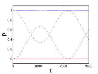
Figure 1: (color online) The time evolution of the probabilities for the particle in the two different parts of the main chain, respectively, for $S=1$. The parameters are $J=10$, $N=11$, and $\ell=5$ for the solid lines and $\ell=6$ for the dot lines.

In Fig. 1, we plot the time evolution of probabilities for particles in the left part and in the right part of the main chain, respectively, for different values of $\ell$. Note that in this and the following figures, the unit of time $t$ is in the unit of the inverse of the hopping strength on the main chain, and that of tunneling strength $J$ is in the unit of the hopping strength on the main chain. At the initial time, the particle is in the third point so that the particle is initially in the left part of the main chain. Since the probability amplitude $A(j_{1},j_{2})$ for the particle tunneling between different points is given in Eq. (III.1), the probability of the particle in the right part of the main chain at the time $t$ can be written as $\sum_{\ell<j_{1}\leq N}|A(j_{1},3)|^{2}$, and that in the left part of the main chain is $\sum_{1\leq j_{1}<\ell}|A(j_{1},3)|^{2}$. Note that once the particle is in the left part of the main chain, which concrete points that the particle is in does not affect the evolution features of the probability distribution in the two parts of the main chain. This is also true for the case of side chain with more than one points. From Fig. 1, we can find that the particle for $\ell=6$ ($N+1$ and $\ell$ having the greatest common divisor larger than two), the probabilities in the left and right parts of the main chain oscillate quasi-periodically with time. Whereas, the particle is always stay in the left part of the main chain and has no probability to cross the connection point $\ell$ into the right part of the main chain for $\ell=5$ ($N+1$ and $\ell$ having no greatest common divisor larger than two), which exhibits the switching effect of the side chain. Note that, except for the position of the connection point (i.e., the value of $\ell$), the other parameters and the initial states are all the same for the two cases.

III.2 Side chain with two points

For the Hamiltonian (1) with $S=2$, the Green function of the system is written as $G_{2}$ whose expression can be given carefully. Then the energy eigenvalues of the system can also be obtained with the help of $G_{2}$. For the case of $J\gg 1$, some energy levels of $H_{\mathrm{M}}$ also remain if $(N+1)$ and $\ell$ have the greatest common divisor larger than two, and the others are determined via the roots of

$$\frac{1}{z}+\langle\ell\mid g_{0}\mid\ell\rangle=0,$$ (11)

and are not degenerate no matter whether $(N+1)$ and $\ell$ have the greatest common divisor larger than two. In analogy to the discussion in the above subsection, we can obtain the probability amplitude of a particle from one point into another point on the main chain by calculating the residues of

$$\langle j_{1}\mid G_{2}\mid j_{2}\rangle=\langle j_{1}\mid g_{0}\mid j_{2}\rangle+\frac{\langle j_{1}\mid g_{0}\mid\ell\rangle\langle\ell\mid g_{0}\mid j_{2}\rangle}{z/J^{2}-\bigl{(}\displaystyle\frac{1}{z}+\left<\ell|g_{0}|\ell\right>\bigr{)}}.$$ (12)

Although it is difficult to give the analytical expression of the residues of Eq. (12), we can find that the summation of such residues is always not zero for any values of $(N+1)$ and $\ell$ because the non-zero energy levels near zero are also existed for the system with the side chain of two points. That implies that the particle can always cross the connection point into the other part of the main chain no matter whether $(N+1)$ and $\ell$ have the greatest common divisor larger than two, which can be confirmed by Fig. 2.

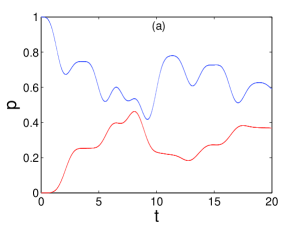
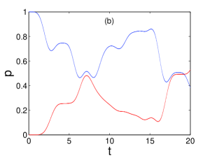
Figure 2: (color online) The time evolution of the probabilities for the particle in the two different parts of the main chain for $S=2$. The parameters are $J=10$, $N=11$, and $\ell=5$ (a), $\ell=6$ (b).

In Fig. 2, we plot the time evolution of the probability of the particle in the left and right part of the main chain, respectively. Note that we find that the probabilities of the particle in the left and right part of the main chain oscillate so fast through the numerical calculation. So in order to make Fig. 2 clear, we take a smaller time comparing to Fig. 1. At the initial time, the particle is in the left part of the main chain. From this figure, we can find that the probabilities of the particle in the two parts of the main chain oscillate with time for both $\ell=5$ and $\ell=6$, which is in contrast to the case of side chain with one point (see Fig. 1). Additionally, the oscillation of the probability is not qusi-periodical like that in Fig. 1 due to the fact that the roots of Eq. (11) are not periodical.

III.3 Side chain with more points

In the above subsections, we consider two examples of side chain with one and two points, respectively. Now, let us see the case of the side chain with more than two points. In Fig. 3, we plot the time evolution of the probability distribution in the left and right parts of the main chain, respectively, for different values of $S$. Here the value of $\ell=5$, i.e.., $N+1$ and $\ell$ have no greatest common divisor larger than two, and the particle is in the left part of the main chain at the initial time. From this figure, we can find that the particle can not cross the connection point into the other part of the main chain for $S=3$, which is in contrast to the cases of $S=4$. Meanwhile, comparing the Fig. 3 (a) with Fig. 1 , and Fig. 3 (b) with Fig. 2 (a) , respectively, we can see that the system of the side chain with odd points (even points) exhibits analogous propagation features. But the features of the system with side chain of odd points differ significantly from that of the system with side chain of even points. Such a feature can be regarded as the parity effect in the quantum walk, which can be explained with the help of Green function. The parity effect also appeared in the other physical systems, such as the mesoscopic metal ring Ho .

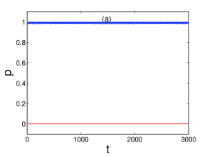
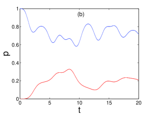
Figure 3: (color online) The time evolution of the probabilities for the particle in the two different parts of the main chain for different values of $S$. The parameters are $\ell=5$, $J=10$, $N=11$, and $S=3$ (a), $S=4$ (b).

For the system of side chain with more points, the Green function of the system can be written as

$$G_{S} = \overset{\sim}{g}_{0}+g_{0}+\frac{g_{0}\mid\ell\rangle J^{2}\times\langle N+1\mid\overset{\sim}{g}_{0}\mid N+1\rangle\langle\ell\mid g_{0}}{1-J^{2}\times\langle N+1\mid\overset{\sim}{g}_{0}\mid N+1\rangle\langle\ell\mid g_{0}\mid\ell\rangle}$$ (13)

$$+\frac{\stackrel{{\scriptstyle\sim}}{{g}}_{0}\mid N+1\rangle J^{2}\times\langle\ell\mid g_{0}\mid\ell\rangle\langle N+1\mid\stackrel{{\scriptstyle\sim}}{{g}}_{0}}{1-J^{2}\times\langle N+1\mid\overset{\sim}{g}_{0}\mid N+1\rangle\langle\ell\mid g_{0}\mid\ell\rangle}$$

$$-\frac{J\stackrel{{\scriptstyle\sim}}{{g}}_{0}\mid N+1\rangle\langle\ell\mid g_{0}+Jg_{0}\mid\ell\rangle\langle N+1\mid\stackrel{{\scriptstyle\sim}}{{g}}_{0}}{1-J^{2}\times\langle N+1\mid\overset{\sim}{g}_{0}\mid N+1\rangle\langle\ell\mid g_{0}\mid\ell\rangle},$$

where

$$\overset{\sim}{g}_{0}(z)=\frac{2}{S+1}\sum_{n=1}^{S}\frac{\mid n\rangle\langle n\mid}{z+2J\cos(\frac{n\pi}{S+1})}.$$

The same as the previous discussion, one can neglect the perturbation term of $\Delta(z_{0})$ if $J\gg 1$. Then except for the remaining energy levels of $H_{\mathrm{M}}$, the other energy levels of the system for the side chain with $S$ points are obtained

$$\begin{cases}\left<\ell|g_{0}(z_{0})|\ell\right>=0,&S=odd\\[5.69054pt] \left<\ell|g_{0}(z_{0})|\ell\right>+\displaystyle\frac{\lambda_{S}}{z_{0}}=0,&S=even\end{cases}$$ (14)

where, $\lambda_{S}=\displaystyle\frac{1}{2(S+1)}\sum_{n=1}^{S}\tan^{2}\displaystyle\frac{n\pi}{S+1}$. We can find that if the number of points on the side chain is odd, the energy levels of the system are the same as the case of $S=1$ which has been discussed in Subsec. III.1. This implies that the distribution of the energy levels for the cases of side chain with odd points are the same. Then propagation features of the particle in the triple graph for the side chain with odd points are analogous. So that all the system for the side chain with odd points can exhibit the switching effect when the number of points on the main chain and the position of the side chain satisfy concrete conditions. Additionally, for the case of $S$ being even, the distribution of the energy levels resembles the case of $S=2$ discussed in Subsec. III.2 due to the fact that the second equation in Eq. (14) are of the same kind except for the difference of the coefficient $\lambda_{S}$. So the propagation features of the particle in the triple graphs for the side chain with even points resemble each other and always do not exhibit the switching effect, which is shown in Fig. 2 (a) and Fig. 3 (b). According to the above discussion, we can find that whether the particle can go through the connection points into the other part of the main chain can be significantly influenced by the parity of the number of points on the side chain, which differs from the case studied in ref. FAR2 . In that reference, the quantum walk on a chain of points with an attached NAND tree was studied, where the transmission coefficient is determined by the evaluation results of the NAND tree. Additionally the transmission coefficient can only be zero or one. In the system we considered, we show that the probability of the particle in one part of the main chain can oscillate with time for the side chain with even points.

IV Experiment proposal and Conclusion

Since the quantum-walk system we considered can exhibit the above novel features, we expect that can be observed in experiment and even be designed as switching device. Then we propose the following possible experimental proposals. Firstly, we expect to realize such a quantum-walk system in solid systems. Assume there is a one-dimensional lattice system and the particle with spin can tunnel between nearest sites. If one applies a external magnetic field $B$ into the lattice system, the spin will be polarized to the direction of the magnetic field when the temperature is low enough. At this case, the spin degree of the particle is frozen, and then the Hamiltonian describing this system amounts to that of quantum walk in one-dimensional lattice without the side chain. Meanwhile, if one applies another magnetic field whose value and direction is equal and opposite to that of $B$, respectively, into the site $\ell$, the total magnetic field at the site $\ell$ is zero. Then once the particle tunnel into the site $\ell$, the spin degree of the particle will be released so that there is probability for the spin of the particle flipping into the another direction at the site $\ell$. Assuming the particle is an electron with spin being $1/2$, one can easily find that the Hamiltonian of this solid system is essentially equal to Eq. (1) with $S=1$. So such a system is possible to realize the quantum walk in the triple graph with the side of one point. Naturally, if the particle with spin larger than $1/2$, such system can also be used to realize the quantum walk in the triple graph with the side of more points. Note that the conventional solid system is difficult to simulate the quantum walk in the triple graph with side chain of more points because the spin of the particle in conventional solid system is usually equal to $1/2$ and difficult to reach larger values. Whereas, the cold-atom systems trapped in magnetic lattice can make up for this defect due to the fact that the spin of the particle can more various for different alkali and alkali earth metals.

The aforementioned quantum-walk system is also expected to be realized in artificial systems. For example, $N$-qubits are coupled by the single-mode resonant cavity, and the interaction Hamiltonian was given in ref. Yangsy . If at the initial time, one of the qubits is applied into a microwave pulse that is resonant with the transition between two levels of the qubit, the initial state of the $N$-qubit system is $\prod_{k\neq j}\mid\textrm{g}\rangle_{k}\mid\textrm{e}\rangle_{j}\mid 0\rangle_{\textrm{c}}$ . Such a initial state means that the $j$-th qubit is in its exited state $\mid\textrm{e}\rangle$, the others are in ground state $\mid\textrm{g}\rangle$, respectively, and the cavity mode is initially in the vacuum state $\mid 0\rangle_{\textrm{c}}$. For convenience, the initial state of the system can be written as $\mid\textrm{e}\rangle_{j}\mid 0\rangle_{\textrm{c}}$. In second-order perturbation and taking the state $\prod_{k}\mid\textrm{g}\rangle_{k}\mid 1\rangle_{\textrm{c}}$ as the medium state, the effective Hamiltonian just is the Eq. (1) without the side chain, and the Fock basis corresponding to the system can be simply denoted as a single-particle state $\mid j\rangle$ ($j=1,2,\cdots N$). Additionally, one can set up another $S$-qubits coupled by another single-mode resonant cavity as the side chain, and meanwhile couple the first qubit of the side chain with the $\ell$th qubit of the above $N$-qubits. In this case, the system can simulate the quantum-walk in the triple graph we considered. Note that the coupling strength $J$ can be tuned due to the device parameters and/or the placement of the qubits in the cavity can be changed. So the coupled-qubits system maybe more powerful to realize the quantum-walk in the triple graph we considered.

In the above, we investigated the quantum random walk on the triple type graph and show the effect of the side chain on the propagation features on the main chain. We found that if the tunneling strength on the side chain is much larger than that on the main chain, the system can exhibit the switching effect for the case of the side chain with odd points when the number of points on the main chain and the position of the side chain satisfy concrete conditions. Whereas, for the case of the side chain with even points, the particle can always pass through the connection point into the other part of the main chain no matter where the connection point between the main chain and the side chain is. So the quantum walk on the triple type graph with the side chain of even points can not exhibit the switching effect, which is contrast to the case of the side chain with odd points. Such propagation properties were explained with the help of Green function. We also suggest two proposals for experiment to observe such an effect, which is expected to be enlightening for the design of new type of switching devices.

References

- (1) Y. Aharonov, L. Davidovich, and N. Zagury, Phys. Rev. A, 48,1687 (1993).
- (2) M. Mohseni, P. Rebentrost, S. Lloyd, and A. Aspuru-Guzik, J. Chem. Phys, 129, 174106 (2008).
- (3) N. Shenvi, J. Kempe, and R.B. Whaley, Phys. Rev. A, 67,052307 (2003).
- (4) S. E. Venegas-Andraca, Quantum Information Processing 11, 1015 (2012).
- (5) E. Farhi and S. Gutmann, Phys. Rev. A, 58, 915 (1998).
- (6) J. Kempe, Probability Theory Relat.Fields, 133(2), 215 (2005).
- (7) J. Košík and V. Bužek, Phys. Rev. A, 71, 012306 (2005).
- (8) H. Krovi and T. A. Brun, Phys. Rev. A, 73, 032341(2006).
- (9) F. L. Marquezino, R. Portugal, G. Abal, and R. Donangelo, Phys. Rev. A, 77, 042312 (2008).
- (10) A. Makmal, M. Zhu, D. Manzano, M. Tiersch, and H. J. Briegel, Phys. Rev. A, 90, 022314 (2014).
- (11) M. Bednarska, A. Grudka, P. Kurzyński, T. Łuczak and A. Wójcik, Phys. Lett. A, 317, 21 (2003).
- (12) D. Solenov and L. Fedichkin, Phys. Rev. A, 73, 012313 (2006).
- (13) D. D’Alessandro, G. Parlangeli, and F. Albertini, Jour. Phys. A, 40, 14447 (2007).
- (14) D. Solenov and L. Fedichkin, Phys. Rev. A, 73, 012308 (2006).
- (15) G. Leung, P. Knott, J. Bailey and V. Kendon, New. Jour. Phys. 12, 123018 (2010).
- (16) B. Kollár, T. Kiss, J. Novotný, and I. Jex, Phys. Rev. Lett, 108, 230505 (2012)
- (17) B. Kollár, J. Novotný, T. Kiss and I. Jex, New Jour. Phys, 16, 023002 (2014).
- (18) B. L. Douglas, J. B. Wang, Jour. Phys. A, 41, 075303 (2008).
- (19) J. K. Gamble, M. Friesen, D. Zhou, R. Joynt, and S. N. Coppersmith, Phys. Rev. A, 81, 052313 (2010).
- (20) S. D. Berry and J. B. Wang, Phys. Rev. A, 83, 042317 (2011).
- (21) K. Rudinger, J. K. Gamble, M. Wellons, E. Bach, M. Friesen, R. Joynt, and S. N. Coppersmith, Phys. Rev. A, 86, 022334 (2012).
- (22) C. P. Yang, and S. Y. Han, Phys. Rev. A, 72, 032311 (2005).
- (23) E. Farhi, J.Goldstone, S.Gutmann, - eprint arXiv:quant-ph/0702144 - 2007
- (24) Ho-Fai Cheung, Yuval Gefen, Eberhard K.Riedel, and Wei-Heng Shih, Phys. Rev. B,37, 6050 (1988)