JointAI: Joint Analysis and Imputation of Incomplete Data in R

Nicole S. Erler, Dimitris Rizopoulos, Emmanuel M.E.H. Lesaffre JointAI: Joint Analysis and Imputation of Incomplete Data in R JointAI: Joint Analysis and Imputation Missing data occur in many types of studies and typically complicate the analysis. Multiple imputation, either using joint modelling or the more flexible fully conditional specification approach, are popular and work well in standard settings. In settings involving non-linear associations or interactions, however, incompatibility of the imputation model with the analysis model is an issue often resulting in bias. Similarly, complex outcomes such as longitudinal or survival outcomes cannot be adequately handled by standard implementations. In this paper, we introduce the R package JointAI, which utilizes the Bayesian framework to perform simultaneous analysis and imputation in regression models with incomplete covariates. Using a fully Bayesian joint modelling approach it overcomes the issue of uncongeniality while retaining the attractive flexibility of fully conditional specification multiple imputation by specifying the joint distribution of analysis and imputation models as a sequence of univariate models that can be adapted to the type of variable. JointAI provides functions for Bayesian inference with generalized linear and generalized linear mixed models and extensions thereof as well as survival models and joint models for longitudinal and survival data, that take arguments analogous to corresponding well known functions for the analysis of complete data from base R and other packages. Usage and features of JointAI are described and illustrated using various examples and the theoretical background is outlined. imputation, Bayesian, missing covariate, non-linear, interaction, multi-level, survival, joint model, R, JAGS imputation, Bayesian, missing covariate, non-linear, interaction, multi-level, survival, joint model, R, JAGS Nicole S. Erler
Erasmus Medical Center
Department of Biostatistics
Doctor Molewaterplein 40
3015 GD Rotterdam, the Netherlands
E-mail:
URL: www.nerler.com
 

1 Introduction

Missing data are a challenge common to the analysis of data from virtually all kinds of studies. Especially when many variables are measured, as in large cohort studies, or when data are obtained retrospectively, e.g., from registries, large proportions of missing values in some variables are not uncommon.

Multiple imputation, which appears to be the gold standard to handle incomplete data, as indicated by its widespread use, has its origin in the 1970s and was primarily developed for survey data (Deng2016; Treiman2009; Rubin1987; Rubin2004). One of its first implementations in R (RVersion) is the package norm (norm), which performs multiple imputation under the joint modelling framework using a multivariate normal distribution (Schafer1997). Nowadays more frequently used is multiple imputation using a fully conditional specification (FCS), also called multiple imputation using chained equations (MICE) and its seminal implementation in the R package mice (mice; Buuren2012).

Since the introduction of multiple imputation, datasets have gotten more complex. Therefore, more sophisticated methods that can adequately handle the features of modern data and comply with assumptions made in its analysis are required. Modern studies do not only record univariate outcomes, measured in a cross-sectional setting but also outcomes that consist of two or more measurements, for instance, repeatedly measured or survival outcomes. Furthermore, non-linear effects, introduced by functions of covariates, such as transformations, polynomials or splines, or interactions between variables are considered in the analysis and, hence, need to be taken into account during imputation.

Standard multiple imputation, either using FCS or a joint modelling approach, e.g., under a multivariate normal distribution, assumes linear associations between all variables It is possible to include non-linear associations using transformations of variables and passive imputation (Buuren2012); however, this does not generally solve the issue of uncongenial and/or incompatible imputation models. Moreover, FCS requires the outcome to be explicitly specified in each of the linear predictors of the full conditional distributions. In settings where the outcome is more complex than just univariate, for instance, for a survival outcome that typically is represented by the observed event or censoring time and a censoring indicator, or a longitudinal outcome consisting of multiple, correlated measurements, this is not straightforward and not generally possible without information loss, leading to misspecified imputation models and, likely, to bias.

Some extensions of standard multiple imputation have been developed and are implemented in R packages and other software, but the greater part of the software for imputation is restricted to standard settings such as cross-sectional survey data. The Comprehensive R Archive Network (CRAN) task view on missing data (https://CRAN.R-project.org/view=MissingData) gives an overview of available R packages that deal with missing data in different contexts, using various approaches.

Relevant in our context, i.e., in settings where potentially complex models, such as models with non-linear associations, survival outcomes or multi-level structure, are estimated on data with missing values in covariates, are for example the following R packages.

The package mice itself provides limited options to perform multi-level imputation, restricted to conditionally normal and binary level-1 covariates (e.g., repeated measurements) and the use of a linear model or predictive mean matching for level-2 covariates (e.g., patient-specific characteristics). The packages micemd (micemd) and miceadds (miceadds) provide extensions to Poisson models and predictive mean matching for level-1 covariates.

smcfcs (smcfcs), short for “substantive model compatible fully conditional specification”, uses Bayesian methodology to extend standard multiple imputation using FCS to ensure compatibility between analysis model and imputation models. It can handle linear, logistic and Poisson models, as well as parametric (Weibull) and Cox proportional hazards survival models, and competing risk models. Additionally, it provides functionality for case cohort and nested case control studies. The model specification is similar to the mice package, however less automated.

The R package jomo (jomo) performs joint model multiple imputation in the Bayesian framework using a multivariate normal distribution and includes an extension to the standard approach to assure compatibility between analysis model and imputation models. It can handle generalized linear (mixed) models, cumulative link mixed models, proportional odds probit regression and Cox proportional hazards models. Unfortunately, no functions are available to facilitate the evaluation of convergence of the Markov chain Monte Carlo (MCMC) algorithm. The R package mitml (mitml) provides an interface to pan (imputation of continuous level-1 covariates only) and jomo and includes functions that make the analysis and evaluation of the imputed data more convenient.

hmi (hmi) (“hierarchical multi-level imputation”) combines functionality of the packages mice and MCMCglmm (MCMCglmm) to perform multiple imputation in single- and multi-level models, but it assumes all incomplete covariates in multi-level models to be level-1 covariates. Similarly, the package mlmmm (mlmmm), which uses the EM-algorithm to perform multi-level imputation, does not consider incomplete level-2 variables.

mdmb (mdmb) implements model-based treatment of missing data using likelihood or Bayesian methods in linear and logistic regression and linear and ordinal multi-level models. Under the Bayesian framework, substantive model compatible imputation is available. A drawback is that the specification does not follow the specification of well-known R functions, which complicates usage especially for new users, and that the specification of more complex models can quickly become quite involved.

Depending on the type of outcome model (survival, multi-level or single-level), whether non-linear effects are involved (which need substantive model compatible imputation), the measurement level of incomplete covariates and whether missingness occurs in level-1 (e.g., repeated measurements) as well as in level-2 covariates (e.g., baseline covariates), the user has to work with different software packages. This requires users to be familiar with the usage and underlying statistical methodology of a number of packages and approaches. Since for several packages the documentation is rather inscrutable and vague, it is unclear what precisely these packages can and cannot do and what the underlying assumptions are. Choosing an appropriate software package and applying it correctly may, thus, become quite a daunting challenge.

The R package JointAI (JointAI), which is presented in this paper, aims to facilitate the correct analysis of incomplete data by providing a unified framework for both simple and more complex models, using a consistent specification that most users will be familiar with from commonly used (base) R functions.

Most of the packages named above perform multiple imputation, i.e., create multiple imputed datasets, which are then analysed in a second step, followed by pooling of the results. While the separation of imputation and analysis is often considered an advantage, especially when large databases are to be analysed by multiple researchers, this separation permits the use of analysis models that are incompatible with the imputation models. JointAI follows a different, fully Bayesian approach (used as well in mdmb). By modelling the analysis model of interest jointly with the incomplete covariates, analysis and imputation can be performed simultaneously while assuring compatibility between all sub-models (Erler2016; Erler2019). In this joint modelling approach, the added uncertainty due to the missing values is automatically taken into account in the posterior distribution of the parameters of interest, and no pooling of results from repeated analyses is necessary. The joint distribution is specified conveniently, using a sequence of conditional distributions that can be specified flexibly according to each type of variable. Since the analysis model of interest defines the first distribution in the sequence, the outcome is included in the joint distribution without the need for it to enter the linear predictor of any of the other models. Moreover, non-linear associations that are part of the analysis model are automatically taken into account for the imputation of missing values. This directly enables our approach to handle complicated models, with complex outcomes and flexible linear predictors. Another feature that distinguishes JointAI from the other packages named above is that it can handle hierarchical settings with more than two levels.

In this paper, we introduce the R package JointAI, which performs joint analysis and imputation of regression models with incomplete covariates under the missing at random (MAR) assumption (Rubin1976), and explain how data with incomplete covariate information can be analysed and imputed with it. The package is available for download at the Comprehensive R Archive Network (CRAN) under https://CRAN.R-project.org/package=JointAI. Section 2 briefly describes the theoretical background of the method. An outline of the general structure of JointAI is given in Section 3, followed by an introduction of the example datasets that are used throughout the paper in Section 4. Details about model specification, settings controlling the MCMC sampling, and summary, plotting and other functions that can be applied after fitting the model are given in Sections 5 through 7. We conclude the paper with an outlook of planned extensions and discuss the limitations that are introduced by the assumptions made in the fully Bayesian approach.

2 Theoretical background

Consider the general setting of a regression model where interest lies in a set of parameters $\boldsymbol{\theta}$ that describe the association between a univariate outcome $\mathbf{y}$ and a set of covariates $\mathbf{X}=(\mathbf{x}_{1},\ldots,\mathbf{x}_{p})$. In the Bayesian framework, inference over $\boldsymbol{\theta}$ is obtained by estimation of the posterior distribution of $\boldsymbol{\theta}$, which is proportional to the product of the likelihood of the data $(\mathbf{y},\mathbf{X})$ and the prior distribution of $\boldsymbol{\theta}$,

$$p(\boldsymbol{\theta}\mid\mathbf{y},\mathbf{X})\propto p(\mathbf{y},\mathbf{X}\mid\boldsymbol{\theta})\,p(\boldsymbol{\theta}).$$

When some of the covariates are incomplete, $\mathbf{X}$ consists of two parts, the completely observed variables $\mathbf{X}_{obs}$ and those variables that are incomplete, $\mathbf{X}_{mis}$. If $\mathbf{y}$ had missing values (and this missingness was ignorable), the only necessary change in the formulas below would be to write $\mathbf{y}_{mis}$ instead of $\mathbf{y}$, however the model itself would not change, since the conditional distribution for $y$ is already part of the model specification. Here, we will, therefore, consider $\mathbf{y}$ to be completely observed. In the implementation in the R package JointAI, however, missing values in the outcome are allowed and are imputed automatically.

The likelihood of the complete data, i.e., observed and unobserved data, can be factorized in the following convenient way:

$$p(\mathbf{y},\mathbf{X}_{obs},\mathbf{X}_{mis}\mid\boldsymbol{\theta})=p(\mathbf{y}\mid\mathbf{X}_{obs},\mathbf{X}_{mis},\boldsymbol{\theta}_{y\mid x})\,p(\mathbf{X}_{mis}\mid\mathbf{X}_{obs},\boldsymbol{\theta}_{x}),$$

where the first factor constitutes the analysis model of interest, described by a vector of parameters $\boldsymbol{\theta}_{y\mid x}$, and the second factor is the joint distribution of the incomplete variables, i.e., the imputation part of the model, described by parameters $\boldsymbol{\theta}_{x}$, and $\boldsymbol{\theta}=(\boldsymbol{\theta}_{y\mid x}^{\top},\boldsymbol{\theta}_{x}^{\top})^{\top}$.

Explicitly specifying the joint distribution of all data is one of the major advantages of the Bayesian approach, since this facilitates the use of all available information of the outcome in the imputation of the incomplete covariates (Erler2016), which becomes especially relevant for more complex outcomes like repeatedly measured variables (see Section 2.2.1).

In complex models the posterior distribution can usually not be derived analytically but MCMC methods are used to obtain samples from the posterior distribution. The MCMC sampling in JointAI is done using the Gibbs method, which iteratively samples from the full conditional distributions of the unknown parameters and missing values.

In the following sections we describe each of the three parts of the model, the analysis model, the imputation part and the prior distributions, in detail.

2.1 Analysis model

The analysis model of interest is described by the probability density function $p(\mathbf{y}\mid\mathbf{X},\boldsymbol{\theta}_{y\mid x})$. The R package JointAI can currently handle analysis models that are generalized linear regression models (GLM) or generalized linear mixed models (GLMM) or extensions thereof (using either a log-normal or a beta distribution), cumulative and multinomial logit (mixed) models, parametric (Weibull) or proportional hazards survival models. Moreover, it is possible to fit joint models for longitudinal and survival data.

In a multi-level setting, we use level-1 to refer to the lowest level of the hierarchy, for instance, repeated measurements of a biomarker, level-2 to the next higher level (e.g., patient-specific information), and so on. JointAI allows for models with more than two levels, but, to facilitate notation, we focus here on settings with two levels.

2.1.1 Generalized linear (mixed) models

For a GLM the probability density function is chosen from the exponential family and has the linear predictor

$$g\{E(y_{i}\mid\mathbf{X},\boldsymbol{\theta}_{y\mid x})\}=\mathbf{x}_{i}^{\top}\boldsymbol{\beta},$$

where $g(\cdot)$ is a link function, $y_{i}$ the value of the outcome variable for subject $i$, and $\mathbf{x}_{i}$ is a column vector containing the row of $\mathbf{X}$ that contains the covariate information for $i$.

For a GLMM the linear predictor is of the form

$$g\{E(y_{ij}\mid\mathbf{X},\mathbf{b}_{i},\boldsymbol{\theta}_{y\mid x})\}=\mathbf{x}_{ij}^{\top}\boldsymbol{\beta}+\mathbf{z}_{ij}^{\top}\mathbf{b}_{i},$$

where $y_{ij}$ is the $j$-th outcome of subject $i$, $\mathbf{x}_{ij}$ is the corresponding vector of covariate values, $\mathbf{b}_{i}$ a vector of random effects pertaining to subject $i$, and $\mathbf{z}_{ij}$ a column vector containing the row of the design matrix of the random effects, $\mathbf{Z}$, that corresponds to the $j$-th measurement of subject $i$. $\mathbf{Z}$ typically contains a subset of the variables in $\mathbf{X}$, and $\mathbf{b}_{i}$ follows a normal distribution with mean zero and covariance matrix $\mathbf{D}$.

In both cases the parameter vector $\boldsymbol{\theta}_{y\mid x}$ contains the regression coefficients $\boldsymbol{\beta}$, and potentially additional variance parameters (e.g., for linear (mixed) models), for which prior distributions will be specified in Section 2.3.

As mentioned, the package allows for extensions of the GLMM using a log-normal and beta distribution, whichever is appropriate for he data at hand. In the log-normal model, a log-normal distribution is assumed for the outcome $y$. This distribution is parametrized in terms of the log scale, i.e., $E(\log(y))=\mathbf{x}_{ij}^{\top}\boldsymbol{\beta}$ or, in case of a log-normal mixed model $E(\log(y))=\mathbf{x}_{ij}^{\top}\boldsymbol{\beta}+\mathbf{z}_{ij}^{\top}\mathbf{b}_{i}$.

The beta distribution is parametrized

$$y_{ij} \sim Beta(a_{ij},b_{ij}),$$

$$a_{ij} = \mu_{ij}\;\tau,$$

$$b_{ij} = (1-\mu_{ij})\;\tau,$$

$$\text{logit}(\mu_{ij}) = \mathbf{x}_{ij}^{\top}\boldsymbol{\beta}+\mathbf{z}_{ij}^{\top}\mathbf{b}_{i},$$

where $\mu_{ij}$ is the expected value of subject $i$ at measurement occasion $j$, $\text{logit}(x)=\log\left(\frac{x}{1-x}\right)$, and $\tau$ follows a Gamma distribution.

2.1.2 Cumulative logit (mixed) models

Cumulative logit mixed models are of the form

$$y_{ij} \sim \text{Mult}(\pi_{ij,1},\ldots,\pi_{ij,K}),$$

$$\pi_{ij,1} = 1-\sum_{k=2}^{K}\pi_{ij,k},$$

$$\pi_{ij,k} = P(y_{ij}>k-1)-P(y_{ij}>k),\quad k\in 2,\ldots,K-1,$$

$$\pi_{ij,K} = P(y_{ij}\geq k-1),$$

$$\text{logit}(P(y_{ij}>k)) = \gamma_{k}+\eta_{ij},\quad k\in 1,\ldots,K,$$

$$\eta_{ij} = \mathbf{x}_{ij}^{\top}\boldsymbol{\beta}+\mathbf{z}_{ij}^{\top}\mathbf{b}_{i},$$

$$\gamma_{1},\delta_{1},\ldots,\delta_{K-1} \overset{iid}{\sim} N(\mu_{\gamma},\sigma_{\gamma}^{2}),$$

$$\gamma_{k} \sim \gamma_{k-1}+\exp(\delta_{k-1}),\quad k=2,\ldots,K,$$

where $\pi_{ij,k}=P(y_{ij}=k)$. A cumulative logit regression model for a univariate outcome $y_{i}$ can be obtained by dropping the index $j$ and omitting $\mathbf{z}_{ij}^{\top}\mathbf{b}_{i}$. In cumulative logit (mixed) models, the design matrix $\mathbf{X}$ does not contain an intercept, since outcome category specific intercepts $\gamma_{1},\ldots,\gamma_{K}$ are specified. Here, the parameter vector $\boldsymbol{\theta}_{y\mid x}$ includes the regression coefficients $\boldsymbol{\beta}$, the first intercept $\gamma_{1}$ and increments $\delta_{1},\ldots,\delta_{K-1}$.

Note that this implementation assumes proportional odds, i.e., that the linear predictors for the different categories of the outcome only differ in the intercepts, but that covariates have the same effect on the probability to be in the respective next category. This assumption can be relaxed for some or all of the regression coefficients by extending the linear predictor to $\gamma_{k}+\eta_{ijk}$ with $\eta_{ijk}=\mathbf{x}_{ij}^{\top}\boldsymbol{\beta}_{k}+\mathbf{z}_{ij}^{\top}\mathbf{b}_{i}$.

2.1.3 Multinomial logit (mixed) models

Multinomial logit mixed models are implemented as

$$y_{ij} \sim \text{Mult}(\pi_{ij,1},\ldots,\pi_{ij,K}),$$

$$\pi_{ij,k} = \phi_{i,k}/\sum_{q=1}^{K}\phi_{i,q},\quad k\in 1,\ldots,K,$$

$$\log(\phi_{ij,1}) = 0,$$

$$\log(\phi_{ij,k}) = \mathbf{x}_{ij}^{\top}\boldsymbol{\beta}_{k}+\mathbf{z}_{ij}^{\top}\mathbf{b}_{i},\quad k\in 2,\ldots,K,$$

where $\pi_{ij,k}=P(y_{ij}=k)$ is the probability to observe category $k$ for subject $i$ at measurement occasion $j$.

2.1.4 Survival models

Survival data are typically characterized by the observed event or censoring times, $T_{i}$, and the event indicator, $D_{i}$, which is one if the event was observed and zero otherwise. JointAI provides two types of models to analyse right censored survival data, a parametric model which assumes a Weibull distribution for the true (but partially unobserved) survival times $T^{*}$, and a semi-parametric proportional hazards model.

The parametric survival model is implemented as

$$T_{i}^{*} \sim \text{Weibull}(1,r_{i},s),$$

$$D_{i} \sim \mathds{1}(T_{i}^{*}\geq C_{i}),$$

$$\log(r_{j}) = -\mathbf{x}_{i}^{\top}\boldsymbol{\beta},$$

$$s \sim \text{Exp}(0.01),$$

where $\mathds{1}(T_{i}^{*}\geq C_{i})$ is the indicator function which is one if $T_{i}^{*}\geq C_{i}$, and zero otherwise.

The proportional hazards model can be written as

$$h_{i}(t)=h_{0}(t)\exp(\mathbf{X}_{i}\boldsymbol{\beta}),$$

where $h_{0}(t)$ is the baseline hazard function, which, in JointAI, is modelled using a B-spline approach with $Q$ degrees of freedom, i.e., $h_{0}(t)=\sum_{q=1}^{\text{Q}}\gamma_{Bq}B_{q}(t),$ where $B_{q}$ denotes the $q$-th basis function and $\gamma_{Bq}$ the corresponding regression coefficient.

The survival function of the proportional hazards model with time-constant covariates is

$$S(t\mid\boldsymbol{\theta})=\exp\left\{-\int_{0}^{t}h_{0}(s)\exp\left(\mathbf{X}_{i}\boldsymbol{\beta}\right)ds\right\}=\exp\left\{-\exp\left(\mathbf{X}_{i}\boldsymbol{\beta}\right)\int_{0}^{t}h_{0}(s)ds\right\},$$

where $\boldsymbol{\theta}$ includes the regression coefficients $\boldsymbol{\beta}$ (which do not include an intercept) and the coefficients $\boldsymbol{\gamma}_{B}$ used in the specification of the baseline hazard. Since the integral over the baseline hazard does not have a closed-form solution, in JointAI it is approximated using Gauss-Kronrod quadrature with 15 evaluation points.

2.1.5 Joint models

Joint models for longitudinal and survival data are implemented using a semi-parametric proportional hazards model for the time-to-event outcome and mixed models for the longitudinal outcomes. The linear predictor of the proportional hazards model is then

$$\exp(\mathbf{X}_{i}\boldsymbol{\beta}+f(s_{i}(t))\beta_{s}),$$

where $f(s_{i}(t))$ is denotes a function that describes the association the hazard has with the longitudinal variable and $\beta_{s}$ is the regression coefficient associated with it. In the simplest case, this could be the observed or imputed value, i.e., $f(s_{i}(t))=\widehat{s}_{i}$, or the expected value (i.e., the value of the linear predictor), $f(s_{i}(t))=E(s_{i}\mid t,\mathbf{X},\mathbf{b}_{i},\boldsymbol{\theta})$.

To take into account potential correlation between multiple time-varying covariates, an association structure between them can be specified explicitly by including the time-varying covariates in each other’s linear predictors in a sequential manner, or their random effects can be modelled jointly.

2.2 Imputation part

A convenient way to specify the joint distribution of the incomplete covariates $\mathbf{X}_{mis}=(\mathbf{x}_{mis_{1}},\ldots,\mathbf{x}_{mis_{q}})$ is to use a sequence of conditional univariate distributions (Ibrahim2002; Erler2016)

$$p(\mathbf{x}_{mis_{1}},\ldots,\mathbf{x}_{mis_{q}}\mid\mathbf{X}_{obs},\boldsymbol{\theta}_{x}) = p(\mathbf{x}_{mis_{1}}\mid\mathbf{X}_{obs},\boldsymbol{\theta}_{x_{1}})$$ (1)

$$\prod_{\ell=2}^{q}p(\mathbf{x}_{mis_{\ell}}\mid\mathbf{X}_{obs},\mathbf{x}_{mis_{1}},\ldots,\mathbf{x}_{mis_{\ell-1}},\boldsymbol{\theta}_{x_{\ell}}),$$

with $\boldsymbol{\theta}_{x}=(\boldsymbol{\theta}_{x_{1}}^{\top},\ldots,\boldsymbol{\theta}_{x_{q}}^{\top})^{\top}$.

Each of the conditional distributions is a member of the exponential family, extended with distributions for categorical variables, beta and log-normal models, and chosen according to the type of the respective variable. Its linear predictor is

$$g_{\ell}\left\{E\left(x_{i,mis_{\ell}}\mid\mathbf{x}_{i,obs},\mathbf{x}_{i,mis_{<\ell}},\boldsymbol{\theta}_{x_{\ell}}\right)\right\}=(\mathbf{x}_{i,obs}^{\top},x_{i,mis_{1}},\ldots,x_{i,mis_{\ell-1}})\boldsymbol{\alpha}_{\ell},\quad\ell=1,\ldots,q,$$

where $\mathbf{x}_{i,mis_{<\ell}}=(x_{i,mis_{1}},\ldots,x_{i,mis_{\ell-1}})^{\top}$ and $\mathbf{x}_{i,obs}$ is the vector of values for subject $i$ of those covariates that are observed for all subjects.

Factorization of the joint distribution of the covariates in such a sequence yields a straightforward specification of the joint distribution, even when the covariates are of mixed type. Missing values in the covariates are sampled from their full-conditional distribution that can be derived from the full joint distribution of outcome and covariates. When, for instance, the analysis model is a GLM, the full conditional distribution of an incomplete covariate $x_{i,mis_{\ell}}$ can be written as

$$p(x_{i,mis_{\ell}}\mid\mathbf{y}_{i},\mathbf{x}_{i,obs},\mathbf{x}_{i,mis_{-\ell}},\boldsymbol{\theta}) \propto p\left(y_{i}\mid\mathbf{x}_{i,obs},\mathbf{x}_{i,mis},\boldsymbol{\theta}_{y\mid x}\right)p(\mathbf{x}_{i,mis}\mid\mathbf{x}_{i,obs},\boldsymbol{\theta}_{x})\,p(\boldsymbol{\theta}_{y\mid x})\,p(\boldsymbol{\theta}_{x})$$ (2)

$$\propto p\left(y_{i}\mid\mathbf{x}_{i,obs},\mathbf{x}_{i,mis},\boldsymbol{\theta}_{y\mid x}\right)$$

$$p(x_{i,mis_{\ell}}\mid\mathbf{x}_{i,obs},\mathbf{x}_{i,mis_{<\ell}},\boldsymbol{\theta}_{x_{\ell}})$$

$$\left\{\prod_{k=\ell+1}^{q}p(x_{i,mis_{k}}\mid\mathbf{x}_{i,obs},\mathbf{x}_{i,mis_{<k}},\boldsymbol{\theta}_{x_{k}})\right\}$$

$$p(\boldsymbol{\theta}_{y\mid x})p(\boldsymbol{\theta}_{x_{\ell}})\prod_{k=\ell+1}^{p}p(\boldsymbol{\theta}_{x_{k}}),$$

where $\boldsymbol{\theta}_{x_{\ell}}$ is the vector of parameters describing the model for the $\ell$-th covariate, and contains the vector of regression coefficients $\boldsymbol{\alpha}_{\ell}$ and potentially additional (e.g., variance) parameters. The product of distributions enclosed by curly brackets represents the distributions of those covariates that have $x_{mis_{\ell}}$ as a predictive variable in the specification of the sequence in (1).

Note that the imputed values for $x_{i,mis_{\ell}}$ are sampled from (2), which is the actual imputation model, and that the conditional distributions of $x_{i,mis_{\ell}}$ from (1) are the models that are explicitly specified in the product that forms the joint distribution.

2.2.1 Imputation in multi-level settings

Factorizing the joint distribution into analysis model and imputation part also facilitates extensions to settings with more complex outcomes, such as repeatedly measured outcomes. In the case where the analysis model is a mixed model with two levels, the conditional distribution of the outcome in (2), $p\left(y_{i}\mid\mathbf{x}_{i,obs},\mathbf{x}_{i,mis},\boldsymbol{\theta}_{y\mid x}\right),$ has to be replaced by

$$\left\{\prod_{j=1}^{n_{i}}p\left(y_{ij}\mid\mathbf{x}_{i,obs},\mathbf{x}_{i,mis},\mathbf{b}_{i},\boldsymbol{\theta}_{y\mid x}\right)\right\}.$$ (3)

Since $\mathbf{y}$ does not appear in any of the other terms in (2), and (3) can be chosen to be a model that is appropriate for the outcome at hand, the thereby specified full conditional distribution of $x_{i,mis_{\ell}}$ allows us to draw valid imputations that use all available information on the outcome.

This is an important difference to standard FCS, where the full conditional distributions used to impute missing values are specified directly, usually as regression models, and require the outcome to be explicitly included into the linear predictor of the imputation model. In settings with complex outcomes it is not clear how this should be done and simplifications may lead to biased results (Erler2016). The joint model specification utilized in JointAI overcomes this difficulty.

When some covariates are repeatedly measured, it is convenient to specify models for these variables in the beginning of the sequence of covariate models, so that models for lower level variables (e.g., level-1) have variables of the same or higher levels (e.g., level-1, level-2, level-3, …) in their linear predictor, but lower level covariates do not enter the predictors of higher level covariates. Note that, whenever there are incomplete higher level covariates it is necessary to specify models for all lower level variables, even completely observed ones, while models for completely observed covariates on the highest level of the hierarchy can be omitted. This becomes clear when we explicitly extend the factorized joint distribution from above with completely and incompletely observed level-1 covariates $\mathbf{s}_{obs}$ and $\mathbf{s}_{mis}$:

$$p\left(y_{ij}\mid\mathbf{s}_{ij,obs},\mathbf{s}_{ij,mis},\mathbf{x}_{i,obs},\mathbf{x}_{i,mis},\boldsymbol{\theta}_{y\mid x}\right)\\ p(\mathbf{s}_{ij,mis}\mid\mathbf{s}_{ij,obs},\mathbf{x}_{i,obs},\mathbf{x}_{i,mis},\boldsymbol{\theta}_{s_{mis}})\,p(\mathbf{s}_{ij,obs}\mid\mathbf{x}_{i,obs},\mathbf{x}_{i,mis},\boldsymbol{\theta}_{s_{obs}})\\ p(\mathbf{x}_{i,mis}\mid\mathbf{x}_{i,obs},\boldsymbol{\theta}_{x_{mis}})\,p(\mathbf{x}_{i,obs}\mid\boldsymbol{\theta}_{x_{obs}})\,p(\boldsymbol{\theta}_{y\mid x})\,p(\boldsymbol{\theta}_{s_{mis}})\,p(\boldsymbol{\theta}_{s_{obs}})\,p(\boldsymbol{\theta}_{x_{mis}})\,p(\boldsymbol{\theta}_{x_{obs}})$$

Given that the parameter vectors $\boldsymbol{\theta}_{x_{obs}}$, $\boldsymbol{\theta}_{x_{mis}}$, $\boldsymbol{\theta}_{s_{obs}}$ and $\boldsymbol{\theta}_{s_{mis}}$ are a priori independent, and $p(\mathbf{x}_{i,obs}\mid\boldsymbol{\theta}_{x_{obs}})$ is independent of both $\mathbf{x}_{mis}$ and $\mathbf{s}_{mis}$, it can be omitted.

Since $p(\mathbf{s}_{ij,obs}\mid\mathbf{x}_{i,obs},\mathbf{x}_{i,mis},\boldsymbol{\theta}_{s_{obs}})$, however, has $\mathbf{x}_{i,mis}$ in its linear predictor and will, hence, be part of the full conditional distribution of $\mathbf{x}_{i,mis}$, it cannot be omitted from the model, unless it is reasonable to assume that $\mathbf{x}_{i,mis}$ and $\mathbf{s}_{ij,obs}$ are independent.

2.2.2 Non-linear associations and interactions

Other settings in which the fully Bayesian approach employed in JointAI has an advantage over standard FCS are settings with interaction terms that involve incomplete covariates or when the association of the outcome with an incomplete covariate is non-linear. In standard FCS such settings lead to incompatible imputation models (White2011; Bartlett2015). This becomes clear when considering the following simple example where the analysis model of interest is the linear regression $y_{i}=\beta_{0}+\beta_{1}x_{i}+\beta_{2}x_{i}^{2}+\varepsilon_{i}$ and $x_{i}$ is imputed using $x_{i}=\alpha_{0}+\alpha_{1}y_{i}+\tilde{\varepsilon}_{i}$. While the analysis model assumes a quadratic relationship, the imputation model assumes a linear association between $\mathbf{x}$ and $\mathbf{y}$ and there cannot be a joint distribution that has the imputation and analysis model as its full conditional distributions.

Because, in JointAI, the analysis model is a factor in the full conditional distribution that is used to impute $x_{i}$, the non-linear association is taken into account. Furthermore, since it is the joint distribution that is specified, and the full conditional then derived from it, the joint distribution is ensured to exist.

2.3 Prior distributions

Prior distributions have to be specified for all (hyper)parameters. A common prior choice for the regression coefficients is the normal distribution with mean zero and large variance. In JointAI, variance parameters are specified as, by default vague, inverse-gamma distributions.

The covariance matrix of the random effects in a mixed model, $\mathbf{D}$, is assumed to follow an inverse Wishart distribution where the degrees of freedom are, by default, chosen to be the dimension of the random effects plus one, and the scale matrix is diagonal. Since the magnitude of the diagonal elements relates to the variance of the random effects, the choice of suitable values depends on the scale of the variable the random effect is associated with. Therefore, JointAI uses independent gamma hyper-priors for each of the diagonal elements. More details about the default hyper-parameters and how to change them are given in Section LABEL:sec:hyperpars and Appendix LABEL:sec:AppHyperpars.

3 Package structure

The package JointAI has several main functions, lm_imp(), glm_imp(), clm_imp(), …, abbreviated *_imp(), that perform regression of continuous and categorical, univariate or multi-level data as well as right-censored survival data. The model specification is similar to the specification of standard regression models in R and described in detail in Section 5.

Based on the specified model formula and other function arguments, JointAI does some pre-processing of the data. It checks which variables are incomplete and identifies their measurement level and level in the hierarchical structure in order to specify appropriate (imputation) models. Interactions and functional forms of variables are detected in the model formula, and the design matrices for the various parts of the model are created.

MCMC sampling is performed by the program JAGS (JAGS). The JAGS model, data list, containing all necessary parts of the data, and user-specified settings for the MCMC sampling (see Section LABEL:sec:MCMCSettings) are passed to JAGS via the R package rjags (rjags).

The main functions *_imp() all return an object of class JointAI. Summary and plotting methods for JointAI objects, as well as functions to evaluate convergence and precision of the MCMC samples, to predict from JointAI objects and to export imputed values are discussed in Section LABEL:sec:Results.

Currently, the package works under the assumption of a missing at random (MAR) missingness process (Rubin1976; Rubin1987). When this assumption holds, observations with missing outcome may be excluded from the analysis in the Bayesian framework. Hence, missing values in the outcome do not require special treatment in this setting, and, therefore, our focus here is on missing values in covariates. Nevertheless, JointAI can handle missing values in the outcome; they are automatically imputed using the specified analysis model.

4 Example data

To illustrate the functionality of JointAI, we use three datasets that are part of this package. The NHANES data contain measurements from a cross-sectional cohort study, whereas the simLong data is a simulated dataset based on a longitudinal cohort study in toddlers. The third dataset (PBC) is the well known data on primary biliary cirrhosis from the Mayo clinic.

4.1 The NHANES data

The NHANES data is a subset of observations from the 2011 – 2012 wave of the National Health and Nutrition Examination Survey (NHANES2011) and contains information on 186 men and women between 20 and 80 years of age. The variables contained in this dataset are

• SBP: systolic blood pressure in mmHg; complete

• gender: male vs female; complete

• age: in years; complete

• race: 5 unordered categories; complete

• WC: waist circumference in cm; 1.1% missing

• alc: weekly alcohol consumption; binary; 18.3% missing

• educ: educational level; binary; complete

• creat: creatinine concentration in mg/dL; 4.5% missing

• albu: albumin concentration in g/dL; 4.3% missing

• uricacid: uric acid concentration in mg/dL; 4.3% missing

• bili: bilirubin concentration in mg/dL; 4.3% missing

• occup: occupational status; 3 unordered categories; 15.1% missing

• smoke: smoking status; 3 ordered categories; 3.8% missing

Figure 1 shows histograms and bar plots of all continuous and categorical variables, respectively, together with the proportion of missing values for incomplete variables. Such a plot can be obtained with the function plot_all(). Arguments fill and border allow the user to change colours, the number of rows and columns can be adapted using nrow and/or ncol, and additional arguments can be passed to hist() and barplot() via "…".

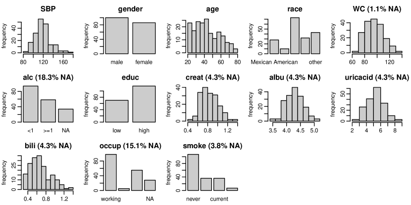
Figure 1: Distribution of the variables in the NHANES data (with percentage of missing values given for incomplete variables).

The pattern of missing values in the NHANES data is shown in Figure 2. This plot can be obtained using the function md_pattern(). Again, arguments color and border allow the user to change colours and arguments such as legend.position, print_xaxis and print_yaxis permit further customization.

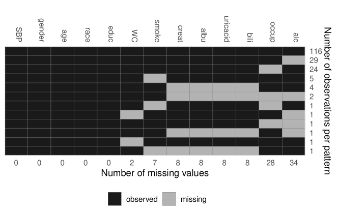
Figure 2: Missing data pattern of the NHANES data.

Each row represents a pattern of missing values, where observed (missing) values are depicted with dark (light) colour. The frequency with which each of the patterns is observed is given on the right margin, the number of missing values in each variable is given underneath the plot. Rows and columns are ordered by number of cases per pattern (decreasing) and number of missing values (increasing). The first row, for instance, shows that there are 116 complete cases, the second row that there are 29 cases for which only alc is missing. Furthermore, it is apparent that creat, albu, uricacid and bili are always missing together. Since these variables are all measured in serum, this is not surprising.

md_pattern() also returns the missing data pattern in matrix representation (pattern = TRUE), where missing and observed values are represented with a 0 and 1, respectively.

4.2 The simLong data

The simLong data is a simulated dataset mimicking a longitudinal cohort study of 200 mother-child pairs. It contains the following baseline (i.e., not time-varying) covariates

• GESTBIR: gestational age at birth in weeks; complete

• ETHN: ethnicity; binary; 2.8% missing

• AGE_M: age of the mother at intake; complete

• HEIGHT_M: height of the mother in cm; 2.0% missing

• PARITY: number of times the mother has given birth; binary; 2.4% missing

• SMOKE: smoking status of the mother during pregnancy; 3 ordered categories; 12.2% missing

• EDUC: educational level of the mother; 3 ordered categories; 7.8% missing

• MARITAL: marital status; 3 unordered categories; 7.0% missing

• ID: subject identifier

and seven longitudinal variables:

• time: measurement occasion/visit (by design, children should have been measured at/around 1, 2, 3, 4, 7, 11, 15, 20, 26, 32, 40 and 50 months of age)

• age: child’s age at measurement time in months

• hgt: child’s height in cm; 20% missing

• wgt: child’s weight in gram; 8.8% missing

• bmi: child’s BMI (body mass index) in kg/m²; 21.6% missing

• hc: child’s head circumference in cm; 23.6% missing

• sleep: child’s sleeping behaviour; 3 ordered categories; 24.7% missing

Figure 3 shows the longitudinal profiles of hgt, wgt, bmi and hc over age. All four variables clearly have a non-linear pattern over time.

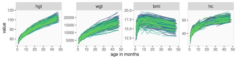
Figure 3: Trajectories of the continuous time-varying variables in the simLong data.

Histograms and bar plots of all variables in the simLong data are displayed in Figure 4. Here, the argument idvar of the function plot_all() is used to display baseline (level-2) covariates on the subject level instead of the observation level:

R> plot_all(simLong, use_level = TRUE, idvar = "ID", ncol = 5)

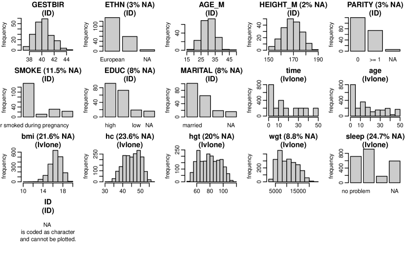
Figure 4: Distribution of the variables in the simLong data.

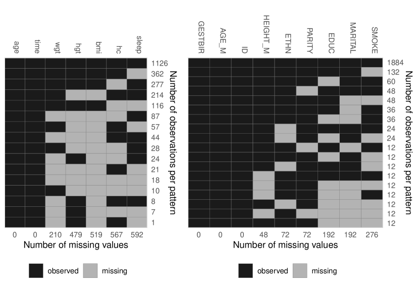
Figure 5: Missing data pattern of the simLong data (left: level-1 variables, right: level-2 variables).

The missing data pattern of the simLong data is shown in Figure 5. For readability, the pattern is given separately for the level-1 (left) and level-2 (right) variables. It is non-monotone and does not have any distinctive features.

4.3 The PBC data

For demonstration of the use of JointAI for the analysis of survival data we use the dataset PBC which is a re-coded version of the PBC data in the survival package. It contains baseline and follow-up data of 312 patients with primary biliary cirrhosis and includes the following variables:

Baseline covariates:

• id: patient identifier; complete

• futime: time until death, transplantation or censoring in days; complete

• status: event indicator (censored, transplant or dead); complete

• trt: treatment (D-penicillamine or placebo); complete

• age: patient’s age in years; complete

• sex: patient’s sex; complete

• copper: urine copper ($\mu$g/day); 0.6% missing

• trig: triglyceride (mg/dl); 9.6% missing

Time-varying covariates:

• day: number of days between enrolment and this visit date (time variable for the laboratory measurements); complete

• albumin: serum albumin (mg/dl); complete

• alk.phos: alkaline phosphatase (U/litre); 3.1% missing

• ascites: presence of ascites; 3.1% missing

• ast: aspartate aminotransferase (U/ml); complete

• bili: serum bilirubin (mg/dl); complete

• chol: serum cholesterol (mg/dl); 42.2% missing

• edema: “no”: no oedema, “(un)treated”: untreated or successfully treated 1 oedema, “edema”: oedema despite diuretic therapy; complete

• hepato: presence of hepatomegaly (enlarged liver); 3.1% missing

• platelet: platelet count; 3.8% missing

• protime: standardised blood clotting time; complete

• spiders: blood vessel malformations in the skin; 3.0% missing

• stage: histologic stage of disease (4 levels); complete

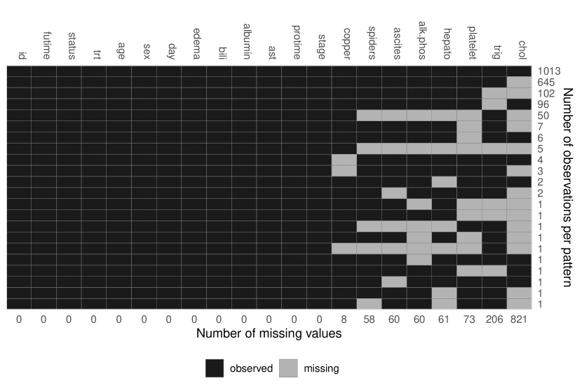
Figure 6: Missing data pattern of the PBC data.

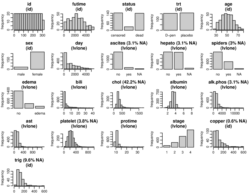
Figure 7: Distribution of the variables in the PBC data (with percentage of missing values given for incomplete variables).

The missing data pattern and distribution of the observed values of the PBC data is shown in Figures 6 and 7.

4.4 Missing data visualization and exploration

There are several R packages that provide functionality for a more in-depth exploration of incomplete data, see for example the ones listed in the CRAN task view on missing data (https://CRAN.R-project.org/view=MissingData). Particularly useful may be the packages naniar (naniar) and VIM (VIM).

5 Model specification

The main analysis functions in JointAI are lm_imp(), glm_imp(), lognorm_imp(), betareg_imp(), clm_imp(), mlogit_imp(), lme_imp(), glme_imp(), lognormmm_imp(), betamm_imp(), clmm_imp(), mlogitmm_imp(), survreg_imp(), coxph_imp() and JM_imp().

The main arguments of these functions, i.e., formula, data, family, fixed, and random, are used analogously to the specification in the standard complete data functions lm() and glm() from package stats, lme(), from package nlme (nlme) and survreg() and coxph() from package survival, for example:

R> lm_imp(formula, data, + n.chains = 3, n.adapt = 100, n.iter = 0, thin = 1, …)

R> glm_imp(formula, family, data, + n.chains = 3, n.adapt = 100, n.iter = 0, thin = 1, …)

R> lme_imp(fixed, data, random, + n.chains = 3, n.adapt = 100, n.iter = 0, thin = 1, …)

R> glme_imp(fixed, data, random, family, + n.chains = 3, n.adapt = 100, n.iter = 0, thin = 1, …)

R> survreg_imp(formula, data, + n.chains = 3, n.adapt = 100, n.iter = 0, thin = 1, …)

The specification for lognorm_imp(), betareg_imp(), and mlogit_imp() is the same as for lm_imp().

The functions lme_imp() and glme_imp() have aliases lmer_imp() and glmer_imp(), and all mixed model functions accept specification of a combined fixed and random effects formula (like in the package lme4 (lme4)) as well as the specification using fixed and random.

The arguments formula and fixed take a standard two-sided formula object, where an intercept is added automatically (except in ordinal and proportional hazards models). For the specification of random effects formulas, see Section LABEL:sec:multilevel.

clm_imp() and clmm_imp() have additional optional arguments nonprop and rev. nonprop expects a one-sided formula containing those terms of formula or fixed that should have non-proportional effects, and rev can be set to TRUE to indicate that the odds should be reversed, i.e., to model $\frac{P(y\leq k)}{P(y>k)}$ instead of $\frac{P(y>k)}{P(y\leq k)}$.

Survival models expect the left hand side of formula to be a survival object (created with the function Surv() from package survival, see Section LABEL:sec:survmod).

The argument family enables the choice of a distribution and link function from a range of options when using glm_imp() or glme_imp(). The implemented options are given in Table 1.

distribution	link
gaussian	identity, log, inverse
binomial	logit, probit, log, cloglog
Gamma	inverse, identity, log
poisson	log, identity

Table 1: Possible choices for the model family and link functions in glm_imp() and glme_imp().

For the description of the remaining arguments see below and Section LABEL:sec:MCMCSettings.

5.1 Specification of the model formula

5.1.1 Interactions

In JointAI, interactions between any type of variables (observed, incomplete, variables from different hierarchical levels) can be handled. When an incomplete variable is involved, the interaction term is re-calculated within each iteration of the MCMC sampling, using the imputed values from the current iteration. Interaction terms involving incomplete variables should, hence, not be pre-calculated as an additional variable since this would lead to inconsistent imputed values of main effect and interaction term.

Interactions between multiple variables can be specified using parentheses; for higher lever interactions the ^ operator can be used:

R> mod1a <- glm_imp(educ   gender * (age + smoke + creat), + data = NHANES, family = binomial())

R> mod1b <- glm_imp(educ   gender + (age + smoke + creat)^3, + data = NHANES, family = binomial())

5.1.2 Non-linear functional forms

In practice, associations between outcome and covariates do not always meet the standard assumption of linearity. Often, assuming a logarithmic, quadratic or other non-linear effect is more appropriate.

For completely observed covariates, JointAI can handle any common type of function implemented in R, including splines, e.g., using ns() or bs() from the package splines. Since functions involving variables that have missing values need to be re-calculated in each iteration of the MCMC sampling, currently, only functions that are available in JAGS can be used for incomplete variables. Those functions include:

• log(), exp()

• sqrt(), polynomials (using I())

• abs()

• sin(), cos()

• algebraic operations (wrapped in I()) involving one or multiple (in)complete variables, as long as the formula can be interpreted by JAGS.

The list of functions implemented in JAGS can be found in the JAGS user manual (JAGSmanual) available at https://sourceforge.net/projects/mcmc-jags/files/Manuals/.

Some examples (that do not necessarily have a meaningful interpretation or good model fit) are:

R> mod2a <- lm_imp(SBP   age + gender + abs(bili - creat), data = NHANES)

R> library("splines") R> mod2b <- lm_imp(SBP   ns(age, df = 2) + gender + I(bili^2) + I(bili^3), + data = NHANES)

R> mod2c <- lm_imp(SBP   age + gender + I(creat/albu^2), data = NHANES, + trunc = list(albu = c(1e-5, NA)))

R> mod2d <- lm_imp(SBP   bili + sin(creat) + cos(albu), data = NHANES)

It is also possible to nest a function in another function.

R> mod2e <- lm_imp(SBP   age + gender + sqrt(exp(creat)/2), data = NHANES)

5.1.3 Functions with restricted support

When a function of an incomplete variable has restricted support, e.g., $\log(x)$ is only defined for $x>0$, or, in mod2c from above I(creat/albu^2) can not be calculated for albu = 0, the model specified for that incomplete variable needs to comply with these restrictions. This can either be achieved by truncating the distribution, using the argument trunc, or by selecting a distribution that meets the restrictions.

Note that truncation should be used with care. Its intended use here is to prevent issues when theoretically a variable could take a value that would result in an invalid mathematical expression. Truncation should not be used to make symmetric distributions, like the normal distribution, fit skewed data. (vonHippel2012; Rodwell2014; Geraci2018)

Example:

When using a $\log$ transformation for the covariate uricacid, we can use the default imputation method "norm" (a normal distribution) and truncate it by specifying trunc = list(uricacid = c(<lower>, <upper>)), where <lower> and <upper> are the smallest and largest values allowed:

R> mod3a <- lm_imp(SBP   age + gender + log(uricacid) + exp(creat), + trunc = list(uricacid = c(1e-5, NA)), data = NHANES)

One-sided truncation is possible by setting the limit that is not needed to NA.

Alternatively, we may choose a model for the incomplete variable (using the argument models; for more details see Section LABEL:sec:methJSS) that only imputes positive values such as a log-normal distribution or a gamma distribution:

R> mod3b <- lm_imp(SBP   age + gender + log(uricacid) + exp(creat), + models = c(uricacid = "lognorm"), data = NHANES)

R> mod3c <- lm_imp(SBP   age + gender + log(uricacid) + exp(creat), + models = c(uricacid = "glm_gamma_inverse"), data = NHANES)

5.1.4 Functions that are not available in R

It is possible to use functions that have different names in R and JAGS, or that do exist in JAGS, but not in R, by defining a new function in R that has the name of the function in JAGS.

Example:

In JAGS the inverse logit transformation is defined in the function ilogit. In base R, there is no function ilogit, but the inverse logit is available as the distribution function of the logistic distribution plogis(). Thus, we can define the function ilogit() as

R> ilogit <- plogis

and use it in the model formula

R> mod4a <- lm_imp(SBP   age + gender + ilogit(creat), data = NHANES)

5.1.5 A note on what happens inside JointAI

When a function of a complete or incomplete variable is used in the model formula, the main effect of that variable is automatically added as an auxiliary variable (more on auxiliary variables in Section LABEL:sec:auxvars), and only the main effects are used as predictors in the imputation models.

In mod2b, for example, the spline of age is used as predictor for SBP, but in the imputation model for bili, age enters with a linear effect. This can be checked using the function list_models(), which prints a list of all sub-models used in an JointAI model. Here, we are only interested in the predictor variables, and, hence, suppress printing of information on prior distributions, regression coefficients and other parameters by setting priors, regcoef and otherpars to FALSE:

R> list_models(mod2b, priors = FALSE, regcoef = FALSE, otherpars = FALSE)

Linear model for "SBP" family: gaussian link: identity * Predictor variables: (Intercept), ns(age, df = 2)1, ns(age, df = 2)2, genderfemale, I(bili^2), I(bili^3)

Linear model for "bili" family: gaussian link: identity * Predictor variables: (Intercept), age, genderfemale

When a function of a variable is specified as auxiliary variable, this function is used in the imputation models. For example, in mod4b, waist circumference (WC) is not part of the model for SBP, and the quadratic term I(WC^2) is used in the linear predictor of the imputation model for bili:

R> mod4b <- lm_imp(SBP   age + gender + bili, auxvars =   I(WC^2), + data = NHANES) R> R> list_models(mod4b, priors = FALSE, regcoef = FALSE, otherpars = FALSE)