Pseudorapidity dependent hydrodynamic response in heavy-ion collisions

Abstract

We propose a differential hydrodynamic response relation, $V_{2}(\zeta)=\int d\xi G(\zeta-\xi)\mathcal{E}_{2}(\xi)$, to describe the formation of a pseudorapidity dependent elliptic flow in heavy-ion collisions, in response to a fluctuating three-dimensional initial density profile. By analyzing the medium expansion using event-by-event simulations of 3+1D MUSIC, with initial conditions generated via the AMPT model, the differential response relation is verified. Given the response relation, we are able to separate the two-point correlation of elliptic flow in pseudorapidity into fluid response and two-point correlation of initial eccentricity. The fluid response contains information of the speed of sound and shear viscosity of the medium. From the pseudorapidity dependent response relation, a finite radius of convergence of the hydrodynamic gradient expansion is obtained with respect to realistic fluids in heavy-ion collisions.

I Introduction

In high energy heavy-ion experiments, the fluid nature of quark-gluon plasma (QGP) has been well demonstrated through the measurements of flow harmonics in multi-particle correlations Song et al. (2017). These flow harmonics can be understood as the fluid response to the decomposed azimuthal modes associated with the initial state geometrical deformations, giving rise to a series of response relations (cf. Heinz and Snellings (2013); Yan (2018) for recent reviews). In particular, the eccentricity of the initial density profile $\mathcal{E}_{2}$, which characterizes the elliptic deformation of the QGP fireball at initial time, and elliptic flow $V_{2}$ Ollitrault (1992), which characterizes the asymmetric emission of final state particles in azimuthal angles, are linearly correlated:

$$V_{2}=G_{0}\mathcal{E}_{2}\,.$$ (1)

Both $V_{2}$ and $\mathcal{E}_{2}$ fluctuate from event to event, but this linear relation has been found valid for the mid-central collisions via event-by-event hydrodynamic simulations Qiu and Heinz (2011); Niemi et al. (2013); Noronha-Hostler et al. (2016). In Eq. (1), the response coefficient $G_{0}$ depends on the fluid properties of QGP, which is a real constant in one specified centrality class. A consistent suppression of the response coefficient has been observed when dissipative corrections in the QGP become larger.

Eq. (1) has lead to many remarkable applications in heavy-ion collisions, such as the background subtraction of chiral magnetic effects Kharzeev et al. (2008) using a selected collision geometry Koch et al. (2017); Voloshin (2010). Nevertheless, as one relation between the global azimuthal asymmetry of initial and final states, knowledge of the local structure of the QGP medium is absent. In this letter, we propose a generalization of Eq. (1) to a pseudorapidity dependent hydrodynamic response. Our generalization is partly motivated by the experimental developments in heavy-ion collisions, where pseudorapidity dependent flow harmonics have been explored Khachatryan et al. (2015); Aad et al. (2014); Adam et al. (2016). Besides, the pseudorapidity dependent hydrodynamic response is expected to play a more significant role in the beam energy scan program carried out at the Relativistic Heavy-Ion Collider Luo and Xu (2017), since at lower collision energies, approximations for the fluid dynamics along the longitudinal direction with respect to Bjorken symmetry are no longer valid in theoretical models Du and Heinz (2019).

A pseudorapidity dependent generalization of Eq. (1) reveals the local properties of the QGP medium, which is of extremely significance. First, a pseudorapidity dependent hydrodynamic response allows one to detect the fluid locally, so that the transport properties of the QGP medium can be examined differentially. One such example is the attempt to extract a temperature dependent ratio of shear viscosity over the entropy density, $\eta/s(T)$ Denicol et al. (2016). Besides, if the local gradients in pseudorapidity are accessible, the convergence behavior of the hydrodynamic gradient expansion can be analyzed in realistic QGP medium with non-trivial 3+1 dimensional expansions, which would substantially extends the recent developments with respect to systems undergoing one dimensional Bjorken expansion (cf. Heller and Spalinski (2015); Heller et al. (2013); Basar and Dunne (2015)).

II Formulation

We first present a step-by-step derivation of the generalization of Eq. (1). The only assumption we have is the fluidity of QGP, so that long wave-length (small wave-number) modes dominate.

In heavy-ion collisions, from each collision event the single-particle distribution that describes the probability of particle emission with azimuthal angle ($\phi={\rm atan}(p_{y}/p_{x})$) and pseudorapidity ($\zeta={\rm atanh}(p_{z}/|\bf p|)$) dependence can be decomposed into Fourier modes

$$P(\phi,\zeta)=\frac{1}{2\pi}\sum_{n=-\infty}^{n=+\infty}V_{n}(\zeta)e^{-in\phi}\,,$$ (2)

where the Fourier coefficient defines the complex harmonic flow $V_{n}(\zeta)\equiv v_{n}(\zeta)e^{in\Psi_{n}(\zeta)}$. It is worth mentioning that the definition of flow harmonics in Eq. (2) differs from the usual one by a factor of normalized multiplicity distribution. Given the definition in Eq. (2), the integrated flow coefficient is then $V_{n}=\int_{-\infty}^{\infty}d\zeta\;V_{n}(\zeta)\,.$ Throughout this letter, we shall focus on the second harmonic, namely, elliptic flow $V_{2}(\zeta)$, while generalizations to other flow harmonics are straightforward.

Initial eccentricity $\mathcal{E}_{2}$ is a complex quantity, which characterizes the elliptical asymmetry of the three-dimensional initial density profile $\rho(\vec{x}_{\perp},\xi)$. Note that $\xi=\rm atanh(z/t)$ is the space-time rapidity, to be distinguished from the pseudorapidity $\zeta$. In order to generalize the response relation along the longitudinal direction, we consider the definition for a $\xi$-dependent eccentricity as

$$\mathcal{E}_{2}(\xi)=-\frac{\int d^{2}\vec{x}_{\perp}\;\rho(\vec{x}_{\perp},\xi)(x+iy)^{2}}{\int d\xi d^{2}\vec{x}_{\perp}\;\rho(\vec{x}_{\perp},\xi)|x+iy|^{2}}\,,$$ (3)

so that the azimuthal deformation of the density profile at a specified space-time rapidity $\xi$ is quantified. Eq. (3) is not a unique definition that introduces dependence on space-time rapidity in eccentricity Pang et al. (2016); Franco and Luzum (2019), but Eq. (3) satisfies the condition: $\mathcal{E}_{2}=\int_{-\infty}^{\infty}d\xi\;\mathcal{E}_{2}(\xi)\,,$ and more importantly,

$$d^{m}\mathcal{E}_{2}(\xi)/d\xi^{m}\rightarrow 0,\quad{\rm when}\quad|\xi|\rightarrow\infty\,,$$ (4)

for $m=0,1,2,\ldots$, which will be found useful.

Correspondingly, we generalize the linear response relation Eq. (1) as 

$$V_{2}(\zeta)=\int d\xi\;G(\zeta-\xi)\mathcal{E}_{2}(\xi)\,,$$ (5)

where the real constant response coefficient is replaced by a response function $G(\zeta-\xi)$. This function is expected entirely determined by the fluid properties of the QGP medium, which does not fluctuate in one specified centrality class where the system multiplicity is a fixed constant. Eq. (5) is a non-local and differential response relation, relating the eccentricity at one space-time rapidity $\xi$ at initial time to the flow observed at pseudorapidity $\zeta$ through the evolution of hydrodynamic modes. Note that the form of the response function implies a boost invariant background, on top of which the apparent breaking of the boost invariant symmetry in realistic heavy-ion collisions can be accounted for as perturbations introduced by the decomposed modes in $\mathcal{E}_{2}(\xi)$.

To identify the response function, it is advantageous to work with a Fourier transformation, namely, for the elliptic flow $\tilde{V}_{2}(k)=\int_{-\infty}^{\infty}d\zeta\;V_{2}(\zeta)e^{-ik\zeta}$ and initial eccentricity $\tilde{\mathcal{E}}_{2}(k)=\int_{-\infty}^{\infty}d\xi\;\mathcal{E}_{2}(\xi)e^{-ik\xi}$. In terms of the wave-number $k$, Eq. (5) becomes,

$$\tilde{V}_{2}(k)=\tilde{G}(k)\tilde{\mathcal{E}}_{2}(k)\,.$$ (6)

In the long wave-length limit with $|k|\ll k^{*}$, corresponding to the hydrodynamic regime, one is allowed to expand the response function in series of $k$. For instance, up to the second order the expansion is

$$\tilde{G}(k)=G_{0}+ikG_{1}-k^{2}G_{2}+O(k^{3})\,,$$ (7)

which amounts to

$$V_{2}(\zeta)=G_{0}\mathcal{E}_{2}(\zeta)+G_{1}\frac{d\mathcal{E}_{2}(\zeta)}{d\zeta}+G_{2}\frac{d^{2}\mathcal{E}_{2}(\zeta)}{d\zeta^{2}}+O\left(\frac{d^{3}}{d\zeta^{3}}\right)\,,$$ (8)

in the $\zeta$-space. By construction, these expansion coefficients are real constants, to be determined later. Because of the boost-invariant background, reflection symmetry is implied so that odd order response coefficients must vanish.

Several comments are in order. First, the leading order term can be identified as the response of the global elliptic asymmetry, while higher order terms ($O(k)$ and beyond) do not contribute after an integration over pseudorapidity. Therefore, Eq. (1) will be recovered from Eq. (8) after an integration over $\zeta$. Secondly, these higher order terms in the series expansion correspond to the hydro gradients, which characterize modes satisfying a gapless dispersion relation. As is evident in the response relation, these hydrodynamic gradients are specified as derivatives in space-time rapidity, as a consequence of perturbations of the initial state density profile along $\xi$. Thirdly, validity of the hydrodynamic gradient expansion is determined by its convergence behavior. The radius of convergence $k^{*}$, for instance, is finite if the hydrodynamic gradient expansion is convergent Grozdanov et al. (2019a). If, on the other hand, the gradient expansion is asymptotic, practical applications of the response formulation would rely on a Borel resummation method Heller and Spalinski (2015). As will be clear in Appendix A, the existence of a finite $k^{*}$ results in an effective regularization of the eccentricity distribution along space-time rapidity, which smooths out local structures. More detailed discussion on the convergence behavior and $k^{*}$ will be given in Sec. III.2.

To access these expansion coefficients $G_{n}$’s, it is natural to define new sets of flow observables and initial eccentricity variables weighted with powers of $\zeta$ (or $\xi$),

$$V^{(n)}_{2}\equiv \int d\zeta\zeta^{n}V_{2}(\zeta)/n!\,,$$ (9a)

$$\mathcal{E}^{(n)}_{2}\equiv \int d\xi\xi^{n}\mathcal{E}_{2}(\xi)/n!\,.$$ (9b)

These new variables are defined according to the series expansion form Eq. (8), reflecting the nature of hydrodynamic mode evolution. Especially, $\mathcal{E}_{2}^{(n)}$ provides an alternative mode decomposition of the initial eccentricity distribution along the space-time rapidity, comparing to those developed on grounds of initial state geometrical fluctuations Bzdak and Teaney (2013); Jia et al. (2016). Using integration by parts repeatedly, the generalized linear response relation Eq. (5) can be written in an alternate form as

$$V_{2}^{(n)}=\sum_{i=0}^{n}(-1)^{i}G_{i}\mathcal{E}_{2}^{(n-i)}\,.$$ (10)

Note that Eq. (4) has been taken into account implicitly to obtain Eq. (10). Note also that the leading order relation $V_{2}^{(0)}=G_{0}\mathcal{E}_{2}^{(0)}$ is the linear response relation presented in Eq. (1), and the response coefficient can be calculated in event-by-event hydrodynamic simulations Noronha-Hostler et al. (2016): $G_{0}=\left\langle V_{2}^{(0)}\mathcal{E}_{2}^{(0)*}\right\rangle\Big{/}\left\langle\mathcal{E}_{2}^{(0)}\mathcal{E}_{2}^{(0)*}\right\rangle$, where the angular brackets indicate event average. Given the leading order response coefficient $G_{0}$, one realizes a linear response relation between $\mathcal{E}_{2}^{(0)}$ and $V_{2}^{(1)}-G_{0}\mathcal{E}_{2}^{(1)}$, with the slope identified as $G_{1}$. In a similar way, a set of linear relations can be realized between $\mathcal{E}_{2}^{(0)}$ and $V_{2}^{(n)}-\sum_{i=0}^{n-1}(-1)^{i}G_{i}\mathcal{E}_{2}^{(n-i)}$, with $G_{n}$ calculated recursively as

$$(-1)^{n}G_{n}=$$ (11)

$$\left\langle\left(V_{2}^{(n)}-\sum_{i=0}^{n-1}(-1)^{i}G_{i}\mathcal{E}_{2}^{(n-i)}\right)\mathcal{E}_{2}^{(0)*}\right\rangle\Big{/}\left\langle\mathcal{E}_{2}^{(0)}\mathcal{E}_{2}^{(0)*}\right\rangle$$ (12)

III Event-by-event hydrodynamic simulations

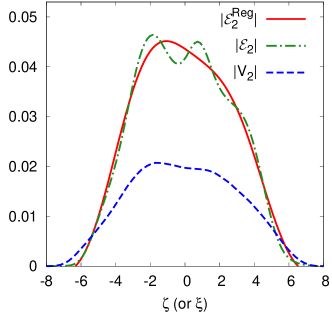
Figure 1: (Color online) Longitudinal distribution of initial eccentricity and flow in one collision event from numerical hydrodynamic simulations. The green dash-dotted line and the blue dashed lines correspond to the magnitude of eccentricity and elliptic flow, respectively. With $k^{*}=1.2$, the red solid line shows the regularization of initial eccentricity distribution due to the finite radius of convergence of the longitudinal hydrodynamic response, according to Eq. (16).

To test the analytical formulations of the longitudinal hydrodynamics response, we carry out realistic event-by-event hydrodynamic simulations, for the Pb-Pb collision system with $\sqrt{s_{NN}}=2.76$ TeV at the LHC, for events in centrality class of 30-40%. This is realized by the 3+1D MUSIC Schenke et al. (2010, 2011); Paquet et al. (2016), with respect to random 3D initial conditions generated by the AMPT model Lin et al. (2005); Lin (2014). The initial density profile is obtained in a similar strategy as in Ref. Li et al. (2017), with an overall constant factor adjusted to reconcile the mismatch of viscosity in AMPT and viscous hydrodynamics Pang et al. (2016); Chattopadhyay et al. (2018). Note that non-trivial longitudinal density distribution with fluctuations in the AMPT model have been implemented. In Fig. 1, the distribution of eccentricity magnitude along space-time rapidity in one collision event is shown as the green dash-dotted line, where bumps appear as a consequence of longitudinal fluctuations.

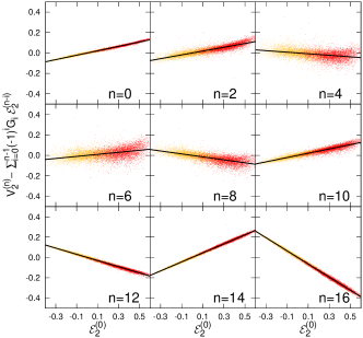
Figure 2: (Color online) Scatter plot showing the linear relations between $\mathcal{E}_{2}^{(0)}$ and $V_{2}^{(n)}-\sum_{i=0}^{n-1}(-1)^{i}G_{i}\mathcal{E}_{2}^{(n-i)}$, with coefficients $G_{n}$’s solved recursively with respect to Eq. (11) (slopes of solid lines), using event-by-event 3+1D hydro simulations with $\eta/s=0.08$. Red and yellow points are for the real and imaginary parts in the linear relation respectively. Slopes of odd orders (not shown) are consistent with zero.

MUSIC solves the second order viscous hydrodynamics with respect to a 3+1D expanding system, in which a cross-over from the QGP to hadron gas is implied in an equation of state obtained from lattice QCD. We calculate elliptic flow $V_{2}$ from thermal pions. Throughout our analyses, statistical errors from simulations are estimated using the Jackknife resampling method. In the current study, we only consider shear viscous corrections with a constant ratio of shear viscosity to the entropy density, $\eta/s$, while second order transport coefficients are fixed accordingly. More details on the numerical simulations of MUSIC, such as the equation of state, the freeze-out prescription, etc., can be found in Ref. Schenke et al. (2010, 2011); Paquet et al. (2016) and references therein.

Given the results from hydrodynamic simulations, the constant response coefficients can be calculated, as well as the linear relations between $\mathcal{E}_{2}^{(0)}$ and $V_{2}^{(n)}-\sum_{i=0}^{n-1}(-1)^{i}G_{i}\mathcal{E}_{2}^{(n-i)}$. Scatter plots in Fig. 2 present these linear relations respectively from the real part (red points) and the imaginary part (yellow points), from event-by-event hydro simulations of approximately 5000 events with a constant $\eta/s=0.08$. For even orders up to $n=16$, apparent linear relations are shown, with slopes compatible with those calculated with respect to Eq. (11).  We notice that slopes of odd orders are consistent with zero within errors, as anticipated.

III.1 Two-point correlation of $V_{2}$

The pseudorapidity dependent response relation Eq. (5) is non-local, which implies that the generation of $V_{2}$ at one pseudorapidity receives contributions from other space-time rapidities. But the response along longitudinal direction is limited by the speed of sound in fluid systems. This effect can be shown in the analysis of two-point correlations. We define

$$\left\langle(\Delta\zeta)^{2}\right\rangle\equiv\frac{\int d\zeta d\zeta^{\prime}\left\langle V_{2}(\zeta)V_{2}^{*}(\zeta^{\prime})\right\rangle(\zeta^{\prime}-\zeta)^{2}}{\int d\zeta d\zeta^{\prime}\left\langle V_{2}(\zeta)V_{2}^{*}(\zeta^{\prime})\right\rangle},$$ (14)

to characterize the length of the two-point correlation measured via elliptic flow at different pseudo-rapidities. With the response relation derived in Eq. (9) and Eq. (10), in particular, considering the fact that $G_{1}=0$, it can be proved that

$$\left\langle(\Delta\zeta)^{2}\right\rangle=\left\langle(\Delta\xi)^{2}\right\rangle+4G_{2}/G_{0}\,.$$ (15)

The length of the initial state eccentricity two-point correlation $\left\langle(\Delta\xi)^{2}\right\rangle$ is defined according to Eq. (14) through $\mathcal{E}_{2}(\xi)$. Eq. (15) states that the increase of the two-point correlation length in elliptic flow comparing to that in the initial eccentricity is purely an effect of fluid dynamics. This can be understood as a direct consequence of sound propagation, reflected in the ratio $G_{2}/G_{0}$, that initial perturbations propagate in speed of sound $c_{s}$ along the longitudinal direction Kapusta et al. (2012). Since sound propagation is damped as a result of fluid dissipations: Shear, bulk, etc., in dissipative fluids the two-point correlation at the final stage is reduced.

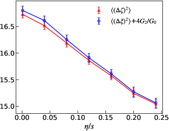
Figure 3: (Color online) Two-point correlation length of $V_{2}$ and the expectations from Eq. (15), as a function of $\eta/s$, for the Pb-Pb system of $\sqrt{s_{NN}}=2.76$ TeV in centrality class 30-40%, where the initial two-point correlation length is $\left\langle(\Delta\xi)^{2}\right\rangle=12.81\pm 0.08$.

Fig. 3 shows the numerical results of about 1000 events from hydrodynamic simulations with different values of $\eta/s$. The obtained length of the two-point correlation of $V_{2}$ is plotted as a function of $\eta/s$, which agrees with expectation from Eq. (15) within statistical errors. When $\eta/s\to 0$, the length of two-point correlation approaches an upper bound determined by the sound horizon of QGP medium. Reduction of the correlation length, or the ratio $G_{2}/G_{0}$, due to shear viscous correction is clear and systematic. Subject to boundary corrections due to the experimental acceptance along pseudorapidity, $\left\langle(\Delta\zeta)^{2}\right\rangle$ is a measurable in heavy-ion experiments, providing a novel probe of $\eta/s$ in the QGP medium.

III.2 The radius of convergence

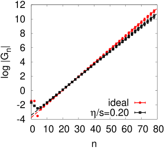
Figure 4: (Color online) Exponential increase of the expansion coefficients $|G_{n}|$ with respect to $n$. Lines are linear fit with slope 0.190 (ideal) and 0.176 ($\eta/s=0.2$).

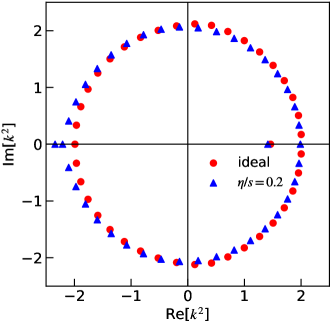
Figure 5: (Color online) Pole structure in the complex $k^{2}$-plane from a Padé approximation of the gradient expansion. The pole closest to origin is on the positive real axis: $(1.4615,0)$ for the ideal case and $(1.4126,0)$ for the case of $\eta/s=0.2$.

With the expansion coefficients calculated from event-by-event hydrodynamic simulations, we are able to explore the convergence behavior of the hydrodynamic gradient expansion in Eq. (7). Especially, the gradient expansion corresponds to the fluid properties in a realistic, 3+1D expanding QGP medium obeying lattice equation of state.

Owing to the reflection symmetry, we ignore contributions from odd orders of the expansion. For $n>2$, we notice that the sign of $G_{n}$ of even orders flips. In Fig. 4, the calculated even order coefficients are shown, from hydrodynamic simulations of roughly 1000 events, using $\eta/s=0.001$ (ideal) and $\eta/s=0.2$, respectively. For $n>4$, these $G_{n}$’s grow exponentially: $\log|G_{n}|\propto\alpha n$, which implies a finite radius of convergence. Therefore, the hydrodynamic gradient expansion in this current case is convergent. The slope in Fig. 4 determines the radius of convergence. Alternatively, one may also apply a diagonal Padé approximation for the gradient expansion. Convergence behavior can thus be revealed from the singularity structure of the Padé approximation. The resulted poles in the complex $k^{2}$-plane are shown in Fig. 5. When $n>70$, the singularity structure of the Padé approximation stabilizes. In particular, in addition to those poles lying around a circle, there exists one pole closest to the origin on the positive real axis, which determines the radius of convergence.

From both ways, the obtained radii of convergence are finite. Numerical values of the radii are consistent, which we identify as the upper bound of the gradient expansion $k^{*}$. From ideal hydrodynamic simulations, we find $k^{*}=1.209$ (slope) and $1.209$ (Padé), while for the case of $\eta/s=0.2$ we find $k^{*}=1.192$ (slope) and $1.189$ (Padé). When shear viscosity decreases, there seems to be a trend that $k^{*}$ grows Grozdanov et al. (2019a, b). However, due to the effect of expansion, we find that $k^{*}$ saturates to a constant in an ideal fluid even though the mean free path approaches zero.

For a medium system away from local equilibrium, it is known that the gradient expansion consisting of higher order dissipative corrections is asymptotic Heller and Spalinski (2015); Heller et al. (2013); Basar and Dunne (2015). Origin of such divergence can be intuitively attribute to the fact that the number of higher order viscous terms has a factorial increase. However, it is different in the current case concerning perturbations on top of the medium system in or close to local equilibrium, where gradients are taken into account with respect to the dispersion relation Withers (2018); Grozdanov et al. (2019a, b).

In the current study, the existence of a finite radius of convergence of the gradient expansion has an important physical interpretation. The upper bound $k^{*}$ of the expansion implies a length scale limit in the space-time rapidity of the initial eccentricity profile $\mathcal{E}_{2}(\xi)$. This is the scale that determines the resolution of fluid response to initial state local structures. Although for a static medium this effect can be generically understood as the fact that the fluid behavior of a medium system must be visible at a scale greater than the mean free path and one expects $k^{*}\sim 1/l_{\rm mfp}$, in the medium with non-trivial 3+1D expansion it becomes more complicated. As a consequence of the hydro response and finite $k^{*}$, a regularization scheme for the initial eccentricity profile can be introduced, leading to a regularized eccentricity profile $\mathcal{E}_{2}^{\rm Reg}(\xi)$. Derivation of the regularization scheme is given in Appendix A. In Fig. 1, one finds in the resulted $\mathcal{E}_{2}^{\rm Reg}$ the local perturbations are smoothed out, giving rise to a consistent shape comparing with the distribution of flow where bumpy structures are merely seen.

IV Summary and discussions

We have derived the generalized formulation of pseudorapidity dependent hydrodynamic response. The generalized form is a non-local relation that interprets the formation of elliptic flow at different pseudo-rapdities as a consequence of longitudinal fluid response, which provides a novel picture of longitudinal flow generation that differs from some previous studies (cf. Ref. Bożek et al. (2015); Sakai et al. (2019)). The formulation is applicable to other flow harmonics as well, when complexities involving nonlinearities do not arise Noronha-Hostler et al. (2016); Teaney and Yan (2012).

The longitudinal fluid response can be quantified by a set of constant coefficients $G_{n}$’s, and a new set of flow observables in Eq. (9). This is the main result of this letter, which has been shown valid through realistic event-by-event hydrodynamic simulations for a 3+1D expanding system in heavy-ion collisions. The second order expansion coefficient $G_{2}$ is found to be sensitive to the sound mode propagation, contributing to the increase of two-point correlation length of the elliptic flow. Shear viscous correction in the fluid reduces two-point correlation, as expected from the damping of sound. Therefore, two-point correlation of flow provides a new measurable to investigate the shear viscosity of the QGP medium in experiments.

Within the formulation of pseudorapidity dependent hydrodynamic response, the expansion coefficients $G_{n}$’s can be calculated with respect to a realistic expanding QGP medium. Given these expansion coefficients, hydrodynamic gradient expansion can be analyzed. In this current study, we solved 3+1D MUSIC with respect to fluctuating initial conditions, which represents the fluid response to perturbations on top of a fluid medium that obeys second order viscous hydrodynamics. Generation of the elliptic flow from gradients along the longitudinal direction thus reflects the evolution of sound and shear diffusive modes, as in the hydrodynamic dispersion relations. A finite radius of convergence is observed, which confirms the finding that hydrodynamic gradient expansion associated with the dispersion relation is convergent Withers (2018); Grozdanov et al. (2019a, b).

Acknowledgements – We thank Subikash Choudhury for his contributions at an early stage of this project. We thank Xiao-Liang Xia for his help in generating the hydrodynamic initial conditions. We thank Huan Zhong Huang for carefully reading the manuscript and for his very inspiring comments. We thank Jean-Yves Ollitrault for pointing out the fact that odd order expansion coefficients must vanish with respect to the boost invariant background. This work is supported by National Natural Science Foundation of China (NSFC) under Grant No. 11975079 and the China Postdoctoral Science Foundation under Grant No. 2019M661333 (HL).

Appendix A Regularization of the eccentricity distribution with finite $k^{*}$

The existence of a finite radius of convergence $k^{*}$ in the hydrodynamic gradient expansion effectively introduces regularization of the initial state eccentricity distribution. This effect can be formulated through corrections to the original Fourier transform of the eccentricity distribution,

$$\mathcal{E}_{2}^{\rm Reg}(\xi)= \int_{-k^{*}}^{k^{*}}\frac{dk}{2\pi}e^{ik\xi}\tilde{\mathcal{E}}_{2}(k)=\int_{-k^{*}}^{k^{*}}\frac{dk}{2\pi}e^{ik\xi}\int_{-\infty}^{\infty}d\xi^{\prime}\mathcal{E}_{2}(\xi^{\prime})e^{-ik\xi^{\prime}}$$ (16)

$$= \int_{-\infty}^{\infty}d\xi^{\prime}\mathcal{E}_{2}(\xi^{\prime})R(\xi-\xi^{\prime};k^{*})\,,$$ (17)

where accordingly a regularization function is defined,

$$R(\xi-\xi^{\prime};k^{*})\equiv\frac{\sin(k^{*}(\xi-\xi^{\prime}))}{\pi(\xi-\xi^{\prime})}=\int_{-k^{*}}^{k^{*}}\frac{dk}{2\pi}\;e^{ik(\xi-\xi^{\prime})}\,.$$ (18)

Apparently, for $k^{*}\to\infty$, the function reduces to a Dirac delta function: $R(\xi-\xi^{\prime};k^{*})\to\delta(\xi-\xi^{\prime})$. In the opposite limit: $k^{*}\to 0$, one finds that

$$\frac{d}{d\xi}R(\xi-\xi^{\prime};k^{*})\to 0\,,$$ (19)

which gives rise to a boost invariant $\mathcal{E}_{2}^{\rm Reg}(\xi)$.

References

- Song et al. (2017) Huichao Song, You Zhou, and Katarina Gajdosova, “Collective flow and hydrodynamics in large and small systems at the LHC,” Nucl. Sci. Tech. 28, 99 (2017), arXiv:1703.00670 [nucl-th] .
- Heinz and Snellings (2013) Ulrich Heinz and Raimond Snellings, “Collective flow and viscosity in relativistic heavy-ion collisions,” Ann. Rev. Nucl. Part. Sci. 63, 123–151 (2013), arXiv:1301.2826 [nucl-th] .
- Yan (2018) Li Yan, “A flow paradigm in heavy-ion collisions,” Chin. Phys. C42, 042001 (2018), arXiv:1712.04580 [nucl-th] .
- Ollitrault (1992) Jean-Yves Ollitrault, “Anisotropy as a signature of transverse collective flow,” Phys. Rev. D46, 229–245 (1992).
- Qiu and Heinz (2011) Zhi Qiu and Ulrich W. Heinz, “Event-by-event shape and flow fluctuations of relativistic heavy-ion collision fireballs,” Phys. Rev. C84, 024911 (2011), arXiv:1104.0650 [nucl-th] .
- Niemi et al. (2013) H. Niemi, G. S. Denicol, H. Holopainen, and P. Huovinen, “Event-by-event distributions of azimuthal asymmetries in ultrarelativistic heavy-ion collisions,” Phys. Rev. C87, 054901 (2013), arXiv:1212.1008 [nucl-th] .
- Noronha-Hostler et al. (2016) Jacquelyn Noronha-Hostler, Li Yan, Fernando G. Gardim, and Jean-Yves Ollitrault, “Linear and cubic response to the initial eccentricity in heavy-ion collisions,” Phys. Rev. C93, 014909 (2016), arXiv:1511.03896 [nucl-th] .
- Kharzeev et al. (2008) Dmitri E. Kharzeev, Larry D. McLerran, and Harmen J. Warringa, “The Effects of topological charge change in heavy ion collisions: ’Event by event P and CP violation’,” Nucl. Phys. A803, 227–253 (2008), arXiv:0711.0950 [hep-ph] .
- Koch et al. (2017) Volker Koch, Soeren Schlichting, Vladimir Skokov, Paul Sorensen, Jim Thomas, Sergei Voloshin, Gang Wang, and Ho-Ung Yee, “Status of the chiral magnetic effect and collisions of isobars,” Chin. Phys. C41, 072001 (2017), arXiv:1608.00982 [nucl-th] .
- Voloshin (2010) Sergei A. Voloshin, “Testing the Chiral Magnetic Effect with Central U+U collisions,” Phys. Rev. Lett. 105, 172301 (2010), arXiv:1006.1020 [nucl-th] .
- Khachatryan et al. (2015) Vardan Khachatryan et al. (CMS), “Evidence for transverse momentum and pseudorapidity dependent event plane fluctuations in PbPb and pPb collisions,” Phys. Rev. C92, 034911 (2015), arXiv:1503.01692 [nucl-ex] .
- Aad et al. (2014) Georges Aad et al. (ATLAS), “Measurement of the centrality and pseudorapidity dependence of the integrated elliptic flow in lead-lead collisions at TeV with the ATLAS detector,” Eur. Phys. J. C74, 2982 (2014), arXiv:1405.3936 [hep-ex] .
- Adam et al. (2016) Jaroslav Adam et al. (ALICE), “Pseudorapidity dependence of the anisotropic flow of charged particles in Pb-Pb collisions at TeV,” Phys. Lett. B762, 376–388 (2016), arXiv:1605.02035 [nucl-ex] .
- Luo and Xu (2017) Xiaofeng Luo and Nu Xu, “Search for the QCD Critical Point with Fluctuations of Conserved Quantities in Relativistic Heavy-Ion Collisions at RHIC : An Overview,” Nucl. Sci. Tech. 28, 112 (2017), arXiv:1701.02105 [nucl-ex] .
- Du and Heinz (2019) Lipei Du and Ulrich Heinz, “(3+1)-dimensional dissipative relativistic fluid dynamics at non-zero net baryon density,” (2019), 10.1016/j.cpc.2019.107090, arXiv:1906.11181 [nucl-th] .
- Denicol et al. (2016) Gabriel Denicol, Akihiko Monnai, and Bjoern Schenke, “Moving forward to constrain the shear viscosity of QCD matter,” Phys. Rev. Lett. 116, 212301 (2016), arXiv:1512.01538 [nucl-th] .
- Heller and Spalinski (2015) Michal P. Heller and Michal Spalinski, “Hydrodynamics Beyond the Gradient Expansion: Resurgence and Resummation,” Phys. Rev. Lett. 115, 072501 (2015), arXiv:1503.07514 [hep-th] .
- Heller et al. (2013) Michal P. Heller, Romuald A. Janik, and Przemyslaw Witaszczyk, “Hydrodynamic Gradient Expansion in Gauge Theory Plasmas,” Phys. Rev. Lett. 110, 211602 (2013), arXiv:1302.0697 [hep-th] .
- Basar and Dunne (2015) Gokce Basar and Gerald V. Dunne, “Hydrodynamics, resurgence, and transasymptotics,” Phys. Rev. D92, 125011 (2015), arXiv:1509.05046 [hep-th] .
- Pang et al. (2016) Long-Gang Pang, Hannah Petersen, Guang-You Qin, Victor Roy, and Xin-Nian Wang, “Decorrelation of anisotropic flow along the longitudinal direction,” Eur. Phys. J. A52, 97 (2016), arXiv:1511.04131 [nucl-th] .
- Franco and Luzum (2019) Rodrigo Franco and Matthew Luzum, “Rapidity-dependent eccentricity scaling in relativistic heavy-ion collisions,” (2019), arXiv:1910.14598 [nucl-th] .
- Grozdanov et al. (2019a) Sašo Grozdanov, Pavel K. Kovtun, Andrei O. Starinets, and Petar Tadić, “Convergence of the Gradient Expansion in Hydrodynamics,” Phys. Rev. Lett. 122, 251601 (2019a), arXiv:1904.01018 [hep-th] .
- Bzdak and Teaney (2013) Adam Bzdak and Derek Teaney, “Longitudinal fluctuations of the fireball density in heavy-ion collisions,” Phys. Rev. C87, 024906 (2013), arXiv:1210.1965 [nucl-th] .
- Jia et al. (2016) Jiangyong Jia, Sooraj Radhakrishnan, and Mingliang Zhou, “Forward-backward multiplicity fluctuation and longitudinal harmonics in high-energy nuclear collisions,” Phys. Rev. C93, 044905 (2016), arXiv:1506.03496 [nucl-th] .
- Schenke et al. (2010) Bjoern Schenke, Sangyong Jeon, and Charles Gale, “(3+1)D hydrodynamic simulation of relativistic heavy-ion collisions,” Phys. Rev. C82, 014903 (2010), arXiv:1004.1408 [hep-ph] .
- Schenke et al. (2011) Bjorn Schenke, Sangyong Jeon, and Charles Gale, “Elliptic and triangular flow in event-by-event (3+1)D viscous hydrodynamics,” Phys. Rev. Lett. 106, 042301 (2011), arXiv:1009.3244 [hep-ph] .
- Paquet et al. (2016) Jean-François Paquet, Chun Shen, Gabriel S. Denicol, Matthew Luzum, Björn Schenke, Sangyong Jeon, and Charles Gale, “Production of photons in relativistic heavy-ion collisions,” Phys. Rev. C93, 044906 (2016), arXiv:1509.06738 [hep-ph] .
- Lin et al. (2005) Zi-Wei Lin, Che Ming Ko, Bao-An Li, Bin Zhang, and Subrata Pal, “A Multi-phase transport model for relativistic heavy ion collisions,” Phys. Rev. C72, 064901 (2005), arXiv:nucl-th/0411110 [nucl-th] .
- Lin (2014) Zi-Wei Lin, “Evolution of transverse flow and effective temperatures in the parton phase from a multi-phase transport model,” Phys. Rev. C90, 014904 (2014), arXiv:1403.6321 [nucl-th] .
- Li et al. (2017) Hui Li, Long-Gang Pang, Qun Wang, and Xiao-Liang Xia, “Global polarization in heavy-ion collisions from a transport model,” Phys. Rev. C96, 054908 (2017), arXiv:1704.01507 [nucl-th] .
- Chattopadhyay et al. (2018) Chandrodoy Chattopadhyay, Rajeev S. Bhalerao, Jean-Yves Ollitrault, and Subrata Pal, “Effects of initial-state dynamics on collective flow within a coupled transport and viscous hydrodynamic approach,” Phys. Rev. C97, 034915 (2018), arXiv:1710.03050 [nucl-th] .
- Kapusta et al. (2012) J. I. Kapusta, B. Muller, and M. Stephanov, “Relativistic Theory of Hydrodynamic Fluctuations with Applications to Heavy Ion Collisions,” Phys. Rev. C85, 054906 (2012), arXiv:1112.6405 [nucl-th] .
- Grozdanov et al. (2019b) Sašo Grozdanov, Pavel K. Kovtun, Andrei O. Starinets, and Petar Tadić, “The complex life of hydrodynamic modes,” JHEP 11, 097 (2019b), arXiv:1904.12862 [hep-th] .
- Withers (2018) Benjamin Withers, “Short-lived modes from hydrodynamic dispersion relations,” JHEP 06, 059 (2018), arXiv:1803.08058 [hep-th] .
- Bożek et al. (2015) Piotr Bożek, Wojciech Broniowski, and Adam Olszewski, “Hydrodynamic modeling of pseudorapidity flow correlations in relativistic heavy-ion collisions and the torque effect,” Phys. Rev. C91, 054912 (2015), arXiv:1503.07425 [nucl-th] .
- Sakai et al. (2019) Azumi Sakai, Koichi Murase, and Tetsufumi Hirano, “Rapidity decorrelation from hydrodynamic fluctuations,” Proceedings, 27th International Conference on Ultrarelativistic Nucleus-Nucleus Collisions (Quark Matter 2018): Venice, Italy, May 14-19, 2018, Nucl. Phys. A982, 339–342 (2019), arXiv:1807.06254 [nucl-th] .
- Teaney and Yan (2012) Derek Teaney and Li Yan, “Non linearities in the harmonic spectrum of heavy ion collisions with ideal and viscous hydrodynamics,” Phys. Rev. C86, 044908 (2012), arXiv:1206.1905 [nucl-th] .