Uniform Decoherence Effect on Localizable Entanglement in Random Multi-qubit Pure States

Abstract

We investigate the patterns in distributions of localizable entanglement over a pair of qubits for random multi-qubit pure states. We observe that the mean of localizable entanglement increases gradually with increasing the number of qubits of random pure states while the standard deviation of the distribution decreases. The effects on the distributions, when the random pure multi-qubit states are subjected to local as well as global noisy channels, are also investigated. Unlike the noiseless scenario, the average value of the localizable entanglement remains almost constant with the increase in the number of parties for a fixed value of noise parameter. We also find out that the maximum strength of noise under which entanglement survives can be independent of the localizable entanglement content of the initial random pure states.

I Introduction

Multipartite entanglement Horodecki et al. (2009) – one of the most important traits of composite quantum systems – has been proven to be an useful ingredient in quantum protocols like quantum teleportation Bennett et al. (1993); *bouwmeester1997; *murao1999; *grudka2004; *sende2010a, quantum dense coding Bennett and Wiesner (1992); *mattle1996; *sende2010; *bruss2004; *bruss2006; *horodecki2012; *shadman2012; *das2014; *das2015, quantum cryptography Ekert (1991); *jennewein2000; *gisin2002; *pirandola2019; *hillery1999; *cleve1999; *karlsson1999, and measurement-based quantum computation Raussendorf and Briegel (2001); *hein2004; *hein2006; *briegel2009. It also reveals interesting features in quantum many-body systems Amico et al. (2008); *chiara2018, e.g., in quantum critical regions of the phase diagrams Orús (2008a) such as spin chains Wei et al. (2005); *orus2010; *biswas2014, in valence-bond solid states Orús (2008b); *dhar2013, and in topological systems Pezzè et al. (2017). This has motivated outstanding experimental advancements in creating multi-party entangled states in the laboratory using different substrates, such as atoms *mandel2003; Leibfried et al. (2005), ions Monz et al. (2011); *friis2018, photons Prevedel et al. (2009); *gao2010; *yao2012; *wang2018, superconducting qubits Barends et al. (2014); *gong2019, nuclear magnetic resonance molecules Negrevergne et al. (2006), and very recently solid state systems Bradley et al. (2019). It has been shown that with increasing number of parties in the composite quantum systems, random pure states Bengtsson and Życzkowski (2006) tend to be highly multi-party entangled Hayden et al. (2006); *kendon2002; *enriquez2018; *klobus2019, when entanglement is quantified via distance-based measures Horodecki et al. (2009); Shimony (1995); *barnum2001; *wei2003. While potential use of multipartite entanglement as resource in quantum protocols highlights the usefulness of this feature, it was shown that highly entangled random multi-party pure states may not be beneficial for computational speed-up Gross et al. (2009); *bremner2009 (cf. Richard and Noah (2003)).

A major roadblock towards the study of the characteristics and utility of multi-party entangled quantum states with higher number of parties is the limited availability of computable entanglement measures, both in pure as well as in mixed states describing arbitrarily large composite quantum systems Horodecki et al. (2009). This has motivated the search for quantum correlation measures that, on one hand, are computable for random multi-party quantum states, and on the other hand, exhibit properties similar to multi-party entanglement when the system-size is increased. Monogamy-based quantum correlations Coffman et al. (2000); Dhar et al. (2017), with measures belonging to both entanglement-separability Horodecki et al. (2009) and information-theoretic Modi et al. (2012); *bera2017 paradigms, have recently been shown to exhibit properties similar to multi-party entanglement for random multi-party pure states Rethinasamy et al. (2019).

In this paper, we focus on the entanglement concentrated over chosen subsystem(s) of the multi-party random quantum states via local independent projective measurements on the rest of the system, which is referred to as localizable entanglement (LE) Verstraete et al. (2004a); *verstraete2004a; *popp2005; *jin2004 (cf. entanglement of assistance DiVincenzo et al. (1998); *smolin2005 and assisted mutual information Streltsov et al. (2015)). Such quantification and characterization of entanglement has been shown to be appropriate and advantageous in graph states used in measurement-based quantum computation Hein et al. (2004); *hein2006, in stabilizer states with and without noise Amaro et al. (2018); *amaro2019, in defining correlation lengths in quantum many-body systems Verstraete et al. (2004a); *verstraete2004a; *popp2005; *jin2004, and in protocols like entanglement percolation in quantum networks Acín et al. (2007). The concept of localizable entanglement has recently been generalized for concentrating entanglement over multipartite subsystems Sadhukhan et al. (2017). It was argued that for a tripartite state, localizable entanglement is not a tripartite entanglement monotone and can also not be considered as a bipartite measure Gour and Spekkens (2006). Therefore, the behavior of localizable entanglement for random pure states can not be inferred from the previous results based on multi-party distance-based and monogamy-based entanglement measures.

Towards this aim, we ask the following question: Do most of the multi-party random pure states also possess high values of localizable entanglement computed over a chosen bipartite subsystem? We answer this query affirmatively. Specifically, we Haar uniformly generate three-, four-, and five-qubit random pure states and determine the LE in terms of entanglement of formation Wootters (1998, 2001) over two of the qubits obtained via optimizing local projection measurement(s) on the rest. We observe that the values of localizable entanglement follow specific frequency distributions. To quantify the pattern, we determine different metrics of these distributions, such as mean, standard deviation, and skewness, in order to understand how LE over a qubit-pair behaves on average when the number of qubits in the system is increased. Our investigation indicates that the mean of LE over a qubit-pair in the case of multi-qubit systems increases gradually with increasing the number of qubits. On the other hand, the standard deviation of the distribution of LE decreases when one increases the number of qubits from three to five.

To our knowledge, most of the studies on the properties of random states is limited to pure states. In this paper, we go beyond the pure states by performing a systematic study of localizable entanglement when the initial random pure state is affected by local as well as global noise, and ask the question as to how the distribution of LE changes in presence of noise. This is a reasonable query in a laboratory set-up where creation of multi-party entangled states are always affected by certain decoherence. We show that the increasing trend in the average value of localizable entanglement for random states does not alter with the variation of qubits in presence of noise. From this perspective, we also study the robustness of LE against different types of local and global noise considered in this paper. In particular, we evaluate the critical value of the strength of noise after which the localizable entanglement vanishes for a given randomly generated state and find that the amplitude damping noise destroys LE less than any other noisy channels for a fixed value of noise strength.

We organize the rest of the paper as follows. In Sec. II, we provide brief descriptions of localizable entanglement and the different models for noise considered in this paper. In Sec. III.1, the frequency distribution of the values of localizable entanglement in the case of Haar uniformly generated three-, four-, and five-qubit random pure states is discussed, and the corresponding frequency distribution metrics are calculated. Sec. III.2 describes the effect of local and global noise on these frequency distributions. The robustness of localizable entanglement against different types of noise along with a comparative study of different noise models from this viewpoint is presented in Sec. IV. The concluding remarks are in Sec. V.

II Necessary Ingredients

In this section, we first give the definition of localizable entanglement for arbitrary multi-qubit states. We also ponder on the different types of noises considered in this paper, and set the corresponding terminologies. We shall only deal with qubit systems in this paper, and the definitions as well as terminologies are tailored accordingly.

II.1 Localizable entanglement

In a multi-qubit system constituted of $n$ qubits, the maximum possible average entanglement that can be accumulated over a qubit pair by measuring independent local projection opeators on the rest of the $n-2$ qubits is called the localizable entanglement  Verstraete et al. (2004a); Popp et al. (2005); Sadhukhan et al. (2017) over the pair of qubits. In this paper, we restrict ourselves to rank-$1$ projection measurements. Without any loss in generality, we denote the qubits in the $n$-qubit system by $1,2,\cdots,n$, among which the local projection measurements are performed over the $n-2$ qubits except the first two. For a quantum state $\rho_{n}$ describing an $n$-qubit system, the LE over the qubits $1$ and $2$ is given by

$$E_{12}(\rho_{n})=\max\sum_{k=1}^{2^{n-2}}p_{k}\mathcal{E}(\varrho_{12}^{(k)}).$$ (1)

Here, the multi-index $k\equiv{k_{3}^{\prime}k_{4}^{\prime}\cdots k_{n}^{\prime}}$ denotes the outcome of the rank-$1$ projection measurements corresponding to the projector $P_{i}^{(k_{i}^{\prime})}$ on the qubit $i=3,\cdots,n$, and $\mathcal{E}$ denotes a pre-decided bipartite entanglement measure, also known as the seed measure Sadhukhan et al. (2017), which is computed on the reduced post-measured state $\varrho_{12}^{(k)}$ of the qubit-pair, $(1,2)$. For two-qubit states, computable entanglement measures include entanglement of formation Wootters (1998), which we will compute in this paper, and logarithmic negativity Vidal and Werner (2002). The state $\varrho_{12}^{(k)}$ reads as

$$\varrho_{12}^{(k)}=\text{Tr}_{3,4,\cdots,n}\left[\rho_{n}^{(k)}\right],$$ (2)

where $\rho_{n}^{(k)}$ is the post-measurement $n$-qubit state corresponding to the outcome $k$, given by

$$\rho_{n}^{(k)}=\frac{1}{p_{k}}\mathcal{M}_{k}\rho_{n}\mathcal{M}_{k}^{\dagger}.$$ (3)

The probability of obtaining the measurement outcome $k$ is $p_{k}=\text{Tr}\left[\mathcal{M}_{k}\rho_{n}\mathcal{M}_{k}^{\dagger}\right]$, where

$$\mathcal{M}_{k}=I_{1}\otimes I_{2}\otimes\left[\bigotimes_{i=3}^{n}P_{i}^{(k_{i}^{\prime})}\right],$$ (4)

with $I_{1}$ and $I_{2}$ being the identity operator in the Hilbert space of qubits $1$ and $2$. The maximization in Eq. (1) is performed over a complete set of local rank-$1$ projection measurements on the $n-2$ qubits, which, in general, is difficult to perform. In the case of qubit systems, the rank-$1$ projectors on a qubit $i$ can be parametrized in terms of two real parameters $(\theta_{i},\phi_{i})$ as $P_{i}^{(k_{i}^{\prime})}=\ket{k_{i}^{\prime}}\bra{k_{i}^{\prime}}$, $k_{i}^{\prime}=a,b$, with Nielsen and Chuang (2010)

$$\ket{a}_{i} = \cos\frac{\theta_{i}}{2}\ket{0}_{i}+\text{e}^{\text{i}\phi_{i}}\sin\frac{\theta_{i}}{2}\ket{1}_{i},$$

$$\ket{b}_{i} = \sin\frac{\theta_{i}}{2}\ket{0}_{i}-\text{e}^{\text{i}\phi_{i}}\cos\frac{\theta_{i}}{2}\ket{1}_{i},$$ (5)

where $0\leq\theta_{i}<\pi$, $0\leq\phi_{i}\leq 2\pi$, $\{\ket{0}_{i},\ket{1}_{i}\}$ being the computational basis of the Hilbert space of qubit $i$.

To answer the questions raised in this paper, one needs to compute the exact value of LE corresponding to arbitrary multi-qubit quantum states, pure or mixed, with high number of qubits via performing the maximization involved in the definition of LE (Eq. (1)). Although the parametrization in Eq. (5) reduces the maximization to a $2(n-2)$ parameter optimization problem for an arbitrary $n$-qubit quantum state, obtaining the optimal basis for computing the exact value of LE can still be a challenging task when $2(n-2)$ is a large integer. This is due to the fact that the optimization depends explicitly on the localizable entanglement function, which in turn depends on the seed measure $\mathcal{E}$. Except two-qubit states, exact computation of an entanglement measure for an arbitrary mixed quantum state is usually difficult Horodecki et al. (2009). Besides, the determination of localizable entanglement also includes applications of the measurement operators $\mathcal{M}_{k}$ corresponding to each measurement outcome, which has a dimensionality exponential in $n$, given by $2^{n-2}$. Also, reduction of the post-measured states, obtained via partial trace over $2^{n-2}$ dimensions is, in general, difficult, especially in noisy situations, where one has to deal with density matrices corresponding to mixed quantum states. Due to these difficulties, exact values of localizable entanglement, and the corresponding optimal bases are known only in a handful of cases involving large number of qubits Verstraete et al. (2004a); Popp et al. (2005); Sadhukhan et al. (2017); Venuti and Roncaglia (2005); Amaro et al. (2018); *amaro2019, where certain properties of the quantum states under consideration are exploited. The present problem demands computation of the exact values of localizable entanglement over a pair of qubits in arbitrary $n$-qubit systems, for which analytical solution does not exist, and one has to consider numerical recipes. In this paper, we consider upto five-qubit states, each of which correspond to a maximization of LE over $6$ real parameters. Considering the different challenges towards the exact computation of localizable entanglement, this is the maximum number of real parameters that can be handled with satisfactory numerical accuracy in our computational setup.

Note that the value and ease of computation of localizable entanglement depends also on the choice and computability of the seed measure $\mathcal{E}$ over the reduced state $\varrho_{12}^{(k)}$ of two qubits. In the situations where noise is applied to the system, one has to deal with a mixed state describing the $n$-qubit system, and the subsequent post-measured states $\varrho^{(k)}$ and reduced post-measured states $\varrho_{12}^{(k)}$ will also be mixed. For the purpose of this paper, we consider entanglement of formation (EoF) Wootters (1998); *wootters2001 as the chosen seed measure, which, for a generic two-qubit state $\varrho_{12}$, is defined as

EoF $$= -\frac{1+\sqrt{1-C^{2}}}{2}\log_{2}\left[\frac{1+\sqrt{1-C^{2}}}{2}\right]$$ (6)

$$-\frac{1-\sqrt{1-C^{2}}}{2}\log_{2}\left[\frac{1-\sqrt{1-C^{2}}}{2}\right].$$

Here, the concurrence, $C$, of the two-qubit system is given by

$$C=\max\left[0,\lambda_{1}-\lambda_{2}-\lambda_{3}-\lambda_{4}\right],$$ (7)

with $\lambda_{i}$s $(\lambda_{1}\geq\lambda_{2}\geq\lambda_{3}\geq\lambda_{4})$ being the eigenvalues of the Hermitian matrix $\varrho^{\prime}_{12}=\sqrt{\sqrt{\varrho_{12}}\tilde{\varrho}_{12}\sqrt{\varrho_{12}}}$, with $\tilde{\varrho}_{12}=\left(\sigma^{y}_{1}\otimes\sigma^{y}_{2}\right)\varrho_{12}^{\star}\left(\sigma^{y}_{1}\otimes\sigma^{y}_{2}\right)$.

II.2 Noise Models

To analyze the consequence of decoherence in a multi-party domain, we consider two different situations – Case 1. local noise acting identically on each individual qubits of an $N$ qubit state, and Case 2. a global noise acting on the entire system. As local noise, we consider single-qubit non-dissipative as well as dissipative noise models. Examples of the former include the phase-flip (PF) and the depolarizing (DP) noise channels, while the latter is represented by amplitude-damping (AD) noise. We employ the Kraus operator representation Nielsen and Chuang (2010); Holevo and Giovannetti (2012) of the evolution $\rho_{0}\rightarrow\rho=\Lambda(\rho_{0})$ of an initial single-qubit state, $\rho_{0}$, under noise, where the operation $\Lambda(.)$ can be expressed by an operator-sum decomposition as

$$\rho=\Lambda(\rho_{0})=\sum_{\alpha}K_{\alpha}\rho_{0}K^{\dagger}_{\alpha}.$$ (8)

Here, $\{K_{\alpha}\}$ is the set of single-qubit Kraus operators satisfying $\sum_{\alpha}K_{\alpha}^{\dagger}K_{\alpha}=I$, with $I$ being the identity operator in the Hilbert space of a qubit. The single-qubit Kraus operators for the PF and DP channels can be represented by the Pauli matrices, $\sigma^{i}$ $(i=x,y,z)$, as

Phase-flip noise $$: K_{0}=\sqrt{1-\frac{p}{2}}I;\;K_{1}=\sqrt{\frac{p}{2}}\sigma^{z},$$

Depolarizing noise $$: K_{0}=\sqrt{1-\frac{3p}{4}}I;\;K_{1}=\sqrt{\frac{p}{4}}\sigma^{x},\;K_{2}=\sqrt{\frac{p}{4}}\sigma^{y},\;K_{3}=\sqrt{\frac{p}{4}}\sigma^{z},$$

while for the AD channel, the Kraus operators are

$$K_{0} = \left(\begin{array}[]{cc}1&0\\ 0&\sqrt{1-p}\\ \end{array}\right),K_{1}=\left(\begin{array}[]{cc}0&\sqrt{p}\\ 0&0\\ \end{array}\right).$$ (14)

Here, $p$ ($0\leq p\leq 1$) can be interpreted as the strength of the noise in the channel. To study Case 1, the same type of single-qubit noise is applied on each of the $n$ qubits simultaneously and independently, so that the evolution of the $n$-qubit system can also be represented by an equation similar to Eq. (8). Mathematically,

$$\rho_{n}^{0}\rightarrow\rho_{n}=\Lambda\left(\rho_{n}^{0}\right)=\sum_{\alpha}\left[K_{\alpha}^{1}\otimes K_{\alpha}^{2}\otimes\cdots\otimes K_{\alpha}^{n}\right]\rho_{n}^{0}\left[K_{\alpha}^{1^{\dagger}}\otimes K_{\alpha}^{2^{\dagger}}\otimes\cdots\otimes K_{\alpha}^{n^{\dagger}}\right],$$ (15)

where $\rho_{n}^{0}$ is the initial $n$-qubit state, and $\left\{K_{\alpha}^{i};i=1,2,\cdots,n\right\}$ is the set of single-qubit Kraus operators.

Apart from the local noise, we also consider the global white noise of strength $p$ that takes an $n$-qubit state $\rho_{0}$ to

$$\rho=\frac{(1-p)}{2^{n}}I+p\rho_{0},$$ (16)

where $I$ is the identity matrix in the Hilbert space of the $n$-qubit system.

In the rest of the paper, we denote the $n$-qubit noisy state by $\rho_{n}(p)$, which is evidently a function of $p$. The localizable entanglement, $E_{12}$, of $\rho_{n}(p)$ will, therefore, also be a function of $p$. To keep the notation uncluttered, the LE of $\rho_{n}(p)$ is referred as $E_{12}(n,p)$ for $p>0$, and as $E_{12}^{0}(n)$ when $p=0$ (i.e., for pure states). Note that $E_{12}(n,p)$ $\left(E_{12}^{0}(n)\right)$ can take different values for different states even with fixed $n$ and $p$ (with fixed $n$).

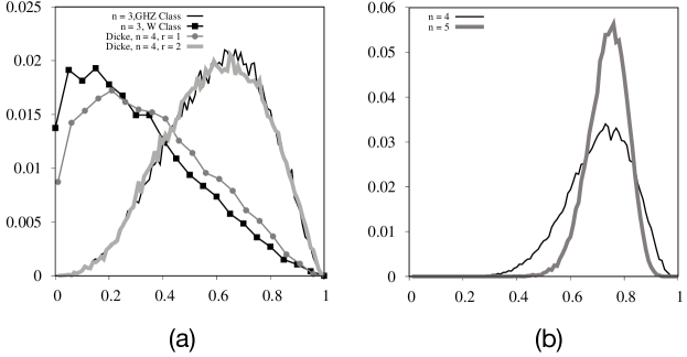
Figure 1: (Color online.) Absence of noise. Normalized frequency distribution, $f_{n}^{0}$ (vertical axis), against $E_{12}^{0}(n)$ (horizontal axis). We Haar uniformly generate random pure states with (a) $n=3$, (b) $n=4,5$ for studying $f_{n}^{0}$ . We also simulate three-qubit W class (a) and $4$-qubit generalized Dicke states with single and double excitations (a). The sample size is taken to be $5\times 10^{4}$ in each case. All quantities plotted are dimensionless.

III Distribution of localizable entanglement

As mentioned in Sec. I, random pure states with moderate values of $n$ are found to be highly entangled Hayden et al. (2006); Kendon et al. (2002) if one quantifies its entanglement via distance-based Horodecki et al. (2009); Shimony (1995); Wei and Goldbart (2003); Barnum and Linden (2001) or monogamy-based measures Rethinasamy et al. (2019). It is also noticed that von Neumann entropy of local density matrices of random multi-party pure states converges to unity for large number of parties Kendon et al. (2002). In this section, we address a similar question as to whether random pure states shared between moderate number of parties also possess high content of localizable entanglement. Such a question is non-trivial since LE is not straightforwardly a multi-party entanglement measure Gour and Spekkens (2006). Towards this aim, we first investigate the patterns of frequency distributions of LE for random multi-qubit pure states and its variation with the increase in number of qubits. We then study the effects of noise on the distributions after sending all the qubits through noisy channels.

III.1 Noiseless scenario

Our aim here is to examine LE over first two qubits of random pure multipartite states with a chosen seed measure, specifically EoF Wootters (1998); *wootters2001. A generic $n$-qubit pure state can be written as

$$\ket{\psi}=\sum_{j=0}^{2^{n}-1}a_{j}\ket{i_{1}}\ket{i_{2}}\cdots\ket{i_{n}}$$ (17)

with $\sum_{j=0}^{2^{n}-1}|a_{j}|^{2}=1$. Here, $\ket{i_{k}}\in\{\ket{0},\ket{1}\}$, $k=1,2,\cdots,n,$ form the computational basis of qubits $1$, $2$, $\cdots$, $n$. The state parameters $\{a_{j};j=0,1,\cdots,2^{n}-1\}$ are complex numbers having the form $a_{j}=\alpha_{j}+\text{i}\beta_{j}$, $j=0,1,\cdots,2^{n}-1$, where $\alpha_{j}$ and $\beta_{j}$ are real numbers. For Haar uniformly generated $n$-qubit pure states, values of $\alpha_{j}$ and $\beta_{j}$, $j=0,1,\cdots,2^{n}-1$, can be chosen from a Gaussian distribution of mean zero and standard deviation unity Bengtsson and Życzkowski (2006). In the case of three-qubit systems, random pure states generated in this fashion belong to the GHZ class of states Dür et al. (2000). We examine the normalized frequency distribution (NFD) of the values of localizable entanglement of formation, which we obtain by Haar uniformly generating random pure states of $n=3,4,$ and $5$ qubits, and computing $E_{12}^{0}(n)$ for each of these states for a fixed value of $n$. The normalized frequency is defined as Bulmer (1965)

$$f_{n}^{0}=\frac{N({E_{12}^{0}(n)})}{N_{S}},$$ (18)

where $N({E_{12}^{0}}(n))$ is the number of Haar uniformly generated random pure states of $n$ qubits having $E_{12}^{0}(n)$, and $N_{S}$ is the total number of the $n$-qubit states simulated, representing the sample size.

$n$	3 (W Class)	3 (GHZ Class)	4	5
$\left\langle E_{12}^{0}(n)\right\rangle$	0.31	$0.60$	$0.71$	$0.74$
$\sigma_{n}$	$0.22$	$0.18$	$0.12$	$0.07$
$\eta_{n}$	$0.61$	$-0.28$	$-0.46$	$-0.42$

Table 1: Noiseless scenario. Table for the mean, standard deviation, and skewness of the normalized frequency distributions in the case of random three- (the GHZ class), four-, and five-qubit states and the W class states. All quantities are dimensionless.

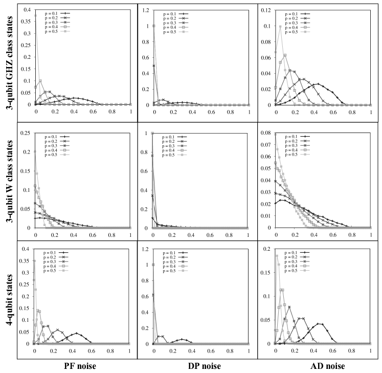
Figure 2: (Color online.) Normalized frequency distribution under local noise. Normalized frequency distribution, $f_{n}^{p}$ (vertical axes), vs. $E_{12}(n,p)$ (horizontal axes). Random pure states in the case of $n=3$ (GHZ and W class) and $4$ (from top to bottom horizontal panels) are subjected to phase-flip (left column), depolarizing (middle column), and amplitude-damping (right column) noise of strengths $p=0.1,0.2,0.3,0.4,$ and $0.5$. A sample of $N_{S}=5\times 10^{4}$ random pure initial ($p=0$) states are considered for each of the normalized frequency distributions. All quantities plotted are dimensionless.

The NFD of $E_{12}^{0}(n)$ in the case of three-, four-, and five-qubit systems are depicted in Fig. 1. As is evident from the shape of the distributions, the mean of the NFD, given by Bulmer (1965)

$$\left\langle E_{12}^{0}(n)\right\rangle=\sum_{E_{12}^{0}(n)}E_{12}^{0}(n)f_{n}^{0},$$ (19)

shifts towards $\left\langle E_{12}^{0}(n)\right\rangle=1$ as $n$ increases from $3$ to $5$, thereby satisfying

$$E_{12}^{0}(n_{1})>E_{12}^{0}(n_{2})$$ (20)

for $n_{1}>n_{2}$ with $n_{1},n_{2}\in\{3,4,5\}$. Note that the increment is considerably lower in the case of the change $n=4$ to $n=5$ as compared to the increment during the change $n=3$ to $n=4$. Interestingly however, the shapes of the distribution change drastically with the variation of $n$. To capture such feature of NFD, we compute the standard deviation (SD) Bulmer (1965),

$$\sigma_{n}=\left[\left\langle\left(E_{12}^{0}(n)\right)^{2}\right\rangle-\left(\left\langle E_{12}^{0}(n)\right\rangle\right)^{2}\right]^{\frac{1}{2}}.$$ (21)

Indeed, we find that the SD decreases remarkably as shown in Table 1, thereby showing more randomly generated states cluster around a large value of $\left\langle E_{12}^{0}\right\rangle$ with increasing $n$. We also notice that with increasing $n$, the distributions become more symmetric around the mean, which we confirm by studying skewness Bulmer (1965),

$$\eta_{n}=\sum_{E_{12}^{0}(n)}\left(\frac{E_{12}^{0}(n)-\left\langle E_{12}^{0}(n)\right\rangle}{\sigma}\right)^{3}f(E_{12}^{0}(n)),$$ (22)

of the NFD, tabulated in Table 1.

There exists another interesting class of three-qubit pure states, namely, the W class states Dür et al. (2000), a generic state of which has the form

$$\ket{\psi}=a_{0}\ket{001}+a_{1}\ket{010}+a_{2}\ket{100}+a_{3}\ket{000},$$ (23)

with $\sum_{l=0}^{3}|a_{l}|^{2}=1$. Similar to the case of the GHZ class states, the state parameters $\{a_{j};j=0,1,2,3\}$ here are also complex numbers $a_{j}=\alpha_{j}+\text{i}\beta_{j}$, $j=0,1,2,3$, with $\alpha_{j}$ and $\beta_{j}$ being real numbers. Other states in W class either belongs to the subspace represented by $\ket{\psi}$, or are local unitarily connected to a state in that subspace. From a three-qubit W class state having the form in Eq. (23), a GHZ class state can not be obtained via stochastic local operations and classical communication (SLOCC) in a single-copy level Dür et al. (2000). However, random W class states can be generated Haar uniformly by generating values of $\alpha_{j}$ and $\beta_{j}$, $j=0,1,2,3,$ from a Gaussian distribution of mean zero and standard deviation unity, which is a method similar to that for the GHZ class states.

Let us justify that the generation of W class states in the procedure described above is Haar uniform. The state parameters $\{a_{j};j=0,1,2,3\}$ are complex numbers $a_{j}=\alpha_{j}+\text{i}\beta_{j}$, $j=0,1,2,3$, where $\alpha_{j}$ and $\beta_{j}$ are real numbers. The parameters $\{\alpha_{j},\beta_{j}\}$ form an eight variable tuple, which we denote by $r=\{a_{j},b_{j}\}$, where $r\in\mathbb{R}^{8}$, the real space in eight dimension. The individual probability distributions corresponding to $a_{j}$ and $b_{j}$ can be written as $\phi(a_{j})=(2\pi)^{-1/2}\exp(-a^{2}_{j}/2)$ and $\phi(b_{j})=(2\pi)^{-1/2}\exp(-b^{2}_{j}/2)$, respectively, and the joint probability density function of $r$ reads as $f(r)=(2\pi)^{-4}\exp\left[-\sum_{i=1}^{4}(a^{2}_{j}+b^{2}_{j})/2\right]$, which equals to $(2\pi)^{-4}\exp\left[-\left\|r\right\|^{2}/2\right]$. Here, $f(r)$ is independent of the direction of $r$, but depends on the length of $\left\|r\right\|$, implying that $\hat{r}=\frac{r}{\left\|r\right\|}$ is uniformly distributed over $\mathbb{S}^{7}$, with $\mathbb{S}^{7}$ being seven-dimensional surface of unit sphere in $\mathbb{R}^{8}$, and we have considered normalization constraint in $\mathbb{R}^{8}$. It also implies that $\hat{r}$ follows the joint probability distribution $f(\hat{r})=\exp(-1/2)/\sqrt{(2\pi)^{8}}$, which remains constant over all directions, thereby suggesting that the generated states are Haar uniform in this subspace (see Ozols (2009)). In this paper, we consider localizable entanglement, which is invariant under local unitary transformation. Therefore, localizable entanglement of the Haar uniformly generated states of the form $\ket{\psi}$ in the generated subspace contains full information about the behaviour of LE for the complete state space of the entire W class. This also implies that the statistics corresponding to the localizable entanglement in the generated subspace faithfully represents the statistics of it in the entire state space of the W class.

The W class states with vanishing monogamy score for concurrence form a set of measure zero in the states space of three-qubits Dür et al. (2000), and hence they can not be found from the generation of three-qubit random states following the methodology descried in the discussion succeding Eq. (17). This can easily be seen from the fact that the generation of a generic state in the W class requires vanishing of a number of coefficients in the general form of a state in the GHZ class, which is not possible in the random Haar uniform generation Bengtsson and Życzkowski (2006) of GHZ class states having the form given in Eq. (17). However, states belonging to W class also possess certain features of entanglement, which make them useful for quantum information processing tasks Sen (De); *kaszlikowski2008; *barnea2015; *laskowski2015; *roy2018. We, therefore, separately generate the W class states by randomly choosing its parameters following the process described above, and determine the NFD of $E_{12}^{0}(n)$ (see Fig. 1) for comparison.

Depolarizing noise

$p=0.1$ $p=0.2$ $p=0.3$ $n$ $3$ $4$ $5$ $\left\langle E_{12}(n,p)\right\rangle$ $0.30$ $0.30$ $0.27$ $\sigma_{n}(p)$ $0.11$ $0.07$ $0.04$ $\eta_{n}(p)$ $-0.10$ $-0.28$ $-0.16$ $n$ $3$ $4$ $5$ $\left\langle E_{12}(n,p)\right\rangle$ $0.10$ $0.08$ $0.06$ $\sigma_{n}(p)$ $0.05$ $0.03$ $0.02$ $\eta_{n}(p)$ $0.29$ $0.30$ $0.36$ $n$ $3$ $4$ $5$ $\left\langle E_{12}(n,p)\right\rangle$ $0.01$ $0.01$ $0.00$ $\sigma_{n}(p)$ $0.01$ $0.01$ $0.00$ $\eta_{n}(p)$ $1.15$ $1.08$ $1.03$

Phase-flip noise

$p=0.1$ $p=0.2$ $p=0.3$ $n$ 3 4 5 $\left\langle E_{12}(n,p)\right\rangle$ $0.40$ $0.44$ $0.43$ $\sigma_{n}(p)$ $0.14$ $0.09$ $0.06$ $\eta_{n}(p)$ $-0.19$ $-0.28$ $-0.11$ $n$ 3 4 5 $\left\langle E_{12}(n,p)\right\rangle$ $0.24$ $0.25$ $0.25$ $\sigma_{n}(p)$ $0.10$ $0.06$ $0.05$ $\eta_{n}(p)$ $-0.04$ $-0.02$ $0.08$ $n$ 3 4 5 $\left\langle E_{12}(n,p)\right\rangle$ $0.13$ $0.13$ $0.13$ $\sigma_{n}(p)$ $0.06$ $0.04$ $0.03$ $\eta_{n}(p)$ $0.13$ $0.15$ $0.16$

Amplitude-damping noise

$p=0.1$ $p=0.2$ $p=0.3$ $n$ 3 4 5 $\left\langle E_{12}(n,p)\right\rangle$ $0.42$ $0.45$ $0.43$ $\sigma_{n}(p)$ $0.14$ $0.09$ $0.05$ $\eta_{n}(p)$ $-0.18$ $-0.34$ $-0.26$ $n$ 3 4 5 $\left\langle E_{12}(n,p)\right\rangle$ $0.28$ $0.27$ $0.24$ $\sigma_{n}(p)$ $0.11$ $0.07$ $0.04$ $\eta_{n}(p)$ $0.00$ $-0.10$ $-0.01$ $n$ 3 4 5 $\left\langle E_{12}(n,p)\right\rangle$ $0.18$ $0.15$ $0.12$ $\sigma_{n}(p)$ $0.08$ $0.05$ $0.03$ $\eta_{n}(p)$ $0.23$ $0.21$ $0.28$

White noise

$p=0.1$ $p=0.2$ $p=0.3$ $n$ 3 4 5 $\left\langle E_{12}(n,p)\right\rangle$ $0.46$ $0.55$ $0.57$ $\sigma_{n}(p)$ $0.15$ $0.10$ $0.06$ $\eta_{n}(p)$ $-0.26$ $-0.45$ $-0.41$ $n$ 3 4 5 $\left\langle E_{12}(n,p)\right\rangle$ $0.33$ $0.40$ $0.42$ $\sigma_{n}(p)$ $0.12$ $0.08$ $0.05$ $\eta_{n}(p)$ $-0.19$ $-0.42$ $-0.37$ $n$ 3 4 5 $\left\langle E_{12}(n,p)\right\rangle$ $0.23$ $0.28$ $0.30$ $\sigma_{n}(p)$ $0.09$ $0.06$ $0.04$ $\eta_{n}(p)$ $-0.07$ $-0.30$ $-0.27$

Table 2: Statistical quantities of the normalized frequency distributions under local and global noise. Tabulation of mean, standard deviation, and skewness of the normalized frequency distributions corresponding to the three-, four-, and five-qubit random pure states subjected to the depolarizing, phase-flip, amplitude-damping, and white noise for noise strengths given by $p=0.1,0.2,0.3$. The sample size considered for the determination of the metrics is $N_{S}=5\times 10^{4}$ for each of the cases. All quantities are dimensionless.

We find that the NFD of $E_{12}^{0}(n)$ in the case of states belonging to three-qubit $W$ class is qualitatively different from the GHZ class, as is evident from Fig. 1. In contrast to the high value $(>0.5)$ of the mean of the NFD in the case of the GHZ class, $\langle E_{12}^{0}(n)\rangle$ has a comparatively lower value for the states from the W class. It is also clear from Fig. 1 that the shapes of the distributions obtained from these two classes are strikingly different which can be confirmed from the values of the SD and the skewness of the respective NFDs (see Table 1). It also indicates that the distributions derived from the states belonging to the set of measure zero can show certain trait that cannot be seen for random pure states. This result is similar to the difference between the GHZ and the W class states in terms of the monogamy scores Giorgi (2011); *prabhu2012; *dhar2017 of quantum correlation measures, which are also considered to be multiparty in nature. This also strengthens the potential of the LE computed over a pair of qubits to be considered as a multiparty measure of entanglement.

The above discussion indicates that it can also be interesting to investigate the distribution of LE for a certain family of states with higher number of qubits. For high value of $n$, several such family of states exists. For our investigation, we randomly generate four-qubit genneralized Dicke states Dicke (1954); *kumar2017; *bergmann2013; *lucke2014; *chiuri2012 with a single and double excitations, given by

$$\ket{\psi_{n}^{r}}=\sum_{i}a_{i}\mathcal{P}_{i}\left[\ket{0}^{\otimes n-r}\ket{1}^{\otimes r}\right],$$ (24)

with $a_{i}=\alpha_{i}+\text{i}\beta_{i}$ being complex numbers ($\alpha_{i},\beta_{i}$ are real numbers chosen from normal distributions of vanishing mean and unit SD – a procedure similar to the case of the random $n$-qubit pure states and the three-qubit W class states) such that $\sum_{i}|a_{i}|^{2}=1$, and the summation in Eq. (24) being over all possible permutations, $\{\mathcal{P}_{i}\}$, of the product state $\ket{0}^{\otimes n-r}\ket{1}^{\otimes r}$ having $r$ qubits in the excited state, $\ket{1}$, and the rest of the qubits in the ground state, $\ket{0}$. Like the W class states, these Dicke states also form a set of measure zero in the state-space of four-qubit systems for a reason similar to that in the case of the three-qubit W class states. Moreover, the Haar uniformity of these randomly generated Dicke states can also be proven via a procedure similar to that in the case of W states. We observe that the NFD of $E_{12}^{0}(n)$ corresponding to random pure states of the form (24) with $n=4$, $r=1$ is similar to that of the W class states, as in Fig. 1, while the same corresponding to $n=4$, $r=2$ has a different shape which is almost identical to the NFD corresponding to the three-qubit GHZ class states. With respect to the above observation, we also notice that in the case of the three-qubit GHZ class states and the four-qubit Dicke states with two excitations, post-measurement states of the two qubits on which entanglement is localized, correspondoing to the optimal measurement set-up, in both the cases have comparable non-zero values of entanglement. On the other hand, in the case of the three-qubit W class states, only one of the two-qubit post-measurement states corresponding to the optimal measurement has non-zero entanglement value, while the other post-measurement state has almost vanishing entanglement. This is similar to the case of the four-qubit Dicke states with one excitation, where corresponding to the optimal measurement setting, only one of the post-measurement states have non-zero entanglement while the entanglement values fo the other post-measurement two-qubit states vanish.

III.2 Effects of noise

Upto now, distribution of LE has been considered for Haar uniformly chosen multi-qubit quantum states in a noiseless scenario. However, in a realistic situation, a multi-party state, shared between several parties at different locations, can almost always be affected by noise. It is, therefore, of practical interest to check how the above results are modified in presence of different types of noise. In order to observe the consequence of noise on the distribution of LE, we first generate random pure states $\rho_{0}=\ket{\psi}\bra{\psi}$ of three-, four- and five-qubits. Then, all the qubits are affected by a specific noisy channel, as described in Sec. II.2. Specifically, for a fixed value of the noise parameter $p$, we determine the NFD of $E_{12}(n,p)$ given by

$$f_{n}^{p}=\frac{N({E_{12}(n,p)})}{N_{S}},$$ (25)

where we compute $E_{12}(n,p)$ as mentioned earlier (see discussion succeeding Eq. (18)). Similar to the noiseless scenario, in the case of three-qubit systems, we separately generate the pure states belonging to the W class, and investigate the effect of noise on LE in these states, as presented in the subsequent discussion.

Depolarizing noise NFD Metric $p=0.1$ $p=0.2$ $p=0.3$ $p=0.4$ $p=0.5$ $\left\langle E_{12}(n,p)\right\rangle$ $0.15$ $0.05$ $0.01$ $0.00$ $0.00$ $\sigma_{n}(p)$ $0.13$ $0.06$ $0.01$ $0.00$ $0.00$ $\eta_{n}(p)$ $0.82$ $1.27$ $2.44$ $15.45$ $0.00$	Phase-flip noise NFD Metric $p=0.1$ $p=0.2$ $p=0.3$ $p=0.4$ $p=0.5$ $\left\langle E_{12}(n,p)\right\rangle$ $0.23$ $0.16$ $0.10$ $0.06$ $0.03$ $\sigma_{n}(p)$ $0.16$ $0.11$ $0.07$ $0.04$ $0.02$ $\eta_{n}(p)$ $0.62$ $0.64$ $0.67$ $0.68$ $0.72$
Amplitude-damping noise NFD Metric $p=0.1$ $p=0.2$ $p=0.3$ $p=0.4$ $p=0.5$ $\left\langle E_{12}(n,p)\right\rangle$ $0.26$ $0.21$ $0.17$ $0.13$ $0.10$ $\sigma_{n}(p)$ $0.18$ $0.15$ $0.13$ $0.10$ $0.07$ $\eta_{n}(p)$ $0.63$ $0.67$ $0.72$ $0.74$ $0.79$	White Noise NFD Metric $p=0.1$ $p=0.2$ $p=0.3$ $p=0.4$ $p=0.5$ $\left\langle E_{12}(n,p)\right\rangle$ $0.25$ $0.18$ $0.13$ $0.08$ $0.04$ $\sigma_{n}(p)$ $0.18$ $0.15$ $0.12$ $0.08$ $0.05$ $\eta_{n}(p)$ $0.66$ $0.76$ $0.91$ $1.10$ $1.45$

Table 3: Metrics of the normalized frequency distributions for states from three-qubit W class under noise. Tabulation of the mean, standard deviation, and skewness of the normalized frequency distributions corresponding to the three-qubit random pure states belonging to the W class, subjected to the depolarizing, phase-flip, amplitude-damping, and white noise for five specific noise strengths given by $p=0.0,0.2,0.3,0.4,$ and $0.5$. The sample size is same as Table 2. All quantities are dimensionless.

We first concentrate on the three-qubit GHZ class along with the Haar uniformly generated random pure states of four- and five-qubits, subjected to local noise. For $p>0$, we evaluate $f_{n}^{p}$ for fixed values of $p$, with $n=3,4,5$. The profiles of $f_{n}^{p}$ corresponding to $n=3,4$, for five different noise strengths $p=0.1,0.2,0.3,0.4,0.5$, and for the different types of noise (see Sec. II.2) are depicted in Fig. 2, while the metrics of the NFDs are tabulated in Table 2. The profile of $f_{n}^{p}$ corresponding to $n=5$ are similar to that of $n=4$, and the GHZ class states for $n=3$. Since the local noise considered in this paper are Markovian, one expects $E_{12}(n,p_{2})\leq E_{12}(n,p_{1})\leq E_{12}^{0}(n)$, where $1\geq p_{2}\geq p_{1}\geq 0$, for a fixed value of $n$. In agreement with this, for a fixed $n$, the mean, $\left\langle E_{12}(n,p)\right\rangle$, of the NFDs satisfy

$$\left\langle E_{12}(n,p_{2})\right\rangle\leq\left\langle E_{12}(n,p_{1})\right\rangle\leq\left\langle E_{12}^{0}(n)\right\rangle$$ (26)

for $1\geq p_{2}\geq p_{1}\geq 0$, and the peak of the distribution shifts towards lower values of $E_{12}(n,p)$ with increasing $p$, as is evident from Fig. 2. On the other hand, for a fixed $p$, we interestingly find

$$\left\langle E_{12}(n_{1},p)\right\rangle\approx\left\langle E_{12}(n_{2},p)\right\rangle$$ (27)

for $n_{1}>n_{2}$, $n_{1},n_{2}\in\{3,4,5\}$, for a specific type of noise, where the difference between $\left\langle E_{12}(n_{1},p)\right\rangle$ and $\left\langle E_{12}(n_{2},p)\right\rangle$ occurring only in the second decimal place. This is in sharp contrast to the finding for the noiseless scenario, as summarized in Eq. (20). The values of the SD, $\sigma_{n}^{p}$ (with a definition similar to that in Eq. (21) with a non-zero $p$), of the NFDs are found to satisfy

$$\sigma_{n}(p_{1}) \geq \sigma_{n}(p_{2})\;\text{for}\;1\geq p_{2}>p_{1}\geq 0,$$

$$\sigma_{n_{1}}(p) \geq \sigma_{n_{2}}(p)\;\text{for}\;n_{2}>n_{1};\;n_{1},n_{2}\in\{3,4,5\},$$ (28)

for a fixed type of noise.

We now move on to the comparison of LE between different noise models. While DP noise turns out to be the most stringent in pushing the average value of LE towards zero, interestingly, considerably high values of localizable entanglement sustain for the AD noise when the same noise strength $p$ as in the case of the DP and the PF noise is applied. This is clearly visible from the plots in Fig. 2 and Table 2. Also, the values of the metrics as well as the profiles of the NFDs suggest that the effect of noise on the distribution of LE is qualitatively similar for the PF and the AD channels, while being considerably different from the same corresponding to the DP channel. In order to obtain a full picture about the complete state-space of the three-qubit system, we separately generate three-qubit states belonging to the W class, and perform the same analysis as in the case of states belonging to the three-qubit GHZ class (see Fig. 2 and Table 2). The profiles of the NFDs clearly indicate a higher robustness of the multi-qubit quantum states of three- (including the GHZ and the W class states), four-, and five-qubits towards AD noise as far as the value of LE is concerned, in comparison to the PF and the DP noise. We will present a more quantitative analysis on this topic in Sec. IV. In order to check how the NFDs corresponding to the zero-measure states for $n>3$ response against local noise, we apply PF, DP, and AD noise on the qubits of four-qubit generalized Dicke states with single and double excitations (Eq. (24)), and determine the NFDs of $E_{12}(n,p)$ for different values of $p>0$ for each of the noise-types. We find that our observation regarding the difference between the shapes of the NFDs corresponding to the Dicke states with single and double excitations in noiseless case holds in the noisy scenario also.

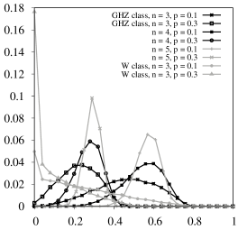
Figure 3: (Color online.) Normalized frequency distribution under white noise. $f_{n}^{p}$ (vertical axes) with respect to $E_{12}(n,p)$ (horizontal axes). Random pure states in the case of $n=3,4,5$, and the three-qubit W class states are affected by white noise of strengths $p=0.1,0.3$. The sample size is the same as in Fig. 2. All quantities plotted are dimensionless.

To see the effect of global noise, we investigate the profiles of NFDs for a specific noise strengths as depicted in Fig. 3). Comparing Tables 2 and 3, the states in the GHZ class are more robust to the white noise than that from the W class. Similar to the local noise, here also we observe that for fixed noise strength, mean and SD of NFDs do not change with the increase of $n$ (see Table 2).

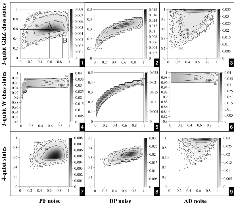
Figure 4: (Color online.) Contour map of $E_{L}^{0}$ and $p_{c}$ under local noise. The rows and columns of the figure and the sample size used to generate the data are the same as in Fig. 2. The values of $f\left(E_{12}^{0}(n),p_{c}\right)$ corresponding to the different contour lines are as follows. [1],[7]: $10^{-3}$ (i), $10^{-4}$ (ii), $10^{-5}$ (iii), from inside to outside, [2-6,8,9]: $10^{-2}$ (i), $10^{-3}$ (ii), $10^{-4}$ (iii), $10^{-5}$ (iv), from inside to outside. All quantities plotted are dimensionless.

IV Robustness against noise

We have pointed out that the effect of noise on the distribution of localizable entanglement is qualitatively similar for the PF and the AD channels, although LE seems to survive against more noise in the case of the AD channel. In this section, we aim for an unambiguous conclusion on the robustness of a multi-qubit quantum state, in terms of its LE, against different types of noise. In order to formulate a figure of merit for this purpose, we look at two specific quantities – (1) the initial value of localizable entanglement, $E_{12}^{0}(n)$, of the $n$-qubit state, and (2) the value of noise strength, $p_{c}$, which we refer to as the critical strength of noise, such that

$$E_{12}(n,p) > 0,\text{for }p<p_{c},$$

$$E_{12}(n,p) = 0,\text{for }p\geq p_{c},$$ (29)

provided $E_{12}^{0}(n)>0$. Whether a high (low) value of $E_{12}^{0}(n)$ implies a high (low) value of $p_{c}$, or whether $p_{c}$ has any other functional dependence on the value of $E_{12}^{0}(n)$, are non-trivial questions, and need careful consideration for a quantitative analysis of the robustness of localizable entanglement against noise.

Towards this goal, we Haar uniformly simulate a sample of random pure states of size $N_{S}$ for each of the three-, four-, five-qubit systems, and apply different types of local as well as global noise on the qubits. We define the normalized frequency

$$f\left(E_{12}^{0}(n),p_{c}\right)=\frac{N(E_{12}^{0}(n),p_{c})}{N_{S}},$$ (30)

where $N(E_{12}^{0}(n),p_{c})$ is the number of Haar uniformly generated random pure states with $E_{L}^{0}(n)$ satisfying Eq. (29) for a system of $n$ qubits. For $N_{S}=5\times 10^{4}$, we plot $f\left(E_{12}^{0}(n),p_{c}\right)$ as functions of $E_{12}^{0}(n)$ and $p_{c}$ in Fig. 4 for Haar uniformly generated three- and four-qubit random pure states subjected to local noise, where the bin size for determining $f\left(E_{12}^{0}(n),p_{c}\right)$ is taken to be $10^{-1}\times 10^{-1}$. The observations emerging from Fig. 4 are as follows.

(1) In the case of random pure multi-qubit $(n=3,4,5)$ states with a fixed initial value of $E_{12}^{0}(n)$, there can be a number of values of $p_{c}$, as indicated from the vertical spreads of the $f\left(E_{12}^{0}(n),p_{c}\right)$ in Fig. 4. It clearly indicates that the critical value of noise-strength is independent of the content of the LE of the initial state. Also, a relatively low value of $E_{12}^{0}(n)$ may correspond to a higher value of $p_{c}$ compared to the same for a high value of $E_{12}^{0}(n)$ – see, for example, the points A and B in the case of three-qubit GHZ class states under PF noise.

(2) There is a qualitative difference between the landscape of $f\left(E_{12}^{0}(n),p_{c}\right)$ in the case of three-qubit GHZ and W class states under PF noise. While the former indicates existence of the values of $E_{12}^{0}(n)$ and $p_{c}$ over a broad range in the region $0\leq E_{12}^{0}(n)\leq 1$, $0\leq p_{c}\leq 1$, in the latter, most of the values of $p_{c}$ are confined in the range $0.9\leq p_{c}\leq 1$, while the values of $E_{12}^{0}(n)$ is consistent with the profiles of the NFD corresponding to the three-qubit W class states in the noiseless situation (see Fig. 1).

(3) The NFDs, $f\left(E_{12}^{0}(n),p_{c}\right)$, corresponding to the three- (GHZ class), four-, and five-qubit random pure states under local noise exhibit qualitatively similar trend. The concentration of the randomly chosen states shifts towards higher values of $E_{12}^{0}(n)$ when $n$ increases, which is consistent with the findings in Sec. III.1 (see Eq. (20) and Fig. 1).

(4) As predicted in Sec. III.2, the DP noise turns out to be the most destructive one, which is evident from the considerably low values of $p_{c}$ irrespective of the values of $E_{12}^{0}(n)$, among all types of local noise as well as white noise and random initial states.

(5) In the case of the AD noise, irrespective of the values of $E_{12}^{0}(n)$, the values of $p_{c}$ for majority of the three-qubit W class random pure states are found to be in the range $0.9\leq p_{c}\leq 1$ – a feature similar to the W class states under PF noise. On the other hand, for the three-qubit GHZ class states, the four- and the five-qubit random pure states under AD noise, there is a large fraction of states for which $p_{c}\in[0.9,1]$, although there are fraction of states scattered over $0\leq p_{c}<0.9$. This indicates (1) a higher robustness of LE of multi-qubit random three-qubit pure states belonging to the W class under the influence of AD and PF noise, and (2) a higher robustness of LE of a large fraction of three-qubit GHZ class states as well as four- and five-qubit random pure states under AD noise. These findings are in a good agreement with the inference in Sec. III.2.

The trends of the NFD, $f\left(E_{12}^{0}(n),p_{c}\right)$, corresponding to the three-, four-, and five-qubit random pure states under white noise is similar to the DP noise, which is shown in Fig. 4. In all other cases, the change in the landscape is as per the change in the distribution of $E_{12}^{0}(n)$ when $n$ increases from $3$ to $5$ (see Fig. 3).

Let us now check the status of $p_{c}$ of two important families of three-qubit states, namely, the generalized GHZ Greenberger et al. (1989) and generalized W Zeilinger et al. (1992); Dür et al. (2000) states. The former is defined as

$$\ket{\psi}=a_{0}\ket{000}+a_{1}\ket{111},$$ (31)

with $|a_{0}|^{2}+|a_{1}|^{2}=1$, $a_{0}$ and $a_{1}$ being complex numbers having the form $a_{j}=\alpha_{j}+\text{i}\beta_{j}$, $j=0,1$, where $\alpha_{j}$ and $\beta_{j}$ are real numbers. On the other hand, a three-qubit generalized W state $\ket{\psi}$ has the form

$$\ket{\psi}=a_{0}\ket{001}+a_{1}\ket{010}+a_{2}\ket{100},$$ (32)

with $\sum_{j=0}^{2}|a_{j}|^{2}=1$. The state parameters $a_{j}$, $i=0,1,2$, are complex numbers having the form $a_{j}=\alpha_{j}+\text{i}\beta_{j}$, $j=0,1,2$, where $\alpha_{j}$ and $\beta_{j}$ are real numbers. Specifically, here we see whether the generalized GHZ and W states exhibit behaviours different than those shown by the GHZ class and the W class states respectively, under the application of noise. Towards this aim, we investigate the variation of the values of $p_{c}$ against that of $E_{12}^{0}(n)$ for the generalized GHZ and the W states subjected to local noise channels. We find that the trends of $p_{c}$ as a function of $E_{12}^{0}(n)$ are similar, qualitatively as well as quantitatively, for the generalized W states and the states belonging to the W class for all the three types of noise. However, such similarities are not always present between the generalized GHZ states and the states from the GHZ class. Let us denote the critical noise strength $p_{c}$ corresponding to a generalized GHZ state having initial LE $E_{12}^{0}(n)$ by $p_{c}^{(1)}$, and the same corresponding to a GHZ class state having the same initial LE $E_{12}^{0}(n)$ by $p_{c}^{(2)}$. In the case of the PF channel and for all values of $E_{12}^{0}(n)$, for majority of the GHZ class states, $p_{c}^{(2)}\leq p_{c}^{(1)}$, while in the case of the DP noise, there exists considerable number of states in GHZ class for which $p_{c}^{(2)}\geq p_{c}^{(1)}$ for all $E_{12}^{0}(n)$. For DP noise, the fraction of states in GHZ class for which $p_{c}^{(2)}\geq p_{c}^{(1)}$ increases with increasing $E_{12}^{0}(n)$. The results again confirms that the properties of random pure states cannot be mimicked by a family or subset of states.

V Conclusion

To summarize, we investigated whether multi-qubit random pure states can exhibit high values of localizable entanglement (LE) concentrated over a chosen pair of qubits. Due to the computational limitation imposed by the difficulty in achieving the maximization involved in the definition of localizable entanglement, we have restricted our study in systems composed of three-, four-, and five-qubits. By determining the normalized frequency distributions, we showed that for Haar uniformly generated random pure states, the average value of localizable entanglement increases with increasing the number of qubits in the system. Also, high clustering of the randomly generated multi-qubit quantum states around higher values of localizable entanglement is signalled by other metrics of the normalized frequency distribution, such as the standard deviation and the skewness. This feature bears similarity with the characteristics of genuine multi-party entanglement as shown in previous works. It also indicates that LE can mimic properties similar to a valid multi-party entanglement measure.

In order to check how this characteristic changes in a realistic scenario when noise is introduced in the system, we apply phase-flip, depolarizing, amplitude damping, and white noises on the Haar uniformly simulated random pure states of three-, four-, and five-qubit systems, and study the variation of the metrics of the normalized frequency distribution with varying noise strength. We found that the mean of LE does not increase with the increase of the number of parties for a fixed noise strength. Instead, it remains almost constant for a fixed value of noise which is in contrast with the noiseless situation. Such a feature is independent of the choices of noise models considered in this paper. Investigation also reveals that amplitude damping channel destroys less LE compared to any other channels. Moreover, we find that the critical noise strength above which LE vanishes does not depend on the initial LE of a given state. For the amplitude and phase damping noise, the analysis of LE shows that the states from the W class is more robust than that from the GHZ class.

Our analysis also reveals that under decoherence, nature of entanglement content of most of the multi-qubit states are similar and not maximal unlike the noiseless scenario. If such patterns in presence of noise persists for other multi-party entanglement measures, they may be useful for quantum computational speed-up, especially in a realistic scenario. Our study also highlights the potential of localizable entanglement to be considered as an appropriate candidate in revealing the multi-party nature of quantum correlation present in a composite quantum system, and motivates extensive research in this direction from the perspective of quantum information processing tasks.