On Calibration of a Nominal Structure–Property Relationship Model for
Chiral Sculptured Thin Films by Axial Transmittance Measurements

J. A. Sherwin¹, A. Lakhtakia¹ and I. J. Hodgkinson²

¹CATMAS — Computational and Theoretical Materials Science Group
Department of Engineering Science and Mechanics
Pennsylvania State University, University Park, PA 16802–6812

²University of Otago, Department of Physics
PO Box 56, Dunedin, New Zealand

ABSTRACT–A chiral sculptured thin film is fabricated from patinal titanium oxide using the serial bideposition technique. Axial transmittance spectrums are measured over a spectral region encompassing the Bragg regime for axial excitation. The same spectrums are calculated using a nominal structure–property relationship model and the parameter space of the model is explored for best fits of the calculated and measured transmittances. Ambiguity arising on calibrating the model against axial transmittance measurements is shown to be resolvable using non–axial transmittance measurements.

Key words: Bruggeman formalism, chiral sculptured thin film, circular Bragg phenomenon, model calibration, structure–properties relationship model, transmittance measurements

1 INTRODUCTION

Among the nano–engineered materials recently identified by the US National Research Council in a 1999 survey entitled Condensed–Matter and Materials Physics, Basic Research for Tomorrow’s Technology as significant for scientific and technological progress in the following two decades are sculptured thin films (STFs) [1, 2]. These nanostructured inorganic materials with unidirectionally varying properties can be designed and realized in a controllable manner using physical vapor deposition [3]–[8]. The ability to virtually instantaneously change the growth direction of their columnar morphology, through simple variations in the direction of the incident vapor flux, leads to a wide variety of microscopic columns with two–or three–dimensional shapes.

At visible and infrared wavelengths, a single–section STF is a unidirectionally nonhomogeneous continuum with direction–dependent properties [9]. Several sections can be grown consecutively into a multisection STF [1, 8]. Chiral STFs display the circular Bragg phenomenon in accordance with their periodic nonhomogeneity along the thickness direction. This phenomenon has been exploited to design, fabricate and test: circular polarization filters and laser mirrors, polarization–discriminatory handedness–inverters, and spectral hole filters [2, 4]. Furthermore, the porosity of STFs makes them attractive for fluid concentration sensing applications, as their optical response properties change in accordance with the number density of infiltrant molecules, which has been demonstrated theoretically as well as experimentally with chiral STFs [10]. Other optical, electronic, thermal, and biophysical applications are also under investigation by many researchers [2, 4], and the future of STFs continues to appear bright.

As STF technology matures from the proof–of–concept stage towards the marketable–devices stage, experimentalists as well as theorists are increasingly challenged to control and optimize the morphological and other characteristics of chiral STFs for economically attractive applications. On the one hand, the recently developed serial bideposition (SBD) technique [11] is ideally suited for this purpose. It yields chiral STFs with controlled morphology to enhance the so–called local linear birefringence and optical activity. On the other hand, a nominal model for structure–property relationships of chiral STFs has been devised [12, 13] and qualitatively tested [10].

In this communication, we report our first attempt at the calibration of the nominal microscopic–to–macroscopic model against transmittance spectrums measured when a chiral STF is excited by a plane wave along its direction of nonhomogeneity. The plan of this paper is as follows: The nominal model of a chiral STF as an ensemble of ellipsoids is briefly outlined in section 2. Model calibration involving the theoretical calculation of axial transmittances and the experimental setup for their measurement are outlined in section 3. Section 4 comprises the determination of model parameters, a discussion of the ambiguity when calibrating against axial transmittance measurements, and the potential resolution of the ambiguity by non–axial transmittance measurements. An $\exp(-i\omega t)$ time–dependence is assumed henceforth. All vectors are underlined once and all dyadics are underlined twice.

2 NOMINAL MODEL

As any STF comprises clusters that are electrically small at optical and lower frequencies, it can be considered as a material continuum at those frequencies [1, 9]. Furthermore, STFs have a locally columnar morphology with many void regions [3]–[8] — which leads naturally to the concept of local homogenization in order to construct continuum models. In our model, the deposited material as well as the void regions are nominally conceived as confocal parallel ellipsoids in any plane parallel to the substrate. The Bruggeman formalism is then used to estimate a reference permittivity dyadic in terms of two shape factors of the ellipsoids, the bulk constitutive properties of the deposited material, and the porosity. Infiltration of the void regions by some material can be handled by this model as also the frequency–dependence of the constitutive properties of the deposited materials. Calibration against experimental data is an essential feature of this model. As it has been discussed in detail elsewhere [13], we give only a brief outline here.

2.1 Constitutive Relations

The frequency–domain constitutive relations of a chiral STF (after homogenization) are given by

$$\underline{D}\left(\underline{r}\right) =\varepsilon_{0}\,\underline{\underline{\varepsilon}}\left(z\right)\mbox{ \tiny{${}^{\bullet}$} }\underline{E}\left(\underline{r}\right),$$ (1)

$$\underline{B}\left(\underline{r}\right) =\mu_{0}\,\underline{H}\left(\underline{r}\right),$$ (2)

where $\varepsilon_{0}$ and $\mu_{0}$ are the permittivity and permeability of free space (i.e., vacuum). The nonhomogeneous relative permittivity dyadic $\underline{\underline{\varepsilon}}$ is written in terms of a homogeneous permittivity dyadic $\underline{\underline{\varepsilon}}_{ref}^{o}$ and two rotation dyadics as

$$\underline{\underline{\varepsilon}}\left(z\right)=\underline{\underline{S}}_{z}\left(z\right)\mbox{ \tiny{${}^{\bullet}$} }\underline{\underline{S}}_{y}\left(\chi\right)\mbox{ \tiny{${}^{\bullet}$} }\underline{\underline{\varepsilon}}_{ref}^{o}\mbox{ \tiny{${}^{\bullet}$} }\underline{\underline{S}}_{y}^{-1}\left(\chi\right)\mbox{ \tiny{${}^{\bullet}$} }\underline{\underline{S}}_{z}^{-1}\left(z\right).$$ (3)

Here,

$$\underline{\underline{\varepsilon}}_{ref}^{o} = \varepsilon_{a}\underline{u}_{z}\underline{u}_{z}+\varepsilon_{b}\underline{u}_{x}\underline{u}_{x}+\varepsilon_{c}\underline{u}_{y}\underline{u}_{y},$$

$$= n_{1}^{2}\underline{u}_{x}\underline{u}_{x}+n_{2}^{2}\underline{u}_{z}\underline{u}_{z}+n_{3}^{2}\underline{u}_{y}\underline{u}_{y},$$

$$\underline{\underline{S}}_{y}\left(\chi\right) = \underline{u}_{y}\underline{u}_{y}+\left(\underline{u}_{x}\underline{u}_{x}+\underline{u}_{z}\underline{u}_{z}\right)\cos\chi+\left(\underline{u}_{z}\underline{u}_{x}-\underline{u}_{x}\underline{u}_{z}\right)\sin\chi,$$ (5)

$$\underline{\underline{S}}_{z}\left(z\right) = \underline{u}_{z}\underline{u}_{z}+\left(\underline{u}_{x}\underline{u}_{x}+\underline{u}_{y}\underline{u}_{y}\right)\cos\left(\pi z/\Omega\right)+h\left(\underline{u}_{y}\underline{u}_{x}-\underline{u}_{x}\underline{u}_{y}\right)\sin\left(\pi z/\Omega\right),$$ (6)

$2\Omega$ is the structural period, the angle of rise $\chi$ describes the elevation of the helicoidal columns above the $xy$ plane, whilst $n_{1,2,3}$ are the principal indexes of refraction [14]. The structural handedness parameter $h=1$ for right– and $h=-1$ for left–handed STFs. As the period is fixed a priori by the deposition conditions, $\underline{\underline{\varepsilon}}(z)$ can be completely delineated, provided that the reference permittivity dyadic

$$\underline{\underline{\varepsilon}}_{ref}=\underline{\underline{S}}_{y}\left(\chi\right)\mbox{ \tiny{${}^{\bullet}$} }\underline{\underline{\varepsilon}}_{ref}^{o}\mbox{ \tiny{${}^{\bullet}$} }\underline{\underline{S}}_{y}^{-1}\left(\chi\right)$$ (7)

is known.

2.2 Local Homogenization

Consider a homogenized composite medium (HCM) whose relative permittivity dyadic $\underline{\underline{\varepsilon}}_{HCM}$ is identical to that of the chosen chiral STF in the limit $\Omega\to\infty$, i.e., $\underline{\underline{\varepsilon}}_{HCM}=\underline{\underline{\varepsilon}}_{ref}$. The longest principal axes of all ellipsoids in this HCM are aligned parallel to the unit vector $\underline{u}^{\prime}_{x}=\underline{\underline{S}}_{y}\left(\chi\right)\mbox{ \tiny{${}^{\bullet}$} }\underline{u}_{x}$, while the smaller of the two remaining principal axes is aligned parallel to the unit vector $\underline{u}^{\prime}_{z}=\underline{\underline{S}}_{y}\left(\chi\right)\mbox{ \tiny{${}^{\bullet}$} }\underline{u}_{z}$. The deposited material is isotropic in bulk with relative permittivity scalar $\varepsilon_{s}$ — which can be considered in our model as frequency–dependent — while the relative permittivity of the void regions $\varepsilon_{v}$ equals unity, of course. With respect to its centroid, the surface of an ellipsoid may be described in cartesian coordinates by the relation

$${z^{\prime}}^{2}+\left(\frac{y^{\prime}}{\gamma_{2}}\right)^{2}+\left(\frac{x^{\prime}}{\gamma_{3}}\right)^{2}=\delta^{2},$$ (8)

where $\delta$ is a linear measure of the absolute size, while the transverse aspect ratio $\gamma_{2}>1$ and the slenderness ratio $\gamma_{3}>>1$ relate the three principal axes.

The Bruggeman formalism involves the solution of the dyadic equation [15]

$$f\,\underline{\underline{a}}_{s}+(1-f)\,\,\underline{\underline{a}}_{v}=\underline{\underline{0}}\,,$$ (9)

where $f$, ($0\leq f\leq 1$), is the volume fraction of the film occupied by the deposited material and $\underline{\underline{0}}$ is the null dyadic. The polarizability dyadics $\underline{\underline{a}}_{s,v}$ are explicit functions of $\varepsilon_{s,v}$, $\chi$, and $\gamma_{2,3}$, and implicitly depend on $\underline{\underline{\varepsilon}}_{ref}$ as well. Standard iterative methods detailed elsewhere [13] are used to compute $\underline{\underline{\varepsilon}}_{ref}$.

3 CALIBRATION OF THE NOMINAL MODEL

Our first attempt to calibrate the described model involves the excitation of a chiral STF by a normally incident plane wave, and the measurement of the consequent transmittances.

3.1 Axial Excitation

Let the region $0\leq z\leq L$ be occupied by a chiral STF while the regions $z\geq L$ and $z\leq 0$ are vacuous. An arbitrarily polarized plane wave, with wavenumber $k_{0}=\omega\sqrt{\varepsilon_{0}\mu_{0}}$ and wavelength $\lambda_{0}=2\pi/k_{0}$, is normally incident on the chiral STF from the lower half–space $z\leq 0$. This results in a plane wave reflected back into the lower half–space, and a plane wave transmitted into the upper half–space. The electric field phasor in the lower half–space is given by

$$\underline{E}\left(\underline{r}\right) =\left(a_{L}\,\underline{u}_{+}+a_{R}\,\underline{u}_{-}\right)e^{ik_{0}z}+\left(r_{L}\,\underline{u}_{-}+r_{R}\,\underline{u}_{+}\right)e^{-ik_{0}z};\quad z\leq 0\,,$$ (10)

where $\underline{u}_{\pm}=\left(\underline{u}_{x}\pm i\underline{u}_{y}\right)/\sqrt{2}$. The transmitted electric field has the phasor representation

$$\underline{E}_{tr}\left(\underline{r}\right) =\left(t_{L}\,\underline{u}_{+}+t_{R}\,\underline{u}_{-}\right)e^{ik_{0}\left(z-L\right)};\quad z\geq L\,.$$ (11)

The quantities $a_{L}$ and $a_{R}$ are the amplitudes of the left and right circularly polarized (LCP and RCP) components of the incident plane wave, while $r_{L,R}$ and $t_{L,R}$ are the analogous amplitudes of the reflected and transmitted planewave components.

A boundary value problem can be solved for the reflection and transmission amplitudes in terms of the incidence wave amplitudes, as discussed elsewhere in detail [9]. For our present purposes, the results are compactly written in matrix form as

$$\left[\begin{matrix}t_{L}\\ t_{R}\end{matrix}\right]=\left[\begin{matrix}t_{LL}&t_{LR}\\ t_{RL}&t_{RR}\end{matrix}\right]\left[\begin{matrix}a_{L}\\ a_{R}\end{matrix}\right].$$ (12)

Of the 4 coefficients appearing in the foregoing $2\times 2$ matrix, those with both subscripts identical refer to co-polarized, while those with two different subscripts refer to cross-polarized, transmission.

3.2 Experimental setup

Chiral STFs were grown by SBD using Patinal titanium oxide S granules. The details of SBD are discussed elsewhere [4, 16]. It suffices to note here that vapor is incident from a single source under free streaming conditions at the deposition angle $\chi_{v}$ (with respect to the substrate). The deposition angle can assume any value in the range $0^{\circ}<\chi_{v}\leq 90^{\circ}$, but is typically set between $20^{\circ}$ and $30^{\circ}$. The resultant morphology of the chiral STFs grown by SBD has been described [11] as twisted columns running normal to the substrate.

The essential features of the apparatus used to measure the transmittance spectrums of an axially excited chiral STF have been amply described by Wu et al. [16]. Most importantly, an axially excited chiral STF displays the so–called circular Bragg phenomenon. When $\lambda_{0}$ lies in the Bragg regime, incident LCP light is preferentially reflected and incident RCP light is preferentially transmitted by a structurally left–handed chiral STF. All four transmittances $T_{LR}=|t_{LR}|^{2}$, etc., were measured as functions of $\lambda_{0}\in[400,800]$ nm at 2 nm intervals. This range amply covered the Bragg regime.

4 RESULTS OF CALIBRATION

4.1 Determination of $\varepsilon_{s}$

The bulk properties of a complex material such as Patinal titanium oxide depend significantly on the conditions of preparation. Hodgkinson et al. [17] provided a new procedure to measure $\varepsilon_{s}$ by (i) growing a columnar thin film of Patinal titanium oxide, (ii) measuring $\underline{\underline{\varepsilon}}_{HCM}$ at $\lambda_{0}=633$ nm, and (iii) inverting the Bragg–Pippard formalism [18, 19]. We modified that procedure by replacing the Bragg–Pippard formalism by the Bruggeman formalism.

The principal refractive index $n_{1}\in\left[1.97,\,2.03\right]$ when the deposition angle $\chi_{v}=20^{\circ}$ and $\lambda_{0}=633$ nm [14]. This corresponds to $\varepsilon_{b}\in\left[3.80,\,4.12\right]$. The quantity $\varepsilon_{s}$ was varied while holding $\gamma_{3}=20$ fixed — in order to simulate columnar morphology — and the Bruggeman formalism was repeatedly implemented until $\varepsilon_{b}$ matched the estimated values of $n_{1}^{2}$. Agreement was found for $\varepsilon_{s}\in\left[5.8,\,6.15\right]$ at $\lambda_{0}=633$ nm.

The center–wavelength of the Bragg regime of the specific chiral STF was taken from the axial transmittance spectrums to be $612$ nm. We linearized the functional relationship [17]

$$\varepsilon_{s}(\lambda_{0})=\varepsilon_{s}\Bigg{|}_{\lambda_{0}=633~{}{\rm nm}}\,\left[1+D\left(\frac{1}{\lambda_{0}^{2}}-\frac{1}{633^{2}}\right)\right]^{2}$$ (13)

to take the form

$$\varepsilon_{s}(\lambda_{0})=\varepsilon_{s}\Bigg{|}_{\lambda_{0}=633~{}{\rm nm}}\,\left[1-\frac{2D}{633^{3}}\left(\lambda_{0}-633\right)\right]^{2},$$ (14)

in order to estimate $\varepsilon_{s}$ at $\lambda_{0}=612$ nm. Based on recent measurements of the refractive index of titanium oxide films [20], we determined $D=5.0\times 10^{4}$ nm^-2. Absorption was not considered in the described scheme, and so the determination of $\varepsilon_{s}$ had to be augmented by the addition of a suitable imaginary part.

4.2 Axial Transmittances

A structurally left–handed chiral STF of thickness $L=5200$ nm with half–period $\Omega=173$ nm was fabricated keeping $\chi_{v}=20^{\circ}$ fixed. The film was deposited on a substrate about 1 mm thick with refractive index $n_{sub}=1.52$. The axial transmittances $T_{LL}$, $T_{RR}$, $T_{LR}$, and $T_{RL}$ were measured over the range $\lambda_{0}\in\left[400,\,800\right]$ nm.

The parameters $f$, $\chi$ and $\gamma_{2}$ were varied so that the calculated transmittances $T_{RR}$, $T_{LL}$, $T_{RL}$ and $T_{LR}$ would best fit the measured data while $\gamma_{3}$ was held fixed at 20. This value of $\gamma_{3}$ was chosen because we wanted to simulate the locally columnar morphology. As no data was available concerning Im$[\varepsilon_{s}]$, the value $0.012$ was chosen for this quantity so that the calculated spectral averages of $T_{LL}$ approximately matched their measured counterparts in both vicinities of the Bragg regime.

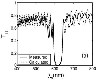
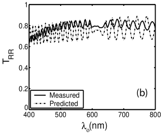
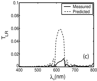
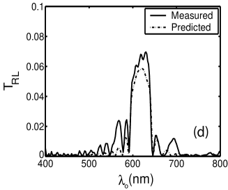
Figure 1: Computed and measured spectrums of the axial trasnmittances of a chiral STF: (a) $T_{LL}$, (b) $T_{RR}$, (c) $T_{LR}$, and (d) $T_{RL}$. Computations were carried out with $\gamma_{3}=20$, $\gamma_{2}=1.06$, $\Omega=173$nm, $L=30\Omega$, $f=0.579$, $\chi=47^{\circ}$, and $\varepsilon_{s}=6.3+0.012i$.

Sample results are presented in Figure 1. Good agreement between measured and calculated co–polarized transmittance spectrums is found over the Bragg regime which is approximately 40 nm wide. We also note that the predicted spectrums of $T_{LR}$ and $T_{RL}$ are the same [9, 21], but the measured spectrums differ. The experimentally observed difference between $T_{LR}$ and $T_{RL}$ is because the refractive index of the substrate is not the same as that of a lid covering the other face of the film. Anyhow, both cross–polarized transmittances are negligible in comparison to $T_{RR}$, and can be ignored therefore.

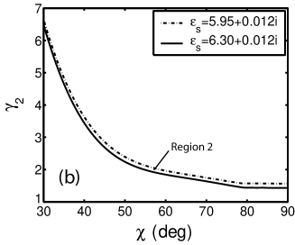
Figure 2: Regions 1 and 2 of the $\gamma_{2}-\chi$ space. The lower and upper bounds are delineated by $\varepsilon_{s}=5.95+0.012i$ (broken line) and $\varepsilon_{s}=6.30+0.012i$ (solid line).

That portion of the $\gamma_{2}$–$\chi$ space where matches between predicted and measured axial transmittances occur is presented in Figure 2. Projections of the solution regions of the $\gamma_{2}$–$\chi$–$f$ space onto the $\gamma_{2}$–$f$ and the $\chi$–$f$ planes are not shown, because we found that the value of $f$ which creates a match at the center–wavelength of the Bragg regime is nearly fixed. The center–wavelength shifts with $f$ for the measured co–polarized transmittances to be adequately matched.

The center–wavelength of the Bragg regime also shifts very slightly with variations in $\chi$, but the bandwidth of the Bragg regime depends more strongly on $\chi$. From numerous simulation trials, it appears that quite specific values of $f$ and $\gamma_{2}$ are required to match both the center–wavelength and the bandwidth of the Bragg regime, when $\chi$ is fixed.

Our model predicts two disjoint regions $\gamma_{2}$–$\chi$ space where good agreement between the model and the measurements is found. This leads, for example, to multiple values of $\chi$ corresponding to a specific value of $\gamma_{2}$. The volume fraction was found to lie in the fairly narrow range $0.51\leq f\leq 0.63$ — the lowest value corresponding to $\chi=25^{\circ}$ in Figure 2a (Region 1), and the highest value corresponding to $\chi=90^{\circ}$ in Figure 2b (Region 2).

4.3 Resolution of ambiguity

Axial transmittance data can assist in the calibration of our model, but it does leave the ambiguity between Regions 1 and 2 unresolved. The disparity between the values of $\chi$ in the two Regions is quite large. Available scanning electron micrographs do not give clear indication of $\chi$ due to shadowing effects. Furthermore, the ellipsoidal model used here is nominal, so that $\chi$ itself may only be loosely connected to the actual microstructure. We therefore examined the theoretical responses of chiral STFs to non–axial excitation by plane waves in order to resolve the ambiguity.

Let the chiral STF be excited by a plane wave propagating at an angle $\theta_{inc}$ to the $z$ axis and at an angle $\psi_{inc}$ (in the $xy$ plane) to the $x$ axis. The electric field phasor associated with the incident plane wave can be represented as [22]

$$\underline{E}_{\rm inc}(\underline{r}) = \left[\frac{\left(i\underline{s}-\underline{p}_{+}\right)}{\sqrt{2}}\,a_{\rm L}-\frac{\left(i\underline{s}+\underline{p}_{+}\right)}{\sqrt{2}}\,a_{\rm R}\right]$$ (15)

$$\qquad\times\,e^{\left[i\kappa\left(x\cos\psi_{\rm inc}+y\sin\psi_{\rm inc}\right)\right]}e^{ik_{0}z\cos\theta_{\rm inc}}\,,\,\,z\leq 0\,,$$

where

$$\kappa=k_{0}\sin\theta_{\rm inc}\,,$$ (16)

$$\underline{s}=-\underline{u}_{x}\sin\psi_{\rm inc}+\underline{u}_{y}\cos\psi_{\rm inc}\,,$$ (17)

$$\underline{p}_{\pm}=\mp\left(\underline{u}_{x}\cos\psi_{\rm inc}+\underline{u}_{y}\sin\psi_{\rm inc}\right)\cos\theta_{\rm inc}+\underline{u}_{z}\sin\theta_{\rm inc}\,.$$ (18)

The electric field phasor of the reflected plane wave can be represented as

$$\underline{E}_{\rm ref}(\underline{r}) = \left[\frac{-\left(i\underline{s}-\underline{p}_{-}\right)}{\sqrt{2}}\,r_{\rm L}+\frac{\left(i\underline{s}+\underline{p}_{-}\right)}{\sqrt{2}}\,r_{\rm R}\right]$$ (19)

$$\qquad\times\,e^{\left[i\kappa\left(x\cos\psi_{\rm inc}+y\sin\psi_{\rm inc}\right)\right]}e^{-ik_{0}z\cos\theta_{\rm inc}}\,\,,z\leq 0\,,$$

and that of the transmitted plane wave as

$$\underline{E}_{\rm tr}(\underline{r}) = \left[\frac{\left(i\underline{s}-\underline{p}_{+}\right)}{\sqrt{2}}\,t_{\rm L}-\frac{\left(i\underline{s}+\underline{p}_{+}\right)}{\sqrt{2}}\,t_{\rm R}\right]$$ (20)

$$\qquad\times\,e^{\left[i\kappa\left(x\cos\psi_{\rm inc}+y\sin\psi_{\rm inc}\right)\right]}e^{ik_{0}\left(z-L\right)\cos\theta_{\rm inc}}\,,\,\,z\geq L\,.$$

A boundary value problem similar to that for axial excitation was solved to obtain the four coefficients of (12). The angles of incidence were set at $\theta_{inc}=60^{\circ}$ and $\psi_{inc}=0^{\circ}$, while $\varepsilon_{s}=5.95+0.012i$ was chosen independent of the wavelength. The spectrums of $T_{LL}$ are presented in Figure 3 for the following three cases:

• $\gamma_{2}=1.06$, $\chi=45^{\circ}$, $f=0.592$ (Region 1),

• $\gamma_{2}=2.70$, $\chi=45^{\circ}$, $f=0.585$ (Region 2), and

• $\gamma_{2}=1.47$, $\chi=90^{\circ}$, $f=0.630$ (Region 2).

These results clearly indicate that the non–axial transmittances of chiral STFs with quite different microstructural parameters will be different from one another even though their axial transmittances are virtually indistinguishable. The Bragg phenomenon virtually disappears for Case C, but not for Cases A and B. The value of $\gamma_{2}$ can also be distinguished through non–axial transmittance measurements, as is obvious from the differences between Cases A and B in Figure 3.

5 CONCLUDING REMARKS

A chiral sculptured thin film was fabricated from Patinal titanium oxide using the serial bideposition technique, and axial transmittance spectrums were measured over a band of wavelengths encompassing the Bragg regime for axial excitation. The same transmittances were simulated using a nominal structure–property relationship model. The $\gamma_{2}$–$\chi$–$f$ parameter space was explored for best fits of the calculated transmittances to the measured values.

The following conclusions were arrived at:

• Porosity of chiral STFs was reaffirmed by our model.

• Axial transmittance data can not completely resolve ambiguities in the calibration of the model.

• Non–axial transmittance data appears crucial to the resolution of the ambiguities.

We expect to present a detailed calibration scheme in our future publications.

Figure Captions

Figure 1. Computed and measured spectrums of the axial trasnmittances of a chiral STF: (a) $T_{LL}$, (b) $T_{RR}$, (c) $T_{LR}$, and (d) $T_{RL}$. Computations were carried out with $\gamma_{3}=20$, $\gamma_{2}=1.06$, $\Omega=173$nm, $L=30\Omega$, $f=0.579$, $\chi=47^{\circ}$, and $\varepsilon_{s}=6.3+0.012i$.

Figure 2. Regions 1 and 2 of the $\gamma_{2}-\chi$ space. The lower and upper bounds are delineated by $\varepsilon_{s}=5.95+0.012i$ (broken line) and $\varepsilon_{s}=6.30+0.012i$ (solid line).

Figure 3. Calculated spectrums of $T_{LL}$ for non–axial excitation of a chiral STF. These correspond to Cases A (dot–dashed), B (dashed), and C (solid) described in Section 4.3. Computations were carried out with $\gamma_{3}=20$, $\epsilon_{s}=5.95+0.012i$, $\Omega=173$ nm, and $L=30\Omega$.

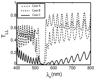
Figure 3: Calculated spectrums of $T_{LL}$ for non–axial excitation of a chiral STF. These correspond to Cases A (dot–dashed), B (dashed), and C (solid) described in Section 4.3. Computations were carried out with $\gamma_{3}=20$, $\epsilon_{s}=5.95+0.012i$, $\Omega=173$ nm, and $L=30\Omega$.

References

- [1] A. Lakhtakia, R. Messier, M. J. Brett, K. Robbie, Innovat. Mater. Res. 1 (1996) 165.
- [2] A. Lakhtakia, Mater. Sci. Engg. C 19 (2002) 427.
- [3] R. Messier, V.C. Venugopal, P.D. Sunal, J. Vac. Sci. Technol. A 18 (2000) 1538.
- [4] I. Hodgkinson, Q.h. Wu, Adv. Mater. 13 (2001) 889.
- [5] O.R. Monteiro, A. Vizir, I.G. Brown, J. Phys. D: Appl. Phys. 31 (1998) 3188.
- [6] F. Liu, M.T. Umlor, L. Shen, J. Weston, W. Eads, J.A. Barnard, G.J. Mankey, J. Appl. Phys. 85 (1999) 5486.
- [7] K.D. Harris, M.J. Brett, T.J. Smy, C. Backhouse, J. Electrochem. Soc. 147 (2000) 2002.
- [8] M. Suzuki, Y. Taga, Jpn. J. Appl. Phys. Pt. 2 40 (2001) L358.
- [9] V.C. Venugopal, A. Lakhtakia in: O.N. Singh and A. Lakhtakia (Editors), Electromagnetic fields in unconventional materials and structures, Wiley, New York, 2000 (Chapter 5).
- [10] A. Lakhtakia, M.W. McCall, J.A. Sherwin, Q. Wu, I.J. Hodgkinson, Opt. Commun. 194 (2001) 33.
- [11] I.J. Hodgkinson, Q. Wu, B. Knight, A. Lakhtakia, K. Robbie, Appl. Opt. 39 (2000) 642.
- [12] J.A. Sherwin, A. Lakhtakia, Proc. SPIE 4097 (2000) 250.
- [13] J.A. Sherwin, A. Lakhtakia, Math. Comput. Model. 34 (2001) 1499; erratums: 35 (2002) in press.
- [14] I. Hodgkinson, Q. Wu, J. Hazel, Appl. Opt. 37 (1998) 2653.
- [15] W.S. Weiglhofer, A. Lakhtakia, B. Michel, Microw. Opt. Technol. Lett. 15 (1997) 263; erratum: 22 (1999) 221.
- [16] Q. Wu, I.J. Hodgkinson, A. Lakhtakia, Opt. Engg. 39 (2000)1863.
- [17] I. J. Hodgkinson, Q. Wu, S. Collett, Appl. Opt. 40 (2001) 452.
- [18] W.L. Bragg, A.B. Pippard, Acta Crystallogr. 6 (1953) 865.
- [19] J.A. Sherwin, A. Lakhtakia, Microw. Opt. Technol. Lett. 33 (2002) 40.
- [20] http://www.emicoe.com, EM Industries Inc., Darmstadt, Germany, consulted: March 5, 2002.
- [21] M.W. McCall, Math. Comput. Model. 34 (2001) 1483.
- [22] V. C. Venugopal, A. Lakhtakia, Proc. R. Soc. Lond. A 456 (2000) 125.