Geometry of escape and transition dynamics in the presence of dissipative and gyroscopic forces in two degree of freedom systems

Abstract

Escape from a potential well can occur in different physical systems, such as capsize of ships, resonance transitions in celestial mechanics, and dynamic snap-through of arches and shells, as well as molecular reconfigurations in chemical reactions. The criteria and routes of escape in one-degree of freedom systems has been well studied theoretically with reasonable agreement with experiment. The trajectory can only transit from the hilltop of the one-dimensional potential energy surface. The situation becomes more complicated when the system has higher degrees of freedom since it has multiple routes to escape through an equilibrium of saddle-type, specifically, an index-1 saddle. This paper summarizes the geometry of escape across a saddle in some widely known physical systems with two degrees of freedom and establishes the criteria of escape providing both a methodology and results under the conceptual framework known as tube dynamics. These problems are classified into two categories based on whether the saddle projection and focus projection in the symplectic eigenspace are coupled or not when damping and/or gyroscopic effects are considered. For simplicity, only the linearized system around the saddle points is analyzed, but the results generalize to the nonlinear system. We define a transition region, $\mathcal{T}_{h}$, as the region of initial conditions of a given initial energy $h$ which transit from one side of a saddle to the other. We find that in conservative systems, the boundary of the transition region, $\partial\mathcal{T}_{h}$, is a cylinder, while in dissipative systems, $\partial\mathcal{T}_{h}$ is an ellipsoid.

1 Introduction

Transition events are very common in both the natural world, daily life and even industrial applications. Examples of transition are the snap-through of plant leaves and engineering structures responding to stimuli [1, 2], the flipping over of umbrellas on a windy day, reaction rates in chemical reaction dynamics [3], the escape and recapture of comets and spacecraft in celestial mechanics [4, 5, 6], and the capsize of ships [7, 8]. Better understanding and prediction of transitions, or escape, have significance in both utilization and evasion of such events, such as how to transfer spacecraft in specific space missions from one prescribed initial orbit to a desired final orbit with lower energy, or in structural mechanics, how to avoid collapse of structures. From the perspective of mechanics, such behavior can be interpreted as the escape from one local minimum of potential energy (i.e., a potential well) to another, which has been widely been studied as ‘escape dynamics’ [9, 10, 11, 12, 13]. Escape in a one degree of freedom system, like a double-well oscillator, is unambiguous, as the phase space is two dimensional and the hilltop equilibrium becomes a saddle point in phase space. The only way the system state can escape from the potential energy minimum is by passing over the hilltop to another local minimum. Therefore, all trajectories which have an energy above that of the hilltop, as evaluated as they pass through the location of the hilltop, transit from one side to the other. This situation has been studied by both experiments and theory with good agreement between the two [14, 15, 16].

Higher degree of freedom systems, however, are more complicated since there are multiple paths to transition through an index-1 saddle equilibrium point, as the phase space is now four dimensions or more. For such systems, it is of importance to establish systematic methods and criteria to predict the escape from a potential well. In this paper, we focus on two degrees of freedom systems, an intermediate situation, to simplify the analysis procedure, and consider the effect of damping and gyroscopic forces both in isolation and in combination. We take a Hamiltonian point of view and use canonical Hamiltonian variables, even when dissipation is included.

Generally, escape can occur only when the system has energy higher than the escape energy which is the critical energy that allows escape, the energy of the saddle point [2, 8, 11, 12]. If the energy is lower than the escape energy, the zero velocity curve (or surface)—which is the boundary of the projection of the energy manifold onto position space—is closed, allowing no open neck region around the saddle point. In this case, all of the trajectories are bounded to only evolve within their potential wells of origin and no trajectory can escape from the well. For initial conditions with energy higher than the escape energy, the equipotential surfaces open around the saddle point in a neck region, and trajectories have a chance to escape the potential well to another or even to infinity. However, the energy criterion alone is not sufficient to guarantee escape. The dynamic boundary between transition and non-transition of a system with energy higher than critical energy can be thoroughly understood under the conceptual framework of transition dynamics or sometimes known as tube dynamics [2, 8, 17, 18, 19]. In conservative two degrees of freedom systems with energy higher than the critical energy, there is an unstable periodic orbit in the bottleneck region. Emanating from the periodic orbit are its stable and unstable manifolds which have cylindrical or “tube” geometry within the conserved energy manifold. The tube manifold, sometimes called a transition tube in tube dynamics, consists of pieces of asymptotic orbits. As stated in [10], the best systematic way to study the escape from such a system is by calculating the asymptotic orbits of the periodic orbit. The reason is that the transition tube, acting like a separatrix, separates two distinct types of orbits: transit orbits and non-transit orbits. Transit orbits are those inside of the tube which can escape from one potential well to another, while non-transit, those outside of the tube, cannot pass through the bottleneck region, and thus return to their region of origin.

Although we have made it clear that the phase space structure, known as a transition tube, governs the escape in conservative systems of two degrees of freedom, it is just an ideal case since energy fluctuations and dissipation cannot be avoided in the real world. Thus, it is natural to consider how the situation will change if dissipative forces are considered. Ref. [2] has addressed this, in part, for the example of dynamic snap-through of a shallow arch. By using the bisection method, transition boundaries for both the nonlinear conservative system and dissipative system were obtained. The transition ‘tube’ for the dissipative system was found to be different from that for the conservative system. The transition tube of the conservative system not only gives all the initial conditions for transit orbits in phase space, but also gives the boundary of their evolution, while the transition ‘tube’ for the dissipative system merely gives the boundary of the initial conditions of a specific initial energy for transit orbits on a specific Poincaré section and the evolution of the transit orbits with those initial conditions is not along an invariant energy manifold any longer. As for the global structure of the phase space in the dissipative system that governs the initial conditions of transit orbits, this was not addressed in [2]. In the current study, we continue this study and answer in more detail the concern of how the situation changes when dissipation is present, finding that the transition tube in the conservative system becomes a transition ellipsoid in the dissipative system.

On the other hand, when the system is rotating or magnetic forces are present, gyroscopic forces must be considered. Gyroscopic forces, widely found in rotating systems [20, 21, 22, 23, 24] as well as electromagnetic systems, are non-dissipative and the gyroscopic coefficients enter the equations of motion in a skew-symmetric manner [20]. Some researchers have studied escape in conservative gyroscopic systems (e.g., [25, 6]). There exist transition tubes controlling the escape which are topologically the same as in an inertial system [2, 8, 26]. However, to the best knowledge of the authors, no study has been carried out to study the escape in systems with both dissipative and gyroscopic forces present. In fact, gyroscopic systems are interesting due to some unexpected phenomena which have some uncommon features. In conservative gyroscopic systems, motion near an unstable point of the potential energy surface, such as an index-1 saddle point, can be stabilized via gyroscopic forces, e.g., rotation with large enough angular velocity [23, 24, 27, 28]. But small dissipation can make the system lose the stability which is called dissipation-induced instability [22], different from the common notion that dissipation makes a system more stable. Considering this difference in dynamical behavior, another concern is whether the dynamical behavior of the dissipative system will be the same if the gyroscopic forces are included. This study will also partially answer this concern.

In this paper, we will establish criteria and present methods to estimate the transition in different physical problems with two degrees of freedom. The systems are: an idealized rolling ball on both stationary and rotating saddle surfaces, the pitch and roll dynamics of a ship near the capsize state with equal and unequal damping, the snap-through of a shallow arch, and potential well transitions in the planar circular restricted three-body problem (PCR3BP). The focus of this analysis is the local behavior near the neck region around the saddle point, obtained via the linearized dynamics. The corresponding global behavior are left for future work. In such linearized systems, the equilibrium point is of type saddle $\times$ center in the conservative system (i.e., an index-1 saddle) which becomes a saddle $\times$ focus when dissipation is considered. In other words, the equilibrium point changes from one with a one-dimensional stable, one-dimensional unstable, and two-dimensional center manifold, to one with a three-dimensional stable and one-dimensional unstable manifold. To compare the similarities and differences between the conservative and dissipative system in each setting, we introduce the same change of variables that uses the generalized eigenvectors of the corresponding conservative system, which we refer to as the symplectic eigenspace.

In the symplectic eigenspace, the dynamics in the saddle and focus projections are coupled for some dissipative systems, while for others, they remain uncoupled. Thus, this paper classifies different systems into two categories depending on the resulting linear coupling between the saddle and focus variables of the transformed dissipative system. The example problems considered share the same dynamic behavior so that we only need to give the full analysis for just one as an exemplar representative. Among the problems we will discuss, the idealized ball rolling on a saddle surface is of special interest since it can be either an inertial system or gyroscopic system, depending on whether the surface is stationary or rotating so that it can have the properties of both types of problems. Thus, we will focus on analyzing the idealized ball rolling on a surface, where the rotation is about the saddle point itself. The other examples will be shown to be equivalent to a standard form derived for the idealized ball rolling on a surface. The PCR3BP from celestial mechanics is a final special case as it involves rotation, but not about the saddle point. When a certain kind of dissipation is included, the saddle point changes location compared with the conservative system and special care needs to be taken for this case, using an effective quadratic Hamiltonian about the saddle point.

2 Transition region for the conservative case

A linear two degrees of freedom conservative system with a saddle-center type equilibrium point (i.e., index-1 or rank-1 saddle) [2, 3, 4, 5, 8] can be transformed via a canonical transformation to normal form coordinates $(q_{1},q_{2},p_{1},p_{2})$ such that the quadratic Hamiltonian, $\mathcal{H}_{2}$, can be written in the normal form,

$$\mathcal{H}_{2}=\lambda q_{1}p_{2}+\tfrac{1}{2}\omega_{p}\left(q_{2}^{2}+p_{2}^{2}\right),$$ (1)

where $q_{i}$ and $p_{i}$ are the generalized coordinates and corresponding momenta. The Hamiltonian equations are defined as

$$\dot{q}_{i}=\frac{\partial\mathcal{H}_{2}}{\partial p_{i}},\hskip 14.45377pt\dot{p}_{i}=-\frac{\partial\mathcal{H}_{2}}{\partial q_{i}},$$ (2)

which yields the following equations of motion,

$$\dot{q}_{1} =\lambda q_{1},\hskip 14.45377pt \dot{p}_{1}=-\lambda p_{1},$$ (3)

$$\dot{q}_{2} =\omega_{p}p_{2},\hskip 14.45377pt \dot{p}_{2}=-\omega_{p}q_{2},$$

where the dot over the variable denotes the derivative with respect to time. In the above equations, $\lambda$ is the real eigenvalue corresponding to the saddle coordinates spanned by $(q_{1},p_{1})$ and $\omega_{p}$ is the frequency associated with the center coordinates $(q_{2},p_{2})$. The solutions can be written as,

$$q_{1}=q_{1}^{0}e^{\lambda t},\hskip 14.45377ptp_{1}=p_{1}^{0}e^{-\lambda t},$$ (4)

$$q_{2}+ip_{2}=\left(q_{2}^{0}+ip_{2}^{0}\right)e^{-i\omega_{p}t}.$$

Note that,

$$f_{1}=q_{1}p_{1},\hskip 14.45377ptf_{2}=q_{2}^{2}+p_{2}^{2}$$ (5)

are two independent constants of motion under the Hamiltonian system (1) with $\mathcal{H}_{2}$ itself trivially a constant of motion.

2.1 Boundary of transit and non-transit orbits

The linearized phase space

For positive $h$ and $c$, the equilibrium or bottleneck region $\mathcal{R}$ (sometimes just called the neck region), which is determined by,

$$\mathcal{H}_{2}=h,\quad\mbox{and}\quad|p_{1}-q_{1}|\leq c,$$

where $c>0$, is homeomorphic to the product of a 2-sphere and an interval $I\in\mathbb{R}$, $S^{2}\times I$; namely, for each fixed value of $p_{1}-q_{1}$ in the interval $I=[-c,c]$, we see that the equation $\mathcal{H}_{2}=h$ determines a 2-sphere,

$$\tfrac{\lambda}{4}(q_{1}+p_{1})^{2}+\tfrac{1}{2}\omega_{p}(q_{2}^{2}+p_{2}^{2})=h+\tfrac{\lambda}{4}(p_{1}-q_{1})^{2}.$$ (6)

Suppose $a\in I$, then (6) can be re-written as,

$$x_{1}^{2}+q_{2}^{2}+p_{2}^{2}=r^{2},$$ (7)

where $x_{1}=\sqrt{\tfrac{1}{2}\tfrac{\lambda}{\omega_{p}}}(q_{1}+p_{1})$ and $r^{2}=\tfrac{2}{\omega_{p}}(h+\tfrac{\lambda}{4}a^{2})$, which defines a 2-sphere of radius $r$ in the three variables $x_{1}$, $q_{2}$, and $p_{2}$.

The bounding 2-sphere of $\mathcal{R}$ for which $p_{1}-q_{1}=c$ will be called $n_{1}$ (the “left” bounding 2-sphere), and where $p_{1}-q_{1}=-c$, $n_{2}$ (the “right” bounding 2-sphere). Therefore, $\partial\mathcal{R}=\{n_{1},n_{2}\}$. See Figure 1.

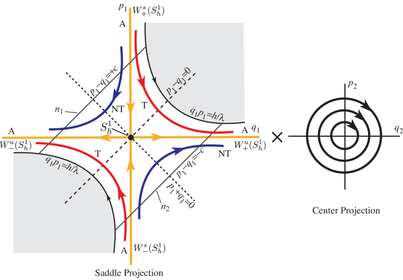
Figure 1: The flow in the equilibrium region for the conservative system has the form saddle $\times$ center. On the left is shown a schematic of the projection onto the $(q_{1},p_{1})$-plane, the saddle projection. For the conservative dynamics, the Hamiltonian function $\mathcal{H}_{2}$ remains constant at $h>0$. Shown are the periodic orbit (black dot at the center), the asymptotic orbits (labeled A), two transit orbits (T) and two non-transit orbits (NT).

We call the set of points on each bounding 2-sphere where $q_{1}+p_{1}=0$ the equator, and the sets where $q_{1}+p_{1}>0$ or $q_{1}+p_{1}<0$ will be called the northern and southern hemispheres, respectively.

The linear flow in $\mathcal{R}$

To analyze the flow in $\mathcal{R}$, consider the projections on the ($q_{1},p_{1}$)-plane and the $(q_{2},p_{2})$-plane, respectively. In the first case we see the standard picture of a saddle point in two dimensions, and in the second, of a center consisting of harmonic oscillator motion. Figure 1 schematically illustrates the flow. With regard to the first projection we see that $\mathcal{R}$ itself projects to a set bounded on two sides by the hyperbolas $q_{1}p_{1}=h/\lambda$ (corresponding to $q_{2}^{2}+p_{2}^{2}=0$, see (1)) and on two other sides by the line segments $p_{1}-q_{1}=\pm c$, which correspond to the bounding 2-spheres, $n_{1}$ and $n_{2}$, respectively.

Since $q_{1}p_{1}$ is an integral of the equations in $\mathcal{R}$, the projections of orbits in the $(q_{1},p_{1})$-plane move on the branches of the corresponding hyperbolas $q_{1}p_{1}=$ constant, except in the case $q_{1}p_{1}=0$, where $q_{1}=0$ or $p_{1}=0$. If $q_{1}p_{1}>0$, the branches connect the bounding line segments $p_{1}-q_{1}=\pm c$ and if $q_{1}p_{1}<0$, they have both end points on the same segment. A check of equation (4) shows that the orbits move as indicated by the arrows in Figure 1.

To interpret Figure 1 as a flow in $\mathcal{R}$, notice that each point in the $(q_{1},p_{1})$-plane projection corresponds to a 1-sphere, $S^{1}$, or circle, in $\mathcal{R}$ given by,

$$q_{2}^{2}+p_{2}^{2}=\tfrac{2}{\omega_{p}}(h-\lambda q_{1}p_{1}).$$

Of course, for points on the bounding hyperbolic segments ($q_{1}p_{1}=h/\lambda$), the 1-sphere collapses to a point. Thus, the segments of the lines $p_{1}-q_{1}=\pm c$ in the projection correspond to the 2-spheres bounding $\mathcal{R}$. This is because each corresponds to a 1-sphere crossed with an interval where the two end 1-spheres are pinched to a point.

We distinguish nine classes of orbits grouped into the following four categories:

1. The point $q_{1}=p_{1}=0$ corresponds to an invariant 1-sphere $S^{1}_{h}$, an unstable periodic orbit in $\mathcal{R}$ of energy $\mathcal{H}_{2}=h$. This 1-sphere is given by,

   $$q_{2}^{2}+p_{2}^{2}=\tfrac{2}{\omega_{p}}h,\hskip 21.68121ptq_{1}=p_{1}=0.$$ (8)

   It is an example of a normally hyperbolic invariant manifold (NHIM) (see [29]). Roughly, this means that the stretching and contraction rates under the linearized dynamics transverse to the 1-sphere dominate those tangent to the 1-sphere. This is clear for this example since the dynamics normal to the 1-sphere are described by the exponential contraction and expansion of the saddle point dynamics. Here the 1-sphere acts as a “big saddle point”. See the black dot at the center of the $(q_{1},p_{1})$-plane on the left side of Figure 1.

2. The four half open segments on the axes, $q_{1}p_{1}=0$, correspond to four cylinder surfaces of orbits asymptotic to this invariant 1-sphere $S^{1}_{h}$ either as time increases ($q_{1}=0$) or as time decreases ($p_{1}=0$). These are called asymptotic orbits and they are the stable and the unstable manifolds of $S^{1}_{h}$. The stable manifolds, $W^{s}_{\pm}(S^{1}_{h})$, are given by,

   $$q_{2}^{2}+p_{2}^{2}=\tfrac{2}{\omega_{p}}h,\hskip 21.68121ptq_{1}=0,\hskip 21.68121ptp_{1}~{}{\rm arbitrary}.$$ (9)

   $W^{s}_{+}(S^{1}_{h})$ (with $p_{1}>0$) is the branch entering from $n_{1}$ and $W^{s}_{-}(S^{1}_{h})$ (with $p_{1}<0$) is the branch entering from $n_{2}$. The unstable manifolds, $W^{u}_{\pm}(S^{1}_{h})$, are given by,

   $$q_{2}^{2}+p_{2}^{2}=\tfrac{2}{\omega_{p}}h,\hskip 21.68121ptp_{1}=0,\hskip 21.68121ptq_{1}~{}{\rm arbitrary}$$ (10)

   $W^{u}_{+}(S^{1}_{h})$ (with $q_{1}>0$) is the branch exiting from $n_{2}$ and $W^{u}_{-}(S^{1}_{h})$ (with $q_{1}<0$) is the branch exiting from $n_{1}$. See the four orbits labeled A of Figure 1.

3. The hyperbolic segments determined by $q_{1}p_{1}={\rm constant}>0$ correspond to two solid cylinders of orbits which cross $\mathcal{R}$ from one bounding 2-sphere to the other, meeting both in the same hemisphere; the northern hemisphere if they go from $p_{1}-q_{1}=+c$ to $p_{1}-q_{1}=-c$, and the southern hemisphere in the other case. Since these orbits transit from one realm to another, we call them transit orbits. See the two orbits labeled T of Figure 1.

4. Finally the hyperbolic segments determined by $q_{1}p_{1}={\rm constant}<0$ correspond to two cylinders of orbits in $\mathcal{R}$ each of which runs from one hemisphere to the other hemisphere on the same bounding 2-sphere. Thus if $q_{1}>0$, the 2-sphere is $n_{2}$ ($p_{1}-q_{1}=-c$) and orbits run from the southern hemisphere ($q_{1}+p_{1}<0$) to the northern hemisphere ($q_{1}+p_{1}>0$) while the converse holds if $q_{1}<0$, where the 2-sphere is $n_{1}$. Since these orbits return to the same realm, we call them non-transit orbits. See the two orbits labeled NT of Figure 1.

We define the transition region, $\mathcal{T}_{h}$, as the region of initial conditions of a given initial energy $h$ which transit from one side of the neck region to the other. This is the set of all transit orbits, which has the geometry of a solid cylinder. The transition region, $\mathcal{T}_{h}$, is made up of one half which goes to the right (from $n_{1}$ to $n_{2}$), $\mathcal{T}_{h+}$, defined by $q_{1}p_{1}={\rm constant}>0$ with both $q_{1}>0$ and $p_{1}>0$, and the other half which goes to the left (from $n_{2}$ to $n_{1}$), $\mathcal{T}_{h-}$, defined by $q_{1}p_{1}={\rm constant}>0$ with both $q_{1}<0$ and $p_{1}<0$. The boundaries are $\partial\mathcal{T}_{h+}$ and $\partial\mathcal{T}_{h-}$, respectively. The closure of $\partial\mathcal{T}_{h}$, $\overline{\partial\mathcal{T}_{h}}$, is equal to the boundaries $\partial\mathcal{T}_{h+}$ and $\partial\mathcal{T}_{h-}$, along with the periodic orbit $S^{1}_{h}$, i.e., $\partial\mathcal{T}_{h-}\cup\partial\mathcal{T}_{h+}\cup S^{1}_{h}$.

In summary, for the conservative case, the boundary of the transition region, $\partial\mathcal{T}_{h}$, has the topology of a cylinder. The topology of $\partial\mathcal{T}_{h}$ will be different for the dissipative case, as will be shown in later sections. For convenience, we may refer to $\partial\mathcal{T}_{h}$ and $\overline{\partial\mathcal{T}_{h}}$ interchangeably.

2.2 McGehee representation of the equilibrium region

McGehee [30], building on the work of Conley [31], proposed a representation which makes it easier to visualize the region $\mathcal{R}$. Recall that $\mathcal{R}$ is a 3-dimensional manifold that is homeomorphic to $S^{2}\times I$. In [30], it is represented by a spherical annulus bounded by the two 2-spheres $n_{1},n_{2}$, as shown in Figure 2(c).

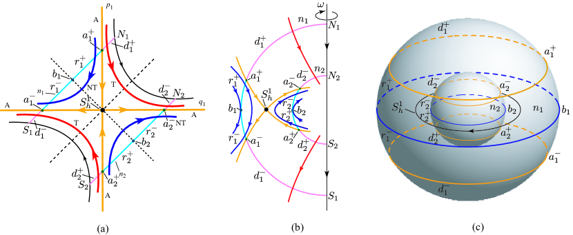
Figure 2: (a) The projection onto the $(q_{1},p_{1})$-plane, the saddle projection, with labels consistent with the text and (b) and (c). (b) The cross-section of the flow in the $\mathcal{R}$ region of the energy surface. The north and south poles of bounding sphere $n_{i}$ are labeled as $N_{i}$ and $S_{i}$, respectively. (c) The McGehee representation of the flow on the boundaries of the $\mathcal{R}$ region, highlighting the features on the bounding spheres $n_{1}$ and $n_{2}$ for $h>0$.

Figure 2(a) is a cross-section of $\mathcal{R}$. Notice that this cross-section is qualitatively the same as the saddle projection illustration in Figure 1. The full picture (Figure 2(c)) is obtained by rotating this cross section, Figure 2(b), about the indicated axis, where the azimuthal angle $\omega$ roughly describes the angle in the center projection in Figure 1. The following classifications of orbits correspond to the previous four categories:

1. There is an invariant 1-sphere $S^{1}_{h}$, a periodic orbit in the region $\mathcal{R}$ corresponding to the black dot in the middle of Figure 2(a). Notice that this 1-sphere is the equator of the central 2-sphere given by $p_{1}-q_{1}=0$.

2. Again let $n_{1},n_{2}$ be the bounding 2-spheres of region $\mathcal{R}$, and let $n$ denote either $n_{1}$ or $n_{2}$. We can divide $n$ into two hemispheres: $n^{+}$, where the flow enters $\mathcal{R}$, and $n^{-}$, where the flow leaves $\mathcal{R}$. There are four cylinders of orbits asymptotic to the invariant 1-sphere $S^{1}_{h}$. They form the stable and unstable manifolds which are asymptotic to the invariant 1-sphere $S^{1}_{h}$. Topologically, both invariant manifolds look like 2-dimensional cylinders or “tubes” ($S^{1}\times{\mathbb{R}}$) inside a 3-dimensional energy manifold. The interior of the stable manifolds $W^{s}_{\pm}(S^{1}_{h})$ and unstable manifolds $W^{u}_{\pm}(S^{1}_{h})$ can be given as follows

   $$\begin{split}{\rm int}(W^{s}_{+}(S^{1}_{h}))&=\{(q_{1},p_{1},q_{2},p_{2})\in\mathcal{R}\mid\hskip 7.22743ptp_{1}>q_{1}>0\},\\ {\rm int}(W^{s}_{-}(S^{1}_{h}))&=\{(q_{1},p_{1},q_{2},p_{2})\in\mathcal{R}\mid\hskip 7.22743ptp_{1}<q_{1}<0\},\\ {\rm int}(W^{u}_{+}(S^{1}_{h}))&=\{(q_{1},p_{1},q_{2},p_{2})\in\mathcal{R}\mid\hskip 7.22743ptq_{1}>p_{1}>0\},\\ {\rm int}(W^{u}_{-}(S^{1}_{h}))&=\{(q_{1},p_{1},q_{2},p_{2})\in\mathcal{R}\mid\hskip 7.22743ptq_{1}<p_{1}<0\}.\end{split}$$ (11)

   The exterior of these invariant manifolds can be given similarly from studying Figure 2(a) and (b).

3. Let $a^{+}$ and $a^{-}$ (where $q_{1}=0$ and $p_{1}=0$ respectively) be the intersections of the stable and unstable manifolds with the bounding sphere $n$. Then $a^{+}$ appears as a 1-sphere in $n^{+}$, and $a^{-}$ appears as a 1-sphere in $n^{-}$. Consider the two spherical caps on each bounding 2-sphere given by

   $$d_{1}^{+} =\{(q_{1},p_{1},q_{2},p_{2})\in\mathcal{R}\mid\hskip 7.22743ptp_{1}-q_{1}=+c,\hskip 7.22743ptp_{1}>q_{1}>0\},$$

   $$d_{1}^{-} =\{(q_{1},p_{1},q_{2},p_{2})\in\mathcal{R}\mid\hskip 7.22743ptp_{1}-q_{1}=+c,\hskip 7.22743ptq_{1}<p_{1}<0\},$$

   $$d_{2}^{+} =\{(q_{1},p_{1},q_{2},p_{2})\in\mathcal{R}\mid\hskip 7.22743ptp_{1}-q_{1}=-c,\hskip 7.22743ptp_{1}<q_{1}<0\},$$

   $$d_{2}^{-} =\{(q_{1},p_{1},q_{2},p_{2})\in\mathcal{R}\mid\hskip 7.22743ptp_{1}-q_{1}=-c,\hskip 7.22743ptq_{1}>p_{1}>0\}.$$

   Since $d_{1}^{+}$ is the spherical cap in $n_{1}^{+}$ bounded by $a_{1}^{+}$, then the transit orbits entering $\mathcal{R}$ on $d_{1}^{+}$ exit on $d_{2}^{-}$ of the other bounding sphere. Similarly, since $d_{1}^{-}$ is the spherical cap in $n_{1}^{-}$ bounded by $a_{1}^{-}$, the transit orbits leaving on $d_{1}^{-}$ have come from $d_{2}^{+}$ on the other bounding sphere. Note that all spherical caps where the transit orbits pass through are in the interior of stable and unstable manifold tubes.

4. Let $b$ be the intersection of $n^{+}$ and $n^{-}$ (where $q_{1}+p_{1}=0$). Then, $b$ is a 1-sphere of tangency points. Orbits tangent at this 1-sphere “bounce off,” i.e., do not enter $\mathcal{R}$ locally. Moreover, if we let $r^{+}$ be a spherical zone which is bounded by $a^{+}$ and $b$, then non-transit orbits entering $\mathcal{R}$ on $r^{+}$ exit on the same bounding 2-sphere through $r^{-}$ which is bounded by $a^{-}$ and $b$. It is easy to show that all the spherical zones where non-transit orbits bounce off are in the exterior of stable and unstable manifold tubes.

The McGehee representation provides an additional, perhaps clearer, visualization of the dynamics in the equilibrium region. In particular, the features on the two spheres, $n_{1}$ and $n_{2}$, which form $\partial\mathcal{R}$ for a constant $h>0$, can be considered in the dissipative case as well, and compared with the situation in the conservative case, as shown for some examples below. The spheres $n_{1}$ and $n_{2}$ can be considered as spherical Poincaré sections parametrized by their distance from the saddle point, $c$, which reveal the topology of the transition region boundary, $\partial\mathcal{T}_{h}$, particularly through how the geometry of $a_{i}^{+}$ and $a_{i}^{-}$ (for $i=1,2$) change as $c$ changes.

3 Uncoupled systems in the dissipative case

As pointed out in the introduction, when applying the symplectic change of variables consisting of the generalized eigenvectors of the conservative system to the dissipative system, the saddle projection and focus projection are coupled in some systems, while in others systems they are not. According to the coupling conditions, the systems are classified into two categories: uncoupled systems and coupled systems. In this section, we will discuss the uncoupled systems first.

3.1 Ball rolling on a stationary surface

Among the examples of escape from potential wells, a small ball or particle moving in an idealized fashion on a surface is an easy one from the perspective of both theory and experiment. The tracking of the moving object is easily executed by using a high-speed digital camera which is much easier than measurements of structural snap-through or ship motion, not to mention the motion of spacecraft in space. It can be either an inertial system or a gyroscopic system depending on whether the surface is stationary or rotating, due to a turntable, for instance [32]. The easy switch between non-gyroscopic system and gyroscopic system makes it easy to compare their similarities and differences in escape from potential wells. The mathematical model of a rolling ball on a stationary surface was established in [33]. Experiments [26, 34] regarding escape from the potential wells on similar surfaces were shown to validate the theory of the phase space conduits predicted by the mathematical model, which mediate the transitions between wells in the system. The dissipation of energy cannot be avoided in any physical experiment, but over small enough time-scales of interest, [26] justified that dissipation could be ignored. The good agreement between the theory and experiment to within $1\%$ indicates the robustness of the transition tube in the conservative systems. However, it is still not clear how dissipation affects the transition of a rolling ball on a surface and what the phase space structure controlling the transition in the corresponding dissipative system is. In the current example, we will present the answers.

3.1.1 Governing equations

Here we consider a ball with unit mass rolling on a surface without slipping. Before analyzing the dynamical behavior of the rolling ball, a Cartesian coordinate system $o\mbox{-}xyz$ with $z$ oriented upward is established. Thus, the equations of the surface can be determined by $z=H(x,y)$. In the current study, a saddle surface of the following form is selected,

$$H(x,y)=\tfrac{1}{2}\left(k_{1}x^{2}+k_{2}y^{2}\right),\hskip 21.68121ptk_{1}=-5.91~{}\text{m}^{-1},k_{2}=3.94~{}\text{m}^{-1},$$ (12)

which is shown in Figure 3.

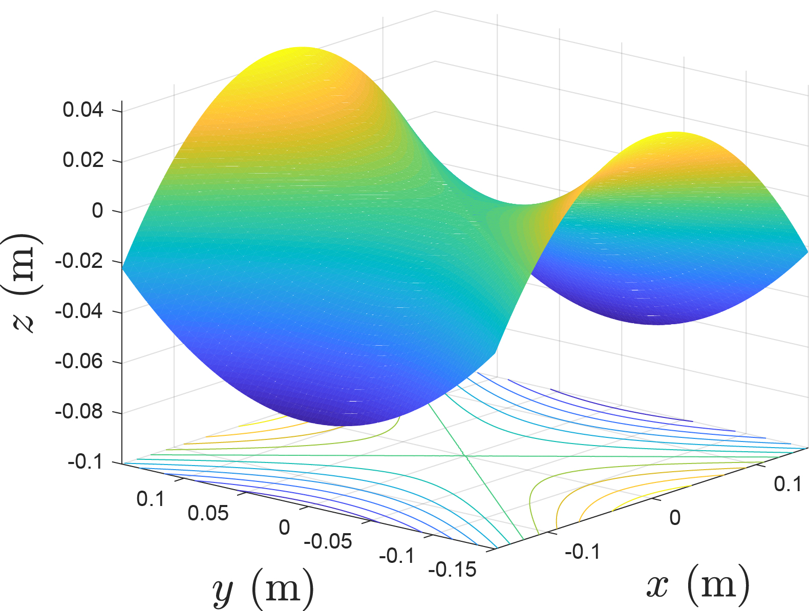
Figure 3: The graph of the example saddle surface considered, based on (12). The contours of the surface are projected on the bottom plane. The $z$ direction is shown scaled by a factor of 2 compared to $x$ and $y$ in order to highlight the saddle nature of the surface.

Before analyzing the dynamical behavior of the system, one needs to obtain the equations of motion. To do so, one can use either the Lagrangian approach or Hamiltonian approach [20]. In the Lagrangian approach, the kinetic energy and potential energy are needed to get the Lagrangian function which will yield the Euler-Lagrangian equations. In the Hamiltonian approach, the generalized momenta should be defined by introducing a Legendre transformation from the Lagrangian and then the Hamiltonian function can be given which will generate the Hamilton’s equations. In Section 4.1, we will consider a more complicated system where the surface is not stationary, but it is rotating with a constant angular velocity $\omega$ where the gyroscopic force is included. Since the stationary surface is just a special case of the rotating surface where one takes angular velocity as zero, we do not separately derive the governing equations for the stationary surface and rotating surface. The derivation of the equations of motion will be briefly described for the current problem and readers can refer to Section 4.1 for more details.

From the analysis in Section 4.1, one can set the angular velocity of the rotating surface as zero to obtain the kinetic energy (the translational plus rotational without slipping), $\mathcal{K}=\frac{1}{2}I\left(\dot{x}^{2}+\dot{y}^{2}+\dot{z}^{2}\right)$, and potential energy, $\mathcal{U}=gz$, where $g=9.81\mathrm{m/s^{2}}$ is the gravitational acceleration and $z$ and $\dot{z}$ are written in terms of $x$, $y$, $\dot{x}$ and $\dot{y}$ via the relationship $z=H(x,y)$. The factor $I=7/5$ is introduced by including rotational kinetic energy for a ball rolling without slipping. See details in the supplemental material in [26]. If we consider a particle sliding on the surface, we have $I=1$. The kinetic energy $\mathcal{K}$ and potential energy $\mathcal{U}$ are,

$$\begin{split}\mathcal{K}(x,y)&=\tfrac{1}{2}I\left[\dot{x}^{2}+\dot{y}^{2}+\left(H_{,x}\dot{x}+H_{,y}\dot{y}\right)^{2}\right],\\ \mathcal{U}(x,y)&=gH(x,y).\end{split}$$ (13)

where $H_{,x}=\partial H/\partial x$ and $H_{,y}=\partial H/\partial y$. Thus, one can define the Lagrangian function by,

$$\mathcal{L}\left(x,y\right)=\mathcal{K}\left(x,y,\dot{x},\dot{y}\right)-\mathcal{U}(x,y),$$ (14)

which generates the Euler-Lagrange equations,

$$\frac{\mathrm{d}}{\mathrm{d}t}\left(\frac{\partial\mathcal{L}}{\partial\dot{q}_{i}}\right)-\frac{\partial\mathcal{L}}{\partial q_{i}}=Q_{i},$$ (15)

where $q_{i}$ are the generalized coordinates $(x,y)$ and $Q_{i}$ are the non-conservative forces. In the current problem, a small linear viscous damping, proportional to the magnitude of the inertial velocity, is considered, with the form given via a Rayleigh dissipation function as,

$$\begin{split}Q_{x}&=-c_{d}\left[\left(1+H_{,x}^{2}\right)\dot{x}+H_{,x}H_{,y}\dot{y}\right],\\ Q_{y}&=-c_{d}\left[\left(1+H_{,y}^{2}\right)\dot{y}+H_{,x}H_{,y}\dot{x}\right],\end{split}$$ (16)

where $c_{d}$ is the coefficient of damping. The equations of motion for the current problem are,

$$I\left(1+k_{1}^{2}x^{2}\right)\ddot{x}+Ik_{1}k_{2}xy\ddot{y}+Ik_{1}^{2}x\dot{x}^{2}+Ik_{1}k_{2}x\dot{y}^{2}+gk_{1}x+c_{d}\left[\left(1+k_{1}^{2}x^{2}\right)\dot{x}+k_{1}k_{2}xy\dot{y}\right]=0,$$ (17)

$$Ik_{1}k_{2}xy\ddot{x}+I\left(1+k_{2}^{2}y^{2}\right)\ddot{y}+Ik_{1}k_{2}y\dot{x}^{2}+Ik_{2}^{2}y\dot{y}^{2}+gk_{2}y+c_{d}\left[\left(1+k_{2}^{2}y^{2}\right)\dot{y}+k_{1}k_{2}xy\dot{x}\right]=0.$$

Once the Lagrangian system is established, one can transform it to a Hamiltonian system by use of the Legendre transformation,

$$p_{i}=\frac{\partial\mathcal{L}}{\partial\dot{q}_{i}},\hskip 36.135pt\mathcal{H}\left(q_{i},p_{i}\right)=\sum_{i=1}^{n}p_{i}\dot{q}_{i}-\mathcal{L}\left(q_{i},p_{i}\right),$$ (18)

where $p_{i}$ are called the generalized momenta conjugate to the generalized coordinates $q_{i}$ and $\mathcal{H}$ the Hamiltonian function. In the current case, the Legendre transformation is given by,

$$\begin{split}p_{x}&=\frac{\partial\mathcal{L}}{\partial\dot{x}}=\dot{x}-y\omega+H_{,x}^{2}\dot{x}+H_{,x}H_{,y}\dot{y},\\ p_{y}&=\frac{\partial\mathcal{L}}{\partial\dot{y}}=\dot{y}+x\omega+H_{,x}H_{,y}\dot{x}+H_{,y}^{2}\dot{y}.\end{split}$$ (19)

Therefore, one obtains the Hamiltonian function,

$$\begin{split}\mathcal{H}=\frac{\left[p_{x}^{2}\left(1+H_{,y}^{2}\right)-2p_{x}p_{y}H_{,x}H_{,y}+p_{y}^{2}\left(1+H_{,x}^{2}\right)\right]}{2I\left(1+H_{,x}^{2}+H_{,y}^{2}\right)}+gH,\end{split}$$ (20)

where $p_{x}$ and $p_{y}$ are the momenta conjugate to $x$ and $y$, respectively. The comma in the subscript means the partial derivative with respect to the following coordinate. The general form of the Hamilton’s equations with damping [20] are given by,

$$\dot{q}_{i}=\frac{\partial\mathcal{H}}{\partial p_{i}},\hskip 36.135pt\dot{p}_{i}=-\frac{\partial\mathcal{H}}{\partial q_{i}}+Q_{i}.$$ (21)

where $Q_{i}$ is the same non-conservative generalized force written in terms of $(q,p)$ variables. For simplicity, the specific form of Hamilton’s equations for the current problem are not listed here.

For the surface adopted in (12), it has a saddle type equilibrium point at the origin $\left(0,0\right)$. To study the transition from one side of the bottleneck to the other, the local dynamical behavior near the equilibrium point plays a critical role. Thus, we will obtain the linearized Hamiltonian equations around the equilibrium point to study the local properties. A short computation for (21) gives the linearized equations of motion in Hamiltonian form as,

$$\begin{split}\dot{x}&=p_{x}/I,\\ \dot{y}&=p_{y}/I,\\ \dot{p}_{x}&=-gk_{1}x-c_{d}p_{x}/I,\\ \dot{p}_{y}&=-gk_{2}y-c_{d}p_{y}/I.\end{split}$$ (22)

We introduce the following re-scaled parameters,

$$\begin{split}\left(\bar{q}_{1},\bar{q}_{2}\right)=\left(x,y\right),\left(\bar{p}_{1},\bar{p}_{2}\right)=\left(p_{x},p_{y}\right)/I,\left(c_{x},c_{y}\right)=-g\left(k_{1},k_{2}\right)/I,c_{h}=c_{d}/I,\end{split}$$ (23)

and the equations of motion can be rewritten in the simpler re-scaled form,

$$\begin{split}\dot{\bar{q}}_{1}&=\bar{p}_{1},\\ \dot{\bar{q}}_{2}&=\bar{p}_{2},\\ \dot{\bar{p}}_{1}&=c_{x}\bar{q}_{1}-c_{h}\bar{p}_{1},\\ \dot{\bar{p}}_{2}&=c_{y}\bar{q}_{2}-c_{h}\bar{p}_{2}.\end{split}$$ (24)

Written in matrix form, with column vector $\bar{z}=\left(\bar{q}_{1},\bar{q}_{2},\bar{p}_{1},\bar{p}_{2}\right)^{T}$, we have $\dot{\bar{z}}=A\bar{z}$, where $A=M+D$, i.e.,

$$\dot{\bar{z}}=M\bar{z}+D\bar{z},$$ (25)

where,

$$M=\begin{pmatrix}0&0&1&0\\ 0&0&0&1\\ c_{x}&0&0&0\\ 0&c_{y}&0&0\end{pmatrix},\hskip 7.22743ptD=c_{h}\begin{pmatrix}0&0&0&0\\ 0&0&0&0\\ 0&0&-1&0\\ 0&0&0&-1\end{pmatrix}.$$ (26)

The corresponding quadratic Hamiltonian for the linearized system is,

$$\mathcal{H}_{2}(\bar{q}_{1},\bar{q}_{2},\bar{p}_{1},\bar{p}_{2})=\tfrac{1}{2}\left(\bar{p}_{1}^{2}+\bar{p}_{2}^{2}\right)-\tfrac{1}{2}\left(c_{x}\bar{q}_{1}^{2}+c_{y}\bar{q}_{2}^{2}\right).$$ (27)

3.1.2 Analysis in the conservative system

First we analyze the behavior in the conservative system which can be obtained by taking zero damping, $c_{h}=0$. It is straightforward to obtain the eigenvalues of the conservative system which are of the form $\pm\lambda$ and $\pm i\omega_{p}$ as expected, since the linearization matrix $A=M$ is an infinitesimal symplectic matrix (also known as a Hamiltonian matrix) [35, 36] where $\lambda$ and $\omega_{p}$ are positive constants given by $\lambda=\sqrt{c_{x}}$ and $\omega_{p}=\sqrt{-c_{y}}$. The corresponding eigenvectors are defined as $u_{\pm\lambda}$ and $u_{\omega_{p}}\pm iv_{\omega_{p}}$, where $u_{\pm\lambda}$, $u_{\omega_{p}}$, and $v_{\omega_{p}}$ are real vectors with the following form,

$$\begin{split}u_{+\lambda}&=\left(\lambda^{2}-c_{y},0,\lambda^{3}-\lambda c_{y},0\right),\\ u_{-\lambda}&=\left(-\lambda^{2}+c_{y},0,\lambda^{3}-\lambda c_{y},0\right),\\ u_{\omega_{p}}&=\left(0,\omega_{p}^{2}+c_{x},0,0\right),\\ v_{\omega_{p}}&=\left(0,0,0,\omega_{p}^{3}+\omega_{p}c_{x}\right).\end{split}$$ (28)

Considering the change of variables defined by,

$$\bar{z}=Cz,$$ (29)

where $\bar{z}=\left(\bar{q}_{1},\bar{q}_{2},\bar{p}_{1},\bar{p}_{2}\right)^{T}$ and $z=\left(q_{1},q_{2},p_{1},p_{2}\right)^{T}$, with $C=\left(u_{\lambda},u_{\omega_{p}},u_{-\lambda},v_{\omega_{p}}\right)$ where $u_{\lambda}$, etc, are understood as column vectors, one can find,

$$C^{T}JC=\begin{pmatrix}0&\bar{D}\\ -\bar{D}&0\end{pmatrix},\hskip 14.45377pt\bar{D}=\begin{pmatrix}d_{\lambda}&0\\ 0&d_{\omega_{p}}\end{pmatrix},$$

where,

$$\begin{split}d_{\lambda}&=2\lambda\left[(c_{x}-c_{y})\lambda^{2}-c_{x}c_{y}+c_{y}^{2}\right],\\ d_{\omega_{p}}&=\omega_{p}\left[(c_{x}-c_{y})\omega_{p}^{2}+c_{x}^{2}-c_{x}c_{y}\right],\end{split}$$

and $J$ is the $4\times 4$ canonical symplectic matrix,

$$J=\begin{pmatrix}0&I_{2}\\ -I_{2}&0\end{pmatrix},$$ (30)

where $I_{2}$ is the $2\times 2$ identity matrix.

We can introduce two factors $s_{1}=\sqrt{d_{\lambda}}$ and $s_{2}=\sqrt{d_{\omega_{p}}}$ to the columns in $C$ which makes it a symplectic matrix, i.e., satisfying $C^{T}JC=J$. The final form of the symplectic matrix is,

$$C=\begin{pmatrix}\tfrac{\lambda^{2}-c_{y}}{s_{1}}&0&\tfrac{-\lambda^{2}+c_{y}}{s_{1}}&0\\ 0&\tfrac{\omega_{p}^{2}+c_{x}}{s_{2}}&0&0\\ \tfrac{\lambda^{3}-\lambda c_{y}}{s_{1}}&0&\tfrac{\lambda^{3}-\lambda c_{y}}{s_{1}}&0\\ 0&0&0&\tfrac{\omega_{p}^{3}+\omega_{p}c_{x}}{s_{2}}\end{pmatrix}.$$ (31)

The equations of motion in the symplectic eigenspace (i.e., the $z$ variables) can be obtained as,

$$\dot{z}=\Lambda z,$$ (32)

where $\Lambda=C^{-1}MC$ is the conservative part of the dynamics,

$$\Lambda=\begin{pmatrix}\lambda&0&0&0\\ 0&0&0&\omega_{p}\\ 0&0&-\lambda&0\\ 0&-\omega_{p}&0&0\end{pmatrix}.$$ (33)

Thus, via the transformation (29), the equations of motion in the conservative system can be rewritten in a normal form given in (3) with Hamiltonian (1) whose solutions are given by (4).

Behavior in the position space

Recalling the solutions in (4) and the symplectic matrix $C$ in (31), we obtain the general (real) solutions of the conservative system in phase space in the form,

$$\bar{z}(t) =\left(\bar{q}_{1},\bar{q}_{2},\bar{p}_{1},\bar{p}_{2}\right)^{T}$$ (34)

$$=q_{1}^{0}e^{\lambda t}u_{+\lambda}+p_{1}^{0}e^{-\lambda t}u_{-\lambda}+\mathrm{Re}\left[\beta_{0}e^{-i\omega_{p}t}\left(u_{\omega_{p}}-iv_{\omega_{p}}\right)\right],$$

where $q_{1}^{0}$, $p_{1}^{0}$, $q_{2}^{0}$, $p_{2}^{0}$ are real and determined by initial conditions, where $\beta_{0}=q_{2}^{0}+ip_{2}^{0}$. In particular, we have,

$$\bar{q}_{1}(t) =\frac{\lambda^{2}-c_{y}}{s_{1}}q_{1}^{0}e^{\lambda t}-\frac{\lambda^{2}-c_{y}}{s_{1}}p_{1}^{0}e^{-\lambda t},$$ (35)

$$\bar{q}_{2}(t) =\frac{\omega_{p}^{2}+c_{x}}{s_{2}}\left(q_{2}^{0}\cos\omega_{p}t+p_{2}^{0}\sin\omega_{p}t\right).$$

Notice that all trajectories in the configuration space in $\mathcal{R}$ must evolve within the energy manifold which is bounded by the zero velocity curve (corresponding to $\bar{p}_{1}=\bar{p}_{2}=0$) [2, 5, 11, 12] given by solving (27) as,

$$\bar{q}_{2}=\pm\sqrt{\frac{-2h-c_{x}\bar{q}_{1}^{2}}{c_{y}}}.$$ (36)

By examining the general solution, we can see the solutions on the energy surface fall into different classes depending upon the limiting behavior of $\bar{q}_{1}$ as $t$ goes to plus or minus infinity according to the fact that $\bar{q}_{1}(t)$ is dominated by the $q_{1}^{0}$ and $p_{1}^{0}$ terms when $t\rightarrow+\infty$ and $t\rightarrow-\infty$, respectively. Thus, the nine classes of orbits determined by varying the signs of $q_{1}^{0}$ and $p_{1}^{0}$ are classified into four categories.

1. If $q_{1}^{0}=p_{1}^{0}=0$, we obtain a periodic solution with energy $h$. The periodic orbit, $S^{1}_{h}$, projects onto the $\left(\bar{q}_{1},\bar{q}_{2}\right)$ plane as a segment with length $\sqrt{-2h/c_{y}}$.

2. Orbits with $q_{1}^{0}p_{1}^{0}=0$ are asymptotic orbits. They are asymptotic to the periodic orbit, which is the origin, labeled $S_{h}^{1}$ in Figure 1. Asymptotic orbits with either $q_{1}^{0}=0$ or $p_{1}^{0}=0$ project into a strip $S$, as shown in Figure 4, bounded by lines,

   $$\bar{q}_{2}=\pm\frac{\omega_{p}^{2}+c_{x}}{s_{2}}\sqrt{\frac{2h}{\omega_{p}}}.$$ (37)

3. Orbits with $q_{1}^{0}p_{1}^{0}>0$ are transit orbits because they cross the equilibrium region $\mathcal{R}$ from $-\infty$ (the left-hand side) to $+\infty$ (the right-hand side) or vice versa.

4. Orbits with $q_{1}^{0}p_{1}^{0}<0$ are non-transit orbits.

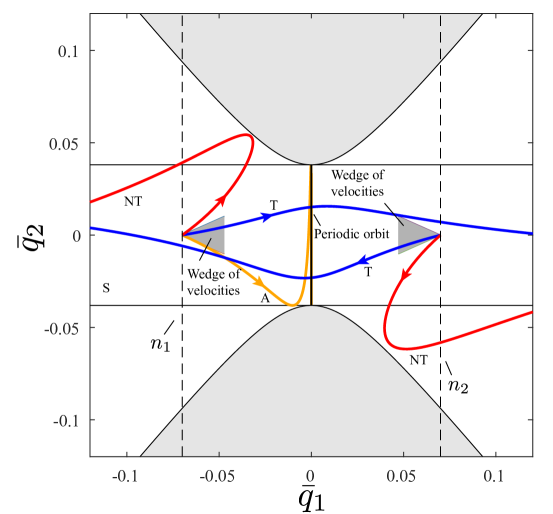
Figure 4: The flow in the equilibrium region $\mathcal{R}$ projected onto position space $(\bar{q}_{1},\bar{q}_{2})$ in the conservative system with fixed positive energy, $\mathcal{H}_{2}=h>0$, for a ball rolling on a stationary surface. Shown are the unstable periodic orbit (vertical segment in the center), a typical asymptotic orbit winding onto the the periodic orbit; two transit orbits (blue); and two non-transit orbits (red). At each point on the bounding lines $n_{1}$ or $n_{2}$ (dashed) inside the strip $S$, there is a wedge of velocity dividing different types of orbits, inside of which are transit orbits, and outside of which are non-transit orbits; specifically, the trajectories with initial conditions on the boundary are the orbits asymptotic to the unstable periodic orbit. See the text for the explanation of the details.

Figure 4 gives the four categories of orbits mentioned above. In the figure, $S$ is the strip confining the asymptotic orbits. Outside of the strip, the situation is simple and only non-transit orbits exist which means the signs of $q_{1}^{0}$ and $p_{1}^{0}$ are independent of the direction of the velocity and we always have $q_{1}^{0}p_{1}^{0}<0$. The signs in each component of the equilibrium region $\mathcal{R}$ complementary to the strip can be determined by limiting behavior of $\bar{q}_{1}$ for positive and negative infinite time. For example, in the left two components the non-transit orbits stay on the left side for $t\rightarrow\pm\infty$ which indicates $q_{1}^{0}<0$ and $p_{1}^{0}>0$. Similarly, in the right two components are $q_{1}^{0}>0$ and $p_{1}^{0}<0$. As one can determine from the discussions in the phase space of the equilibrium region, the asymptotic orbits are the stable and unstable manifolds of a periodic orbit, which acts as a separatrix, the boundary of transition orbits and non-transit orbits. Denoting $\left(\bar{q}_{10},\bar{q}_{20},\bar{p}_{10},\bar{p}_{20}\right)$ as the initial conditions in phase space, the Hamiltonian function for asymptotic orbits in the phase space for the conservative system can be rewritten using the initial conditions as,

$$\frac{\bar{q}_{20}^{2}}{b_{e}^{c}}+\frac{\bar{p}_{20}^{2}}{c_{e}^{2}}=0,$$ (38)

where $b_{e}$ and $c_{e}$ can be found in (49). The form of (38) is a cylinder or tube which will be discussed later.

Inside the strip, the situation is more complicated because the signs of $q_{1}^{0}$ $p_{1}^{0}$ are no longer independent of the direction of velocity. At each position inside the strip, there is a wedge of velocity, as proved in [2, 5, 18, 6, 31], separating the transit orbits and non-transit orbits whose two boundaries are given by the angles $\theta_{\pm}=\arctan\left(\bar{p}_{20\pm}/\bar{p}_{10}\right)$ with respect to the $\bar{q}_{1}$-axis, where,

$$\bar{p}_{10}=-\bar{q}_{10}\sqrt{c_{x}},\hskip 14.45377pt\bar{p}_{20\pm}=\pm\sqrt{2h+c_{y}\bar{q}_{20}^{2}},$$ (39)

See the shaded wedges in Figure 4. Here, the derivations are ignored for simplicity (they can be found in the analysis for the dissipative system in [2]). As a visualization and example, wedges on the two vertical bounding line segments are given. For example, consider the intersection of strip $S$ with the left-most vertical line, $n_{1}$. On this subsegment, there exists a non-empty wedge of velocity at each position. Orbits with their velocity inside the wedge are transit orbits $\left(q_{1}^{0}p_{1}^{0}>0\right)$, while orbits with velocity outside of the wedge are non-transit $\left(q_{1}^{0}p_{1}^{0}<0\right)$. Orbits with their velocity on the boundary of the wedge are asymptotic $\left(q_{1}^{0}p_{1}^{0}=0\right)$. The situation on the right-hand side subsegment is similar. Notice that the magnitude of the wedge depends on the initial positions $\left(\bar{q}_{10},\bar{q}_{20}\right)$. On the boundary of the strip, only one result of $\bar{p}_{20\pm}$ exists which indicates the wedge becomes a line along the boundary.

3.1.3 Analysis in the dissipative system

For the dissipative system, we still use the symplectic matrix $C$ in (31) to perform a transformation, via (29), to the symplectic eigenspace, even though this is no longer the true eigenspace of the dissipative linearization matrix $A=M+D$. The equations of motion in the symplectic eigenspace are,

$$\dot{z}=\Lambda z+\Delta z,$$ (40)

where $\Lambda=C^{-1}MC$ is the conservative part of the dynamics, as before, and the transformed damping matrix is,

$$\Delta=C^{-1}DC=-c_{h}\begin{pmatrix}\tfrac{1}{2}&0&\tfrac{1}{2}&0\\ 0&0&0&0\\ \tfrac{1}{2}&0&\tfrac{1}{2}&0\\ 0&0&0&1\end{pmatrix}.$$ (41)

To analyze the behavior in the dissipative eigenspace (as opposed to the symplectic eigenspace), the eigenvalues and eigenvectors, $\beta_{i}$ and $u_{\beta_{i}}$, respectively, $(i=1,...,4)$, are,

$$\beta_{1,2} =-\delta\mp\tfrac{1}{2}\sqrt{c_{h}^{2}+4\lambda^{2}},\hskip 14.45377pt u_{\beta_{1,2}}=\left(\delta,0,\lambda\pm\tfrac{1}{2}\sqrt{c_{h}^{2}+4\lambda^{2}},0\right),$$ (42)

$$\beta_{3,4} =-\delta\pm i\omega_{d},\hskip 14.45377pt u_{\beta_{3,4}}=\left(0,\omega_{p},0,-\delta\pm i\omega_{d}\right),$$

where $\delta=\tfrac{1}{2}c_{h}$, $\omega_{d}=\omega_{p}\sqrt{1-\xi_{d}^{2}}$ and $\xi_{d}=\delta/\omega_{p}$. Thus, the general (real) solutions are,

$$q_{1}(t)=k_{1}e^{\beta_{1}t}+k_{2}e^{\beta_{2}t},\hskip 14.45377ptp_{1}(t)=k_{3}e^{\beta_{1}t}+k_{4}e^{\beta_{2}t},$$ (43)

$$q_{2}(t)=k_{5}e^{-\delta t}\cos{\omega_{d}t}+k_{6}e^{-\delta t}\sin{\omega_{d}t},$$

$$p_{2}(t)=\frac{k_{5}}{\omega_{p}}e^{-\delta t}\left(-\delta\cos{\omega_{d}t}-\omega_{d}\sin{\omega_{d}t}\right)+\frac{k_{6}}{\omega_{p}}e^{-\delta t}\left(\omega_{d}\cos{\omega_{d}t-\delta\sin{\omega_{d}t}}\right),$$

where,

$$k_{1} =\frac{q_{1}^{0}\left(2\lambda+\sqrt{c_{1}^{2}+4\lambda^{2}}\right)-c_{1}p_{1}^{0}}{2\sqrt{c_{1}^{2}+4\lambda^{2}}},\hskip 14.45377pt k_{2}=\frac{q_{1}^{0}\left(-2\lambda+\sqrt{c_{1}^{2}+4\lambda^{2}}\right)+c_{1}p_{1}^{0}}{2\sqrt{c_{1}^{2}+4\lambda^{2}}},$$

$$k_{3} =\frac{p_{1}^{0}\left(-2\lambda+\sqrt{c_{1}^{2}+4\lambda^{2}}\right)-c_{1}q_{1}^{0}}{2\sqrt{c_{1}^{2}+4\lambda^{2}}}, k_{4}=\frac{p_{1}^{0}\left(2\lambda+\sqrt{c_{1}^{2}+4\lambda^{2}}\right)+c_{1}q_{1}^{0}}{2\sqrt{c_{1}^{2}+4\lambda^{2}}},$$

$$k_{5} =q^{0}_{2},\hskip 36.135ptk_{6}=\frac{p^{0}_{2}\omega_{p}+q^{0}_{2}\delta}{\omega_{d}}.$$

Taking the total derivative of the Hamiltonian with respective to time along trajectories and using (40), we have,

$$\frac{\mathrm{d}\mathcal{H}_{2}}{\mathrm{d}t}=-\tfrac{1}{2}c_{h}\lambda\left(q_{1}+p_{1}\right)^{2}-c_{h}\omega_{p}p_{2}^{2}\leq 0,$$

which means the Hamiltonian is generally decreasing (more precisely, non-increasing) due to damping.

The linear flow in $\mathcal{R}$

Similar to the discussions in the conservative system, we still choose the same equilibrium region $\mathcal{R}$ to consider the projections on the $\left(q_{1},p_{1}\right)$-plane and $\left(q_{2},p_{2}\right)$-plane, respectively. Different from the saddle $\times$ center projections in the conservative system, here we see saddle $\times$ focus projections in the dissipative system. The stable focus is a damped oscillator with frequency of $\omega_{d}=\omega_{p}\sqrt{1-\xi_{d}^{2}}$. Different classes of orbits can also be grouped into the following four categories:

1. The point $q_{1}=p_{1}=0$ corresponds to a focus-type asymptotic orbit with motion purely in the $(q_{2},p_{2})$-plane (see black dot at the origin of the $(q_{1},p_{1})$-plane in Figure 5).

   

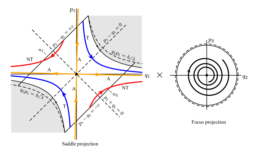
   Figure 5: The flow in the equilibrium region for the dissipative system has the form saddle $\times$ focus. On the left is shown the saddle projection onto the $(q_{1},p_{1})$-plane. The black dot at the origin represents focus-type asymptotic orbits with only a focus projection, thus oscillatory dynamics decaying towards the equilibrium point. The asymptotic orbits (labeled A) are the saddle-type asymptotic orbits which are tilted clockwise compared to the conservative system. They still form the separatrix between transit orbits (T) and non-transit orbits (NT). The hyperbolas, $q_{1}p_{1}=h/\lambda$, are no longer the boundary of trajectories with initial conditions on the bounding sphere ($n_{1}$ or $n_{2}$) due to the dissipation of the energy. The boundary of the shaded region are still the fastest trajectories with initial conditions on the bounding sphere, but are not strictly hyperbolas. Note that the saddle projection and focus projection are uncoupled in this dissipative system.

   Such orbits are asymptotic to the equilibrium point itself, rather than a periodic orbit of energy $h$ as in the conservative case. Due to the effect of damping, the periodic orbits on each energy manifold of energy $h$ do not exist. The 1-sphere $S_{h}^{1}$ still exists, but is no longer invariant. Instead, it corresponds to all the initial conditions of initial energy $h$ which are focus-type asymptotic orbits. The projection of $S_{h}^{1}$ to the configuration space in the dissipative system is the same as the projection of the periodic orbit in the conservative system.

2. The four half open segments on the lines governed by $q_{1}=c_{h}p_{1}/(2\lambda\pm\sqrt{c_{1}^{2}+4\lambda^{2}})$ correspond to saddle-type asymptotic orbits. See the four orbits labeled A in Figure 5.

3. The segments which cross $\mathcal{R}$ from one boundary to the other, i.e., from $p_{1}-q_{1}=+c$ to $p_{1}-q_{1}=-c$ in the northern hemisphere, and vice versa in the southern hemisphere, correspond to transit orbits. See the two orbits labeled $T$ of Figure 5.

4. Finally the segments which run from one hemisphere to the other hemisphere on the same boundary, namely which start from $p_{1}-q_{1}=\pm c$ and return to the same boundary, correspond to non-transit orbits. See the two orbits labeled NT of Figure 5.

As done in Section 2.1, we define the transition region, $\mathcal{T}_{h}$, as the region of initial conditions of a given initial energy $h$ which transit from one side of the neck region to the other. As before, the transition region, $\mathcal{T}_{h}$, is made up of one half which goes to the right, $\mathcal{T}_{h+}$, and the other half which goes to the left, $\mathcal{T}_{h-}$. The boundaries are $\partial\mathcal{T}_{h+}$ and $\partial\mathcal{T}_{h-}$, respectively. The closure of $\partial\mathcal{T}_{h}$, $\overline{\partial\mathcal{T}_{h}}$, is equal to the boundaries $\partial\mathcal{T}_{h+}$ and $\partial\mathcal{T}_{h-}$, along with the focus-type asymptotic initial conditions $S^{1}_{h}$, i.e., as before, $\partial\mathcal{T}_{h-}\cup\partial\mathcal{T}_{h+}\cup S^{1}_{h}$.

As shown below, for the dissipative case, the closure of the boundary of the transition region, $\partial\mathcal{T}_{h}$, has the topology of an ellipsoid, rather than a cylinder as in the conservative case. As before, for convenience, we may refer to $\partial\mathcal{T}_{h}$ and $\overline{\partial\mathcal{T}_{h}}$ interchangeably.

McGehee representation

Similar to the McGehee representation for the conservative system given in Section 2.2 to visualize the region $\mathcal{R}$, here we utilize the McGehee representation again to illustrate the behavior in same region for the dissipative system. All labels are consistent throughout the paper.

Note that since the McGehee representation uses spheres with the same energy to show the dynamical behavior in phase space, while the energy of any particular trajectory in the dissipative system decreases gradually during evolution, Figures 6(b) and 6(c) show only the initial conditions at a given initial energy. Therefore, in the present McGehee representation, only the initial conditions on the two bounding spheres are shown and discussed in the next part. In addition, the black dot near the orange dots $a_{i}^{\pm}$ and $b_{i}^{\pm}$ ($i=1,2$) in Figure 6(b) are the corresponding dots in the conservative system which are used to show how damping affects the transition.

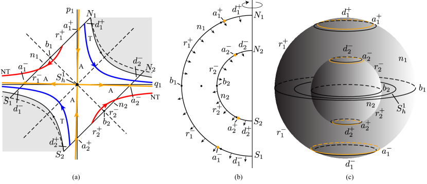
Figure 6: (a) The projection onto the $(q_{1},p_{1})$-plane, the saddle projection, with labels consistent with the text and (b) and (c). (b) The cross-section of the flow in the $\mathcal{R}$ region of the energy surface. The north and south poles of bounding sphere $n_{i}$ are labeled as $N_{i}$ and $S_{i}$, respectively. (c) The McGehee representation of the flow in the region $\mathcal{R}$.

The following classifications of orbits correspond to the previous four categories:

1. 1-sphere $S_{h}^{1}$ exists in the region $\mathcal{R}$ corresponding to the black dot in the middle of Figure 6(b) and the equator of the central 2-sphere given by $p_{1}-q_{1}=0$ in 6(c). The 1-sphere gives the initial conditions of the initial energy $h$ for all focus-type asymptotic orbits. The same 1-sphere in the conservative system is invariant under the flow, that is, a periodic orbit of constant energy $h$. However, the corresponding $S_{h}^{1}$ is not invariant in the dissipative system, since the energy is decreasing during evolution due to the damping.

2. There are four 1-spheres in the region $\mathcal{R}$ starting in the bounding 2-spheres $n_{1}$ and $n_{2}$ which give the initial conditions for orbits asymptotic to the equilibrium point. Two of them in $n^{+}$, labeled by $a^{+}$, are stable saddle-type asymptotic orbits and the other two in $n^{-}$, labeled by $a^{-}$, are unstable asymptotic orbits, where $a^{+}$ and $a^{-}$ are given by,

   $$a_{1}^{+}=\left\{(q_{1},p_{1},q_{2},p_{2})\in\mathcal{R}|\hskip 7.22743pt(q_{1},p_{1})=(k_{p},1)c/(1-k_{p})\right\},$$ (44)

   $$a_{1}^{-}=\left\{(q_{1},p_{1},q_{2},p_{2})\in\mathcal{R}|\hskip 7.22743pt(q_{1},p_{1})=(-1,k_{p})c/(1+k_{p})\right\},$$

   $$a_{2}^{+}=\left\{(q_{1},p_{1},q_{2},p_{2})\in\mathcal{R}|\hskip 7.22743pt(q_{1},p_{1})=(k_{p},1)c/(k_{p}-1)\right\},$$

   $$a_{2}^{-}=\left\{(q_{1},p_{1},q_{2},p_{2})\in\mathcal{R}|\hskip 7.22743pt(q_{1},p_{1})=(1,-k_{p})c/(1+k_{p})\right\},$$

   where $k_{p}=c_{h}/(2\lambda+\sqrt{c_{h}^{2}+4\lambda^{2}})$. As shown in Figure 6(c), $a^{+}$ appears as an orange circle in $n^{+}$, and $a^{-}$ appears as an orange circle in $n^{-}$. The corresponding curves for the same energy in the conservative system are shown as black curves.

3. Consider the two spherical caps on each bounding 2-sphere, $n_{1}$ and $n_{2}$, given by,

   $$d_{1}^{+}=\left\{(q_{1},p_{1},q_{2},p_{2})\in\mathcal{R}\mid\hskip 7.22743ptp_{1}-q_{1}=c,\hskip 7.22743ptq_{1}>ck_{p}/(1-k_{p})\right\},$$ (45)

   $$d_{1}^{-}=\left\{(q_{1},p_{1},q_{2},p_{2})\in\mathcal{R}\mid\hskip 7.22743ptp_{1}-q_{1}=c,\hskip 7.22743ptq_{1}<-c/(1+k_{q})\right\},$$

   $$d_{2}^{+}=\left\{(q_{1},p_{1},q_{2},p_{2})\in\mathcal{R}\mid\hskip 7.22743ptp_{1}-q_{1}=-c,\hskip 7.22743ptq_{1}<ck_{p}/(k_{p}-1)\right\},$$

   $$d_{2}^{-}=\left\{(q_{1},p_{1},q_{2},p_{2})\in\mathcal{R}\mid\hskip 7.22743ptp_{1}-q_{1}=-c,\hskip 7.22743ptq_{1}>c/(1+k_{p})\right\}.$$

   The spherical cap $d_{1}^{+}$, bounded by the $a_{1}^{+}$ on $n_{1}^{+}$, gives all initial conditions of initial energy $h$ for the transit orbits starting from the bounding sphere $n_{1}^{+}$ and entering $\mathcal{R}$. Similarly, the spherical cap $b_{1}^{-}$ in $n_{1}^{-}$, bounded by $a_{1}^{-}$, determines all initial conditions of initial energy $h$ for transit orbits starting on the bounding sphere $n_{1}^{-}$ and leaving $\mathcal{R}$. The spherical caps $d_{2}^{+}$ and $d_{2}^{-}$ on $n_{2}$ have similar dynamical behavior. Note that in the conservative system the transit orbits entering $\mathcal{R}$ on $d^{+}$ will leave on $d^{-}$ in the same 2-sphere. However, those transit orbits with the same initial conditions in the dissipative system will not leave on the corresponding 2-sphere, but leave on another sphere with lower energy. Moreover, the spherical caps $d^{+}$ shrink and $d^{-}$ expand compared to that of the conservative system. Since the area of the caps $d^{+}$ and $b^{-}$ determines the amount of transit orbits and non-transit orbits respectively, the shrinkage of the caps $d^{+}$ and expansion of the caps $d^{-}$ means the damping reduces the probability of transition and increase the probability of non-transition, respectively.

4. Let $b$ be the intersection of $n^{+}$ and $n^{-}$ (where $q_{1}+p_{1}=0$). Then, $b$ is 1-sphere of tangency points. Orbits tangent at this 1-sphere “bounce off”, i.e., do not enter $\mathcal{R}$ locally. The spherical zones $r_{1}$ and $r_{2}$, bounded by $a^{+}_{i}$ and $a^{-}_{i}$, give the initial conditions for non-transit orbits zone. $r^{+}$, bounded by $a^{+}_{i}$ and $b_{i}$, are the initial conditions of initial energy $h$ for non-transit orbits entering $\mathcal{R}$ and $r^{-}_{i}$ are the initial conditions of initial energy $h$ for non-transit orbits leaving $\mathcal{R}$. Note that unlike the shift of the spherical caps in the dissipative system compared to that of the conservative system, the tangent spheres $b_{1}$ and $b_{2}$ do not move when damping is taken into account. Moreover, in the conservative system, non-transit orbits enter $\mathcal{R}$ on $r^{+}$ and then exit on the same energy bounding 2-sphere through $r^{-}$, but the non-transit orbits in the dissipative system exit on a different 2-sphere with different energy determined by the damping and the initial conditions.

Trajectories in the equilibrium region

From the analysis in the eigenspace, we obtain the general solution for the dissipative system in the original coordinates, that is,

$$\begin{split}\bar{q}_{1}(t)&=\frac{\lambda^{2}-c_{y}}{s_{1}}\left(\bar{k}_{1}e^{\beta_{1}t}-\bar{k}_{2}e^{\beta_{2}t}\right),\\ \bar{q}_{2}(t)&=\frac{\omega_{p}^{2}+c_{x}}{s_{2}}e^{-\delta t}\left(k_{5}\cos{\omega_{d}t}+k_{6}\sin{\omega_{d}t}\right),\end{split}$$ (46)

where $\bar{k}_{1}=k_{1}-k_{3}$ and $\bar{k}_{2}=k_{4}-k_{2}$.

Analogous to the situation in the conservative system, we can still classify the orbits into different classes depending on the limiting behavior of $\bar{q}_{1}$ as $t$ tends to plus or minus infinity. Four different categories of orbits can be obtained:

1. Orbits with $\bar{k}_{1}=\bar{k}_{2}=0$ are focus-type asymptotic orbits.

2. Orbits with $\bar{k}_{1}\bar{k}_{2}=0$ are saddle-type asymptotic orbits.

3. Orbits with $\bar{k}_{1}\bar{k}_{2}>0$ are transit orbits.

4. Orbits with $\bar{k}_{1}\bar{k}_{2}<0$ are non-transit orbits.

Wedge of velocity and ellipse of transition

As discussed in Section 3.1.3, the initial conditions of stable asymptotic orbits in the saddle projection of the phase space should be governed by,

$$q_{1}=k_{p}p_{1},$$ (47)

which governs the stable asymptotic orbits which is the boundary of the transit orbits. For the initial conditions in the position space and symplectic eigenspace, denoted by $\left(\bar{q}_{10},\bar{q}_{20},\bar{p}_{10},\bar{p}_{20}\right)$ and $\left(q_{10},q_{20},p_{10},p_{20}\right)$, respectively, they can be connected by the symplectic matrix (31). By using (47) and the change of variables (29), the Hamiltonian function for asymptotic orbits in the symplectic eigenspace can be rewritten by eliminating $q_{10},q_{20},p_{10},p_{20}$ and $\bar{p}_{10}$, as,

$$\frac{\bar{q}_{10}^{2}}{a_{e}^{2}}+\frac{\bar{q}_{20}^{2}}{b_{e}^{2}}+\frac{\bar{p}_{20}^{2}}{c_{e}^{2}}=1,$$ (48)

where,

$$a_{e}=\sqrt{\frac{h\left(k_{p}-1\right)^{2}\left(\lambda^{2}-c_{y}\right)^{2}}{k_{p}s_{1}^{2}\lambda}},\hskip 14.45377ptb_{e}=\sqrt{\frac{2h\left(\omega_{p}^{2}+c_{x}\right)^{2}}{s_{2}^{2}\omega_{p}}},\hskip 14.45377ptc_{e}=\sqrt{\frac{2h\omega_{p}\left(\omega_{p}^{2}+c_{x}\right)^{2}}{s_{2}^{2}}},$$ (49)

which is geometrically an ellipsoid (topologically a 2-sphere). As (48) is the boundary between transit and non-transit orbits starting at an initial energy $h$, we therefore refer to the object described by (48) as the transition ellipsoid of energy $h$. The critical condition for the existence of real solutions for $\bar{p}_{20}$ requires zero discriminant for (48), that is,

$$\frac{\bar{q}_{10}^{2}}{a_{e}^{2}}+\frac{\bar{q}_{20}^{2}}{b_{e}^{2}}=1,\hskip 14.45377pt\bar{p}_{20}=0,$$ (50)

which is an ellipse in the configuration space called the ellipse of transition, and is merely the configuration space projection of the transition ellipsoid (48), first found in [2]. The ellipse of the transition confines the existence of transit orbits of a given initial energy which means the transit orbits can just exist inside the ellipse. For a specific position $\left(\bar{q}_{10},\bar{q}_{20}\right)$ inside the ellipse, $(\bar{q}_{10}/a_{e})^{2}+(\bar{q}_{20}/b_{e})^{2}<1$, the solutions of $\left(\bar{p}_{10},\bar{p}_{20}\right)$ are written as,

$$\bar{p}_{20}=\pm c_{e}\sqrt{1-\frac{\bar{q}_{10}^{2}}{a_{e}^{2}}-\frac{\bar{q}_{20}^{2}}{b_{e}^{2}}},\hskip 7.22743pt\bar{p}_{10}=\frac{k_{p}+1}{k_{p}-1}\lambda\bar{q}_{10}.$$ (51)

Each pair of $(\bar{p}_{10},\bar{p}_{20})$ determines an angle: $\theta=\arctan(\bar{p}_{20}/\bar{p}_{10})$, which together defines the wedge of velocity. The boundary of the wedge gives the two asymptotic orbits at that position.

Figure 7 gives the projection on the position space in the equilibrium region.

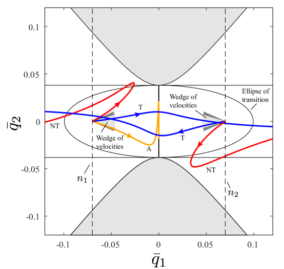
Figure 7: The flow in the equilibrium region $\mathcal{R}$ projected onto position space $(\bar{q}_{1},\bar{q}_{2})$ in the dissipative system with fixed positive energy, $\mathcal{H}_{2}=h>0$, for a ball rolling on a stationary surface. Shown are different types of orbits as discussed in the text. Notice that due to the dissipation of energy, the periodic orbit in the conservative system does not exist, but is replaced by the initial conditions of initial energy $h$ of the focus-type asymptotic orbits. Moreover, the strip for the conservative system—which is the position space projection of the tubes of transition at initial energy $h$—is replaced by the ellipse of transition. It means that the existence of transit orbits are constrained by the ellipse so that the wedge of velocity, determining the permissible direction of the transit orbits, only exist inside the ellipse. For a given fixed energy $h$, the wedge of velocity for the dissipative system is a subset of the wedge for the conservative system which is shown as a darker wedge.

The strip projected onto configuration space in the conservative system which is the boundary of the asymptotic orbits is replaced by the ellipse of transition, which restricts the existence of transition for initial conditions of initial energy $h$ to a locally bounded region. Outside the ellipse, the situation is simple: only non-transit orbits exist. Inside the ellipse, the situation is more complicated since there is a wedge of velocity restricting the direction of transit orbits. The orbits with velocity interior to the wedge are transit orbits, while orbits with velocity outside the wedge are non-transit orbits. The boundary of the wedge gives velocity for the asymptotic orbits. Note that for different point in the position space, the size of the wedge of velocity varies. The closer the wedge is to the boundary of the ellipse of transition, the smaller it is. Clearly, on the ellipse the wedge becomes a line which means only one asymptotic orbit exists there. Note that in the figure, the light grey shaded wedges are the wedges for the dissipative system, while the dark grey shaded wedges partially covered by the light grey ones are for the conservative system of the same initial energy $h$. The significant shrinking of the wedges from the conservative system to the dissipative system is caused by damping. It means an increase in damping decreases the size of the ellipse of transition and wedges on a specific point, which confirms our expectation.

3.1.4 Transition tube and transition ellipsoid

In the position space, we discussed how damping affects the transition. In fact, the strip in the conservative system and ellipse in the dissipative system associated with respective wedges of velocity can predict the transition and non-transition in the corresponding system for a given energy in the position space.

To obtain the initial conditions for asymptotic orbits, the Hamiltonian function for asymptotic orbits has been rewritten in the form of a tube in (38) for the conservative system and the form of an ellipsoid in (48) for the dissipative system, respectively. Here we refer to them as the transition tube and transition ellipsoid, respectively. Compactly, both are $\partial\mathcal{T}_{h}$. See the tube and ellipsoid in Figure 8 and Figure 9, respectively.

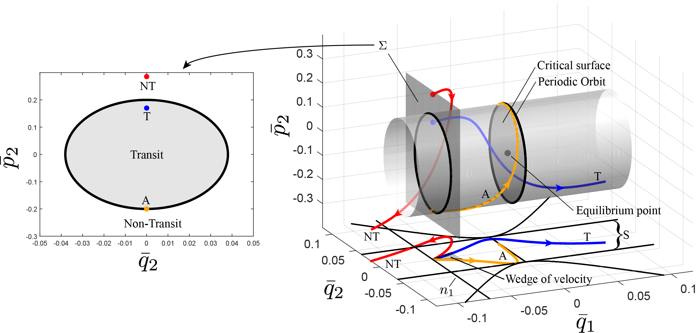
Figure 8: Transition region boundary $\partial\mathcal{T}_{h}$ which is a tube (cylinder) for the conservative system of an idealized ball rolling on a stationary surface with initial energy $h$. The left figure shows tube boundary (the ellipse) separating the transit and non-transit orbits on the Poincaré section $\Sigma$, where the dots are the initial conditions for the corresponding trajectories. The right figure shows the transition tube for a given energy. The critical surface divides the transition tubes into two parts whose left part gives the initial conditions for orbits transitioning to the right, and right part gives the initial conditions for orbits transitioning to the left. Some trajectories are given to show how the transition tube controls the transition whose initial conditions are shown as dots on the left Poincaré section with same color.

In the figures, the tube and the ellipsoid give the boundaries of the initial conditions for transit orbits starting with a given initial energy $h$ in the conservative and the dissipative systems, respectively; all transit orbits must have initial conditions inside the transition tube or transition ellipsoid, respectively; non-transit orbits have initial conditions outside the boundary and asymptotic orbits have initial conditions on the boundary; of course, the periodic orbit not only has initial conditions on the boundary of the transition tube, but also evolves on the boundary. Note that there is a critical surface boundary, given by $S^{1}_{h}$, dividing the tube and ellipsoid into two parts. The left side part is composed of transit orbits going to the right and the right part for transit orbits going to the left.

The orbits with initial conditions on the critical surface $S^{1}_{h}$ are periodic orbits if in the conservative system or focus-type asymptotic orbits if in the dissipative system. The periodic orbit keeps evolving on the critical surface, while the focus-type asymptotic orbit gradually approaches the equilibrium point and finally stops there. The critical surface also plays another important role separating the motion of transit orbits and non-transit orbits. Transit orbits can cross the surface, while non-transit orbits will bounce back before reaching it. Of course, the asymptotic orbits moves asymptotically towards the surface.

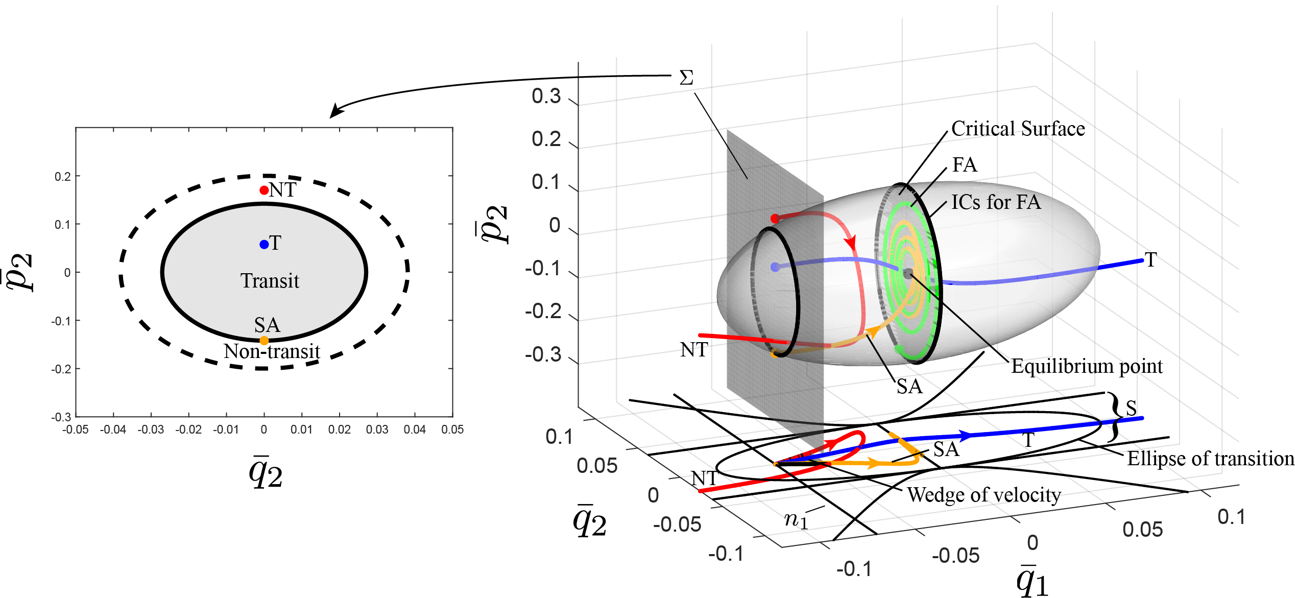
Figure 9: Transition ellipsoid for the dissipative system of a rolling ball on a stationary surface. The left figure shows the Poincaré section $\Sigma$, where the dots are the initial conditions for the corresponding trajectories with the same color in the right figure and the solid ellipse is the set of initial conditions for saddle-type asymptotic orbits. For comparison, the dashed ellipse of the tube boundary for the conservative system with the same energy $h$ is also given. On the right is the ellipsoid giving the initial conditions for all transit orbits. The critical surface divides the ellipsoid into two parts. Each side of the ellipsoid gives the initial conditions of transit orbits passing through the critical surface to the other side. In this figure, SA and FA denote the saddle-type and focus-type asymptotic orbits, respectively.

Illustration of effectiveness

To illustrate the effectiveness of the transition tube and transition ellipsoid, we choose a specific Poincaré section $\Sigma$ revealing the transit region and initial conditions (see dots) of the trajectories shown in the insets of the conservative and dissipative case, respectively. For both the conservative and dissipative systems, the trajectories with initial conditions inside the boundary of the transition can transit from left to right, while trajectories with initial conditions outside of the boundary bounce back to the region where they start; the trajectories with initial conditions on the boundary are asymptotic to a periodic orbit or equilibrium point, for a conservative or dissipative system, respectively. This proves the transition tube and transition ellipsoid can effectively estimate the transition initial conditions in the conservative system and dissipative system, respectively.

It should be noted from the Poincaré section in the dissipative system that the transit region for the dissipative system (see the area encompassed by the solid closed curve) is smaller than the transit region for the conservative system (see the area encompassed by the dashed closed curve) for the same initial energy $h$. The decrease in the area for the transition is caused by the dissipation of the energy. In fact the transit orbit in the conservative system and the non-transit orbit in the dissipative system plotted in the figure have the same initial conditions which means the dissipation of energy can make a transit orbit in the conservative system become a non-transit orbit if dissipation is added.

Up to now, we give the geometry governing the transition in both the position space and phase space. In the position space the strip in the conservative system and the ellipse in the dissipative system are the projections of the outline of the transition tube and transition ellipsoid, respectively. The wedge of velocity on a specific position $(\bar{q}_{1},\bar{q}_{2})$ has two boundaries. The boundaries are the projections of the upper and lower bounds on the corresponding Poincaré section at $\bar{q}_{2}$.

3.2 Snap-through buckling of a shallow arch

Curved structures, like arches/buckled beams [37, 38], shells [39] and domes [40, 41], have many engineering applications. This type of structures can withstand larger transverse loading mainly through membrane stresses compared to flat structures mainly through bending moments. The arch, as an example in this paper, can be at rest in a local minimum of underlying potential energy in unloaded state or under small loading. If subjected to large input of energy or external forces, it may suddenly jump (snap-through) dynamically to another remote local minimum or stable equilibrium. The transition of a buckled conservative nanobeam [42] and macroscopic arch [2] have been studied under the frame of tube dynamics. This section will review the results in [2] where dissipative forces were considered.

Governing equations

In this analysis a slender arch with thickness $d$, width $b$ and length $L$ is considered. A Cartesian coordinate system $xyz$ is established on the mid-plane of the beam in which $x,y$ are the directions along the length and width directions and $z$ the downward direction normal to the mid-plane. Let $u$ and $w$ be the axial and transverse displacements of an arbitrary point on the mid-plane of the beam, respectively, and $w_{0}$ the initial deflection. Based on Euler-Bernoulli beam theory [43, 37], the nonlinear integro-differential governing equation [37, 2, 38] of the beam with in-plane immovable ends is given by,

$$\begin{split}\rho A\frac{\partial^{2}w}{\partial t^{2}}+c_{d}\frac{\partial w}{\partial t}+&EI\left(\frac{\partial^{4}w}{\partial x^{4}}-\frac{\partial^{4}w_{0}}{\partial x^{4}}\right)\\ &+\left[N_{T}-\frac{EA}{2L}\int_{0}^{L}\left(\left(\frac{\partial w}{\partial x}\right)^{2}-\left(\frac{\partial w_{0}}{\partial x}\right)^{2}\right)\mathrm{d}x\right]\frac{\partial^{2}w}{\partial x^{2}}=0,\end{split}$$ (52)

where the boundary conditions of the in-plane immovable ends, $u(0)=u(L)=0$, are applied. See the details of the derivation in [2]. In the equation of motion $\rho$ and $E$ are the mass density and Young’s modulus, respectively; $c_{d}$ is the coefficient of linear viscous damping. $A$ and $I$ are the area and the moment of inertia of the cross-section, respectively, so that $EA$ and $EI$ are the extensional stiffness and bending stiffness. Finally, $N_{T}$ is the axial thermal loading as a convenient way of controlling the initial deflection which replaces the external axial force due to the impossibility of applying such force to the beam with immovable ends. For different types of end constraints, the boundary conditions can be written as,

$$w=0,\quad\frac{\partial^{2}w}{\partial x^{2}}=0,\hskip 36.135pt \text{for simply-simply supported},$$ (53)

$$w=0,\quad\frac{\partial w}{\partial x}=0,\hskip 36.135pt \text{for clamped-clamped supported}.$$

To capture the symmetric and asymmetric snap-through behavior of the arch, the first two mode shapes, $\phi_{1}(x)$ and $\phi_{2}(x)$, will be used. Refs. [2, 15, 37] list the specific forms of $\phi_{i}$ satisfying the boundary conditions of simply-simply supports and clamped-clamped supports which will not be given here for simplification. Assume the deflection and initial imperfection have the following forms,

$$\begin{split}w(x,t)&=X(t)\phi_{1}(x)+Y(t)\phi_{2}(x),\\ w_{0}(x)&=\gamma_{1}\phi_{1}(x)+\gamma_{2}\phi_{2}(x),\end{split}$$ (54)

where $X(t)$ and $Y(t)$ are the amplitudes corresponding to the first two mode shapes of the deflection and $\gamma_{i}$ are the imperfection coefficients. Applying the Galerkin method, one can obtain the following equations of motion for the amplitudes,

$$\begin{split}&M_{1}\ddot{X}+C_{1}\dot{X}+K_{1}\left(X-\gamma_{1}\right)-N_{T}G_{1}X-\frac{EA}{2L}G_{1}^{2}\left(\gamma_{1}^{2}X-X^{3}\right)-\frac{EA}{2L}G_{1}G_{2}\left(\gamma_{2}^{2}X-XY^{2}\right)=0,\\ &M_{2}\ddot{Y}+C_{2}\dot{Y}+K_{2}\left(Y-\gamma_{2}\right)-N_{T}G_{2}Y-\frac{EA}{2L}G_{2}^{2}\left(\gamma_{2}^{2}Y-Y^{3}\right)-\frac{EA}{2L}G_{1}G_{2}\left(\gamma_{1}^{2}Y-X^{2}Y\right)=0,\end{split}$$ (55)

where the coefficients are defined by,

$$\begin{split}\left(M_{i},C_{i}\right)=\left(\rho A,c_{d}\right)\int_{0}^{L}\phi_{i}^{2}\mathrm{d}x,\ \ K_{i}=EI\int_{0}^{L}\left(\frac{\partial^{2}\phi_{i}}{\partial x^{2}}\right)^{2}\mathrm{d}x,\ \ G_{i}=\int_{0}^{L}\left(\frac{\partial\phi_{i}}{\partial x}\right)^{2}\mathrm{d}x.\end{split}$$ (56)

The equations of motion can be re-cast in Hamiltonian form, using the Hamiltonian function $\mathcal{H}=\mathcal{K}+\mathcal{U}$, with $\mathcal{K}$ and $\mathcal{U}$ as in Appendix A.1.

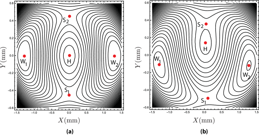
Figure 10: Contours of potential energy, $\mathcal{U}(X,Y)$, of dynamic arch model: (a) the symmetric system, $\gamma_{1}=\gamma_{2}=0$; (b) with small initial imperfections in both modes, i.e., $\gamma_{1}$ and $\gamma_{2}$ are nonzero.

For the parameters selected in [2], we have a fixed two-dimensional potential energy landscape, $\mathcal{U}(X,Y)$, as illustrated in Figure 10. For the arch without initial imperfections, Figure 10(a) shows a symmetric potential energy surface about both $X$ and $Y$. In this system, there are five equilibrium points shown as dots, some of which are stable and some of which are unstable. Of the five points, W₁ and W₂ are the stable equilibrium points, each within its own potential well; S₁ and S₂ are (unstable) saddle points; and H is the unstable hilltop. If the system starts at rest at W₁, it will remain there. If a large impulse with the right size and direction is applied to the arch, it may snap-through, or as understood in phase space, jump to the remote stable equilibrium at W₂, passing close to S₁ or S₂ along the way, and generally avoiding H. If an initial imperfection in both modes is considered, the symmetry of the energy surface about $X$ and $Y$ is broken, as in Figure 10(b). Since we are most interested in the behavior near the saddle points, we linearize the equations about a saddle, either S₁ or S₂, with position $(X_{e},Y_{e})$, which gives the following linearized equations,

$$\begin{split}\dot{x}&=\frac{p_{x}}{M_{1}},\\ \dot{y}&=\frac{p_{y}}{M_{2}},\\ \dot{p}_{x}&=A_{31}x+A_{32}y-C_{H}p_{x},\\ \dot{p}_{y}&=A_{32}x+A_{42}y-C_{H}p_{y},\end{split}$$ (57)

where $(x,y,p_{x},p_{y})=(X,Y,p_{X},p_{Y})-(X_{e},Y_{e},0,0)$ is the displacement from the saddle point in configuration-momentum phase space and the parameters $(A_{31},A_{32},A_{42},C_{H})$ are given in Appendix A.1.

Since Ref. [2] carried out a detailed study on the transition of shallow arch from both a global view, and a local view near the saddle, for both the conservative and dissipative system, the corresponding discussions about the transition are not repeated here . The reader should refer to Ref. [2] for more details. We merely point out that (57) can be non-dimensionalized and transformed into the standard form of (40) in the symplectic eigenspace via a symplectic transformation. The details are given in Appendix A.1.

3.3 Ship motion with equal damping

The stability of ship motion plays an important role in delivery, fishing, transport, and military applications. The phenomenon of capsize has attracted a great amount of attention, due to the ensuing catastrophic losses of life and property. While some studies have only considered single degree-of-freedom dynamics in the roll motion, several studies have concluded that pitch-roll coupling is a much better approximation [44, 45, 46, 47]. However, the consideration of now two coupled degrees of freedom makes the analysis challenging. Under the framework of tube dynamics, Ref. [8] studied nonlinear ship motion and the transition tube for capsize. In addition, the effect of stochastic forcing was taken into account and the skeleton formed by the tube dynamics was shown to persist. However, damping was not taken into consideration in [8]. In this section, we derive the equations of motion with the influence of equal damping along the roll and pitch directions.

Governing equations

Based on [8, 44, 45], we consider the coupled roll and pitch equations for the ship motion of the form,

$$\begin{split}\ddot{\phi}&=-\omega_{\phi}^{2}\phi+2K_{1}\phi\theta+m_{\phi}(t),\\ \ddot{\theta}&=-\omega_{\theta}^{2}\theta+K_{1}\frac{I_{xx}}{I_{yy}}\phi^{2}+m_{\theta}(t),\end{split}$$ (58)

where $\phi$ and $\theta$ are roll and pitch angles measured in radians. The coefficients are defined as,

$$\omega_{\phi}=\sqrt{\frac{K_{\phi}}{I_{xx}}},\hskip 7.22743pt\omega_{\theta}=\sqrt{\frac{K_{\theta}}{I_{yy}}},\hskip 7.22743ptK_{1}=-\frac{K_{\phi\theta}}{2I_{xx}},\hskip 14.45377ptm_{\phi}(t)=\frac{\tau_{\phi}(t)}{I_{xx}},\hskip 7.22743ptm_{\theta}(t)=\frac{\tau_{\theta}(t)}{I_{yy}},$$

where $I_{xx}$ and $I_{yy}$ are the sums of the second moments of inertia and hydrostatic inertia; $K_{\phi}$ and $K_{\theta}$ are the linear rotational stiffness related to the square of the corresponding natural frequency; $K_{\phi\theta}$ is the nonlinear coupling coefficient; $\tau_{\phi}\left(t\right)$ and $\tau_{\theta}\left(t\right)$ are generalized possibly time-dependent torques in the roll and pitch directions, respectively, and $\omega_{\phi}$ and $\omega_{\theta}$ are called the natural roll and natural pitch frequencies, respectively.

For the conservative system, i.e., $m_{\phi}=m_{\theta}=0$, the system has two saddle points at $\left(\pm\phi_{e},\theta_{e}\right)$, with,

$$\phi_{e}=\frac{\omega_{\phi}\omega_{\theta}}{\sqrt{2}K_{1}}\sqrt{\frac{I_{yy}}{I_{xx}}},\hskip 14.45377pt\theta_{e}=\frac{\omega_{\phi}^{2}}{2K_{1}}.$$ (59)

Here $\phi_{e}$ is called the roll angle of vanishing stability and $\theta_{e}$ is the corresponding pitch angle.

The equations of motion (58) can be re-cast in a non-dimensional Hamiltonian form, using a Hamiltonian function $\mathcal{H}$ as given in Appendix A.2. The linearized equations about the saddle points can be written written in matrix form,

$$\dot{\bar{z}}=M\bar{z}+D\bar{z},$$ (60)

where $\bar{z}=\left(\bar{q}_{1},\bar{q}_{2},\bar{p}_{1},\bar{p}_{2}\right)^{T}$ is the displacement from the saddle point in the phase space, and where,

$$M=\begin{pmatrix}0&0&1&0\\ 0&0&0&1\\ 0&1&0&0\\ 1&c_{y}&0&0\end{pmatrix},\hskip 36.135ptD=\begin{pmatrix}0&0&0&0\\ 0&0&0&0\\ 0&0&-c_{h_{1}}&0\\ 0&0&0&-c_{h_{2}}\\ \end{pmatrix}.$$ (61)

The corresponding quadratic Hamiltonian function is given by,

$$\mathcal{H}_{2}=\tfrac{1}{2}\bar{p}_{1}^{2}+\tfrac{1}{2}\bar{p}_{2}^{2}-\bar{q}_{1}\bar{q}_{2}-\tfrac{1}{2}c_{y}\bar{q}_{2}^{2}.$$ (62)

Conservative system

For the conservative system, i.e. $c_{h_{1}}=c_{h_{2}}=0$, one can introduce a change of variables (29) with the symplectic matrix $C$ given by (118) which casts the equations of motion in a simple form in the symplectic eigenspace (3) with Hamiltonian function (1) and solutions (4). The dynamical behavior near the saddle point in both position space and eigenspace are similar to the rolling ball on a stationary surface. Readers can also consult [8] for more details. Note that here further nondimensional parameters were introduced, while Ref. [8] kept them unchanged.

Dissipative system with equal damping

If the coefficients of the viscous damping along both the pitch and roll directions happen to be proportional to the second moments of inertia and hydrostatic inertia, $c_{h_{1}}$ and $c_{h_{2}}$ are exactly the same, denoted by $c_{h}$. Thus, using the same symplectic matrix in (118) one gets the same equations of motion as the standard uncoupled form, (40), in the symplectic eigenspace. For the general case of unequal damping, $c_{h_{1}}\neq c_{h_{2}}$, one will get coupled dynamics on the saddle and focus planes, as shown below in Section 4.2.

4 Coupled systems in the dissipative case

In Section 3, we investigated the geometry of escape/transition in uncoupled systems (in the symplectic eigenspace) which are generally inertial systems with equal damping in each degree of freedom. Due to the uncoupled property, it is easy to obtain the analytical solutions and the dynamical behavior. We have found the transition tube and transition ellipsoid governing the escape in the conservative and dissipative systems, respectively. Another category of system is one in which the saddle and focus are coupled with each other when the system is transformed to the corresponding eigenspace. The situation is more complicated but important and interesting. The first kind is an inertial system with unequal damping, like the ship motion discussed in Section 4.2. Another one is a system with both gyroscopic and dissipative forces present. Such systems can display non-intuitive phenomena, like dissipation-induced instabilities [22] as discussed in the introduction. In this section, we establish the mathematical models for some physical problems and reveal the geometry of escape/transition in such systems.

4.1 Ball rolling on a rotating surface

In Section 3.1, the rolling ball on a stationary surface was studied and the effect of dissipative forces was considered. We established it as a standard example to investigate the escape from a potential well in inertial systems with equal damping and revealing the escape mechanism in such systems. Here we further expand the framework regarding escape to a more complicated situation where the surface is rotating such that gyroscopic forces exist. Several researchers have investigated a ball or particle moving on a rotating surface [22, 23, 24, 48, 49], mainly due to the unexpected dissipation-induced instabilities. The combination of the dissipative and gyroscopic forces enriches the behavior in escape dynamics.

4.1.1 Governing equations

Consider a rotating surface with counterclockwise angular velocity $\omega$ as shown in Figure 11.

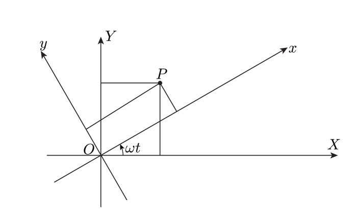
Figure 11: Inetial and rotating frames. The rotating coordinate system of $x$ and $y$ axes moves counterclockwise with constant angular velocity $\omega$ relative to the inertial frame with $X$ and $Y$ axes. The $z$ axis coincides with the $Z$ axis which is pointing out of the plane and is not shown here. We denote the unit vectors along $x$, $y$, $z$ by $\mathbf{e}_{1}$, $\mathbf{e}_{2}$ and $\mathbf{e}_{3}$, respectively.

Let $X\mbox{-}Y\mbox{-}Z$ be an inertial frame, denoted as the $N$ frame, with origin $O$, where $X\mbox{-}Y$ plane is horizontal and $Z$ is vertical to the plane. Establish another rotating frame $x\mbox{-}y\mbox{-}z$, denoted as the $R$ frame, with the same origin $O$ fixed on the rotating surface, where $Oz$ coincides with $OZ$. In this study, the geometrical parameters of the rotating surface are the same as before given in (12).

The angular velocity vector of the $R$ frame relative to the $N$ frame is,

$$\text{\boldmath$\omega$}^{R/N}=\omega\mathbf{e}_{3}.$$ (63)

A particle (or ball), denoted by $P$, with unit mass, moves on the rotating surface, with a position vector described in the $R$ frame as,

$$\mathbf{P}(x,y,z,t)=x(t)\mathbf{e}_{1}+y(t)\mathbf{e}_{2}+z(t)\mathbf{e}_{3},$$ (64)

where $(x,y,z)$ is the position of the mass in the $R$ frame. The inertial velocity of the mass can be written in the $R$ frame as,

$$\begin{split}{}^{N}\mathbf{v}^{P}&=\dot{x}\mathbf{e}_{1}+\dot{y}\mathbf{e}_{2}+\dot{z}\mathbf{e}_{3}+\text{\boldmath$\omega$}^{R/N}\times\mathbf{P}\\ &=\left(\dot{x}-y\omega\right)\mathbf{e}_{1}+\left(y+x\omega\right)\mathbf{e}_{2}+\dot{z}\mathbf{e}_{3}.\end{split}$$ (65)

Considering the motion is constrained on the rotating surface, here $z$ is not an independent variable, but depends on $x$ and $y$ via $z=H(x,y)$. Thus, the kinetic energy $\mathcal{K}$ and potential energy $\mathcal{U}$ are,

$$\begin{split}\mathcal{K}(x,y)&=\tfrac{1}{2}I|^{N}\mathbf{v}^{P}|^{2}=\tfrac{1}{2}I\left[\left(\dot{x}-y\omega\right)^{2}+\left(\dot{y}+x\omega\right)^{2}+\left(H_{,x}\dot{x}+H_{,y}\dot{y}\right)^{2}\right],\\ \mathcal{U}(x,y)&=gH(x,y).\end{split}$$ (66)

After obtaining the Lagrangian function, $\mathcal{L}=\mathcal{K}-\mathcal{U}$, we can derive the Euler-Lagrange equations given in (15). As discussed in [23], two types of damping can be considered in the rotating surface system, i.e., internal damping and external damping. Internal damping is proportional to the relative velocity measured in the rotating frame, while external damping is proportional to the inertial velocity. Thus, the mathematical form of two types of the generalized damping forces are,

$$\begin{split}Q_{x}^{\rm int}&=-c_{d}\left[\left(1+H_{,x}^{2}\right)\dot{x}+H_{,x}H_{,y}\dot{y}\right],\\ Q_{y}^{\rm int}&=-c_{d}\left[\left(1+H_{,y}^{2}\right)\dot{y}+H_{,x}H_{,y}\dot{x}\right],\end{split}\hskip 7.22743pt\text{ for internal damping}$$ (67)

and,

$$\begin{split}Q_{x}^{\rm ext}&=-c_{d}\left[\left(1+H_{,x}^{2}\right)\dot{x}+H_{,x}H_{,y}\dot{y}-\omega y\right],\\ Q_{y}^{\rm ext}&=-c_{d}\left[\left(1+H_{,y}^{2}\right)\dot{y}+H_{,x}H_{,y}\dot{x}+\omega x\right],\end{split}\hskip 7.22743pt\text{ for external damping}$$ (68)

where $c_{d}$ is the coefficient of damping. In the current problem, we only consider internal damping, $(Q_{x},Q_{y})=(Q_{x}^{\rm int},Q_{y}^{\rm int})$, due to the friction between the mass and the moving surface, as the most physically relevant.

The equations of motion can be written in non-dimensional Hamiltonian form, using a Hamiltonian function $\mathcal{H}$ as given in Appendix A.3. Following the same procedure as for the ball rolling on a stationary surface, we linearize the equations of motion around the saddle point at the origin which gives the linearized non-dimensional Hamilton’s equation in matrix form,

$$\dot{\bar{z}}=M\bar{z}+D\bar{z},$$ (69)

where $\bar{z}=\left(\bar{q}_{1},\bar{q}_{2},\bar{p}_{1},\bar{p}_{2}\right)^{T}$ is the displacement from the saddle point, and where,

$$M=\begin{pmatrix}0&\omega&1&0\\ -\omega&0&0&1\\ c_{x}&0&0&\omega\\ 0&c_{y}&-\omega&0\end{pmatrix},\hskip 7.22743ptD=c_{h}\begin{pmatrix}0&0&0&0\\ 0&0&0&0\\ 0&-\omega&-1&0\\ \omega&0&0&-1\end{pmatrix}.$$ (70)

The quadratic Hamiltonian function corresponding to matrix $M$ is,

$$\mathcal{H}_{2}(\bar{q}_{1},\bar{q}_{2},\bar{p}_{1},\bar{p}_{2})=\tfrac{1}{2}\left(\bar{p}_{1}^{2}+\bar{p}_{2}^{2}\right)+\omega\bar{p}_{1}\bar{q}_{2}-\omega\bar{p}_{2}\bar{q}_{1}-\tfrac{1}{2}\left(c_{x}\bar{q}_{1}^{2}+c_{y}\bar{q}_{2}^{2}\right).$$ (71)

4.1.2 Analysis in the conservative system

In this section, the dynamic behavior in the conservative system will be analyzed. Here the damping $c_{h}$ is set to zero which gives,

$$\dot{\bar{z}}=M\bar{z}.$$ (72)

Curiously, we are able to use the eigenvectors of $M$ in (70) and use them to construct a symplectic linear change of variables which changes (72) into the simple normal form (3), with the simple Hamiltonian function (1) and with solutions as given in (4). The details are in Appendix A.3.

Trajectories in the equilibrium region

The flow in the equilibrium region $\mathcal{R}$ in the symplectic eigenspace was performed for the normal form in Section 2 and will not be repeated here. However, it is instructive to study the appearance of the orbits in the position space for this particular problem, i.e., the $\left(\bar{q}_{1},\bar{q}_{2}\right)$ plane. Note that the evolution of all trajectories must be restricted by the given energy $h$ which forms the zero velocity curves [6] (corresponding to $\dot{v}_{x}=\dot{v}_{y}=0$) which bound the motion in the position space projection and are determined by the following function,

$$\bar{q}_{2}\left(\bar{q}_{1}\right)=\pm\sqrt{\frac{-2h-\left(c_{x}+\omega^{2}\right)\bar{q}_{1}^{2}}{c_{y}+\omega^{2}}},$$ (73)

which is obtained from (71).

From the solutions in the symplectic eigenspace (4), we can obtain the general (real) solutions in the position space by using the transformation matrix $C$ in (140) which yields the general (real) solutions with the form (34). Thus, we can obtain the solutions for $\bar{q}_{1}$ and $\bar{q}_{2}$, given the initial conditions in the eigenspace, $(q_{1}^{0},q_{2}^{0},p_{1}^{0},p_{2}^{0})$,

$$\begin{split}\bar{q}_{1}(t)&=\frac{\lambda^{2}-c_{y}-\omega^{2}}{s_{1}}q_{1}^{0}e^{\lambda t}-\frac{\lambda^{2}-c_{y}-\omega^{2}}{s_{1}}p_{1}^{0}e^{-\lambda t}-\frac{2\omega\omega_{p}}{s_{2}}\left(p_{2}^{0}\cos\omega_{p}t-q_{2}^{0}\sin\omega_{p}t\right),\\ \bar{q}_{2}(t)&=-\frac{2\lambda\omega}{s_{1}}q_{1}^{0}e^{\lambda t}-\frac{2\lambda\omega}{s_{1}}p_{1}^{0}e^{-\lambda t}-\frac{\omega_{p}^{2}+c_{x}+\omega^{2}}{s_{2}}\left(q_{2}^{0}\cos\omega_{p}t+p_{2}^{0}\sin\omega_{p}t\right).\\ \end{split}$$ (74)

Upon inspecting the general solution, we see that the solutions on the energy surface fall into different classes depending upon the limiting behavior of $\bar{q}_{1}(t)$ as $t$ tends to plus or minus infinity. As the $\bar{q}_{1}(t)$ expression is dominated by the $q_{1}^{0}$ term as $t\rightarrow+\infty$, $\bar{q}_{1}$ tends to minus infinity (staying on the left-hand side), is bounded (staying around the equilibrium point), or tends to plus infinity (staying on the right-hand side) for $q_{1}^{0}>0$, $q_{1}^{0}=0$ and $q_{1}^{0}<0$, respectively. The statement holds if $t\rightarrow-\infty$ and $-p_{1}^{0}$ replaces $q_{1}^{0}$. Varying the signs of $q_{1}^{0}$ and $p_{1}^{0}$, and following the procedures described in [2, 31], one can also obtain the same nine classes of orbits grouped into the same four categories as in Section 3.1.

1. If $q_{1}^{0}=p_{1}^{0}=0$, we obtain a periodic solution with the following projection onto the position space,

   $$\frac{\bar{q}_{1}^{2}}{\left(\frac{2\omega\omega_{p}}{s_{2}}\sqrt{\frac{2h}{\omega_{p}}}\right)^{2}}+\frac{\bar{q}_{2}^{2}}{\left(\frac{\omega_{p}^{2}+c_{x}+\omega^{2}}{s_{2}}\sqrt{\frac{2h}{\omega_{p}}}\right)^{2}}=1.$$ (75)

   Here, the initial energy is $h=\frac{1}{2}\omega_{p}\left[(q_{2}^{0})^{2}+(p_{2}^{0})^{2}\right]$. Identical to what has been proved by Conley [31] for the restricted three-body problem, this periodic orbit, shown in Figure 12, projects onto the $\left(\bar{q}_{1},\bar{q}_{2}\right)$ plane as an ellipse. Note that the size of the ellipse goes to zero with $h$. It is different from the non-gyroscopic system where the periodic orbit projects to a straight segment in the position space.

2. Orbits with $q_{1}^{0}p_{1}^{0}=0$ are asymptotic orbits. They are asymptotic to the periodic orbits of category 1. The asymptotic orbit with $q_{1}^{0}=0$ projects into the strip $S_{1}$ in the $\left(\bar{q}_{1},\bar{q}_{2}\right)$ plane bounded by the lines,

   $$\bar{q}_{2}=\frac{2\lambda\omega}{\lambda^{2}-c_{y}-\omega^{2}}\bar{q}_{1}\pm\sqrt{\left(\frac{4\lambda\omega_{p}\omega^{2}}{s_{2}\left(\lambda^{2}-c_{y}-\omega^{2}\right)}\right)^{2}+\left(\frac{\omega_{p}^{2}+c_{x}+\omega^{2}}{s_{2}}\right)^{2}}\sqrt{\frac{2h}{\omega_{p}}},$$ (76)

   while orbits with $p_{1}^{0}=0$ project into the strip $S_{2}$ bounded by the lines,

   $$\bar{q}_{2}=-\frac{2\lambda\omega}{\lambda^{2}-c_{y}-\omega^{2}}\bar{q}_{1}\pm\sqrt{\left(\frac{4\lambda\omega_{p}\omega^{2}}{s_{2}\left(\lambda^{2}-c_{y}-\omega^{2}\right)}\right)^{2}+\left(\frac{\omega_{p}^{2}+c_{x}+\omega^{2}}{s_{2}}\right)^{2}}\sqrt{\frac{2h}{\omega_{p}}}.$$ (77)

   In fact, $S_{1}$ is for stable asymptotic orbits, while $S_{2}$ is for unstable asymptotic orbits. Notice the width of the strips depend on $h$ and go to zero as $h\rightarrow 0$.

3. Orbits with $q_{1}^{0}p_{1}^{0}>0$ are transit orbits because they cross the equilibrium region $\mathcal{R}$ from $-\infty$ (the left-hand side) to $+\infty$ (the right-hand side) or vice versa.

4. Orbits with $q_{1}^{0}p_{1}^{0}<0$ are non-transit orbits.

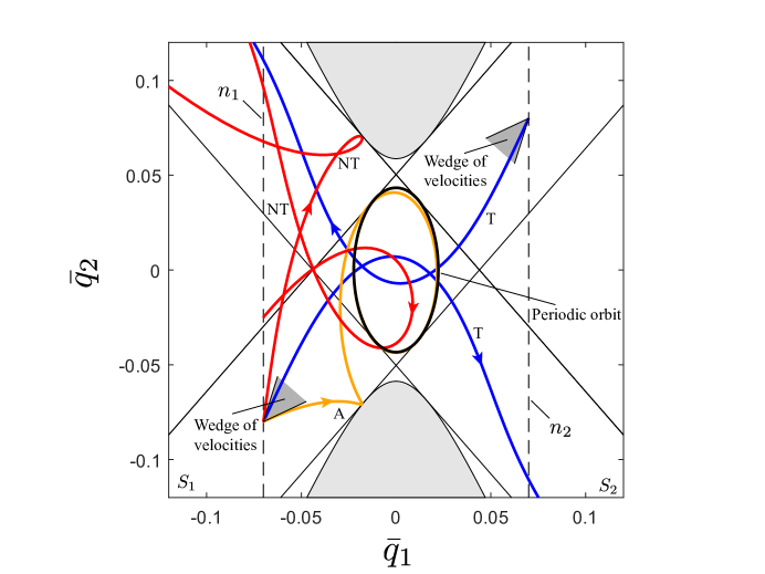
Figure 12: The flow in the equilibrium region $\mathcal{R}$ projected onto position space $(\bar{q}_{1},\bar{q}_{2})$ in the conservative system with fixed positive energy, $\mathcal{H}_{2}=h>0$, for a ball rolling on a rotating surface. Shown are the periodic orbit acting as an ellipse; one asymptotic orbit gradually approaching the periodic orbit; two transit orbits; and two non-transit orbits, one starting inside the strips and the other outside the strips. Note that the dynamic behavior in the position space is identical to those in the circular restricted three-body problem [4, 5].

The wedge of velocity

To study the projection of the last two categories of orbits in the restricted three-body problem, Conley [31] proved a couple of propositions to determine whether at each position, $\left(\bar{q}_{1},\bar{q}_{2}\right)$, the wedge of velocity exists, in which $q_{1}^{0}p_{1}^{0}>0$. See the shaded wedges in Figure 12. In the current problem, the same behavior is observed. In the next part, the derivation will be given by a more direct method than Conley’s, developed in [2] for the more general dissipative system. Note that the orbits with velocity on the boundary of a wedge satisfy $q_{1}^{0}p_{1}^{0}=0$, making them asymptotic orbits (which will be used in the derivation).

For initial conditions $\left(\bar{q}_{1}^{0},\bar{q}_{2}^{0},\bar{p}_{1}^{0},\bar{p}_{2}^{0}\right)$ in the original phase space and $\left(q_{1}^{0},q_{2}^{0},p_{1}^{0},p_{2}^{0}\right)$ in the symplectic eigenspace, we can establish their relations by the symplectic matrix $C$ in (140), i.e., $\left(\bar{q}_{1}^{0},\bar{q}_{2}^{0},\bar{p}_{1}^{0},\bar{p}_{2}^{0}\right)^{T}=C\left(q_{1}^{0},q_{2}^{0},p_{1}^{0},p_{2}^{0}\right)^{T}$. Note that we have $q_{1}^{0}=0$ and $p_{1}^{0}=0$ for stable and unstable asymptotic orbits, respectively. We can then express $p_{1}^{0}$ (or $q_{1}^{0}$), $q_{2}^{0}$, $p_{2}^{0}$ and $\bar{p}_{2}^{0}$ in terms of $\bar{q}_{1}^{0}$, $\bar{q}_{2}^{0}$ and $\bar{p}_{1}^{0}$. After substituting $q_{2}^{0}$ and $p_{2}^{0}$ as a function of $\bar{q}_{1}^{0}$, $\bar{q}_{2}^{0}$ and $\bar{p}_{1}^{0}$ into the Hamiltonian normal form (1) we can rewrite (1) for asymptotic orbits as,

$$a_{p}\left(\bar{p}_{1}^{0}\right)^{2}+b_{p}\bar{p}_{1}^{0}+c_{p}=0,$$ (78)

where $a_{p}$, $b_{p}$, and $c_{p}$ are found in Appendix A.3 and depend on $i=1,2$ for stable ($q_{1}^{0}=0$) and unstable ($p_{1}^{0}=0$) asymptotic orbits, respectively. Thus, we can obtain the strips $S_{i}$ $(i=1,2)$ by taking the determinant, $\bar{\Delta}=b_{p}^{2}-4a_{p}c_{p}$, of the quadratic equation (78) to be zero (i.e., $\bar{\Delta}=0$) which are exactly the same expressions as that in (76) and (77).

For $\bar{\Delta}>0$, we obtain two real values for $\bar{p}_{1}^{0}$ as,

$$\bar{p}_{1}^{0}=\frac{-b_{p}\pm\sqrt{b_{p}^{2}-4a_{p}c_{p}}}{2a_{p}},$$ (79)

and then the expression for $\bar{p}_{2}^{0}$ is obtained as,

$$\bar{p}_{2}^{0}=\frac{\bar{p}_{1}^{0}\lambda\left(1+c_{x}+\omega_{p}^{2}\right)}{2\left(1+c_{x}\right)}+\frac{\left(1+c_{x}-\omega_{p}^{2}\right)\left[\bar{q}_{2}^{0}\lambda+\left(1+c_{x}\right)\bar{q}_{1}^{0}\right]}{2\left(1+c_{x}\right)}.$$ (80)

Therefore, the two initial velocities formed by the two asymptotic orbits can result in the wedge of velocity with wedge angle $\theta=\arctan\left(\bar{p}_{2}^{0}/\bar{p}_{1}^{0}\right)$.

Up to now, we have obtained the strips and wedge of velocity. In Figure 12, $S_{1}$ and $S_{2}$ are the two strips mentioned above. Outside of each strip $S_{i}\left(i=1,2\right)$, the sign of $q_{1}^{0}$ and $p_{1}^{0}$ is independent of the direction of the velocity. These signs can be determined in each of the components of the equilibrium region $\mathcal{R}$ complementary to both strips. For example, in the left-most central components, $q_{1}^{0}$ is negative and $p_{1}^{0}$ is positive, while in the right-most central components $q_{1}^{0}$ is positive and $p_{1}^{0}$ is negative. Therefore, $q_{1}^{0}p_{1}^{0}<0$ in both components and only non-transit orbits project onto these two components.

Inside the strips the situation is more complicated since the sign of $q_{1}^{0}p_{1}^{0}$ depends on the direction of the velocity. For simplicity we have indicated this dependence only on the two vertical bounding line segments in Figure 12. For example, consider the intersection of strip $S_{1}$ with the left most vertical line. On this subsegment, there is at each point a wedge of velocity in which $q_{1}^{0}$ is positive. The sign of $p_{1}^{0}$ is always positive on this segment, so orbits with velocity interior to the wedge of velocity are transit orbits $\left(q_{1}^{0}p_{1}^{0}>0\right)$. Of course, orbits with velocity on the boundary of the wedge are asymptotic $\left(q_{1}^{0}p_{1}^{0}=0\right)$, while orbits with velocity outside of the wedge are non-transit $\left(q_{1}^{0}p_{1}^{0}<0\right)$. In Figure 12, only one transit and one asymptotic orbit starting on this subsegment are illustrated. The situation on the remaining three subsegments is similar.

4.1.3 Analysis in the dissipative system

Recall that in the dissipative system of the rolling ball on a stationary surface the saddle projection and focus projection in the eigenspace of the conservative system (i.e., the symplectic eigenspace) are uncoupled. The transition is only determined by the location in the saddle projection and energy. However, when the surface is rotating, the situation is different. To compare the behavior in the different systems, we utilize the same change of variables as in (140), i.e., $\bar{z}=Cz$, and the equations of motion in the symplectic eigenspace are,

$$\dot{z}=\Lambda z+\Delta z,$$ (81)

where $\Lambda=C^{-1}MC$ from before, (33), but the transformed damping matrix is now,

$$\Delta=C^{-1}DC=c_{h}K,$$ (82)

where $K$ is a $4\times 4$ matrix with many non-zero components, given in (142) in Appendix A.3.

Notice that for the rolling ball on a stationary surface discussed in Section 3.1.3 and the dynamical buckling of a shallow arch [2] in the dissipative system, the canonical planes $\left(q_{1},p_{1}\right)$ and $\left(q_{2},p_{2}\right)$ have their dynamics uncoupled. Here, however, the dynamics on the $\left(q_{1},p_{1}\right)$ and $\left(q_{2},p_{2}\right)$ planes are coupled due to the combination of dissipative and gyroscopic forces. We see this coupling via several coupling terms which are no longer zero in (142), e.g., $K_{12}$, $K_{14}$, $K_{21}$ and $K_{23}$, etc. Because of the coupling between the $\left(q_{1},p_{1}\right)$ and $\left(q_{2},p_{2}\right)$ planes, it is difficult to obtain simple analytical solutions in the symplectic eigenspace variables. Thus, the semi-analytical method which substitutes all the parameters into the equations will be used to analyze the linear behavior near the saddle point.

One can obtain a fourth-order characteristic polynomial for the matrix $\Lambda+\Delta$ from which to obtain eigenvalues. Here we denote the four eigenvalues as $\beta_{1},-\beta_{2},\beta_{3,4}=-\delta\pm iw_{d}$, where $\beta_{1},\beta_{2},\delta$ and $\omega_{d}$ are all positive real numbers. Note that the saddle $\times$ center type equilibrium point in the conservative system becomes a saddle $\times$ focus type equilibrium point in the dissipative system. The four corresponding generalized eigenvectors are denoted as $u_{1}$, $u_{2}$ and $u_{3}\pm iu_{4}$, where $u_{i}$ are all real vectors. Thus, the general solutions to system (81) can be expressed as,

$$z(t)=k_{1}^{0}u_{1}e^{\beta_{1}t}+k_{2}^{0}u_{2}e^{-\beta_{2}t}+e^{-\delta t}\mathrm{Re}\left[k_{0}e^{-i\omega_{d}t}\left(u_{3}-iu_{4}\right)\right],$$ (83)

where $k_{1}^{0}$ and $k_{2}^{0}$ are real and $k_{0}=k_{3}^{0}+ik_{4}^{0}$ is complex ($k_{3}^{0}$ and $k_{4}^{0}$ are real).

The flow in the equilibrium region

Analogous to the discussion for the conservative system, we still choose the same equilibrium region $\mathcal{R}$ determined by $\mathcal{H}_{2}=h$ and $|p_{1}-q_{1}|\leq c$ with positive $h$ and $c$. Due to the coupling between the saddle projection and focus projection, the behavior in the eigenspace is complicated. When $t\rightarrow+\infty$ and $t\rightarrow-\infty$, $z$ is dominated by the $k_{1}^{0}$ term and $k_{2}^{0}$ term, respectively. Thus, one can categorize the orbits into different groups based solely on the signs of $k_{1}^{0}$ and $k_{2}^{0}$. However, the visualization of all the initial conditions for different types of orbits specified by a given energy is indirect. To do so, setting the initial conditions in the symplectic eigenspace as $z_{0}=(q_{1}^{0},q_{2}^{0},p_{1}^{0},p_{2}^{0})$, the following relation between the symplectic and dissipative eigenspace variables is obtained,

$$\begin{split}\begin{pmatrix}q_{1}^{0}\\ q_{2}^{0}\\ p_{1}^{0}\\ p_{2}^{0}\end{pmatrix}=\begin{pmatrix}\vdots&\vdots&\vdots&\vdots\\ u_{1}&u_{2}&u_{3}&u_{4}\\ \vdots&\vdots&\vdots&\vdots\end{pmatrix}\begin{pmatrix}k_{1}^{0}\\ k_{2}^{0}\\ k_{3}^{0}\\ k_{4}^{0}\end{pmatrix},\end{split}$$ (84)

where the eigenvectors $u_{i}$ are written as column vectors.

As discussed for the conservative system, asymptotic orbits play an important role, acting as the separatrix of transit orbits and non-transit orbits. Moreover, the size of stable asymptotic orbits determines the amount of transit orbits. A straightforward method to obtain the stable asymptotic orbits, analogous to what was done for the conservative case, is as follows. For the stable asymptotic orbits, we have $k_{1}^{0}=0$. Then we can use (84) to obtain $k_{i}^{0}$ $(i=2,3,4)$ and $p_{2}^{0}$ in terms of $q_{1}^{0}$, $q_{2}^{0}$ and $p_{1}^{0}$. Analogous to the situation for the conservative system in Section 2.1, we select the initial conditions on two sets $n_{1}$ and $n_{2}$ projecting to the line segments $p_{1}^{0}=q_{1}^{0}\pm c$. Substituting $p_{2}^{0}$ in terms of $q_{1}^{0}$, $q_{2}^{0}$ and $p_{1}^{0}$ and the relation $q_{1}^{0}=p_{1}^{0}\mp c$ into the Hamiltonian normal form (1), we rewrite it in exactly the same form as in (78): $a_{p}\left(p_{1}^{0}\right)^{2}+b_{p}p_{1}^{0}+c_{p}=0$. Note that here $a_{p}$, $b_{p}$ and $c_{p}$ are functions of $q_{20}$ which are different to that in (78). To guarantee $p_{1}^{0}$ has real solutions, $\bar{\Delta}=b_{p}^{2}-4a_{p}c_{p}>0$ should be true. Thus, we can obtain $q_{20}^{(l)}<q_{2}^{0}<q_{20}^{(u)}$, where $q_{20}^{(l)}$ and $q_{20}^{(u)}$ are the lower and upper bounds for $q_{2}^{0}$. For different $q_{2}^{0}\in\left[q_{20}^{(l)},q_{20}^{(u)}\right]$, we can obtain $p_{1}^{0}=\left(-b_{p}\pm\sqrt{b_{p}^{2}-4a_{p}c_{p}}\right)/(2a_{p})$ and thus obtain $q_{1}^{0}$ and $p_{2}^{0}$.

Null space method

Another method to obtain the stable asymptotic orbits, here called the null space method, can also be utilized. The procedure is as follows: (1) using three generalized eigenvectors corresponding to the eigenvalues with negative real part (i.e., $u_{2}$, $u_{3}$, $u_{4}$), the null space of the stable eigenspace, $E^{s}=\mathrm{span}\{u_{2},u_{3},u_{4}\}$, can be obtained, denoted as $u_{n}=\left(u_{n1},u_{n2},u_{n3},u_{n4}\right)^{T}$, with the relation $u_{n}\cdot u_{i}=0$ $(i=2,3,4)$; (2) Since the initial conditions $z_{0}$ of forward asymptotic orbits (i.e., stable asymptotic orbits) should be normal to the null space, we have $u_{n}\cdot z_{0}=0$, which, along with the Hamiltonian function, will give the same quadratic equation, $a_{p}\left(p_{1}^{0}\right)^{2}+b_{p}p_{1}^{0}+c_{p}=0$; (3) following the same manipulation as described in the previous paragraph, we obtain the same results.

Flow in the equilibrium region

Different combinations of the signs of $k_{1}^{0}$ and $k_{2}^{0}$ gives nine classes of orbits which can be grouped into the same four categories as the dissipative system of the rolling ball on a stationary surface. All initial conditions on the bounding lines $n_{1}$ and $n_{2}$ for different types of orbits can be visualized based on the analysis listed below.

1. Orbits with $k_{1}^{0}=k_{2}^{0}=0$ corresponds to a focus-type asymptotic orbit with motion in the $\left(q_{2},p_{2}\right)$ plane (see black dot at the origin of the $\left(q_{1},p_{1}\right)$ plane in Figure 13). Due to the effect of energy dissipation, the periodic orbit does not exist.

2. Orbits with $k_{1}^{0}k_{2}^{0}=0$ are saddle-type asymptotic orbits. For example, the bolded orange line on the bounding line $n_{1}$ in the saddle projection associated with the closed solid curve in the focus projection in Figure 13 are all the initial conditions for the stable asymptotic orbits with initial conditions of initial energy $h$ on $n_{1}$. Because of the coupling between the saddle projection and focus projection, one point on the closed solid curve in the focus projection has a corresponding point on the bolded region in saddle projection which together give the initial condition for a specific asymptotic orbit of initial energy $h$. See the orange dots for the initial condition of the stable asymptotic orbit starting from $n_{1}$ and orange curve for the evolution. Of course, the bounding line $n_{2}$ has the behavior for the stable asymptotic orbits. Since the system just has one positive eigenvalue, the unstable asymptotic orbits just have one specific direction along each side of the saddle point. See the orange straight lines for the unstable asymptotic orbits. Four asymptotic orbits are shown in Figure 13 labeled A.

3. The segments determined by $k_{1}^{0}k_{2}^{0}<0$ which cross $\mathcal{R}$ from the bounding line $n_{1}$ to the bounding line $n_{2}$ in the northern hemisphere, and vice versa in the southern hemisphere, correspond to the transit orbits with initial energy $h$ on $n_{1}$ and $n_{2}$, respectively. See the two example orbits labeled T of Figure 13.

4. Finally the segments with $k_{1}^{0}k_{2}^{0}>0$ which start from one hemisphere and bounce back are the non-transit orbits of initial energy $h$. See the two orbits labeled NT in Figure 13.

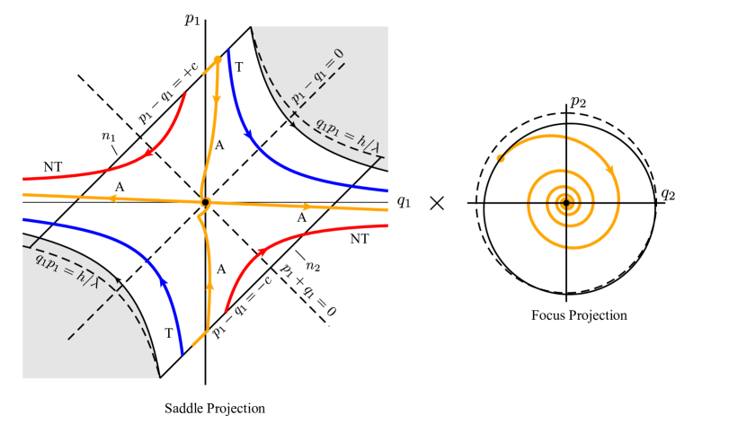
Figure 13: The flow in the equilibrium region $\mathcal{R}$ projected onto $(q_{1},p_{1})$ plane and $(q_{2},p_{2})$ plane which are coupled has form saddle $\times$ focus. Shown are the saddle-type asymptotic orbits (labeled A), transit orbits (labeled T) and non-transit orbits (labeled NT). The dot at the origin of $(q_{1},p_{1})$ plane is the focus-type asymptotic orbits with projection only on $(q_{2},p_{2})$ plane which is a damped oscillator decaying to the origin. Due to the coupling between $(q_{1},p_{2})$ plane and $(q_{2},p_{2})$ plane, the initial conditions for the three-dimensional stable asymptotic orbit are dependent on the angle in focus projection. The one dimensional unstable asymptotic orbits are a straight line in the saddle projection.

McGehee representation

The previous section gives the topological structure of initial conditions for different types of orbits in the dissipative system, but it still may not be intuitive. Thus, as we did in the rolling ball on a stationary surface, we introduce the McGehee representation to visualize the region $\mathcal{R}$ for easier interpretation. Since there are many curves on the two 2-spheres, $n_{1}$ and $n_{2}$, of initial energy $h$, we show the two spheres separately in Figure 14(c).

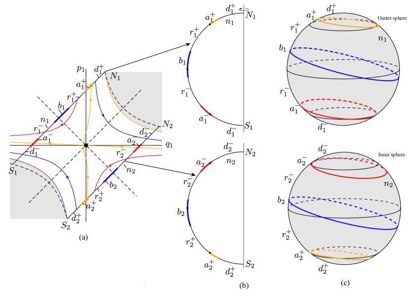
Figure 14: The McGehee representation of the equilibrium region for dissipative system of rolling ball on a rotating surface. (a) The projection of flow onto $(q_{1},p_{1})$ plane. (b) The projection of the flow in the $\mathcal{R}$ region of the energy surface onto a cross-section. (c) The McGehee representation of the flow on the boundaries of the $\mathcal{R}$ region, highlighting the features on the bounding spheres $n_{1}$ and $n_{2}$, the “inner” and “outer” spheres, respectively.

As mentioned in the ball rolling on a stationary surface with damping, the McGehee representation gives the spheres with the same energy $h$ so that here the McGehee representation again just shows the initial conditions on each bounding sphere. The symbols in Section 2.2 have the same meaning as used here. The previous four categories of orbits are interpreted as follows.

1. There is a 1-sphere $S_{h}^{1}$ in the region $\mathcal{R}$, similar to that in the rolling ball on a stationary surface with dissipation, which is the equator of the 2-sphere given by $p_{1}-q_{1}=0$. The set $S_{h}^{1}$ gives the initial conditions for the focus-type asymptotic orbits with initial energy $h$. Readers are referred to the dot in Figure 6(b) for interpretation.

2. There are two 1-spheres represented by the orange closed curves on each bounding sphere, denoted by $a^{+}_{i}$ and $a^{-}_{i}$ on sphere $n_{i}$. They give the initial conditions for stable asymptotic orbits. Compared to the ball rolling on a stationary surface, which has initial conditions for stable asymptotic orbits given by circles on the bounding spheres parallel to the corresponding equators, initial conditions for stable asymptotic orbits for the rotating surface are tilted. This is due to dissipation-induced coupling of the saddle and focus projections of the symplectic eigenspace. Note that the unstable asymptotic orbits are one-dimensional and have different energy from the bounding sphere so that they cannot be given in the McGehee representation.

3. Consider the two spherical caps on each bounding 2-sphere denoted by $d_{1}^{+}$, $d_{1}^{-}$ and $d_{2}^{+}$, $d_{2}^{-}$. The transit orbits with initial conditions on spherical cap $d_{1}^{+}$, which is in $n_{1}^{+}$ and bounded by $a_{1}^{+}$, enter $\mathcal{R}$ and leave through $n_{2}$ at a different (lower) energy, due to dissipation. On the other hand, the transit orbits with initial conditions on spherical cap $d_{1}^{-}$ in $n_{1}^{-}$ bounded by $a_{1}^{-}$ are leaving $\mathcal{R}$ having entered through $n_{2}$ at a different (higher) energy. An analogous situation holds on bounding sphere $n_{2}$.

4. There is a 1-sphere of tangency points, denoted by $b$, with initial conditions on which the orbits do not enter $\mathcal{R}$ locally. To obtain the tangency points, first we need to the recognize the relation along each angle $\theta$ in the focus projection, i.e. $p_{2}^{0}=q_{2}^{0}\tan\theta$, as well as the initial conditions on the bounding spheres $n_{1}$ and $n_{2}$, i.e. $p_{1}^{0}=q_{1}^{0}\pm c$, and the tangency conditions, i.e. $\dot{p}_{1}^{0}=\pm\dot{q}_{1}^{0}$. We then substitute such relations into the Hamiltonian normal form to yield a quadratic equation which will give two tangency points along that angle. Note that the 1-spheres here are not the equators of the bounding spheres, as they are in the non-rotating case, but are tilted by an angle compared with the conservative system, again, due to the coupling via the dissipation matrix $K$, from (142). The topological hemisphere above $b_{1}$ in $n_{1}$ is referred to as $n_{1}^{+}$ and below $b_{1}$ as $n_{1}^{-}$; similarly for $n_{2}$, as illustrated in Figure 14(c). Similar to before, the non-transit orbits with initial conditions of initial energy $h$ on spherical zone $r^{+}_{i}$, in $n^{+}_{i}$ bounded by $a^{+}_{i}$ and $b_{i}$, are entering $\mathcal{R}$ and non-transit orbits with initial conditions on spherical zone $r^{-}_{i}$, in $n^{-}_{i}$ bounded by $a^{+}_{i}$ and $b_{i}$, are leaving $\mathcal{R}$.

Trajectories in the equilibrium region

Following the standard procedure to solve (69), we get the eigenvalues of the matrix $M+D$ (denoted as as $\bar{\beta}_{1},-\bar{\beta}_{2},\bar{\beta}_{3,4}=-\bar{\delta}\pm i\bar{w}_{d}$, where $\bar{\beta}_{1},\bar{\beta}_{2},\bar{\delta}$ and $\bar{\omega}_{d}$ are positive real values) associated with the corresponding generalized eigenvectors (denoted as $\bar{u}_{i}\hskip 7.22743pt(i=1,2,3,4)$). The general real solutions to (69) are,

$$\bar{z}(t)=\bar{k}_{1}^{0}\bar{u}_{1}e^{\bar{\beta}_{1}t}+\bar{k}_{2}^{0}\bar{u}_{2}e^{-\bar{\beta}_{2}t}+e^{-\bar{\delta}t}\mathrm{Re}\left[\bar{k}_{0}e^{-i\bar{\omega}_{d}t}\left(\bar{u}_{3}-i\bar{u}_{4}\right)\right],$$ (85)

where $\bar{k}_{1}^{0}$ and $\bar{k}_{2}^{0}$ are real and $\bar{k}_{0}=\bar{k}_{3}^{0}+i\bar{k}_{4}^{0}$ is complex. By inspecting the limiting behavior of $\bar{q}_{1}$ as $t$ tends to plus or minus infinity, we can also obtain the following four categories of orbits:

1. Orbits with $\bar{k}_{1}^{0}=\bar{k}_{2}^{0}=0$ are focus-type asymptotic orbits. When dissipation is considered in the system, the periodic orbit does not exist, but these initial conditions correspond to purely focus-like dynamics, with an amplitude decreasing proportional to $e^{-\bar{\delta}t}$.

2. Orbits with $\bar{k}_{1}^{0}=0$ ( or $\bar{k}_{2}^{0}=0$) are stable (or unstable) saddle-type asymptotic to the saddle equilibrium point.

3. Orbits with $\bar{k}_{1}^{0}\bar{k}_{2}^{0}>0$ are transit orbits.

4. Orbits with $\bar{k}_{1}^{0}\bar{k}_{2}^{0}<0$ are non-transit orbits.

Wedge of velocity and ellipse of transition

As discussed previously, for this rotating system one also obtains an ellipse of transition which confines the existence of transit orbits. Inside the ellipse, the transit orbits exist, while outside the ellipse transit orbits do not exist. As before, a non-empty wedge of velocity, which divides the transit orbits from the non-transit orbits, can only exist inside the ellipse of transition.

Taking $t=0$, one obtains the relation between the initial conditions $\bar{z}_{0}=\left(\bar{q}_{1}^{0},\bar{q}_{2}^{0},\bar{p}_{1}^{0},\bar{p}_{2}^{0}\right)$ and the coefficients $\bar{k}_{i}^{0}$ with a similar form as in (84). For stable asymptotic orbits, i.e., $\bar{k}_{1}^{0}=0$, we can determine the coefficients $\bar{k}_{i}^{0}(i=2,3,4)$ and $\bar{p}_{20}$ in terms of initial conditions $\bar{q}_{10},\bar{q}_{20},\bar{p}_{10}$. With the substitution of $\bar{q}_{1}^{0},\bar{q}_{2}^{0},\bar{p}_{1}^{0}$ and $\bar{p}_{2}^{0}$ into (71), the quadratic Hamiltonian (71) restricted by energy $h$ can be rewritten as a second order algebraic equation for $\bar{p}_{1}^{0}$ which has exactly the same form as (78), but with different $a_{p},b_{p}$ and $c_{p}$ in terms of $\bar{q}_{1}^{0}$ and $\bar{q}_{2}^{0}$. On the one hand, for the critical condition, i.e., $\vartriangle=b_{p}^{2}-4a_{p}c_{p}=0$, we can obtain an ellipse of transition which is different from the strips $S_{1}$ in the conservative system. The ellipse limits the location of transit orbit initial conditions. On the other hand, when the determinant satisfies $\vartriangle=b_{p}^{2}-4a_{p}c_{p}>0$, $\bar{p}_{1}^{0}$ has two real solutions, $\bar{p}_{1}^{0}=\left(-b_{p}\pm\sqrt{b_{p}^{2}-4a_{p}c_{p}}\right)/\left(2a_{p}\right)$, associated with two real solutions for $\bar{p}_{2}^{0}$. Thus, the two pairs of results of $\left(\bar{p}_{1}^{0},\bar{p}_{2}^{0}\right)$ will determine two bounding directions of velocity, which form the wedge of velocity.

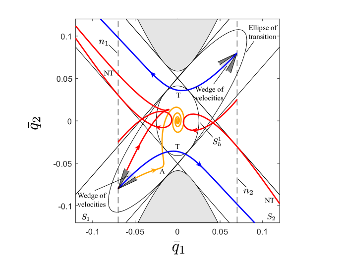
Figure 15: The flow in the equilibrium region $\mathcal{R}$ of position space. Shown are the saddle-type asymptotic orbit; two transit orbits; three non-transit orbits. For the same given energy, the wedges of velocity for the dissipative system (the smaller light grey shaded wedges), restricted by the ellipse of transition, partially cover the wedges of velocity for the conservative system (the larger dark grey shaded wedges) restricted by a strip.

Figure 15 shows the flow in the projection of the equilibrium region $\mathcal{R}$ to position space, taking gyroscopic and dissipative effects into consideration. Due to energy dissipation, the strips which are the boundaries of asymptotic orbits in the position space of the conservative system no longer exist. In particular, the strip for the stable asymptotic orbit is replaced by the ellipse of transition. The ellipse of transition, similar to the role in the rolling ball on a stationary surface, confines the existence of transit orbits. That is, transit orbits of a given initial energy $h$ must have initial conditions inside the ellipse of transition, while only non-transit orbit initial conditions project onto the area complementary of the ellipse. However, even if the initial condition of an orbit projects to a position inside the ellipse of transition, this alone does not guarantee the transition. This is a necessary but not a sufficient condition. The additional condition is that the velocity should be along certain directions. The wedge of velocity obtained above, which is non-empty only inside the ellipse, is exactly the condition providing the correct range of directions for the velocity of transit orbits. Orbits with initial conditions interior to the wedge can transit, while orbits with velocity outside the wedge cannot transit. The orbits with velocity on the boundary of the wedge are asymptotic to the equilibrium point.

The sizes of the wedge of velocity and ellipse of transition, which both represent the proportion of transit orbits compared to non-transit orbits, are dependent on the energy, $h$, and the amount of damping, $c_{h}$. An increase of energy gives more transit orbits, while an increase in damping reduces the proportion of transit orbits. Furthermore, different positions inside the ellipse have different sizes of wedges of velocity. The closer the position is to the boundary of the ellipse of transition, the smaller the size of the wedge of velocity will be. From Figure 15, we find that the size of the wedge shrinks (light grey) compared with that of the conservative system (dark grey) which qualitatively indicates how damping affects the wedge of velocity.

4.1.4 Transition tube and transition ellipsoid

We have discussed the flow in the position space for a rolling ball on a rotating surface near a saddle point. In this section, we will visualize the structures governing transitions in the phase space, particularly on surfaces of constant initial energy $h$.

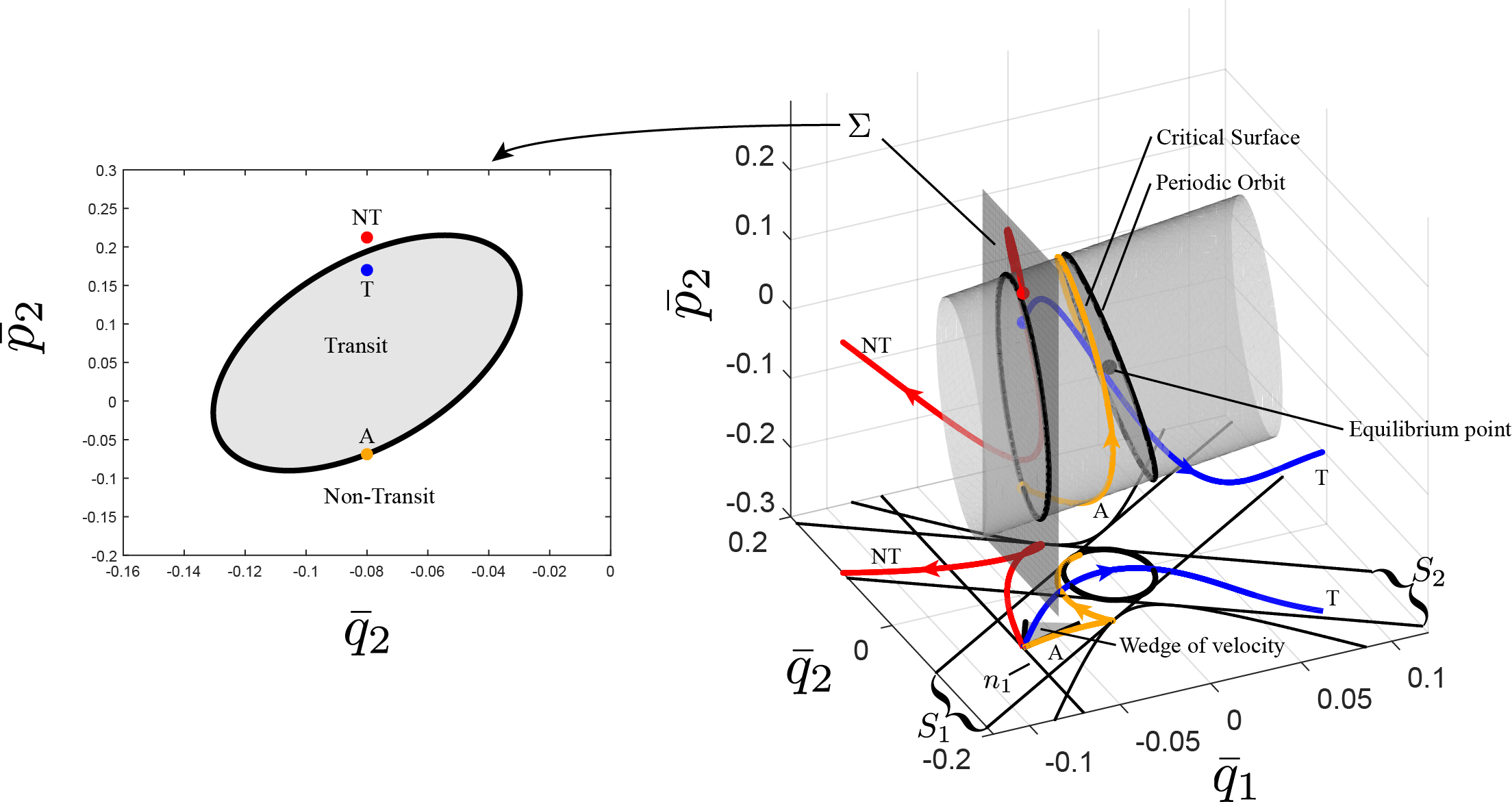
Figure 16: Transition tube for the ball rolling on a rotating surface. The left figure gives the region for initial conditions of transit orbits on the Poincaré section $\Sigma$ with three initial conditions (the dots) for three types of orbits. The right shows the transition tube for a given energy. The critical surface playing the same role as the ball rolling on a stationary surface also exists here. Three types of orbits with initial conditions on the left figure are given.

For the rolling ball on a stationary surface, we obtained the transition tube and transition ellipsoid that give all the initial conditions, starting at a given initial energy $h$, of transit orbits for the conservative system and dissipative system, respectively. In the current problem, we have similar phase space structures governing the transition which can be obtained by the semi-analytical method mentioned before. Figure 16 and Figure 17 show the transition tube and transition ellipsoid, respectively. As discussed in Section 3.1.4, for a specific energy all transit orbits in the conservative system and dissipative system must have initial conditions inside the transition tube and transition ellipsoid, respectively; all orbits with initial conditions outside the transition tube and transition ellipsoid are non-transit orbits. Furthermore, the critical surface divides the transition tube and transition ellipsoid into two parts. Orbits with initial conditions inside the left part will transit to the right and orbits with initial conditions inside the right part will transit to the left. Orbits on the boundary are asymptotic to the periodic orbit (respectively, equilibrium point) in the conservative (respectively, dissipative) system. Transit orbits can cross the critical surface, while non-transit orbits will bounce back before reaching the critical surface.

Figure 16 and Figure 17 also give different types of orbits with the initial conditions on the same Poincaré section in the corresponding system. This illustrates the discussion given above that transit orbits must have initial conditions inside the transition tube or transition ellipsoid. In fact, the transit orbit (initial condition marked T in Figure 16) in the conservative system and the non-transit orbit (initial condition marked NT in Figure 17) in the dissipative system have the same initial condition. This demonstrates that initial conditions corresponding to a transit orbit in the conservative system may be non-transit orbits if damping is taken into account.

It is worth noting that the topological structures in phase space controlling the transition for both the non-rotating system and rotating system are almost the same. Nevertheless, differences exist between these two systems. In the non-rotating system, the axes of the transition tube and transition ellipsoid are parallel to the position space axes, while in the rotating system, the axes of the transition tube and transition ellipsoid is not parallel to the position space axes, but are tilted by an angle.

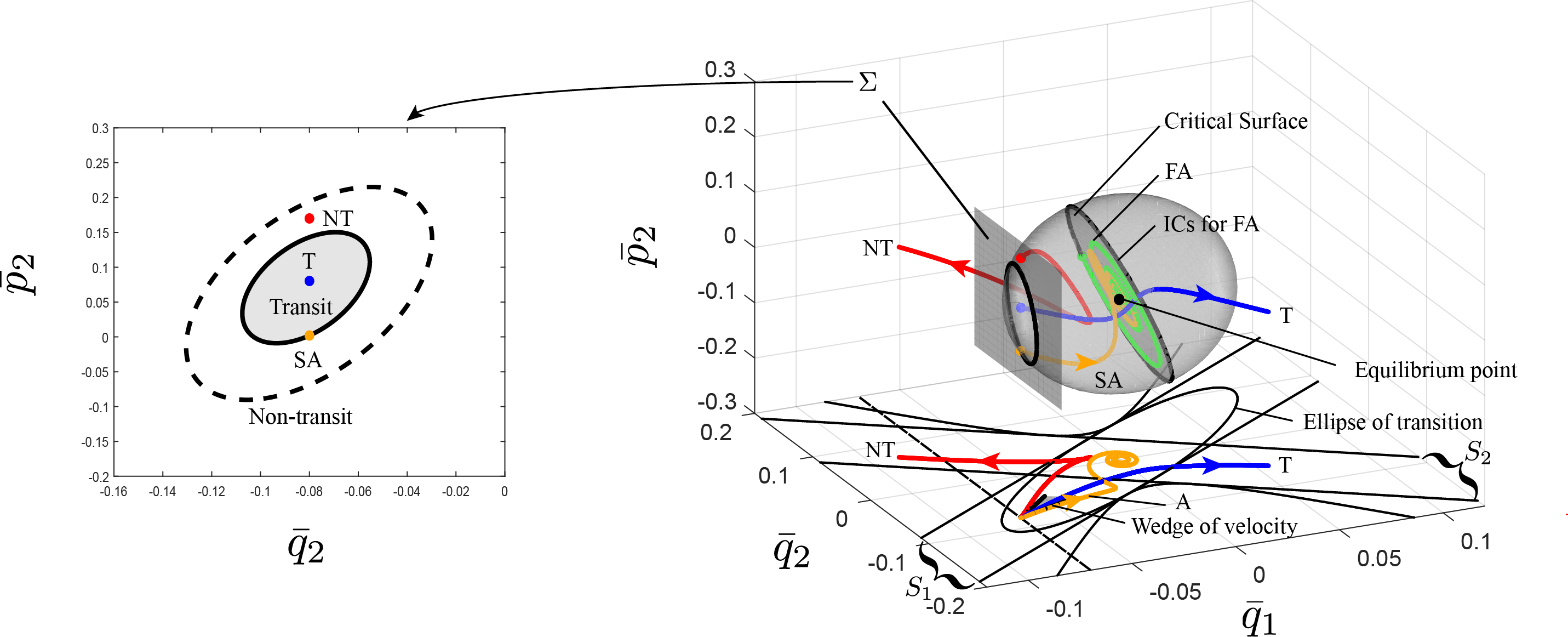
Figure 17: Transition ellipsoid for the dissipative system in the rolling ball on a rotating surface. The left figure shows the Poincaré section $\Sigma$, where the dots are the initial conditions for the corresponding trajectories and the solid ellipse is the boundary of initial conditions for the transit orbits. For comparison, the dashed ellipse of tube boundary for the conservative system is also given. For The right figure shows the transition tube with three different types of orbits with initial conditions on the left figure.

4.2 Ship motion with unequal damping

In Section 3.3, we derived the equations of motion of a ship considering the coupled roll-pitch motion with damping. When the coefficients of damping happen to be equal, the equations of motion projected into the symplectic eigenspace have uncoupled saddle projection and focus projection dynamics. However, the situation becomes more complicated if unequal damping is considered, since the saddle and focus projections in the symplectic eigenspace become coupled. This case is similar to the rolling ball on a rotating surface with dissipation. Since the analysis has been given in Section 4.1, here we simply give the equations of motion with unequal damping transformed into the symplectic eigenspace.

The equations of motion linearized about the saddle point, (60), under the same symplectic transformation as described in Section 3.3, becomes,

$$\dot{z}=\Lambda z+\Delta z,$$ (86)

where $\Lambda=C^{-1}MC$ is the standard matrix of the conservative part of the dynamics (33), but the transformed damping matrix is,

$$\Delta=\Delta_{1}+\delta c_{h}\tilde{\Delta},$$ (87)

where $\Delta_{1}$ is the standard uncoupled damping matrix (41), with $c_{h}=c_{h_{1}}$, $\delta c_{h}=c_{h_{2}}-c_{h_{1}}$ is the difference between the two damping coefficients, and $\tilde{\Delta}$ is given in (124). The matrix $\tilde{\Delta}$ contains terms which couple the dynamics on the two canonical planes, $(q_{1},p_{1})$ and $(q_{2},p_{2})$, and this coupling vanishes only when $\delta c_{h}=0$, i.e., when the two damping coefficients are equal. See Appendix A.2 for details.

4.3 The restricted three-body problem with dissipation

The restricted three-body problem is a classic problem which has attracted a lot of attention for the study of escape [4, 5, 6, 50, 51, 52, 53, 54, 55, 56, 57, 58, 59, 60, 61, 62, 63]. Deeper understanding of the escape from a gravitational potential well due to multiple bodies can guide the design of trajectories for interplanetary space missions and also aid analysis of certain astronomical phenomena (e.g., galactic dynamics [64, 65, 66, 67, 68, 69, 70]). When dissipation is taken into account, the situation becomes more complicated, but becomes applicable to a larger number of situations, such as drag due to interplanetary dust [27, 71], and engineering applications, such as low thrust [72] and solar sails [73, 74].

We formulate the planar circular restricted three-body problem (PCR3BP) using a standard approach [28, 27, 6]. Without loss of generality, the total mass of the two main bodies are normalized to unity, denoted by $m_{1}=1-\mu$ and $m_{2}=\mu$, respectively, where $\mu$ is the non-dimensional mass parameter. Masses $m_{1}$ and $m_{2}$ orbit in a plane counterclockwise in circles about their common center of mass with angular velocity also normalized to one. A third body (spacecraft or small object) denoted by $P$, whose mass is ignored as too small to influence $m_{1}$ or $m_{2}$ significantly, can move freely in the $m_{1}$-$m_{2}$ orbital plane under the effect of their combined gravitational field. Denote the position of $P$ by $(x,y)$ in a co-orbiting or rotating frame whose $x$-axis coincides with the line connecting the two main bodies, with the origin at the center of mass, as shown in Figure 18.

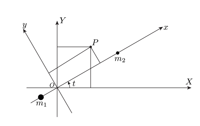
Figure 18: Inertial and rotating frames in restricted three-body problem. The rotating coordinate system of $x$ and $y$ axes moves counterclockwise with unit angular velocity relative to the inertial frame with $X$ and $Y$ axes.

From the Lagrangian point of view, the non-dimensional equations of motion of $P$ are,

$$\ddot{x}-2\dot{y}=-\mathcal{U}_{,x}+Q_{x},\hskip 14.45377pt\ddot{y}+2\dot{x}=-\mathcal{U}_{,y}+Q_{y},$$ (88)

where the (effective) potential energy, which includes both gravitational and centrifugal forces, is,

$$\mathcal{U}(x,y)=-\tfrac{1}{2}(x^{2}+y^{2})-\frac{1-\mu}{r_{1}}-\frac{\mu}{r_{2}}-\tfrac{1}{2}\mu(1-\mu),$$

where $r_{1}=\sqrt{(x+\mu)^{2}+y^{2}}$ and $r_{2}=\sqrt{(x-1+\mu)^{2}+y^{2}}$ are the distances of $P$ from $m_{1}$ and $m_{2}$, respectively. The generalized forces $Q_{x}$ and $Q_{y}$ are the components of damping along $x$ and $y$, respectively. After applying the Legendre transformation to the Lagrangian formulation, the Hamiltonian function is,

$$\mathcal{H}=\tfrac{1}{2}\left[\left(p_{x}+y\right)^{2}+\left(p_{y}-x\right)^{2}\right]+\mathcal{U}(x,y),$$ (89)

which yields the following Hamilton’s equations,

$$\dot{x} =p_{x}+y,$$ (90)

$$\dot{y} =p_{y}-x,$$

$$\dot{p}_{x} =p_{y}-x-\mathcal{U}_{,x}+Q_{x},$$

$$\dot{p}_{y} =-p_{x}-y-\mathcal{U}_{,y}+Q_{y}.$$

Conservative system

For the conservative system, we have $Q_{x}=Q_{y}=0$. In this case, the system has five equilibrium points, three collinear equilibria on the $x$-axis, labeled $L_{1}$, $L_{2}$, $L_{3}$ and two equilateral points labeled $L_{4}$ and $L_{5}$. These equilibrium points are critical points of the (effective potential) function $\mathcal{U}$. In this study, we focus on the behavior of particle trajectories near the two Lagrange points, $L_{1}$ and $L_{2}$, on either side of the (smaller) secondary mass, $m_{2}$. Here $L$ is used to denote either point $L_{1}$ or $L_{2}$. To find the linearized equations around the collinear libration point $L$ with coordinates $(x_{e},y_{e},p_{xe},p_{ye})=(x_{e},0,0,x_{e})$, we do the following. After making a coordinate change with $(x_{e},0,0,x_{e})$ as the origin, the quadratic terms form a Hamiltonian function for the linearized equations, given by [6],

$$\mathcal{H}_{2}=\tfrac{1}{2}(p_{x}^{2}+p_{y}^{2})+yp_{x}-xp_{y}-\bar{\mu}x^{2}+\tfrac{1}{2}\bar{\mu}y^{2},$$ (91)

where the only parameter, $\bar{\mu}>1$, is defined by,

$$\bar{\mu}=\mu|x_{e}-1+\mu|^{-3}+(1-\mu)|x_{e}+\mu|^{-3}.$$ (92)

A short computation gives the linearized equations in the canonical Hamiltonian form,

$$\dot{x} =p_{x}+y,$$ (93)

$$\dot{y} =p_{y}-x,$$

$$\dot{p}_{x} =2\bar{\mu}x+p_{y},$$

$$\dot{p}_{y} =-\bar{\mu}y-p_{x}.$$

Following the same procedure as other problems, one can find the change of variables via a symplectic matrix $C$ given by (143), which transforms the quadratic Hamiltonian (91) into the simple form (3). See Appendix A.4 and [6] for details. The dynamic behavior near the equilibrium in both the symplectic eigenspace and configuration space are the same as that of the rolling ball on a rotating surface from Section 4.1.

Dissipative system

In this part, we consider the linearization around the point $L$ with damping included. As is mentioned in Section 4.1, there are two types of damping in a rotating system, internal damping and external damping. Internal damping, proportional to the relative velocity in the rotating frame, is also called simple nebular drag [75] in celestial mechanics. To obtain the equilibrium point, one seeks the set corresponding to $\dot{x}=\dot{y}=0$. Thus, one can conclude the equilibrium point $L$ does not shift compared with the conservative system. Since its dynamical behavior is similar to those discussed in the rolling ball on a rotating system with internal damping, readers can refer to Section 4.1 for details.

On the other hand, external damping, proportional to the velocity with respect to the inertial frame, is also called the inertial drag force [75]. In this case, generally the equilibrium points will shift. Ref. [75] gives some approximate formulas to determine the location of the equilibrium point $L$ for systems with sufficiently small drag forces. In general, for small drag, the equilibrium point $L$ keeps $x_{e}$ approximately constant, but $y_{e}$ moves away from zero, becoming increasingly negative with increasing $c_{h}$. For a large drag force, numerical tools have to be used to find the equilibrium points. See Figure 19, the right panel, for a curve, a 1-parameter family, of how the equilibria corresponding to $L_{1}$ and $L_{2}$ shift for increasing $c_{h}$.

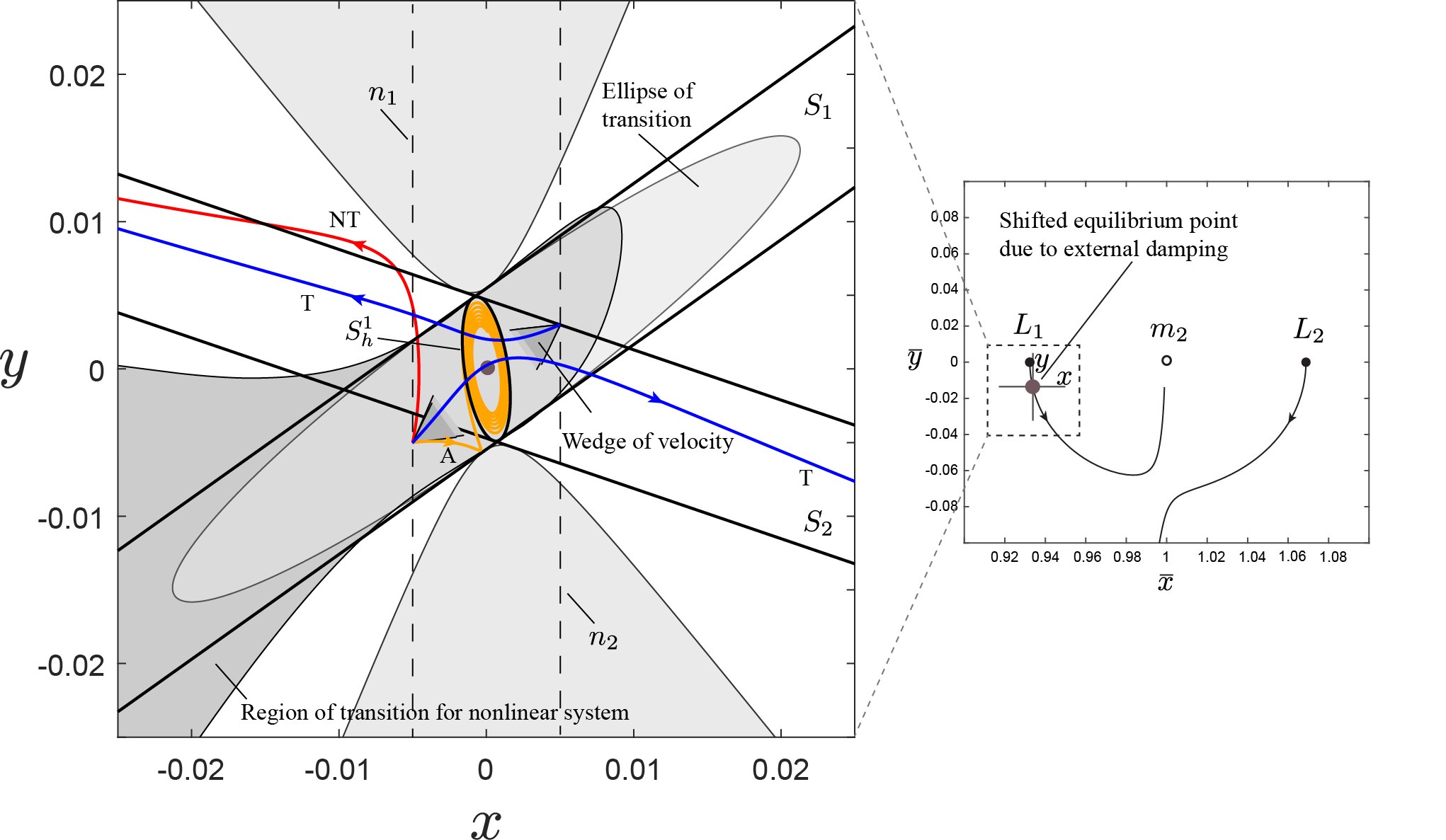
Figure 19: In the right panel, we show the original rotating axes with bars, $(\bar{x},\bar{y})$, for the PCR3BP with external damping, where here the $\bar{x}$-axis is along the $m_{1}$-$m_{2}$ line. We also show the curve of equilibrium point positions $L_{1}$ and $L_{2}$ as a function of the damping coefficient $c_{h}$, starting at $c_{h}=0$ for the black dots on the $\bar{x}$-axis, with $c_{h}$ increasing away from these points. In the left panel, we show the flow in the equilibrium region $\mathcal{R}$ projected onto position space $(x,y)$, which are the displacement from the now-shifted $L_{1}$ equilibrium point (gray dot in both panels). Shown are a saddle-type asymptotic orbit (labeled A); two transit orbits (labeled T) and a non-transit orbit (labeled NT). The larger light grey shaded ellipse and the dark grey shaded region are boundaries of initial conditions of all possible transit orbits for linearized system and nonlinear system with equal quadratic terms whose common area is the medium gray shaded region. The smaller ellipse close to the origin is periodic orbit and the two strips, labeled $S_{1}$ and $S_{2}$, are the boundary of asymptotic orbits in effective conservative system which does not exist physically. In this figure, the Sun-Jupiter system is used with mass parameter $\mu=9.537\times 10^{-4}$; the damping coefficient is taken as $c_{h}=0.05$.

We note that there are other types of drag forces, like solar radiation pressure, Poynting-Robertson drag, solar wind drag [76, 77], and Stokes drag [78]. For internal and external linear damping in the non-dimensionalized PCR3BP problem, the formulas are generally,

$$\begin{split}Q_{x}^{\rm int}&=-c_{h}\dot{x},\\ Q_{y}^{\rm int}&=-c_{h}\dot{y},\end{split}\hskip 7.22743pt\text{ for internal damping}$$ (94)

and,

$$\begin{split}Q_{x}^{\rm ext}&=-c_{h}(\dot{x}-y),\\ Q_{y}^{\rm ext}&=-c_{h}(\dot{y}+x),\end{split}\hskip 7.22743pt\text{ for external damping}$$ (95)

where $c_{h}$ is the non-dimensional coefficient of damping.

For simplicity, only external damping will be considered in the numerical computations that follow, as it leads to new phenomena. We focus on the equilibrium point $L_{1}$. We denote the shifted equilibrium point by $(x_{e},y_{e},-y_{e},x_{e})$ , where $y_{e}$ is now non-zero, and shifted from $L_{1}$ in the conservative system. Linearizing the Hamilton’s equations in (90) about the equilibrium point results in the following linearized equations in Hamiltonian form,

$$\dot{x} =p_{x}+y,$$ (96)

$$\dot{y} =p_{y}-x,$$

$$\dot{p}_{x} =b_{1}x+b_{2}y+p_{y}-c_{h}p_{x},$$

$$\dot{p}_{y} =b_{2}x+b_{3}y-p_{x}-c_{h}p_{y},$$

where $(x,y)$ are now the small displacement from the shifted equilibrium $(x_{e},y_{e})$ with $(p_{x},p_{y})$ the conjugate momenta. The matrix representation of (96) is in the form $M+D$, where $M$ is the conservative part coming from a Hamiltonian function, and $D$ comes from damping. This system can be written as resulting from Hamilton’s equations with external damping and the following effective quadratic Hamiltonian,

$$\mathcal{H}_{2}^{\mathrm{eff}}=\tfrac{1}{2}(p_{x}^{2}+p_{y}^{2})+p_{x}y-p_{y}x\underbrace{-\tfrac{1}{2}\left(b_{1}x^{2}+2b_{2}xy+b_{3}y^{2}\right)}_{\text{quadratic effective potential, $\mathcal{U}_{2}$}},$$ (97)

where the coefficients in the potential are,

$$b_{1}=-\mathcal{U}_{xx}(x_{e},y_{e},-y_{e},x_{e})-1,\hskip 3.61371ptb_{2}=-\mathcal{U}_{xy}(x_{e},y_{e},-y_{e},x_{e}),\hskip 3.61371ptb_{3}=-\mathcal{U}_{yy}(x_{e},y_{e},-y_{e},x_{e})-1.$$ (98)

Since the coefficients $b_{i}$ are dependent on the new equilibrium position, $(x_{e}(c_{h}),y_{e}(c_{h}))$, which is dependent on the damping coefficient, $c_{h}$, the coefficients are therefore functions of $c_{h}$, i.e., $b_{i}(c_{h})$.

Note that if no damping ($c_{h}=0$), or only internal damping, is considered, we have $b_{1}=2\bar{\mu}$, $b_{2}=0$, and $b_{3}=-\bar{\mu}$, since no damping and internal damping both do not shift the equilibrium points away from their zero-damping locations. When $c_{h}$ is non-zero, $b_{1}(c_{h})$, $b_{2}(c_{h})$ and $b_{3}(c_{h})$ change from their values at $c_{h}=0$, in particular, $b_{2}(c_{h})\neq 0$.

For small damping, the eigenvalues of $M$ consist of a real pair, $\pm\lambda$, and a purely imaginary pair, $\pm i\omega_{p}$, which means the effective conservative system ((96) with $c_{h}=0$) can be put into the standard Hamilton’s equations form for an index-1 saddle (3) with a Hamiltonian quadratic normal form (1). The symplectic transformation matrix $C$ is given by (148), which reduces to (143) for the non-damping case ($c_{h}=0$). See Appendix A.4 for details.

Taking the derivative of (97) with respect to time and applying (96), we have,

$$\frac{d\mathcal{H}_{2}^{\mathrm{eff}}}{dt}=-c_{h}\left(p_{x}+y\right)^{2}-c_{h}\left(p_{y}-x\right)^{2},$$ (99)

for the system with internal damping and,

$$\frac{d\mathcal{H}_{2}^{\mathrm{eff}}}{dt}=-c_{h}\left(p_{x}^{2}+p_{y}^{2}\right)-c_{h}yp_{x}+c_{h}xp_{y},$$ (100)

for the system with external damping. We see that the system with internal damping always has its energy decrease, while with external damping, the energy could increase or decrease, depending on the specific trajectory path.

Trajectories in the equilibrium region of position space

To obtain numerical results, the method described in Section 4.1 is applied. Since external damping shifts the locations of the equilibrium points, the dynamic behavior in the conservative system and dissipative system cannot be compared by the same method as done for other systems where the equilibrium stayed in the same location. For the case of $c_{h}$ non-zero but small, we assume the effective conservative system relative to the equilibrium is a good approximation, that is, the canonical Hamilton’s equations coming from the effective Hamiltonian (97) using $b_{1}(c_{h})$, $b_{2}(c_{h})$ and $b_{3}(c_{h})$.

Figure 19, the left panel, shows the projection onto position space in the equilibrium region for the system with external damping. For simplicity we just select two bounding line segments on which all trajectories have initial conditions. In the effective conservative system, there are two strips bounding the asymptotic orbits and confining the existence of the wedge of velocity which determines the transit orbits (if any). The corresponding wedges of velocity are dark grey shaded, for the nonlinear system, which are partially covered by the light grey shaded wedges for the linear system. For the dissipative system with external damping, we obtain the ellipse of transition which is the boundary of the existence of the transit orbits in the linearized approximation.

Note that the zero velocity curves are no longer a boundary of all trajectories with the specified Hamiltonian value $h$. These curves are just the boundary of initial conditions in the position space. As shown in (100), the rate of change of $\mathcal{H}_{2}^{\mathrm{eff}}$ for a system with external dissipation is not always decreasing, but depends on the trajectory path. Thus, the Hamiltonian of a trajectory with certain initial conditions on the permissible side of the zero velocity curves may increase within an interval of time and may cross the initial zero velocity curve.

To illustrate the results in the linearized effective Hamiltonian system with external damping, we give the results for the nonlinear system by using the bisection method introduced in [2]. First, we choose a Poincaré section in the linearized system with a fixed $x$ value and select a point on the Poincaré section specified by the given fixed $\mathcal{H}_{2}^{\mathrm{eff}}$ in (97) which is regarded as an initial condition for the linearized system. The initial condition for the linearized system added to the equilibrium point $(x_{e},y_{e},-y_{e},x_{e})$ is taken as the initial condition for the full nonlinear system in (90). The trajectory of the nonlinear system with this initial condition should be a transit orbit. Then we select a direction on the Poincaré section and another initial condition with the same $\mathcal{H}_{2}^{\mathrm{eff}}$, which, added to the equilibrium point, gives another initial condition for the full nonlinear system (90). The trajectory of the nonlinear system with this initial condition should be a non-transit orbit in the limit that the linearization is a good approximation.

We carry out the bisection method along this direction on the Poincaré section in the linearized system until the distance of initial conditions between the transit orbit and non-transit orbit on the Poincaré section reaches a small tolerance value. What we get is the boundary for the nonlinear system with the same initial Hamiltonian value $h$ in the corresponding linearized system. In other words, the bisection method is used in the case where the full Hamiltonian in (89) approximated to quadratic order has a constant value. Notice the trajectories in the nonlinear system with fixed magnitude of the quadratic terms of the Hamiltonian have a different ‘true’ Hamiltonian value, since they may have different values for higher order terms in the expansion of the effective Hamiltonian.

The difference between the present problem and the dynamic snap-through problem in [2] should be pointed out, in that the Hamiltonian for the current nonlinear system has a constant value in the quadratic term only, while that in [2] has a constant value of the ‘true’ Hamiltonian to arbitrary order. The boundary of transition for the nonlinear system with the same quadratic Hamiltonian obtained by the bisection method is given by an area shaded with dark gray in Figure 19. The region shared by both the nonlinear system and linearized system is shaded medium gray. From Figure 19, we conclude that for the region close to the equilibrium point, the boundaries of the transition region for the nonlinear system and linearized system agree well. When one goes farther from the equilibrium point, the agreement becomes worse. Since the linearization should only predict the behavior in a small neigborhood of the equilibrium point, this level of (dis)agreement is considered acceptable.

5 Conclusions and future work

We have summarized the escape (or transition) geometry in several physical problems with two degrees of freedom when dissipative and/or gyroscopic forces are both present: the ball rolling on a stationary or rotating surface, the snap-through of a shallow arch, the roll and pitch dynamics of a ship near capsize, as well as the planar circular restricted three-body problem with drag. Since escape occurs through a saddle point in all of these problems, we focused on the local behavior near the equilibrium neck region around the saddle. The problems are classified into two categories based on the coupling conditions between the saddle and focus canonical planes in the symplectic eigenspace.

We define a transition region, $\mathcal{T}_{h}$, as the region of initial conditions of a given initial energy $h$ which transit from one side of a saddle to the other. The boundary of the transition region, $\partial\mathcal{T}_{h}$, is a co-dimension 1 boundary on each surface of initial energy. For conservative systems $\partial\mathcal{T}_{h}$ is a tube (topologically, a cylinder), while for dissipative systems, $\partial\mathcal{T}_{h}$ is an ellipsoid (topologically, a 2-sphere). These topological results carry over to the nonlinear setting via the stable manifold theorem [79] and a theorem of Moser [80, 81], for the dissipative and conservative cases, respectively. Trajectories with initial conditions outside of $\partial\mathcal{T}_{h}$ do not escape from one side of the saddle to the other. The transition tube and transition ellipsoid are divided into two parts by a critical surface; trajectories with initial conditions on the left part (respectively, right part) can transit to the right part (respectively, left part). The projection of the transition tube and transition ellipsoid onto configuration space are a strip and ellipse of transition, respectively. An initial configuration within the strip (respectively, ellipse) is a necessary condition for a transit orbit. The necessary velocity conditions at a specific configuration point within the strip (respectively, ellipse) are given by via a wedge of velocity at that point.

In this paper, we investigated only the local behavior around the saddle equilibrium revealing the phase space structure that govern the escape or transition, and did not consider the global behavior. A continuation of the study on escape dynamics can apply this theory to more complicated applications. However, based on the theorems given above, all the qualitative results of our discussion carry over to the full nonlinear equations, including the topology of $\partial\mathcal{T}_{h}$. The bisection method presented in [2] is a useful tool to find $\partial\mathcal{T}_{h}$ in the global setting. A more direct method is to determine the stable manifold of the saddle point, as foliated by energy, which provides another way to compute $\partial\mathcal{T}_{h}$. In future work, both methods will be carried out. Furthermore, higher degree of freedom systems will be considered and the topological results are expected to generalize for the dynamics across index-1 saddles; that is, the $({2N-2})$-dimensional boundary of transit orbits starting at same initial energy $h$ in $N$ degrees of freedom, $\partial\mathcal{T}_{h}$, which are hyper-cylinders (topology $S^{2N-3}\times\mathbb{R}$) in the conservative setting become hyper-ellipsoids in the phase space (topology $S^{2N-2}$) with the addition of dissipation.

Acknowledgements

This work was supported in part by the National Science Foundation under award 1537349. We thank Yue Guan, Shibabrat Naik, Lawrie Virgin, and Yawen Xu for several stimulating conversations on these topics and suggestions of examples to consider. We also thank an anonymous reviewer who gave several suggestions improving the quality of the paper.

Appendix

Appendix A Details for Example Systems

In this appendix, we provide further detailed calculations for the example systems discussed in the text.

A.1 Snap-through buckling of a shallow arch

Integration of (55) can generate the effective kinetic and potential energies,

$$\begin{split}\mathcal{K}(\dot{X},\dot{Y})=&\frac{1}{2}M_{1}\dot{X}^{2}+\frac{1}{2}M_{2}\dot{Y}^{2},\\ \mathcal{U}(X,Y)=&-K_{1}\gamma_{1}X-K_{2}\gamma_{2}Y+\frac{1}{2}K_{1}X^{2}+\frac{1}{2}K_{2}Y^{2}-\frac{1}{2}N_{T}\left(G_{1}X^{2}+G_{2}Y^{2}\right)\\ &-\frac{EA}{2L}G_{1}^{2}\left(\frac{1}{2}\gamma_{1}^{2}X^{2}-\frac{1}{4}X^{4}\right)-\frac{EA}{2L}G_{2}^{2}\left(\frac{1}{2}\gamma_{2}^{2}Y^{2}-\frac{1}{4}Y^{4}\right)\\ &-\frac{EA}{2L}\frac{G_{1}G_{2}}{2}\left(\gamma_{2}^{2}X^{2}+\gamma_{1}^{2}Y^{2}-X^{2}Y^{2}\right).\\ \end{split}$$ (101)

With the Lagrangian function (14) in hand, (55) can also be obtained by Lagrange’s equations (15) when $q_{1}=X$ and $q_{2}=Y$. One can also write the equations of motions in a Hamiltonian form. To do so, one first needs to use the Legendre transformation in (18) to obtain the Hamiltonian function, $\mathcal{H}=\mathcal{K}+\mathcal{U}$, with kinetic energy rewritten by $\mathcal{K}=p_{X}^{2}/(2M_{1})+p_{Y}^{2}/(2M_{2})$. $p_{x}=M_{1}\dot{X}$ and $p_{Y}=M_{2}\dot{Y}$ are the generalized momenta obtained by $p_{i}=\partial\mathcal{L}/\partial\dot{q}_{i}$. From (21), one can obtain the Hamilton’s equations (with damping) for the current problem,

$$\dot{X} =\frac{p_{X}}{M_{1}},\hskip 36.135pt \dot{p}_{X}=-\frac{\partial\mathcal{U}}{\partial X}-C_{H}p_{X},$$ (102)

$$\dot{Y} =\frac{p_{y}}{M_{2}},\hskip 36.135pt \dot{p}_{Y}=-\frac{\partial\mathcal{U}}{\partial Y}-C_{H}p_{Y},$$

where,

$$\begin{split}\frac{\partial\mathcal{U}}{\partial X}=&K_{1}\left(X-\gamma_{1}\right)-N_{T}G_{1}X-\frac{EA}{2L}G_{1}^{2}\left(\gamma_{1}^{2}X-X^{3}\right)-\frac{EA}{2L}G_{1}G_{2}\left(\gamma_{2}^{2}X-XY^{2}\right),\\ \frac{\partial\mathcal{U}}{\partial Y}=&K_{2}\left(Y-\gamma_{2}\right)-N_{T}G_{2}Y-\frac{EA}{2L}G_{2}^{2}\left(\gamma_{2}^{2}Y-Y^{3}\right)-\frac{EA}{2L}G_{1}G_{2}\left(\gamma_{1}^{2}Y-X^{2}Y\right),\end{split}$$ (103)

and $C_{H}=C_{1}/M_{1}=C_{2}/M_{2}$ is the single damping coefficient in the Hamiltonian system which can be easily found by comparing (55) and (102), and using the relations of $M_{i}$ and $C_{i}$ in (56).

The parameters in (57) are,

$$\begin{split}&A_{31}=-K_{1}+N_{T}G_{1}+\frac{EAG_{1}^{2}\left(\gamma_{1}^{2}-3X_{e}^{2}\right)}{2L}+\frac{EAG_{1}G_{2}\left(\gamma_{2}^{2}-Y_{e}^{2}\right)}{2L},\\ &A_{32}=-\frac{EAG_{1}G_{2}X_{e}Y_{e}}{L},\\ &A_{42}=-K_{2}+N_{T}G_{2}+\frac{EAG_{2}^{2}\left(\gamma_{2}^{2}-3Y_{e}^{2}\right)}{2L}+\frac{EAG_{1}G_{2}\left(\gamma_{1}^{2}-X_{e}^{2}\right)}{2L}.\end{split}$$ (104)

Non-dimensional equations of motion

In order to reduce the number of the parameters, some non-dimensional quantities are introduced,

$$\begin{split}&\left(L_{x},L_{y}\right)=L\left(1,\sqrt{\frac{M_{1}}{M_{2}}}\right),\omega_{0}=\frac{\sqrt{-A_{32}}}{\left(M_{1}M_{2}\right)^{\frac{1}{4}}},\tau=\omega_{0}t,\left(\bar{q}_{1},\bar{q}_{2}\right)=\left(\frac{x}{L_{x}},\frac{y}{L_{y}}\right),\\ &\left(\bar{p}_{1},\bar{p}_{2}\right)=\frac{1}{\omega_{0}}\left(\frac{p_{x}}{L_{x}M_{1}},\frac{p_{y}}{L_{y}M_{2}}\right),\left(c_{x},c_{y}\right)=\frac{1}{\omega_{0}^{2}}\left(\frac{A_{31}}{M_{1}},\frac{A_{42}}{M_{2}}\right),c_{h}=\frac{C_{H}}{\omega_{0}}.\end{split}$$ (105)

Using the non-dimensional quantities in (105), the non-dimensional form of the linearized equations of motion, (57), can be written as,

$$\begin{split}\dot{\bar{q}}_{1}&=\bar{p}_{1},\\ \dot{\bar{q}}_{2}&=\bar{p}_{2},\\ \dot{\bar{p}}_{1}&=c_{x}\bar{q}_{1}-\bar{q}_{2}-c_{h}\bar{p}_{1},\\ \dot{\bar{p}}_{2}&=-\bar{q}_{1}+c_{y}\bar{q}_{2}-c_{h}\bar{p}_{2}.\end{split}$$ (106)

Written in matrix form, with column vector $\bar{z}=(\bar{q}_{1},\bar{q}_{2},\bar{p}_{1},\bar{p}_{2})^{T}$, we have,

$$\dot{\bar{z}}=M\bar{z}+D\bar{z},$$ (107)

where,

$$M=\begin{pmatrix}0&0&1&0\\ 0&0&0&1\\ c_{x}&-1&0&0\\ -1&c_{y}&0&0\end{pmatrix},\hskip 36.135ptD=\begin{pmatrix}0&0&0&0\\ 0&0&0&0\\ 0&0&-c_{h}&0\\ 0&0&0&-c_{h}\end{pmatrix}$$ (108)

are the Hamiltonian part and damping part of the linear equations, respectively.

We remark that (107) can be transformed into the standard form of (40) in the symplectic eigenspace via a symplectic transformation, $\bar{z}=Cz$, where $C$ is now,

$$\begin{split}C=\begin{pmatrix}\frac{1}{s_{1}}&\frac{1}{s_{2}}&-\frac{1}{s_{1}}&0\\ \frac{c_{x}-\lambda^{2}}{s_{1}}&\frac{\omega_{p}^{2}+c_{x}}{s_{2}}&\frac{\lambda^{2}-c_{x}}{s_{1}}&0\\ \frac{\lambda}{s_{1}}&0&\frac{\lambda}{s_{1}}&\frac{\omega_{p}}{s_{2}}\\ \frac{c_{x}\lambda-\lambda^{3}}{s_{1}}&0&\frac{c_{x}\lambda-\lambda^{3}}{s_{1}}&\frac{c_{x}\omega_{p}+\omega_{p}^{3}}{s_{2}}\end{pmatrix},\end{split}$$ (109)

where $s_{1}=\sqrt{d_{\lambda}}$ and $s_{2}=d_{\omega_{p}}$, and,

$$d_{\lambda}=\lambda[4-2(c_{x}-c_{y})(\lambda^{2}-c_{x})],\hskip 14.45377pt d_{\omega_{p}}=\tfrac{\omega_{p}}{2}[4+2(c_{x}-c_{y})(\omega_{p}^{2}+c_{x})],$$ (110)

$$\lambda=\sqrt{(c_{x}+cy+\sqrt{(c_{x}-c_{y})^{2}+4})/2},\hskip 14.45377pt \omega_{p}=\sqrt{-(c_{x}+cy\sqrt{(c_{x}-c_{y})^{2}+4})/2}.$$

A.2 Ship motion

Rescaling the equations of motion (58) by introducing the following parameters,

$$X=\frac{\phi}{\phi_{e}},\hskip 21.68121ptY=\frac{\theta}{2\theta_{e}},\hskip 21.68121pt\bar{t}=\omega_{\phi}t,\hskip 21.68121ptF_{X}=\frac{m_{\phi}}{\omega_{\phi}^{2}\phi_{e}},\hskip 21.68121ptF_{Y}=\frac{m_{\theta}}{2\omega_{\phi}^{2}\theta_{e}},$$

one can rewrite (58), in the non-dimensional form,

$$\begin{split}\ddot{X}&=-X+2XY+F_{X},\\ \ddot{Y}&=-R^{2}Y+R^{2}X^{2}/2+F_{Y},\end{split}$$ (111)

where $R=\omega_{\theta}/\omega_{\phi}$ denotes the ratio of pitch to roll natural frequencies, and $\dot{(\ )}=\frac{d}{d\bar{t}}$. The corresponding Lagrangian is,

$$\mathcal{L}\left(X,Y,\dot{X},\dot{Y}\right)=\frac{1}{2}\dot{X}^{2}+\frac{1}{2}\left(\frac{2\dot{Y}^{2}}{R^{2}}\right)-\left(\frac{1}{2}X^{2}+Y^{2}-X^{2}Y\right).$$ (112)

Using the generalized momenta defined in (18), the Hamiltonian can be given by,

$$\mathcal{H}\left(X,Y,p_{X},p_{Y}\right)=\frac{1}{2}p_{X}^{2}+\frac{1}{2}\left(\frac{R^{2}}{2}\right)p_{Y}^{2}+\left(\frac{1}{2}X^{2}+Y^{2}-X^{2}Y\right).$$ (113)

The Hamilton’s equations defined in (21) can be written as,

$$\dot{X} =p_{X},$$ (114)

$$\dot{Y} =\frac{R^{2}}{2}p_{Y},$$

$$\dot{p}_{X} =-X+2XY+F_{X},$$

$$\dot{p}_{Y} =X^{2}-2Y+2F_{Y}/R^{2}.$$

For the torques we use viscous damping in roll and pitch, i.e. $\tau_{\phi}(t)=-c_{1}\dot{\phi}$,$\tau_{\theta}(t)=-c_{2}\dot{\theta}$, and obtain $F_{X}=-c_{1}\dot{X}/\left(I_{xx}\omega_{\phi}\right)$ and $F_{Y}=-c_{2}\dot{Y}/\left(I_{yy}\omega_{\phi}\right)$. In this setting, the system has two saddle-center equilibrium points at $(\pm 1,1/2,0,0)$ and a center-center equilibrium point at $(0,0,0,0)$. The linearized equations about the saddle point $(1,1/2,0,0)$ can be written as,

$$\begin{pmatrix}\dot{x}\\ \dot{y}\\ \dot{p}_{x}\\ \dot{p}_{y}\end{pmatrix}=\begin{pmatrix}0&0&1&0\\ 0&0&0&R^{2}/2\\ 0&2&-c_{1}/\left(I_{xx}\omega_{\phi}\right)&0\\ 2&-2&0&-c_{2}/\left(I_{yy}\omega_{\phi}\right)\end{pmatrix}\begin{pmatrix}x\\ y\\ p_{x}\\ p_{y}\end{pmatrix},$$ (115)

where $(x,y,p_{x},p_{y})=(X,Y,p_{X},p_{Y})-(1,1/2,0,0)$ is the displacement from the saddle point in phase space.

Introduce the following non-dimensional quantities,

$$\omega_{0}=2^{\tfrac{1}{4}}\sqrt{R},\tau=\omega_{0}\bar{t},\bar{q}_{1}=x,\bar{q}_{2}=\frac{2y}{\omega_{0}^{2}},\bar{p}_{1}=\frac{p_{x}}{\omega_{0}},\bar{p}_{2}=\frac{\omega_{0}p_{y}}{2},$$ (116)

$$c_{y}=-\frac{\omega_{0}^{2}}{2},c_{h_{1}}=\frac{c_{1}}{I_{xx}\omega_{\phi}\omega_{0}},c_{h_{2}}=\frac{c_{2}}{I_{yy}\omega_{\phi}\omega_{0}}.$$

The equations can be written in the non-dimensional form,

$$\bar{q}_{1} =\bar{p}_{1},$$ (117)

$$\bar{q}_{2} =\bar{p}_{2},$$

$$\bar{p}_{1} =\bar{q}_{2}-c_{h_{1}}\bar{p}_{1},$$

$$\bar{p}_{2} =\bar{q}_{1}+c_{y}q_{2}-c_{h_{2}}\bar{p}_{2},$$

which can be written in matrix form, as in (60).

Conservative system

For the conservative system, i.e. $c_{h_{1}}=c_{h_{2}}=0$, one can introduce a change of variables (29) with the symplectic matrix $C$ given by,

$$\begin{split}C=\left(\begin{array}[]{cccc}\frac{1}{s_{1}}&\frac{1}{s_{2}}&-\frac{1}{s_{1}}&0\\ \frac{\lambda^{2}}{s_{1}}&-\frac{\omega_{p}^{2}}{s_{2}}&-\frac{\lambda^{2}}{s_{1}}&0\\ \frac{\lambda}{s_{1}}&0&\frac{\lambda}{s_{1}}&\frac{\omega_{p}}{s_{2}}\\ \frac{\lambda^{3}}{s_{1}}&0&\frac{\lambda^{3}}{s_{1}}&-\frac{\omega_{p}^{3}}{s_{2}}\end{array}\right),\end{split}$$ (118)

where,

$$\lambda=\sqrt{\alpha_{1}},\hskip 7.22743pt\omega_{p}=\sqrt{-\alpha_{2}},\hskip 7.22743pts_{1}=\sqrt{d_{\lambda}},\hskip 7.22743pts_{2}=\sqrt{d_{\omega_{p}}},$$ (119)

$$\alpha_{1}=(c_{y}+\sqrt{c_{y}^{2}+4})/2,\hskip 7.22743pt\alpha_{2}=(c_{y}-\sqrt{c_{y}^{2}+4})/2,$$

$$d_{\lambda}=2\lambda(2+c_{y}\lambda^{2}),\hskip 7.22743ptd_{\omega_{p}}=\omega_{p}(2-c_{y}\omega_{p}^{2}).$$

Different damping coefficients along the roll and pitch directions

Considering unequal damping along the roll and pitch directions and using the change of variables defined by the symplectic matrix in (118), the linearized equations (117) becomes, in the symplectic eigenspace,

$$\begin{split}\dot{q}_{1}&=(K_{1}+\lambda)q_{1}+K_{1}p_{1}+K_{2}p_{2},\\ \dot{q}_{2}&=\omega p_{2},\\ \dot{p}_{1}&=K_{1}q_{1}+(K_{1}-\lambda)p_{1}+K_{2}p_{2},\\ \dot{p}_{2}&=K_{3}q_{1}-\omega_{p}q_{2}+K_{3}p_{1}+K_{4}p_{2}.\end{split}$$ (120)

Written in matrix form, we have,

$$\dot{z}=\Lambda z+\Delta z,$$ (121)

where $\Lambda=C^{-1}MC$ from before and the transformed damping matrix is,

$$\Delta=C^{-1}DC=c_{h_{1}}\begin{pmatrix}K_{1}&0&K_{1}&K_{2}\\ 0&0&0&0\\ K_{1}&0&K_{1}&K_{2}\\ K_{3}&0&K_{3}&K_{4}\end{pmatrix},$$ (122)

where,

$$K_{1}=\frac{\alpha_{2}-\alpha_{1}c_{h_{2}}/c_{h_{1}}}{2\left(\alpha_{1}-\alpha_{2}\right)},\hskip 7.22743ptK_{2}=\frac{\omega_{p}(c_{h_{2}}/c_{h_{1}}-1)}{\sqrt{2}(\alpha_{1}-\alpha_{2})},\hskip 7.22743ptK_{3}=\frac{c_{h_{2}}/c_{h_{1}}-1}{\sqrt{2}\omega_{p}(\alpha_{1}-\alpha_{2})},\hskip 7.22743ptK_{4}=\frac{\alpha_{2}c_{h_{2}}/c_{h_{1}}-\alpha_{1}}{\alpha_{1}-\alpha_{2}},$$

with $\alpha_{i}$ as in (119). The corresponding solution which is semi-analytical can be found in Section 4.1. The matrix $\Delta$ can be re-written in terms of the difference between the two damping coefficients, $\delta c_{h}=c_{h_{2}}-c_{h_{1}}$, as,

$$\Delta=\Delta_{1}+\delta c_{h}\tilde{\Delta},$$ (123)

where $\Delta_{1}$ is the same as the standard uncoupled damping matrix (41), with $c_{h}=c_{h_{1}}$, and,

$$\tilde{\Delta}=\frac{1}{\alpha_{1}-\alpha_{2}}\begin{pmatrix}\tilde{K}_{1}&0&\tilde{K}_{1}&\tilde{K}_{2}\\ 0&0&0&0\\ \tilde{K}_{1}&0&\tilde{K}_{1}&\tilde{K}_{2}\\ \tilde{K}_{3}&0&\tilde{K}_{3}&\tilde{K}_{4}\end{pmatrix},$$ (124)

where,

$$\tilde{K}_{1}=-\frac{\alpha_{1}}{2},\hskip 7.22743pt\tilde{K}_{2}=\frac{\omega_{p}}{\sqrt{2}},\hskip 7.22743pt\tilde{K}_{3}=\frac{1}{\sqrt{2}\omega_{p}},\hskip 7.22743pt\tilde{K}_{4}=\alpha_{2},\hskip 7.22743pt\alpha_{1}-\alpha_{2}=\sqrt{c_{y}^{2}+4}.$$

Notice that only $\tilde{\Delta}$ contains the terms $\tilde{K}_{2}$ and $\tilde{K}_{3}$ which couple the dynamics on the two canonical planes, $(q_{1},p_{1})$ and $(q_{2},p_{2})$, and this coupling vanishes when $\delta c_{h}=0$, i.e., when the two damping coefficients are equal.

A.3 Ball rolling on a rotating surface

Substituting the surface function $H(x,y)$ defined in (12), one can obtain the Lagrangian equations from (15) as,

$$I\left(1+k_{1}^{2}x^{2}\right)\ddot{x}+Ik_{1}k_{2}xy\ddot{y}+Ik_{1}^{2}x\dot{x}^{2}-2I\omega\dot{y}+Ik_{1}k_{2}x\dot{y}^{2}-I\omega^{2}x+gk_{1}x$$ (125)

$$+c_{d}\left[\left(1+k_{1}^{2}x^{2}\right)\dot{x}+k_{1}k_{2}xy\dot{y}\right]=0,$$

$$Ik_{1}k_{2}xy\ddot{x}+I\left(1+k_{2}^{2}y^{2}\right)\ddot{y}+2I\omega\dot{x}+Ik_{1}k_{2}y\dot{x}^{2}+Ik_{2}^{2}y\dot{y}^{2}-I\omega^{2}y+gk_{2}y$$

$$+c_{d}\left[\left(1+k_{2}^{2}y^{2}\right)\dot{y}+k_{1}k_{2}xy\dot{x}\right]=0.$$

Once the Lagrangian system is obtained, one can transform it to the Hamiltonian system by use of the Legendre transformation defined in (18) which gives the generalized momenta,

$$\begin{split}p_{x}&=\frac{\partial\mathcal{L}}{\partial\dot{x}}=\dot{x}-y\omega+H_{,x}^{2}\dot{x}+H_{,x}H_{,y}\dot{y},\\ p_{y}&=\frac{\partial\mathcal{L}}{\partial y}=\dot{y}+x\omega+H_{,x}H_{,y}\dot{x}+H_{,y}^{2}\dot{y},\end{split}$$ (126)

and the Hamiltonian function,

$$\begin{split}\mathcal{H}&=\frac{1}{2\left(1+H_{,x}^{2}+H_{,y}^{2}\right)}\left[p_{x}^{2}\left(1+H_{,y}^{2}\right)-2p_{x}p_{y}H_{,x}H_{,y}+p_{y}^{2}\left(1+H_{,x}^{2}\right)\right.\\ &+2p_{x}\omega\left(y+xH_{,x}H_{,y}+yH_{,y}^{2}\right)-2p_{y}\omega\left(x+yH_{,x}H_{,y}+xH_{,x}^{2}\right)\\ &\left.-\left(yH_{,x}-xH_{,y}\right)^{2}\omega^{2}\right]+gH,\end{split}$$ (127)

where $p_{x}$ and $p_{y}$ are the momenta conjugate to $x$ and $y$, respectively, and the dependence of $H$ on $x$ and $y$ is understood.

The general form of Hamiltonian equations with damping are given by (21). For simplicity, the specific form of the Hamiltonian equations are not listed here. Following the same procedure as for the ball rolling on a stationary surface, we linearize the equations of motion around the equilibrium point at the origin which gives the linearized Hamiltonian equation as,

$$\begin{split}\dot{x}&=\omega y+p_{x}/I,\\ \dot{y}&=-\omega x+p_{y}/I,\\ \dot{p}_{x}&=-gk_{1}x+\omega p_{y}-c_{d}\left(\omega y+p_{x}/I\right),\\ \dot{p}_{y}&=-gk_{2}y-\omega p_{x}-c_{d}\left(-\omega x+p_{y}/I\right),\end{split}$$ (128)

written in matrix form,

$$\begin{pmatrix}\dot{x}\\ \dot{y}\\ \dot{p}_{x}\\ \dot{p}_{y}\end{pmatrix}=\tilde{M}\begin{pmatrix}x\\ y\\ p_{x}\\ p_{y}\end{pmatrix}+\tilde{D}\begin{pmatrix}x\\ y\\ p_{x}\\ p_{y}\end{pmatrix},$$ (129)

where,

$$\tilde{M}=\begin{pmatrix}0&\omega&1/I&0\\ -\omega&0&0&1/I\\ -gk_{1}&0&0&\omega\\ 0&-gk_{2}&-\omega&0\end{pmatrix},\hskip 14.45377pt\tilde{D}=c_{d}\begin{pmatrix}0&0&0&0\\ 0&0&0&0\\ 0&-\omega&-1/I&0\\ \omega&0&0&-1/I\end{pmatrix}.$$ (130)

The corresponding quadratic Hamiltonian is,

$$\mathcal{H}_{2}(x,y,p_{x},p_{y})=\frac{1}{2I}\left(p_{x}^{2}+p_{y}^{2}\right)+\omega p_{x}y-\omega p_{y}x+\frac{g}{2}\left(k_{1}x^{2}+k_{2}y^{2}\right).$$ (131)

Using the same re-scaled parameters as in (23), the equations of motion can be rewritten in a re-scaled form as,

$$\begin{split}\dot{\bar{q}}_{1}&=\omega\bar{q}_{2}+\bar{p}_{1},\\ \dot{\bar{q}}_{2}&=-\omega\bar{q}_{1}+\bar{p}_{2},\\ \dot{\bar{p}}_{1}&=c_{x}\bar{q}_{1}+\omega\bar{p}_{2}-c_{h}\omega\bar{q}_{2}-c_{h}\bar{p}_{1},\\ \dot{\bar{p}}_{2}&=c_{y}\bar{q}_{2}-\omega\bar{p}_{1}+c_{h}\omega\bar{q}_{1}-c_{h}\bar{p}_{2},\end{split}$$ (132)

which can be written in matrix form (69).

The characteristic polynomial of the matrix $M$, the conservative part of the dynamics, from (70), which appears in the linear ODE, (72), is,

$$p(\beta)=\beta^{4}+\left(2\omega^{2}-c_{x}-c_{y}\right)\beta^{2}+\omega^{4}+\omega^{2}c_{x}+\omega^{2}c_{y}+c_{x}c_{y}.$$ (133)

Let $\alpha=\beta^{2}$, then the roots of $p(\alpha)=0$ are as follows,

$$\alpha_{1,2}=\tfrac{1}{2}\left(c_{x}+c_{y}-2\omega^{2}\pm\sqrt{\left(c_{x}-c_{y}\right)^{2}-8\left(c_{x}+c_{y}\right)\omega^{2}}\right).$$ (134)

For the parameters listed in (12), one can conclude that $\alpha_{1}>0$ and $\alpha_{2}<0$. Here we define $\lambda=\sqrt{\alpha_{1}}$ and $\omega_{p}=\sqrt{-\alpha_{2}}$. Now, we want to find the eigenvectors of $M$ in (70) and use them to construct a symplectic linear change of variables which changes (72) into its simpler form (3). Denote the matrix $M-\beta I_{4}$ by $M_{\beta}$, then,

$$M_{\beta}=\begin{pmatrix}\bar{M}_{\beta}&I_{2}\\ B&\bar{M}_{\beta}\end{pmatrix},\hskip 7.22743pt\bar{M}_{\beta}=\begin{pmatrix}-\beta&\omega\\ -\omega&-\beta\end{pmatrix},\hskip 7.22743ptB=\begin{pmatrix}c_{x}&0\\ 0&c_{y}\end{pmatrix},$$ (135)

where $I_{k}$ is the $k\times k$ identity matrix.

Substituting the complex eigenvalues $\pm i\omega_{p}$ as $\beta$ into (135), one obtains a pair of complex eigenvectors with the form $u_{\omega_{p}}\pm iv_{\omega_{p}}$. Separating the real and imaginary parts, it gives two generalized eigenvectors,

$$\begin{split}u_{\omega_{p}}&=\left(0,\omega_{p}^{2}+c_{x}+\omega^{2},\omega\omega_{p}^{2}-\omega c_{x}-\omega^{3},0\right),\\ v_{\omega_{p}}&=\left(-2\omega\omega_{p},0,0,\omega_{p}^{3}+\omega_{p}c_{x}-\omega^{2}\omega_{p}\right).\end{split}$$ (136)

Moreover, the remaining eigenvectors associated with eigenvalues $\pm\lambda$ can also be obtained similarly,

$$\begin{split}u_{+\lambda}&=\left(\lambda^{2}-c_{y}-\omega^{2},-2\lambda\omega,\lambda^{3}-\lambda c_{y}+\lambda\omega^{2},-\omega\lambda^{2}-\omega c_{y}-\omega^{3}\right),\\ u_{-\lambda}&=\left(-\lambda^{2}+c_{y}+\omega^{2},-2\lambda\omega,\lambda^{3}-\lambda c_{y}+\lambda\omega^{2},\omega\lambda^{2}+\omega c_{y}+\omega^{3}\right).\end{split}$$ (137)

Initially, we consider the change of variables defined in (29). To find out whether the matrix $C$ is symplectic or not, we check $C^{T}JC=J$. After some algebra, we can find that,

$$C^{T}JC=\begin{pmatrix}0&\bar{D}\\ -\bar{D}&0\end{pmatrix},\hskip 14.45377pt\bar{D}=\begin{pmatrix}d_{\lambda}&0\\ 0&d_{\omega_{p}}\end{pmatrix},$$ (138)

where,

$$\begin{split}d_{\lambda}&=2\lambda\left[(c_{x}-c_{y}-4\omega^{2})\lambda^{2}-c_{x}c_{y}+c_{y}^{2}-c_{x}\omega^{2}-3c_{y}\omega^{2}-4\omega^{4}\right],\\ d_{\omega_{p}}&=\omega_{p}\left[(c_{x}-c_{y}+4\omega^{2})\omega_{p}^{2}+c_{x}^{2}-c_{x}c_{y}-3c_{x}\omega^{2}-c_{y}\omega^{2}-4\omega^{4}\right].\end{split}$$ (139)

This implies that we need to apply some scaling on the columns of $C$ in order to have a symplectic change. Since it can be shown that $d_{\lambda}>0$ and $d_{\omega_{p}}>0$, the scaling is given by the factors $s_{1}=\sqrt{d_{\lambda}}$ and $s_{2}=\sqrt{d_{\omega_{p}}}$. Thus, the final change is given by the symplectic matrix,

$$C=\begin{pmatrix}\tfrac{\lambda^{2}-c_{y}-\omega^{2}}{s_{1}}&0&\tfrac{-\lambda^{2}+c_{y}+\omega^{2}}{s_{1}}&\tfrac{-2\omega\omega_{p}}{s_{2}}\\ \tfrac{-2\lambda\omega}{s_{1}}&\tfrac{\omega_{p}^{2}+c_{x}+\omega^{2}}{s_{2}}&\tfrac{-2\lambda\omega}{s_{1}}&0\\ \tfrac{\lambda^{3}-\lambda c_{y}+\lambda\omega^{2}}{s_{1}}&\tfrac{\omega\omega_{p}^{2}-\omega c_{x}-\omega^{3}}{s_{2}}&\tfrac{\lambda^{3}-\lambda c_{y}+\lambda\omega^{2}}{s_{1}}&0\\ \tfrac{-\omega\lambda^{2}-\omega c_{y}-\omega^{3}}{s_{1}}&0&\tfrac{\omega\lambda^{2}+\omega c_{y}+\omega^{3}}{s_{1}}&\tfrac{\omega_{p}^{3}+\omega_{p}c_{x}-\omega^{2}\omega_{p}}{s_{2}}\end{pmatrix}.$$ (140)

By using the change of variables with the symplectic matrix in (140), one obtains the Hamiltonian equations written in the simple standard form (3) with the Hamiltonian function in a normal form (1) whose solutions are given in (4). The corresponding results and discussion can be found in Section 2 which will not be repeated here.

The parameters in equation (78) are,

$$\begin{split}a_{p}&=\frac{s_{2}^{2}\left[\left(1+c_{x}\right)^{2}+\lambda^{2}\omega_{p}^{2}\right]}{8\omega_{p}\left(1+c_{x}\right)^{2}\left(\lambda^{2}+\omega_{p}^{2}\right)},\\ b_{p}&=\frac{s_{2}^{2}\left[\left(1+c_{x}\right)^{2}\left(\bar{q}_{2}^{0}-\left(-1\right)^{i}\bar{q}_{1}^{0}\lambda\right)-\left(-1\right)^{i}\lambda\omega_{p}^{2}\left(\bar{q}_{1}^{0}+\bar{q}_{1}^{0}c_{x}+\left(-1\right)^{i}\bar{q}_{2}^{0}\lambda\right)\right]}{4\omega_{p}\left(1+c_{x}\right)^{2}\left(\lambda^{2}+\omega_{p}^{2}\right)},\\ c_{p}&=\frac{s_{2}^{2}\left[\left(1+c_{x}\right)^{2}\left(\bar{q}_{2}^{0}-\left(-1\right)^{i}\bar{q}_{1}^{0}\lambda\right)^{2}+\omega_{p}^{2}\left(\bar{q}_{1}^{0}+\bar{q}_{1}^{0}c_{x}+\left(-1\right)^{i}\bar{q}_{2}^{0}\lambda\right)^{2}\right]}{8\omega_{p}\left(1+c_{x}\right)^{2}\left(\lambda^{2}+\omega_{p}^{2}\right)}-h.\end{split}$$ (141)

Here $i=1,2$ are for stable ($q_{1}^{0}=0$) and unstable ($p_{1}^{0}=0$) asymptotic orbits, respectively.

The matrix $K$ from (82) has components given as follows,

$$\begin{split}&K_{11}=\frac{2}{S}-\frac{1}{2},\hskip 14.45377ptK_{12}=-\frac{1+c_{y}}{S\lambda}\sqrt{\frac{2(1+c_{x})}{\lambda\omega_{p}}},\hskip 14.45377ptK_{13}=\frac{c_{y}-c_{x}}{2S},\\ &K_{14}=\sqrt{\frac{2\omega_{p}(1+c_{x})}{S^{2}\lambda}},\hskip 14.45377ptK_{21}=\frac{\lambda}{S}\sqrt{\frac{2\omega_{p}\lambda}{1+c_{x}}},\hskip 14.45377ptK_{22}=-\frac{1}{2}+\frac{c_{x}-c_{y}-4}{2S},\\ &K_{23}=K_{21},\hskip 14.45377ptK_{24}=0,\hskip 14.45377ptK_{31}=K_{13},\hskip 14.45377ptK_{32}=K_{12},\hskip 14.45377ptK_{33}=K_{11},\hskip 14.45377ptK_{34}=-K_{14},\hskip 14.45377pt\\ &K_{41}=-\frac{1}{S}\sqrt{\frac{2\lambda(1+c_{x})}{\omega_{p}}},\hskip 14.45377ptK_{42}=0,\hskip 14.45377ptK_{43}=-K_{41},\hskip 7.22743ptK_{44}=-\frac{1}{2}-\frac{c_{x}-c_{y}+4}{2S},\end{split}$$ (142)

where,

$$S=\sqrt{\left(c_{x}-c_{y}\right)^{2}-8\left(c_{x}+c_{y}\right)}.$$

A.4 The restricted three-body problem

Following the same procedure as other problems, one can find the change of variables via a symplectic matrix $C$ given by,

$$C=\begin{pmatrix}\frac{2\lambda}{s_{1}}&0&-\frac{2\lambda}{s_{1}}&\frac{2\omega_{p}}{s_{2}}\\ -\frac{\lambda^{2}+1+2\bar{\mu}}{s_{1}}&-\frac{\omega_{p}^{2}+1+2\bar{\mu}}{s_{2}}&-\frac{\lambda^{2}+1+2\bar{\mu}}{s_{1}}&0\\ \frac{\lambda^{2}+1+2\bar{\mu}}{s_{1}}&\frac{-\omega_{p}^{2}+1+2\bar{\mu}}{s_{2}}&\frac{\lambda^{2}+1+2\bar{\mu}}{s_{1}}&0\\ \frac{\lambda^{3}+(1-2\bar{\mu})\lambda}{s_{1}}&0&-\frac{\lambda^{3}+(1-2\bar{\mu})\lambda}{s_{1}}&\frac{-\omega_{p}^{3}+(1-2\bar{\mu})\omega_{p}}{s_{2}}\end{pmatrix}.$$ (143)

where, $s_{1}=\sqrt{d_{\lambda}}$ and $s_{2}=\sqrt{d_{\omega_{p}}}$, and where,

$$d_{\lambda}=2\lambda((4+3\bar{\mu})\lambda^{2}+4+5\bar{\mu}-6\bar{\mu}^{2}),\hskip 14.45377pt d_{\omega_{p}}=\omega_{p}((4+3\bar{\mu})\omega_{p}^{2}-4-\bar{\mu}+6\bar{\mu}^{2}),$$ (144)

$$\lambda=\sqrt{\tfrac{1}{2}\left(\bar{\mu}-2+\sqrt{9\bar{\mu}^{2}-8\bar{\mu}}\right)},\hskip 14.45377pt \omega_{p}=\sqrt{-\tfrac{1}{2}\left(\bar{\mu}-2-\sqrt{9\bar{\mu}^{2}-8\bar{\mu}}\right)},$$

which transforms the quadratic Hamiltonian (91) into the simple form (3). See [6] for details.

Effective quadratic Hamiltonian.

The quadratic effective potential, $\mathcal{U}_{2}$, in (97), can be written as a quadratic form, $\mathcal{U}_{2}(\mathbf{q};c_{h})=-\tfrac{1}{2}\mathbf{q}^{T}B(c_{h})\mathbf{q}$, showing the phase space and parameter dependence of $\mathcal{U}_{2}$, where $\mathbf{q}=(x,y)^{T}$ and,

$$B(c_{h})=\begin{pmatrix}b_{1}&b_{2}\\ b_{2}&b_{3}\end{pmatrix},$$ (145)

We obtain the eigenvalues $\beta$ of the Hamiltonian part of the linearization, $M$,

$$\beta_{\pm}^{2}=\alpha_{\pm} =\tfrac{1}{2}\Big{[}(b_{1}+b_{3}-2)\pm\sqrt{(b_{1}+b_{3}-2)^{2}-4(1+b_{1}+b_{3}+b_{1}b_{3}-b_{2}^{2})}\Big{]}$$ (146)

$$=\tfrac{1}{2}\Big{[}({\rm tr}(B)-2)\pm\sqrt{({\rm tr}(B)-2)^{2}-4(1+{\rm tr}(B)+{\rm det}(B))}\Big{]}.$$

Thus, for,

$$({\rm tr}(B)-2)^{2}>4(1+{\rm tr}(B)+{\rm det}(B)),$$ (147)

which holds for small damping, the eigenvalues consist of a real pair, $\pm\lambda$, and a purely imaginary pair, $\pm i\omega_{p}$, which means the effective conservative system ((96) with $c_{h}=0$) can be put into the standard Hamilton’s equations form for an index-1 saddle (3) with a Hamiltonian quadratic normal form (1). The symplectic transformation matrix is given by,

$$C=\begin{pmatrix}\frac{b_{2}+2\lambda}{s_{1}}&\frac{b_{2}}{s_{2}}&\frac{b_{2}-2\lambda}{s_{1}}&\frac{2\omega_{p}}{s_{2}}\\ -\frac{\lambda^{2}+1+b_{1}}{s_{1}}&-\frac{\omega_{p}^{2}+1+b_{1}}{s_{2}}&-\frac{\lambda^{2}+1+b_{1}}{s_{1}}&0\\ \frac{\lambda^{2}+1+b_{1}+b_{2}\lambda}{s_{1}}&\frac{-\omega_{p}^{2}+1+b_{1}}{s_{2}}&\frac{\lambda^{2}-b_{2}\lambda+1+b_{1}}{s_{1}}&\frac{b_{2}\omega_{p}}{s_{2}}\\ \frac{\lambda^{3}+(1-b_{1})\lambda+b_{2}}{s_{1}}&\frac{b_{2}}{s_{2}}&-\frac{\lambda^{3}+(1-b_{1})\lambda-b_{2}}{s_{1}}&\frac{-\omega_{p}^{3}+(1-b_{1})\omega_{p}}{s_{2}}\end{pmatrix},$$ (148)

where $s_{1}=\sqrt{d_{\lambda}}$ and $s_{2}=\sqrt{d_{\omega_{p}}}$, and,

$$d_{\lambda}~{}~{}=2\lambda\left[(4+b_{1}-b_{3})\lambda^{2}+4+3b_{1}+b_{3}-2b_{2}^{2}-b_{1}^{2}+b_{1}b_{3}\right],$$ (149)

$$d_{\omega_{p}}=\omega_{p}\left[(4+b_{1}-b_{3})\omega_{p}^{2}-4-3b_{1}-b_{3}+2b_{2}^{2}+b_{1}^{2}-b_{1}b_{3}\right],$$

$$\lambda~{}~{}=\sqrt{~{}~{}\tfrac{1}{2}\left(b_{1}+b_{3}-2+\sqrt{(b_{1}+b_{3}-2)^{2}-4(1+b_{1}+b_{3}+b_{1}b_{3}-b_{2}^{2})}\right)},$$

$$\omega_{p}=\sqrt{-\tfrac{1}{2}\left(b_{1}+b_{3}-2-\sqrt{(b_{1}+b_{3}-2)^{2}-4(1+b_{1}+b_{3}+b_{1}b_{3}-b_{2}^{2})}\right)}$$

We remark that (148) reduces to (143) for the non-damping case ($c_{h}=0$). Note that if (147) is not satisfied, then we have a quartic of complex eigenvalues and the conservative equilibrium is a complex saddle, rather than an index-1 saddle as considered throughout this paper. The complex saddle case is not considered here.

References

References

- [1] Virgin, L. N., Guan, Y. and Plaut, R. H. [2017] On the geometric conditions for multiple stable equilibria in clamped arches. International Journal of Non-Linear Mechanics 92:8–14.
- [2] Zhong, J., Virgin, L. N. and Ross, S. D. [2018] A tube dynamics perspective governing stability transitions: An example based on snap-through buckling. International Journal of Mechanical Sciences 149:413–428.
- [3] Wiggins, S., Wiesenfeld, L., Jaffé, C. and Uzer, T. [2001] Impenetrable barriers in phase-space. Physical Review Letters 86(24):5478.
- [4] Jaffé, C., Ross, S. D., Lo, M. W., Marsden, J., Farrelly, D. and Uzer, T. [2002] Statistical theory of asteroid escape rates. Physical Review Letters 89(1):011101.
- [5] Koon, W. S., Lo, M. W., Marsden, J. E. and Ross, S. D. [2000] Heteroclinic connections between periodic orbits and resonance transitions in celestial mechanics. Chaos 10:427–469.
- [6] Koon, W. S., Lo, M. W., Marsden, J. E. and Ross, S. D. [2011] Dynamical Systems, the Three-Body Problem and Space Mission Design. Marsden Books, ISBN 978-0-615-24095-4.
- [7] Soliman, M. S. and Thompson, J. M. T. [1991] Transient and steady state analysis of capsize phenomena. Applied Ocean Research 13(2):82–92.
- [8] Naik, S. and Ross, S. D. [2017] Geometry of escaping dynamics in nonlinear ship motion. Communications in Nonlinear Science and Numerical Simulation 47:48 – 70.
- [9] Waalkens, H., Burbanks, A. and Wiggins, S. [2005] Efficient procedure to compute the microcanonical volume of initial conditions that lead to escape trajectories from a multidimensional potential well. Physical Review Letters 95(8):084301.
- [10] Contopoulos, G. [2013] Order and Chaos in Dynamical Astronomy. Springer Science & Business Media.
- [11] Zotos, E. E. [2014] Escapes in Hamiltonian systems with multiple exit channels: Part I. Nonlinear Dynamics 78(2):1389–1420.
- [12] Zotos, E. E. [2017] An overview of the escape dynamics in the Hénon-Heiles Hamiltonian system. Meccanica 52(11-12):2615–2630.
- [13] Barrio, R., Blesa, F. and Serrano, S. [2009] Bifurcations and safe regions in open Hamiltonians. New Journal of Physics 11(5):053004.
- [14] Gottwald, J. A., Virgin, L. N. and Dowell, E. H. [1995] Routes to escape from an energy well. Journal of Sound and Vibration 187(1):133–144.
- [15] Virgin, L. N. [2000] Introduction to Experimental Nonlinear Dynamics. Cambridge University Press.
- [16] Mann, B. P. [2009] Energy criterion for potential well escapes in a bistable magnetic pendulum. Journal of Sound and Vibration 323(3):864–876.
- [17] Gabern, F., Koon, W. S., Marsden, J. E., Ross, S. D. and Yanao, T. [2006] Application of tube dynamics to non-statistical reaction processes. Few-Body Systems 38:167–172.
- [18] Ross, S. D. [2004] Cylindrical manifolds and tube dynamics in the restricted three-body problem. Ph.D. thesis, California Institute of Technology.
- [19] Onozaki, K., Yoshimura, H. and Ross, S. D. [2017] Tube dynamics and low energy Earth-Moon transfers in the 4-body system. Advances in Space Research 60:2117–2132.
- [20] Greenwood, D. T. [2006] Advanced Dynamics. Cambridge University Press.
- [21] Bloch, A. M., Hagerty, P., Rojo, A. G. and Weinstein, M. I. [2004] Gyroscopically stabilized oscillators and heat baths. Journal of Statistical Physics 115(3-4):1073–1100.
- [22] Krechetnikov, R. and Marsden, J. E. [2007] Dissipation-induced instabilities in finite dimensions. Reviews of Modern Physics 79(2):519.
- [23] Bottema, O. [1976] Stability of equilibrium of a heavy particle on a rotating surface. Zeitschrift für Angewandte Mathematik und Physik ZAMP 27(5):663–669.
- [24] Kirillov, O. N. [2011] Brouwer’s problem on a heavy particle in a rotating vessel: Wave propagation, ion traps, and rotor dynamics. Physics Letters A 375(15):1653–1660.
- [25] Gabern, F., Koon, W. S., Marsden, J. E. and Ross, S. D. [2005] Theory and computation of non-RRKM lifetime distributions and rates in chemical systems with three or more degrees of freedom. Physica D: Nonlinear Phenomena 211(3-4):391–406.
- [26] Ross, S. D., BozorgMagham, A. E., Naik, S. and Virgin, L. N. [2018] Experimental validation of phase space conduits of transition between potential wells. Physical Review E 98:052214.
- [27] Murray, C. D. and Dermott, S. F. [1999] Solar System Dynamics. Cambridge University Press, Cambridge.
- [28] Szebehely, V. [1967] Theory of Orbits: The Restricted Problem of Three Bodies. Academic, New York.
- [29] Wiggins, S. [1994] Normally Hyperbolic Invariant Manifolds in Dynamical Systems. Springer-Verlag, New York.
- [30] McGehee, R. [1969] Some homoclinic orbits for the restricted three-body problem. Ph.D. thesis, University of Wisconsin, Madison.
- [31] Conley, C. C. [1968] Low energy transit orbits in the restricted three-body problem. SIAM J. Appl. Math. 16:732–746.
- [32] Lewis, A. D. and Murray, R. M. [1995] Variational principles for constrained systems: theory and experiment. International Journal of Non-Linear Mechanics 30(6):793–815.
- [33] Virgin, L. N., Lyman, T. C. and Davis, R. B. [2010] Nonlinear dynamics of a ball rolling on a surface. American Journal of Physics 78(3):250–257.
- [34] Xu, Y., Virgin, L. N. and Ross, S. D. [2019] On experimentally locating saddle-points on a potential energy surface from observed dynamics. Mechanical Systems and Signal Processing 130:152 – 163.
- [35] Marsden, J. E. and Ratiu, T. S. [2013] Introduction to Mechanics and Symmetry. Springer.
- [36] Meiss, J. D. [2007] Differential Dynamical Systems. SIAM.
- [37] Wiebe, R. and Virgin, L. N. [2016] On the experimental identification of unstable static equilibria. Proceedings of the Royal Society of London A: Mathematical, Physical and Engineering Sciences 472(2190):20160172.
- [38] Moghaddasie, B. and Stanciulescu, I. [2013] Equilibria and stability boundaries of shallow arches under static loading in a thermal environment. International Journal of Non-Linear Mechanics 51:132–144.
- [39] Yiming, F., Yiqi, M. and Yanping, T. [2010] Damage analysis and dynamic response of elasto-plastic laminated composite shallow spherical shell under low velocity impact. International Journal of Solids and Structures 47(1):126–137.
- [40] Plaut, R. H. [2018] Snap-through of shallow reticulated domes under unilateral displacement control. International Journal of Solids and Structures 148:24–34.
- [41] Guan, Y., Virgin, L. N. and Helm, D. [2018] Structural behavior of shallow geodesic lattice domes. International Journal of Solids and Structures 155:225–239.
- [42] Collins, P., Ezra, G. S. and Wiggins, S. [2012] Isomerization dynamics of a buckled nanobeam. Physical Review E 86(5):056218.
- [43] Zhong, J., Fu, Y., Chen, Y. and Li, Y. [2016] Analysis of nonlinear dynamic responses for functionally graded beams resting on tensionless elastic foundation under thermal shock. Composite Structures 142:272–277.
- [44] Nayfeh, A. H., Mook, D. T. and Marshall, L. R. [1973] Nonlinear coupling of pitch and roll modes in ship motions. Journal of Hydronautics 7(4):145–152.
- [45] Nayfeh, A. H., Mook, D. T. and Marshall, L. R. [1974] Perturbation-energy approach for the development of the nonlinear equations of ship motion. Journal of Hydronautics 8(4):130–136.
- [46] McCue, L. and Troesch, A. [2005] Probabilistic determination of critical wave height for a multi-degree of freedom capsize model. Ocean Engineering 32(13):1608–1622.
- [47] Thompson, J. M. T. and De Souza, J. R. [1996] Suppression of escape by resonant modal interactions: in shell vibration and heave-roll capsize. Proceedings of the Royal Society of London A: Mathematical, Physical and Engineering Sciences 452(1954):2527–2550.
- [48] Thompson, R. I., Harmon, T. J. and Ball, M. G. [2002] The rotating-saddle trap: A mechanical analogy to RF-electric-quadrupole ion trapping? Canadian Journal of Physics 80(12):1433–1448.
- [49] Brouwer, L. E. J. [1918] The motion of a particle on the bottom of a rotating vessel under the influence of the gravitational force. H. Freudenthal (North-Holland, Amsterdam, 1975) 665–686.
- [50] Fukushige, T. and Heggie, D. C. [2000] The time-scale of escape from star clusters. Monthly Notices of the Royal Astronomical Society 318:753–761.
- [51] Villac, B. F. and Scheeres, D. J. [2001] Escaping Trajectories in the Hill Three-Body Problem and Applications. Journal of Guidance, Control and Dynamics 26:224–232.
- [52] Ross, S. D. [2003] Statistical theory of interior-exterior transition and collision probabilities for minor bodies in the solar system. In Libration Point Orbits and Applications, 637–652. World Scientific.
- [53] Astakhov, S. A., Burbanks, A. D., Wiggins, S. and Farrelly, D. [2003] Chaos-assisted capture of irregular moons. Nature 423(6937):264.
- [54] Astakhov, S. A. and Farrelly, D. [2004] Capture and escape in the elliptic restricted three-body problem. Monthly Notices of the Royal Astronomical Society 354(4):971–979.
- [55] Waalkens, H., Burbanks, A. and Wiggins, S. [2005] Escape from planetary neighbourhoods. Monthly Notices of the Royal Astronomical Society 361:763–775.
- [56] Dellnitz, M., Junge, O., Koon, W. S., Lekien, F., Lo, M. W., Marsden, J. E., Padberg, K., Preis, R., Ross, S. D. and Thiere, B. [2005] Transport in dynamical astronomy and multibody problems. International Journal of Bifurcation and Chaos 15:699–727.
- [57] Dellnitz, M., Junge, O., Lo, M. W., Marsden, J. E., Padberg, K., Preis, R., Ross, S. D. and Thiere, B. [2005] Transport of Mars-crossing asteroids from the quasi-Hilda region. Physical Review Letters 94:231102.
- [58] Ross, S. D. and Scheeres, D. J. [2007] Multiple gravity assists, capture, and escape in the restricted three-body problem. SIAM Journal on Applied Dynamical Systems 6(3):576–596.
- [59] Gawlik, E. S., Marsden, J. E., Du Toit, P. C. and Campagnola, S. [2009] Lagrangian coherent structures in the planar elliptic restricted three-body problem. Celestial Mechanics and Dynamical Astronomy 103:227–249.
- [60] Hasnain, Z., Lamb, C. A. and Ross, S. D. [2012] Capturing near-Earth asteroids around Earth. Acta Astronautica 81(2):523–531.
- [61] de Assis, S. C. and Terra, M. O. [2014] Escape dynamics and fractal basin boundaries in the planar Earth-Moon system. Celestial Mechanics and Dynamical Astronomy 120(2):105–130.
- [62] Onozaki, K., Yoshimura, H. and Ross, S. D. [2017] Tube dynamics and low energy Earth-Moon transfers in the 4-body system. Advances in Space Research 60(10):2117 – 2132.
- [63] Naik, S., Lekien, F. and Ross, S. D. [2017] Computational method for phase space transport with applications to lobe dynamics and rate of escape. Regular and Chaotic Dynamics 22(3):272–297.
- [64] Fukushige, T. and Heggie, D. [2000] The time-scale of escape from star clusters. Monthly Notices of the Royal Astronomical Society 318(3):753–761.
- [65] Romero-Gómez, M., Athanassoula, E., Masdemont, J. and Garcia-Gomez, C. [2007] The formation of spiral arms and rings in barred galaxies. Astronomy & Astrophysics 472(1):63–75.
- [66] Athanassoula, E., Romero-Gómez, M. and Masdemont, J. [2009] Rings and spirals in barred galaxies–I. Building blocks. Monthly Notices of the Royal Astronomical Society 394(1):67–81.
- [67] Athanassoula, E., Romero-Gómez, M., Bosma, A. and Masdemont, J. [2010] Rings and spirals in barred galaxies–III. Further comparisons and links to observations. Monthly Notices of the Royal Astronomical Society 407(3):1433–1448.
- [68] Athanassoula, E. [2012] Manifold-driven spirals in N-body barred galaxy simulations. Monthly Notices of the Royal Astronomical Society: Letters 426(1):L46–L50.
- [69] Jung, C. and Zotos, E. E. [2016] Orbital and escape dynamics in barred galaxies–I. The 2D system. Monthly Notices of the Royal Astronomical Society 457(3):2583–2603.
- [70] Jung, C. and Zotos, E. E. [2016] Orbital and escape dynamics in barred galaxies–II. The 3D system: exploring the role of the normally hyperbolic invariant manifolds. Monthly Notices of the Royal Astronomical Society 463(4):3965–3988.
- [71] Dermott, S. F., Grogan, K., Durda, D. D., Jayaraman, S., Kehoe, T. J. J., Kortenkamp, S. J. and Wyatt, M. C. [2001] Orbital evolution of interplanetary dust. In Interplanetary Dust (edited by E. Grün, B. A. S. Gustafson, S. F. Dermott, and H. Fechtig), 569–639. Springer-Verlag, Berlin-Heidelberg-New York.
- [72] Dellnitz, M., Junge, O., Post, M. and Thiere, B. [2006] On target for Venus–set oriented computation of energy efficient low thrust trajectories. Celestial Mechanics and Dynamical Astronomy 95(1-4):357–370.
- [73] Baoyin, H. and Mcinnes, C. R. [2006] Solar sail halo orbits at the Sun–Earth artificial L1 point. Celestial Mechanics and Dynamical Astronomy 94(2):155–171.
- [74] McInnes, C. R. [2013] Solar sailing: technology, dynamics and mission applications. Springer Science & Business Media.
- [75] Murray, C. D. [1994] Dynamical effects of drag in the circular restricted three-body problem: I. Location and stability of the Lagrangian equilibrium points. Icarus 112(2):465–484.
- [76] Beaugé, C. and Ferraz-Mello, S. [1994] Capture in exterior mean-motion resonances due to Poynting-Robertson drag. Icarus 110(2):239–260.
- [77] Liou, J.-C., Zook, H. A. and Jackson, A. A. [1995] Radiation pressure, Poynting-Robertson drag, and solar wind drag in the restricted three-body problem. Icarus 116:186–201.
- [78] Jain, M. and Aggarwal, R. [2015] A study of non-collinear libration points in restricted three body problem with stokes drag effect when smaller primary is an oblate spheroid. Astrophysics and Space Science 358(2):51.
- [79] Wiggins, S. [2003] Introduction to Applied Nonlinear Dynamical Systems and Chaos, vol. 2 of Texts in Applied Mathematics Science. Springer-Verlag, Berlin, 2nd edn.
- [80] Moser, J. [1958] On the generalization of a theorem of Liapunov. Comm. Pure Appl. Math. 11:257–271.
- [81] Moser, J. [1973] Stable and Random Motions in Dynamical Systems with Special Emphasis on Celestial Mechanics. Princeton University Press.