OSSOS IXX: Testing Early Solar System Dynamical Models
using OSSOS Centaur Detections

Abstract

We use published models of the early Solar System evolution with a slow, long-range and grainy migration of Neptune to predict the orbital element distributions and the number of modern-day Centaurs. The model distributions are biased by the OSSOS survey simulator and compared with the OSSOS Centaur detections. We find an excellent match to the observed orbital distribution, including the wide range of orbital inclinations which was the most troublesome characteristic to fit in previous models. A dynamical model, in which the original population of outer disk planetesimals was calibrated from Jupiter Trojans, is used to predict that OSSOS should detect $11\pm 4$ Centaurs with semimajor axis $a<30$ au, perihelion distance $q>7.5$ au and diameter $D>10$ km (absolute magnitude $H_{r}<13.7$ for a 6% albedo). This is consistent with 15 actual OSSOS Centaur detections with $H_{r}<13.7$. The population of Centaurs is estimated to be $21,000\pm 8,000$ for $D>10$ km. The inner scattered disk at $50<a<200$ au should contain $(2.0\pm 0.8)\times 10^{7}$ $D>10$ km bodies and the Oort cloud should contain $(5.0\pm 1.9)\times 10^{8}$ $D>10$ km comets. Population estimates for different diameter cutoffs can be obtained from the size distribution of Jupiter Trojans ($N(>\!\!D)\propto D^{-2.1}$ for $5<D<100$ km). We discuss model predictions for the Large Synoptic Survey Telescope observations of Centaurs.

1 Introduction

The Outer Solar System Origins Survey (OSSOS) is a wide-field imaging program that detected 838 outer Solar System objects: a complete OSSOS database was recently released in Bannister et al. (2018). This can be compared, for example, to only 169 detections by the Canada-France Ecliptic Plane Survey (CFEPS) program (Petit et al. 2011). The orbits of OSSOS discoveries reveal new and complex detail in the distribution of Kuiper belt objects (KBOs). The OSSOS team has also developed a survey simulator, providing a straightforward way to account for OSSOS biases (Lawler et al. 2018a). The OSSOS database and simulator can be used to test different models of the early evolution of the outer Solar System.

The dynamical evolution of the early Solar System was reviewed in Nesvorný (2018). Here we consider a class of models with slow, long-range and grainy migration of Neptune, because these models were the most successful in reproducing the orbital distribution of KBOs (e.g., Nesvorný & Vokrouhlický 2016; see Hahn & Malhotra 2005, Levison et al. 2008, Nesvorný 2015 for related models). In brief, the outer planets are assumed to start in a resonant chain with Neptune initially at $\simeq$22-24 au. A massive outer planetesimal disk is placed from outside of Neptune’s initial orbit to $\sim$30 au. The disk is dispersed during Neptune’s migration with small fractions of the initial population of planetesimals ending on dynamically hot orbits in the present-day Kuiper belt.

The original outer disk is thought to have mass 15-20 $M_{\oplus}$ (Nesvorný & Morbidelli 2012), where $M_{\oplus}$ is the Earth mass, and a size distribution similar to that of today’s observed Jupiter Trojans (Morbidelli et al. 2009). The suggested relation to Jupiter Trojans hinges on a capture model from Nesvorný et al. (2013) (also see Morbidelli et al. 2005). Specifically, the Jupiter Trojan capture probability found in Nesvorný et al. (2013) is $5\times 10^{-7}$ for each outer disk planetesimal. There are 25 Jupiter Trojans with diameters $D>100$ km, which implies that the outer planetesimal disk contained $5\times 10^{7}$ $D>100$-km planetesimals. Below 100 km, Jupiter Trojans have cumulative size distribution $N(>\!\!D)\propto D^{\gamma}$ with $\gamma=-2.1$ (Emery et al. 2015). From this we infer that the outer planetesimal disk contained $6\times 10^{9}$ $D>10$-km planetesimals (Nesvorný 2018).

The problem of calibration of the number and size distribution of disk planetesimals is important because it affects model inferences about various populations of small bodies in the Solar System. It has implications for our understanding of formational, collisional and dynamical processes in the early Solar System. The calibration from Jupiter Trojans, however, is not ideal because: (1) we cannot be entirely sure that the correct capture model has already been identified (see, e.g., Pirani et al. (2018) for a different capture model), and (2) the capture probability is somewhat uncertain even within the framework of our preferred model (Morbidelli et al. 2005, Nesvorný et al. 2013). We thus feel compelled to consider other calibration methods.

Centaurs detected by OSSOS provide an interesting constraint on the size distribution of the original planetesimal disk. It is well established that most Centaurs with $a<a_{\rm N}$, where $a_{\rm N}$ is the semimajor axis of Neptune, and $q>7.5$ au (here we follow the definition of Gladman et al. 2008; Trojan and cometary orbits are excluded) evolved to their current orbits from the scattered disk (Duncan & Levison 1997; DiSisto & Brunini 2007; Volk & Malhotra 2008, 2013). The scattered disk, in turn, formed from the original planetesimal disk when Neptune migrated into it and scattered planetesimals outward. A nice thing about this connection is that the implantation probability of bodies in the scattered disk and their subsequent evolution into the orbital realm of Centaurs are relatively insensitive to various model assumptions. In fact, all models proposed so far show that the current population of the scattered disk should be 0.3-1.5% of the original disk (e.g., Brasser & Morbidelli 2013), with our preferred model consistently giving fractions near the lower end of this range (Nesvorný et al. 2017).

OSSOS detected 21 Centaurs (only tracked objects are used here) with absolute magnitudes ranging from $H_{r}=10.1$ to 16.1, which corresponds to $D=3$-50 km for a 6% albedo (e.g., Bauer et al. 2013, Duffard et al. 2014). This is ideal for the intended calibration because: (1) the detected sizes correspond to bodies that have not evolved collisionally after their implantation into the scattered disk (Nesvorný & Vokrouhlický 2019); (2) they are well below the observed ’break’ or ’divot’ in the size distribution of large Kuiper belt objects (Bernstein et al. 2004, Shankman et al. 2013, Fraser et al. 2014), which simplifies modeling; and (3) the OSSOS-detected sample is large enough to constrain desirable quantities with reasonable confidence.

2 Method

We make use of the dynamical model from Nesvorný & Vokrouhlický (2016). See this work for the description of the integration method, planet migration, initial orbital distribution of disk planetesimals, and comparison of results with the orbital structure of the Kuiper belt. In brief, the simulations track the orbits of the four giant planets (Jupiter to Neptune) and a large number of planetesimals. To set up an integration, Uranus and Neptune are placed inside of their current orbits and are migrated outward. The swift_rmvs4 code, part of the Swift $N$-body integration package (Levison & Duncan 1994), is used to follow the orbits of planets and (massless) planetesimals. The code was modified to include artificial forces that mimic the radial migration and damping of planetary orbits. These forces are parametrized by an exponential e-folding timescale, $\tau$ (Nesvorný & Vokrouhlický 2016).

The migration histories of planets were informed by our best models of planetary migration/instability (Nesvorný & Morbidelli 2012). We already demonstrated that these models provide the right framework to explain the orbital structure of the Kuiper belt and are also consistent with other properties of the Solar System (see Nesvorný 2018 for a review). According to these models, Neptune’s migration can be divided into two stages separated by a brief episode of dynamical instability (jumping Neptune model). Before the instability (Stage 1), Neptune migrates on a circular orbit. Neptune’s eccentricity becomes excited during the instability and is subsequently damped by a gravitational interaction with disk planetesimals (Stage 2). Here we produced two different models corresponding to two different migration histories, which we refer to as the “s10/30” and “s30/100” cases (see Table 1).

The original planetesimal disk, from just outside Neptune’s initial orbit to $\sim$30 au, is assumed to be massive ($M_{\rm disk}=15$-20 $M_{\oplus}$; Nesvorný 2018). Each simulation includes one million disk planetesimals. Such a fine resolution is needed to obtain good statistics for populations implanted into the Kuiper belt. The initial eccentricities and inclinations of disk particles are set according to the Rayleigh distribution. The disk particles are assumed massless, such that their gravity does not interfere with the migration/damping routines.

The simulations tracked the orbital evolution of planets and planetesimals from the onset of Neptune’s migration to the present time. To improve statistics for Centaurs, the orbits reaching $a<30$ au during the last 1 Gyr in our simulations were cloned 100 times. The cloning was accomplished by introducing a small (random) change $\delta V$ of the velocity vector ($\delta V/V\sim 10^{-5}$) of a particle when it first evolved to an orbit with $a<30$ au. The cloned orbits were saved with a $10^{4}$ yr cadence producing a total of $1.7\times 10^{7}$ Centaur orbits. They represent our dynamical model of the steady-state Centaur population.

As for the size distribution, we want to test whether the original calibration inferred from Jupiter Trojans gives the right number of Centaurs. We therefore adopt $N(>\!\!D)\propto D^{\gamma}$ with $\gamma=-2.1$ for $3<D<100$ km, and $N(>\!\!10\,{\rm km})=6\times 10^{9}$ (see above). We note that this slope is consistent with that surmised for the Kuiper belt from Pluto/Charon impact craters (Singer et al. 2019). It corresponds to $N(>\!\!H)\propto 10^{\alpha H}$ with $\alpha=\gamma/5=0.42$, which is consistent with OSSOS observations of the scattered disk (Shankman et al. 2016, Lawler et al. 2018b). Whether the size distribution shows a break or divot near 100 km is irrelevant here because Centaurs detected by OSSOS have $D=3$-50 km. We use a fixed 6% albedo (e.g., Grav et al. 2011, Duffard et al. 2014) to convert the size distribution into the magnitude distribution. The absolute magnitude distribution has to be specified in the r band, because all 21 OSSOS Centaurs were detected in r.

The model distributions of Centaurs are used as an input for the OSSOS detection/tracking simulator, which was developed by the OSSOS team to aid the interpretation of their observations. The OSSOS simulator returns a sample of objects that would have been detected/tracked by the survey, accounting for flux biases, pointing history, rate cuts and object leakage (Lawler et al. 2018a). We use the OSSOS simulator output to determine whether the model results are consistent or inconsistent with the actual OSSOS detections. On one hand, predictions of a model that are inconsistent with the OSSOS detections can be used to rule out that model. On the other hand, our confidence in a specific model can be boosted if the model predictions turn out to be consistent with OSSOS. Note, however, that these arguments cannot be used to prove that a particular model is unique (simply because other, yet-to-be-tested models may fit data equally well).

3 Results

3.1 Orbit and Size Distributions

We elect to present our results in two steps. In the first step, we input the orbit and size distributions described above into the OSSOS simulator and let it generate 1000 (tracked) detections. The resulting orbit and magnitude distributions are then compared to the actual OSSOS detections to test whether there is a good correspondence between the (biased) dynamical model and OSSOS observations. In the second step, we fix the number of Centaurs expected from our dynamical model by using the original calibration based on Jupiter Trojans (Nesvorný 2018). We then run the OSSOS simulator to test how many Centaurs would be detected by OSSOS with the original calibration.

The biased model does a good job in reproducing the OSSOS detections (Figure 1). The K-S test gives 52%, 93%, 95% and 60% probabilities for the semimajor axis, perihelion distance, inclination and magnitude distributions, respectively. The inclination distribution comparison is particularly satisfying because previous models with static planets (e.g., Figure 2 in Lawler et al. 2018b) were unable to account for the wide inclination distribution of Centaurs. In particular, Figure 1 shows that the median intrinsic inclination of Centaurs is $\simeq$24^∘, whereas the median inclination of detected Centaurs is $\simeq$14^∘. The wide inclination distribution is a consequence of slow migration of Neptune, which gives more opportunity to increase inclinations –by scattering encounters with Neptune– before bodies are implanted into the Kuiper belt (Nesvorný 2015).

The semimajor axis distribution of Centaurs detected by OSSOS shows a dip at 15-20 au, which is not reproduced in our model. The model, instead, shows a nearly linear trend with $a$. There is also a small difference between our model and OSSOS observations at the high end of the perihelion distance range. We find from the model that about 5% of Centaurs detected by OSSOS should have $q>20$ au, whereas OSSOS did not detect any. Neither of these features is statistically significant, however.

More significantly, following the definition of Gladman et al. (2008), we discarded Centaurs with $q<7.5$ au in Figure 1 (this includes four OSSOS objects with $q\sim 5$ au). If the distributions shown in panel (b) of Figure 1 are extended below $7.5$ au, we find that the model slightly over-predicts the number of detections for $q<7.5$ au. A more realistic model of this population would presumably need to account for a limited physical lifetime of bodies with low orbital perihelia (e.g., Levison & Duncan 1997).

To obtain the $H_{r}$ distribution in panel (d) of Figure 1, we adopted a 6% albedo (e.g., Grav et al. 2011, Bauer et al. 2013, Duffard et al. 2014) and only considered the magnitude range where OSSOS actually detected Centaurs (i.e., $H_{r}>10$). If, instead, the magnitude distribution is extended to $H_{r}<10$, the biased model indicates that $\simeq$15% of Centaurs detected by OSSOS should have $H_{r}<10$. But OSSOS did not detect any Centaurs with $H_{r}<10$ (two Centaurs with $H_{r}\simeq 9$ and 9.5 were reported in the OSSOS ensemble catalog, but these come from other surveys; Petit et al. 2011, Alexandersen et al. 2016). In any case, the K-S test applied to the magnitude distribution gives a non-rejectable probability (30%) even if the full magnitude range is used. Note that assuming a fixed albedo to convert between sizes and magnitudes is reasonable because all OSSOS Centaurs were found to be inactive (Cabral et al. 2019).

3.2 Absolute Calibration

The second goal of this work is to test whether the number of Centaurs detected by OSSOS is consistent with the original calibration from Jupiter Trojans. As we explained in Section 1, the number of $D>10$ km planetesimals in the original disk (i.e., before Neptune’s migration) disk was estimated to be $6\times 10^{9}$. Using this calibration and following planetesimals for 4.5 Gyr, we find that there should be 15,600 Centaurs with $a<30$ au and $D>10$ km. Diameter $D=10$ km corresponds to $H_{r}=13.7$ for a 6% albedo. For reference, OSSOS detected 15 Centaurs with $H_{r}<13.7$ (detected objects with $q<7.5$ au are excluded here).

We therefore assume that there are presently 15,600 Centaurs with $a<30$ au and $H_{r}<13.7$, and run the OSSOS simulator on the model to determine the expected number of OSSOS detections. By repeating this test many times with random seeds we find that the OSSOS survey should detect $11\pm 4$ (1$\sigma$ uncertainty) Centaurs (corresponding to the detection probability of $\simeq 7\times 10^{-4}$). This is to be compared to 15 actual detections (see above). We therefore see that the original calibration from Jupiter Trojans is consistent, at 1$\sigma$ level, with the number of Centaurs detected by OSSOS. This is an extraordinary result given that the dynamical models of the early evolution of the Solar System are often said to be limited in their predictive power. The inferred size distribution of Centaurs is shown in Figure 2.

3.3 Source Reservoirs

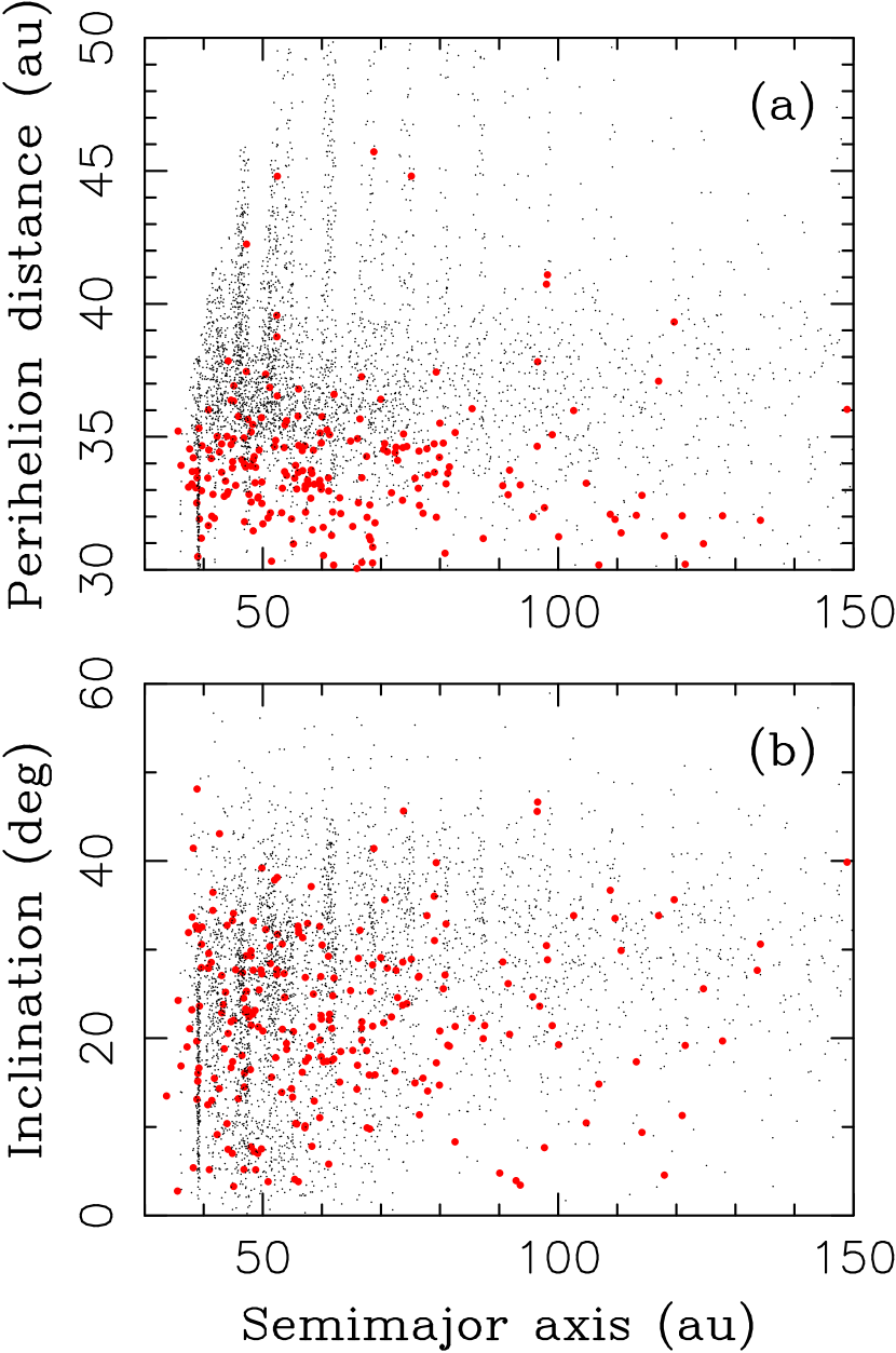
Figure 3: The source reservoir of Centaurs. We identified all modern-day Centaurs in the s30/100 simulation and plotted their orbits 1 Gyr ago (red dots). The small black dots show the model distribution of trans-Neptunian objects 1 Gyr ago.

We identified all objects that evolved onto Centaur orbits in our simulations and tracked their orbits back in time to establish their orbital histories. All these objects started in the original planetesimal disk below 30 au (Section 2). Figure 3 shows their orbits 1 Gyr ago when they resided in the trans-Neptunian region beyond 30 au. We find that 89% of Centaurs had Kuiper belt/scattered disk orbits with $a<5000$ au and 11% were in the Oort cloud ($a>5000$ au). For comparison, Nesvorný et al. (2017) found that 95% of ecliptic comets (orbital period $P<20$ yr and the Tisserand parameter with respect to Jupiter $2<T_{\rm J}<3$). evolved from orbits with $a<200$ au and 95% of Halley-type comets ($20<P<200$ yr, $T_{\rm J}<2$) evolved from the Oort cloud.

The source orbits of Centaurs show strong preference for $a<200$ au (85% of the total). Of these, 31% have $a<50$ au and 54% have $50<a<200$ au. In this sense, the scattered disk beyond 50 au is the main source of Centaurs, but the contribution from the classical/resonant Kuiper belt at $30<a<50$ au is also significant. For comparison, 20% of ecliptic comets come from $30<a<50$ au and 75% from $50<a<200$ au (Nesvorný et al. 2017). The preference for the scattered disk is therefore more pronounced for the ecliptic comets than for Centaurs. Also, 68% (76%) of Centaurs evolved from orbits with $q<35$ au ($q<36$ au) and $a<200$ au, which shows that the source orbits are typically at least marginally coupled to Neptune. This makes sense because the trans-Neptunian orbits with $q>36$ au are generally more stable and less often evolve to become planet crossing.

The fact that 11% of Centaurs evolved from the Oort cloud in our simulations could explain at least some the known very-high-inclination Centaurs (Gomes et al. 2015, Batygin & Brown 2016). OSSOS detected one Centaur with with $i=87^{\circ}$, $a=12.9$ au and $q=11.7$ au. This represents a $\sim$6% fraction of OSSOS Centaurs considered here. For comparison, orbits with $i>70^{\circ}$ represent only 0.6% of our model Centaurs detected by the OSSOS simulator. The probability of matching observations is thus roughly 1 in 10. Other sources of very-high-inclination Centaurs (Gomes et al. 2015, Batygin & Brown 2016) may be needed at this level of significance. A more stringent constraint would be obtained with a larger ensemble of Centaurs.

3.4 2060 Chiron and 29P/Schwassmann–Wachmann 1

Our dynamical model of Centaurs can be used to answer interesting questions about orbital evolution of specific objects. Here we illustrate these calculations for 2060 Chiron ($a=13.6$ au, $e=0.38$, $i=6.9^{\circ}$) and 29P/Schwassmann–Wachmann 1 (hereafter SW1; $a=5.99$ au, $e=0.044$, $i=9.4^{\circ}$). The nearly circular orbit of SW1 with the perihelion distance at $q=a(1-e)=5.72$ au and the aphelion distance at $Q=a(1+e)=6.25$ au is unusual among Centaurs; it does not intersect any planetary orbit. We may ask, for example, when SW1 evolved to its current orbit.

To answer this question, we select all simulated bodies with SW1-like orbits and calculate how long these bodies spent -on average and before arriving onto SW1-like orbits- with perihelion distance $q<6$ au and semimajor axis $a<7.5$ au. The answer is 38,000 yr. Using a typical SW1 production rate, we estimate that $\sim$4% of the SW1 mass would sublimate in 38,000 yr, thus eroding the SW1 diameter by $\sim$2 km (the SW1 diameter is estimated to be $\sim$50 km).

Another interesting question, with implications for the past activity of Chiron and SW1, is: “What is the probability that these objects had $q<3$ au (roughly the water ice sublimation radius) at any moment in the past?” Here we select all simulated bodies that reached the present orbit of Chiron and compute the fraction of these bodies that had $q<3$ au before reaching Chiron’s orbit. We find that the probability of Chiron having $q<3$ au in the past is only 7%. The same calculation for SW1 gives 11%. This shows that it is quite unlikely that any of these bodies experienced water-ice-sublimation-driven activity.

For comparison, all comets visited by spacecrafts had $q<1.6$ au when observations were made. In addition, from Nesvorný et al. (2013) we estimate that $\sim$80-90% of Jupiter Trojans had $q<3$ au before they were captured as Jupiter’s co-orbitals. Morbidelli et al. (2005) quoted similarly high probabilities in their capture model (e.g., 68% of Trojans reached $q<2$ au before capture). This suggests that targets of the NASA Lucy mission were significantly more altered by solar heating (and water ice sublimation) than Chiron and SW1.

4 Discussion

Recalibrating the number of planetesimals in the original disk from OSSOS Centaurs, we find that there were $(8\pm 3)\times 10^{9}$ planetesimals with $D>10$ km in the original outer disk. This implies only a minor adjustment of the population estimates given in Nesvorný (2018). For example, the inner scattered disk at $50<a<200$ au should contain $(2.0\pm 0.8)\times 10^{7}$ $D>10$ km bodies and the Oort cloud should contain $(5.0\pm 1.9)\times 10^{8}$ $D>10$ km comets. The error bars given above are standard 1$\sigma$ uncertainties that only take into account the number statistics of Centaurs detected by OSSOS. Additional uncertainties arise, for example, from the conversion between diameter and absolute magnitude.

So far we discussed the results from the s30/100 model, where Neptune was assumed to have migrated on an $e$-folding timescale $\tau_{1}=30$ Myr before the instability and $\tau_{2}=100$ Myr after the instability. The preference for these long migration timescales is explained in Nesvorný (2018). The results for s10/30 with $\tau_{1}=10$ Myr and $\tau_{2}=30$ Myr are similar, but we find that the inclination distribution of the biased s10/30 model is somewhat narrower (but non-rejectable). This is a consequence of shorter migration timescales in s10/30 that lead to somewhat smaller inclinations of orbits in the scattered disk.

The intrinsic orbit (Figure 1) and size distributions (Figure 2) of Centaurs inferred here represent an interesting prediction for the Large Synoptic Survey Telescope (LSST) observations. We find that $\simeq$90% and $\simeq$50% of Centaurs should have $a>20$ au and $a>25$ au, respectively. The median perihelion distance and median orbital inclination should be $\simeq$26 au and $\simeq$24^∘. The population of Centaurs is estimated to be $21,000\pm 8,000$ for $D>10$ km, $650\pm 250$ for $D>50$ km and $150\pm 60$ for $D>100$ km (estimates based on the size distribution shown in Figure 2; using $N(>\!\!D)=21,000(D/10)^{-2.1}$ would give $720\pm 280$ for $D>50$ km and $170\pm 70$ for $D>100$ km). The estimate for $D>100$ km is consistent with $120^{+90}_{-60}$ Centaurs with $H_{r}<8.66$ ($D>100$ km for a 6% albedo) from Lawler et al. (2018b).

model	$a_{{\rm N},0}$	$\tau_{1}$	$\tau_{2}$	$N_{\rm Pluto}$
	(au)	(Myr)	(Myr)
s10/30	24	10	30	2000
s30/100	24	30	100	4000

Table 1: A two stage migration of Neptune was adopted from Nesvorný & Vokrouhlický (2016): $\tau_{1}$ and $\tau_{2}$ define the $e$-folding exponential migration timescales during these stages, $a_{\rm N,0}$ denotes Neptune’s initial semimajor axis, and $N_{\rm Pluto}$ is the assumed initial number of Pluto-mass objects in the massive disk below 30 au. Neptune’s migration is grainy with these objects as needed to explain the observed proportion of resonant and non-resonant populations in the Kuiper belt.

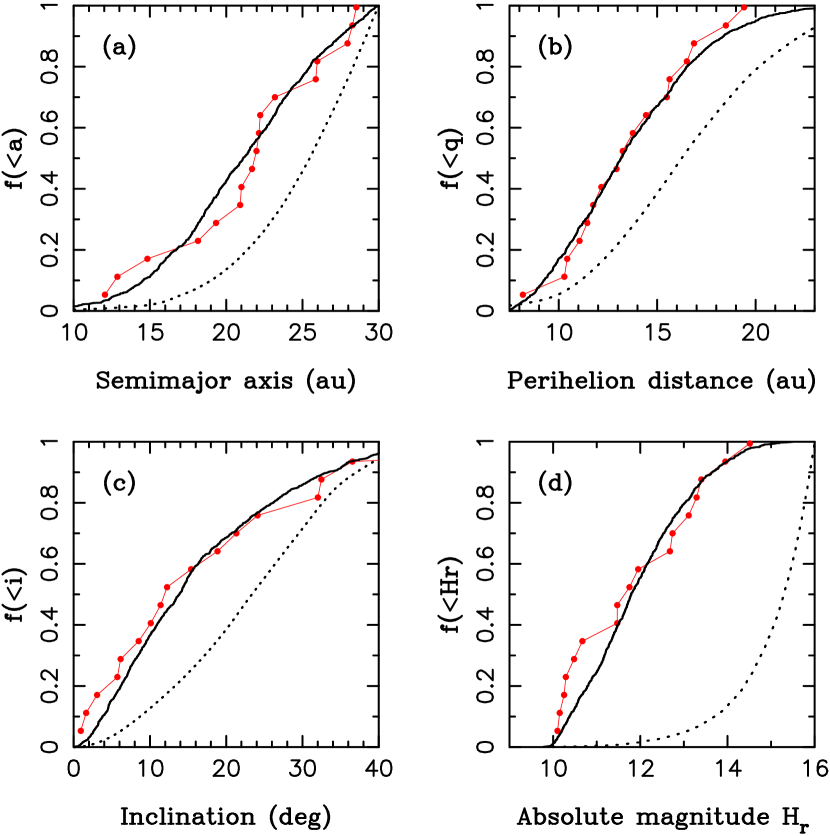
Figure 1: Comparison of the biased model distributions (solid lines) with OSSOS detections of Centaurs (connected red dots). Panels (a) to (d) show the semimajor axis, perihelion distance, inclination and absolute magnitude (fractional cumulative) distributions. The intrinsic distributions are shown as dotted lines. This result was obtained for the s30/100 model listed in Table 1.

Figure 2: The inferred size distribution of Centaurs. We extracted the size distribution of Jupiter Trojans from WISE (Grav et al. 2011), which is nearly complete down to $D=10$ km, and normalized it to 21,000 Centaurs with $D>10$ km (see section 3.2). The dashed line for $D<10$ km shows an extrapolated distribution $N(>\!\!D)=21,000\times(D/10\,{\rm km})^{-2.1}$. The size range of Centaurs detected by OSSOS is indicated by arrows.

References

- Alexandersen et al. (2016) Alexandersen, M., Gladman, B., Kavelaars, J. J., et al. 2016, VizieR Online Data Catalog, 515,
- Bannister et al. (2018) Bannister, M. T., Gladman, B. J., Kavelaars, J. J., et al. 2018, ApJS, 236, 18
- Batygin & Brown (2016) Batygin, K., & Brown, M. E. 2016, ApJ, 833, L3
- Bauer et al. (2013) Bauer, J. M., Grav, T., Blauvelt, E., et al. 2013, ApJ, 773, 22
- Bernstein et al. (2004) Bernstein, G. M., Trilling, D. E., Allen, R. L., et al. 2004, AJ, 128, 1364
- Brasser & Morbidelli (2013) Brasser, R., & Morbidelli, A. 2013, Icarus, 225, 40
- Cabral et al. (2019) Cabral, N., Guilbert-Lepoutre, A., Fraser, W. C., et al. 2019, A&A, 621, A102
- Di Sisto & Brunini (2007) Di Sisto, R. P., & Brunini, A. 2007, Icarus, 190, 224
- Duffard et al. (2014) Duffard, R., Pinilla-Alonso, N., Santos-Sanz, P., et al. 2014, A&A, 564, A92
- Duncan & Levison (1997) Duncan, M. J., & Levison, H. F. 1997, Science, 276, 1670
- Emery et al. (2015) Emery, J. P., Marzari, F., Morbidelli, A., French, L. M., & Grav, T. 2015, Asteroids IV, 203
- Fraser et al. (2014) Fraser, W. C., Brown, M. E., Morbidelli, A., Parker, A., & Batygin, K. 2014, ApJ, 782, 100
- Gladman et al. (2008) Gladman, B., Marsden, B. G., & Vanlaerhoven, C. 2008, The Solar System Beyond Neptune, 43
- Gomes et al. (2015) Gomes, R. S., Soares, J. S., & Brasser, R. 2015, Icarus, 258, 37
- Grav et al. (2011) Grav, T., Mainzer, A. K., Bauer, J., et al. 2011, ApJ, 742, 40
- Hahn & Malhotra (2005) Hahn, J. M., & Malhotra, R. 2005, AJ, 130, 2392
- Lawler et al. (2018) Lawler, S. M., Kavelaars, J. J., Alexandersen, M., et al. 2018a, Frontiers in Astronomy and Space Sciences, 5, 14
- Lawler et al. (2018) Lawler, S. M., Shankman, C., Kavelaars, J. J., et al. 2018b, AJ, 155, 197
- Levison, & Duncan (1994) Levison, H. F., & Duncan, M. J. 1994, Icarus, 108, 18
- Levison & Duncan (1997) Levison, H. F., & Duncan, M. J. 1997, Icarus, 127, 13
- Levison et al. (2008) Levison, H. F., Morbidelli, A., Vokrouhlický, D., & Bottke, W. F. 2008, AJ, 136, 1079
- Morbidelli et al. (2005) Morbidelli, A., Levison, H. F., Tsiganis, K., & Gomes, R. 2005, Nature, 435, 462
- Morbidelli et al. (2009) Morbidelli, A., Levison, H. F., Bottke, W. F., Dones, L., & Nesvorný, D. 2009, Icarus, 202, 310
- Nesvorný (2015) Nesvorný, D. 2015, AJ, 150, 73
- Nesvorný (2018) Nesvorný, D. 2018, ARA&A, 56, 137
- Nesvorný & Morbidelli (2012) Nesvorný, D., & Morbidelli, A. 2012, AJ, 144, 117
- Nesvorný & Vokrouhlický (2016) Nesvorný, D., & Vokrouhlický, D. 2016, ApJ, 825, 94
- Nesvorný, & Vokrouhlický (2019) Nesvorný, D., & Vokrouhlický, D. 2019, Icarus, 331, 49
- Nesvorný et al. (2013) Nesvorný, D., Vokrouhlický, D., & Morbidelli, A. 2013, ApJ, 768, 45
- Nesvorný et al. (2017) Nesvorný, D., Vokrouhlický, D., Dones, L., et al. 2017, ApJ, 845, 27
- Petit et al. (2011) Petit, J.-M., Kavelaars, J. J., Gladman, B. J., et al. 2011, AJ, 142, 131
- Pirani et al. (2018) Pirani, S., Johansen, A., Bitsch, B., Mustill, A. J., & Turrini, D. 2018, AAS/Division for Planetary Sciences Meeting Abstracts #50, 50, 200.01D
- Shankman et al. (2013) Shankman, C., Gladman, B. J., Kaib, N., Kavelaars, J. J., & Petit, J. M. 2013, ApJ, 764, L2
- Shankman et al. (2016) Shankman, C., Kavelaars, J., Gladman, B. J., et al. 2016, AJ, 151, 31
- Singer et al. (2019) Singer, K. N., McKinnon, W. B., Gladman, B., et al. 2019, arXiv:1902.10795
- Volk & Malhotra (2008) Volk, K., & Malhotra, R. 2008, ApJ, 687, 714
- Volk & Malhotra (2013) Volk, K., & Malhotra, R. 2013, Icarus, 224, 66