Emergence of conformal symmetry in quantum spin chains:
anti-periodic boundary conditions and supersymmetry

Abstract

Universal properties of a critical quantum spin chain are encoded in the underlying conformal field theory (CFT). This underlying CFT is fully characterized by its conformal data. We propose a method to extract the conformal data from a critical quantum spin chain with both periodic and anti-periodic boundary conditions (PBC and APBC) based on low-energy eigenstates, generalizing previous work on spin chains with only PBC. First, scaling dimensions and conformal spins are extracted from the energies and momenta of the eigenstates. Second, the Koo-Saleur formula of lattice Virasoro generators is generalized to APBC and used to identify conformal towers. Third, local operators and string operators on the lattice are identified with CFT operators with PBC and APBC, respectively. Finally, operator product expansion coefficients are extracted by computing matrix elements of lattice primary operators in the low-energy subspaces with PBC and APBC. To go beyond exact diagonalization, tensor network methods based on periodic uniform matrix product states are used. We illustrate our approach with critical and tricritical Ising quantum spin chains. In the latter case, we propose lattice operators that correspond to supervirasoro generators and verify their action on low-energy eigenstates. In this way we explore the emergence of superconformal symmetry in the quantum spin chain.

I Introduction

Understanding the universality class Wilson and Kogut (1974) of a critical quantum system chain is an important problem in modern physics. At long distances, a critical quantum system is often described by a conformal field theory (CFT) Belavin et al. (1984); Friedan et al. (1984), which is in turn specified by the conformal data.

Given a critical quantum spin Hamiltonian $H$ in 1+1 dimensions, an ambitious, yet challenging task is to extract the conformal data for the emergent CFT. One method is based on the operator-state correspondence Belavin et al. (1984); Friedan et al. (1984); Ginsparg (1988); Henkel (1999); Di Francesco et al. (2012). This refers to the fact that in a 1+1 dimensional CFT, every state $|\psi^{\textsl{\tiny CFT}}_{\alpha}\rangle$ on the circle is in one to one correspondence with a scaling operator $\psi^{\textsl{\tiny CFT}}_{\alpha}$ (an operator that transforms covariantly under scale transformations and rotations of the plane). Each low energy eigenstate $|\psi_{\alpha}\rangle$ of the lattice Hamiltonian $H$ with periodic boundary conditions (PBC) is an approximate lattice realization of the CFT state $|\psi^{\textsl{\tiny CFT}}_{\alpha}\rangle$. Conformal data can then be extracted from matrix elements of certain lattice operators $\langle\psi_{\alpha}|O|\psi_{\beta}\rangle$ Cardy (1984a); Blöte et al. (1986); Affleck (1986); Cardy (1986a); Koo and Saleur (1994); Milsted and Vidal (2017); Zou et al. (2019) and extrapolation of the results to the thermodynamic limit. Moreover, there are recently proposed numerical methods Zou et al. (2018) to efficiently diagonalize all low energy eigenstates of a critical quantum spin chain with PBC up to several hundreds of spins. This significantly improves the accuracy of the extrapolation to large system sizes.

However, PBC only allows access to a subset of scaling operators Cardy (1984b, 1989). For the rest, other boundary conditions are needed, such as antiperiodic boundary conditions (APBC) or, more generally, twisted boundary conditions. Furthermore, in case the CFT has an extended symmetry, the representations of the full symmetry group may involve mixing boundary conditions. In particular, when the conformal symmetry is enhanced by supersymmetry Friedan et al. (1984, 1985), which transforms bosons into fermions, the fermionic excitations (appearing in the APBC sector) are needed to form a representation of the superconformal algebra.

In this paper, we generalize the method of Refs. Zou et al. (2018, 2019) to critical spins chains with APBC (more general twisted boundary conditions can be addressed in a similar way). We propose a systematic way of extracting complete conformal data involving scaling operators in the APBC. The efficient diagonalization method of low energy eigenstates is also generalized to the APBC. As applications, we then extract accurate conformal data for two models with APBC, namely the Ising model and a tricritical Ising (TCI) model O’Brien and Fendley (2018) due to O’Brien and Fendley. For the latter case the APBC excitations enable us to study the emergent superconformal symmetry.

More specifically, given a critical quantum spin chain with PBC and APBC, we first diagonalize the low-energy eigenstates and identify each eigenstate on the lattice with a CFT scaling operator in the continuum. In particular, primary states can their conformal towers are identified for both boundary conditions. Then we find lattice operators that correspond to CFT primary operators in the continuum limit. All OPE coefficients involving primary operators can then be extracted. Furthermore, in the case where the conformal symmetry is enhanced by supersymmetry, such as the TCI model, we can identify generators of the extended algebra (supervirasoro algebra) on the lattice. By studying the action of supervirasoro generators on the low-energy subspace, we can identify supervirasoro primary states and supervirasoro conformal towers.

This paper is organized as following. In section II we review conformal data and operator-state correspondence of 1+1 dimensional CFT and previous work on extracting conformal data from a critical quantum spin chain. In section III we define APBC for spin chains and APBC for CFT and discuss their relations. In section IV we propose a systematic way of extracting conformal data based on the low energy spectrum of the spin chain with APBC. In section V we generalize the efficient diagonalization of low energy eigenstates of a critical quantum spin chain from PBC to APBC. In section VI, we extract conformal data from the Ising model. In section VII, we consider the more complicated TCI model and extract its conformal data. In section VIII, we construct lattice representations of superconformal generators that connect eigenstates in PBC and APBC and verify the superconformal structure of low energy excitations.

II Conformal data and its extraction

In this section, we review some basic properties of conformal field theories Belavin et al. (1984); Friedan et al. (1984); Ginsparg (1988); Henkel (1999); Di Francesco et al. (2012) and summarize the way of extracting conformal data based on the operator-state correspondence in PBC. These results are to be generalized to APBC in this paper.

II.1 Conformal data

In 1+1 dimensions, a conformal field theory consists of a set of scaling operators $\psi^{\textsl{\tiny CFT}}_{\alpha}(z,\bar{z})$, where $z=x^{0}+ix^{1}$ and $\bar{z}=x^{0}-ix^{1}$ are complex coordinates. Each scaling operator has a scaling dimension $\Delta^{\textsl{\tiny CFT}}_{\alpha}$ and a conformal spin $s^{\textsl{\tiny CFT}}_{\alpha}$, which describe how the scaling operators transform under dilations and rotations, respectively,

$$z\rightarrow z^{\prime} = \lambda z,\leavevmode\nobreak\ \leavevmode\nobreak\ \leavevmode\nobreak\ \leavevmode\nobreak\ \psi^{\textsl{\tiny CFT}}_{\alpha}(z,\bar{z})\rightarrow\lambda^{-\Delta^{\textsl{\tiny CFT}}_{\alpha}}\psi^{\textsl{\tiny CFT}}_{\alpha}(z^{\prime},\bar{z}^{\prime})$$ (1)

$$z\rightarrow z^{\prime} = e^{i\theta}z,\leavevmode\nobreak\ \leavevmode\nobreak\ \psi^{\textsl{\tiny CFT}}_{\alpha}(z,\bar{z})\rightarrow e^{-i\theta s^{\textsl{\tiny CFT}}_{\alpha}}\psi^{\textsl{\tiny CFT}}_{\alpha}(z^{\prime},\bar{z}^{\prime}),$$ (2)

where $\lambda>0$ and $0\leq\theta<2\pi$. All two point correlation functions in the CFT are determined by $(\Delta^{\textsl{\tiny CFT}}_{\alpha},s^{\textsl{\tiny CFT}}_{\alpha})$.

Scaling operators are organized into conformal towers, with a primary field $\phi^{\textsl{\tiny CFT}}_{\alpha}$ in each conformal tower and the descendant fields of this primary field. The descendant fields are related to the primary field by Virasoro generators $L^{\textsl{\tiny CFT}}_{n}$ and $\bar{L}^{\textsl{\tiny CFT}}_{n}$ ($n\in\mathbb{Z}$) which act as ladder operators. They generate conformal transformations and satisfy the Virasoro algebra

$$[ L^{\textsl{\tiny CFT}}_{n},L^{\textsl{\tiny CFT}}_{m}]=(n-m)L^{\textsl{\tiny CFT}}_{n+m}+\frac{c^{\textsl{\tiny CFT}}}{12}n(n^{2}-1)\delta_{n+m,0}$$ (3)

$$[ \bar{L}^{\textsl{\tiny CFT}}_{n},\bar{L}^{\textsl{\tiny CFT}}_{m}]=(n-m)\bar{L}^{\textsl{\tiny CFT}}_{n+m}+\frac{c^{\textsl{\tiny CFT}}}{12}n(n^{2}-1)\delta_{n+m,0}$$ (4)

$$[ L^{\textsl{\tiny CFT}}_{n},\bar{L}^{\textsl{\tiny CFT}}_{m}]=0,$$ (5)

where $c^{\textsl{\tiny CFT}}$ is the central charge that is a part of the conformal data. In particular, $D^{\textsl{\tiny CFT}}=L^{\textsl{\tiny CFT}}_{0}+\bar{L}^{\textsl{\tiny CFT}}_{0}$ and $R^{\textsl{\tiny CFT}}=L^{\textsl{\tiny CFT}}_{0}-\bar{L}^{\textsl{\tiny CFT}}_{0}$ generate dilations and rotations. Scaling operators $\psi^{\textsl{\tiny CFT}}_{\alpha}(0,0)$ are eigenvectors of $D^{\textsl{\tiny CFT}}$ and $R^{\textsl{\tiny CFT}}$, with eigenvalues $\Delta^{\textsl{\tiny CFT}}_{\alpha}$ and $s^{\textsl{\tiny CFT}}_{\alpha}$,

$$[D^{\textsl{\tiny CFT}},\psi^{\textsl{\tiny CFT}}_{\alpha}(0,0)]=\Delta^{\textsl{\tiny CFT}}_{\alpha}\psi^{\textsl{\tiny CFT}}_{\alpha}(0,0)$$ (6)

$$[R^{\textsl{\tiny CFT}},\psi^{\textsl{\tiny CFT}}_{\alpha}(0,0)]\,=s^{\textsl{\tiny CFT}}_{\alpha}\psi^{\textsl{\tiny CFT}}_{\alpha}(0,0).$$ (7)

Virasoro generators $L^{\textsl{\tiny CFT}}_{n}$ and $\bar{L}^{\textsl{\tiny CFT}}_{n}$ with $n<0$ are raising operators with respect to dilations – they raise the scaling dimension by $|n|$, while those with $n>0$ lower the scaling dimension by $n$,

$$[D^{\textsl{\tiny CFT}},[L^{\textsl{\tiny CFT}}_{n},\psi^{\textsl{\tiny CFT}}_{\alpha}(0,0)]]=(\Delta^{\textsl{\tiny CFT}}_{\alpha}-n)[L^{\textsl{\tiny CFT}}_{n},\psi^{\textsl{\tiny CFT}}_{\alpha}(0,0)]$$ (8)

$$[D^{\textsl{\tiny CFT}},[\bar{L}^{\textsl{\tiny CFT}}_{n},\psi^{\textsl{\tiny CFT}}_{\alpha}(0,0)]]=(\Delta^{\textsl{\tiny CFT}}_{\alpha}-n)[\bar{L}^{\textsl{\tiny CFT}}_{n},\psi^{\textsl{\tiny CFT}}_{\alpha}(0,0)].$$ (9)

Primary fields are those whose scaling dimensions cannot be lowered

$$[L^{\textsl{\tiny CFT}}_{n},\phi^{\textsl{\tiny CFT}}_{\alpha}(0,0)]=0,[\bar{L}^{\textsl{\tiny CFT}}_{n},\phi^{\textsl{\tiny CFT}}_{\alpha}(0,0)]=0\leavevmode\nobreak\ \leavevmode\nobreak\ (n>0).$$ (10)

Descendant fields in a conformal tower can be obtained by applying raising operators $L^{\textsl{\tiny CFT}}_{n},\bar{L}^{\textsl{\tiny CFT}}_{n}$ ($n<0$) to the primary field of that tower.

The scaling operators form an associative algebra, the operator product expansion (OPE), which relates the product of two scaling operators to a linear superposition of scaling operators. Three and higher point correlation functions are determined by the OPE. It turns out the OPE is completely characterized by the coefficients $C^{\textsl{\tiny CFT}}_{\alpha\beta\gamma}$ involving primary fields Belavin et al. (1984); Friedan et al. (1984); Cardy (1986a). Therefore, we conclude that the conformal data consists of $\{\Delta^{\textsl{\tiny CFT}}_{\alpha},s^{\textsl{\tiny CFT}}_{\alpha},C^{\textsl{\tiny CFT}}_{\alpha\beta\gamma}\}$ for primary fields and the central charge $c^{\textsl{\tiny CFT}}$.

II.2 Operator-state correspondence and extraction of conformal data from a CFT on the cylinder

The CFT can be put on a cylinder with a compactified spatial direction $x\in[0,L)$ and an uncompactified time direction $\tau\in(-\infty,\infty)$. The Hamiltonian and momentum are the integrals of the Hamiltonian and momentum density $h^{\textsl{\tiny CFT}}(x)$ and $p^{\textsl{\tiny CFT}}(x)$ on the time slice $\tau=0$,

$$H^{\textsl{\tiny CFT}} = \int_{0}^{L}dx\,h^{\textsl{\tiny CFT}}(x)$$ (11)

$$P^{\textsl{\tiny CFT}} = \int_{0}^{L}dx\,p^{\textsl{\tiny CFT}}(x).$$ (12)

They are related to the generators of dilations and rotations of the CFT on the complex plane by

$$H^{\textsl{\tiny CFT}} = \frac{2\pi}{L}\left(L^{\textsl{\tiny CFT}}_{0}+\bar{L}^{\textsl{\tiny CFT}}_{0}-\frac{c}{12}\right)$$ (13)

$$P^{\textsl{\tiny CFT}} = \frac{2\pi}{L}\left(L^{\textsl{\tiny CFT}}_{0}-\bar{L}^{\textsl{\tiny CFT}}_{0}\right).$$ (14)

The operator-state correspondence Belavin et al. (1984); Friedan et al. (1984); Cardy (1984a); Blöte et al. (1986) says that all simultaneous eigenstates $|\psi^{\textsl{\tiny CFT}}_{\alpha}\rangle$ of $H^{\textsl{\tiny CFT}}$ and $P^{\textsl{\tiny CFT}}$ are in one to one correspondence with scaling operators $\psi^{\textsl{\tiny CFT}}_{\alpha}$. The energy and momentum are thus related to scaling dimensions and conformal spins by

$$E^{\textsl{\tiny CFT}}_{\alpha} = \frac{2\pi}{L}\left(\Delta^{\textsl{\tiny CFT}}_{\alpha}-\frac{c}{12}\right)$$ (15)

$$P^{\textsl{\tiny CFT}}_{\alpha} = \frac{2\pi}{L}s^{\textsl{\tiny CFT}}_{\alpha}.$$ (16)

Virasoro generators can be expressed as Fourier modes of $h(x)$ and $p(x)$. In particular, the Fourier modes of $h^{\textsl{\tiny CFT}}(x)$,

$$H^{\textsl{\tiny CFT}}_{n}\equiv\frac{L}{2\pi}\int_{0}^{L}dx\,h^{\textsl{\tiny CFT}}(x)e^{inx2\pi/L}$$ (17)

equal a linear combination of Virasoro generators Koo and Saleur (1994); Milsted and Vidal (2017),

$$H^{\textsl{\tiny CFT}}_{n}=L^{\textsl{\tiny CFT}}_{n}+\bar{L}^{\textsl{\tiny CFT}}_{-n}-\frac{c^{\textsl{\tiny CFT}}}{12}\delta_{n,0}.$$ (18)

The central charge can be computed by

$$c^{\textsl{\tiny CFT}}=2|\langle T^{\textsl{\tiny CFT}}|H^{\textsl{\tiny CFT}}_{-2}|0^{\textsl{\tiny CFT}}\rangle|^{2},$$ (19)

where $|0^{\textsl{\tiny CFT}}\rangle$ is the ground state of the CFT and the state $|T^{\textsl{\tiny CFT}}\rangle$ corresponds to the stress tensor of the CFT.

Primary fields $\phi^{\textsl{\tiny CFT}}_{\alpha}$ correspond to primary states $|\phi^{\textsl{\tiny CFT}}_{\alpha}\rangle$, which are characterized by Milsted and Vidal (2017); Zou et al. (2018)

$$L^{\textsl{\tiny CFT}}_{n}|\phi^{\textsl{\tiny CFT}}_{\alpha}\rangle=0,\bar{L}^{\textsl{\tiny CFT}}_{n}|\phi^{\textsl{\tiny CFT}}_{\alpha}\rangle=0\leavevmode\nobreak\ \leavevmode\nobreak\ (n>0).$$ (20)

Note that the Virasoro algebra Eq. (3) implies that the above equalities hold for all $n>0$ if they hold for $n=1,2$, since other generators can be obtained by commutators of those with $n=1,2$.

The two Virasoro generators $L^{\textsl{\tiny CFT}}_{-n}$ and $\bar{L}^{\textsl{\tiny CFT}}_{n}$ in $H^{\textsl{\tiny CFT}}_{n}$, Eq. (18), raise scaling dimensions and lower scaling dimensions respectively for $n\neq 0$. Therefore, primary states can be alternatively defined as

$$P^{\textsl{\tiny CFT}}_{\phi_{\alpha}}H^{\textsl{\tiny CFT}}_{n}|\phi^{\textsl{\tiny CFT}}_{\alpha}\rangle=0\leavevmode\nobreak\ \leavevmode\nobreak\ (n=\pm 1,\pm 2),$$ (21)

where $P^{\textsl{\tiny CFT}}_{\phi_{\alpha}}$ is a projector onto the subspace spanned by states whose scaling dimension is smaller than that of $\phi^{\textsl{\tiny CFT}}_{\alpha}$.

Descendant states corresponding to descendant fields can be created by acting with $L^{\textsl{\tiny CFT}}_{n}$,$\bar{L}^{\textsl{\tiny CFT}}_{n}$ ($n<0$) on primary states.

OPE coefficients of primary fields are related to matrix elements of primary operators,

$$\langle\phi^{\textsl{\tiny CFT}}_{\alpha}|\phi^{\textsl{\tiny CFT}}_{\beta}(x=0)|\phi^{\textsl{\tiny CFT}}_{\gamma}\rangle=\left(\frac{2\pi}{L}\right)^{\Delta^{\textsl{\tiny CFT}}_{\beta}}C^{\textsl{\tiny CFT}}_{\alpha\beta\gamma}.$$ (22)

Translation invariance of the eigenstates allow us to express the OPE coefficients in terms of the Fourier mode of the CFT operator,

$$\langle\phi^{\textsl{\tiny CFT}}_{\alpha}|\phi^{\textsl{\tiny CFT},s_{\alpha}-s_{\gamma}}_{\beta}|\phi^{\textsl{\tiny CFT}}_{\gamma}\rangle=\left(\frac{2\pi}{L}\right)^{\Delta^{\textsl{\tiny CFT}}_{\beta}}C^{\textsl{\tiny CFT}}_{\alpha\beta\gamma},$$ (23)

where the Fourier mode of any CFT operaror is defined as

$$\mathcal{O}^{\textsl{\tiny CFT},s}\equiv\frac{1}{L}\int_{0}^{L}dx\,\mathcal{O}^{\textsl{\tiny CFT}}(x)e^{-isx2\pi/L}.$$ (24)

II.3 Extraction of conformal data from a spin chain

Given a critical quantum spin chain $H=\sum_{j}h_{j}$ with PBC, it has been shown Cardy (1984a); Blöte et al. (1986); Affleck (1986); Cardy (1986a); Koo and Saleur (1994); Milsted and Vidal (2017); Zou et al. (2019) that all conformal data can be extracted from appropriate matrix elements of lattice operators in the low energy eigenstates, which we now review. We will see that the formulas are analogous to Eqs. (15)-(22).

At low energies, each eigenstate of $H$ is in one to one correspondence with a CFT state,

$$|\psi_{\alpha}\rangle\sim|\psi^{\textsl{\tiny CFT}}_{\alpha}\rangle.$$ (25)

Denote the total number of sites as $N$. We can think of $N$ as analogous to the circumference $L$ of the cylinder. The energy and momentum $E_{\alpha}$ and $P_{\alpha}$ are related to $\Delta^{\textsl{\tiny CFT}}_{\alpha}$ and $s^{\textsl{\tiny CFT}}_{\alpha}$ by Cardy (1984a); Blöte et al. (1986); Affleck (1986); Cardy (1986a, b)

$$E_{\alpha} = NA+\frac{B}{N}\left(\Delta^{\textsl{\tiny CFT}}_{\alpha}-\frac{c}{12}\right)+o(N^{-1})$$ (26)

$$P_{\alpha} = \frac{2\pi}{N}s^{\textsl{\tiny CFT}}_{\alpha},$$ (27)

where $A,B$ are non-universal constants related to the lattice model. At sufficiently large sizes, the subleading correction $o(N^{-1})$ is negligible. The constants $A$ and $B$ can be numerically estimated by using the fact that scaling dimensions of the ground state and the stress tensor state are always $\Delta_{I}=0$, $\Delta_{T}=2$ in a unitary CFT. $A$ is the ground state energy density in the thermodynamic limit and

$$B\approx\frac{N}{2}(E_{T}-E_{0}).$$ (28)

We can then extract the scaling dimensions and conformal spins as

$$\Delta_{\alpha} = 2\frac{E_{\alpha}-E_{0}}{E_{T}-E_{0}}$$ (29)

$$s_{\alpha} = \frac{N}{2\pi}P_{\alpha}.$$ (30)

Notice that $\Delta_{\alpha}$ and $\Delta^{\textsl{\tiny CFT}}_{\alpha}$ differ by finite-size corrections, but $s_{\alpha}=s^{\textsl{\tiny CFT}}_{\alpha}$ (up to periodicity $N$) is exact because momenta are quantized. To obtain a more accurate approximation to $\Delta^{\textsl{\tiny CFT}}_{\alpha}$, we can compute $\Delta_{\alpha}$ as a function of $N$ at finite sizes and extrapolate to $N\rightarrow\infty$ (the thermodynamic limit).

Furthermore, a local lattice operator $\mathcal{O}$ can be identified with a CFT operator $\mathcal{O}^{\textsl{\tiny CFT}}$ Cardy (1986a); Zou et al. (2019)

$$\mathcal{O}\sim\mathcal{O}^{\textsl{\tiny CFT}}=\sum_{\alpha}a_{\alpha}\psi^{\textsl{\tiny CFT}}_{\alpha},$$ (31)

where $\psi^{\textsl{\tiny CFT}}_{\alpha}$ are scaling operators. In general, the expansion Eq. (31) involves infinite scaling operators with arbitrarily large scaling dimensions. However, we will work with a truncated expansion to some maximal scaling dimension $\Delta^{\textsl{\tiny CFT}}$. To compare a lattice operatr $\mathcal{O}$ with a CFT operator $\mathcal{O}^{\textsl{\tiny CFT}}$, we first define Fourier modes of the lattice operator ,

$$\mathcal{O}^{s}\equiv\frac{1}{N}\sum_{j=1}^{N}e^{-isj2\pi/N}\mathcal{O}_{j}.$$ (32)

They connect states with conformal spin $s_{\alpha}$ to states with conformal spin $s_{\alpha}+s$. The coefficients $a_{\alpha}$ can be obtained by minimizing the cost function Zou et al. (2019)

$$f^{\mathcal{O}}(\{a_{\alpha}\})=\sum_{\beta}|\langle\psi_{\beta}|\mathcal{O}^{s_{\beta}}|0\rangle-\langle\psi^{\textsl{\tiny CFT}}_{\beta}|\mathcal{O}^{\textsl{\tiny CFT},{s_{\beta}}}|0^{\textsl{\tiny CFT}}\rangle|^{2}$$ (33)

for some subset of low energy eigenstates $\{|\psi_{\beta}\rangle\}$. Note that the CFT matrix elements $\langle\psi^{\textsl{\tiny CFT}}_{\beta}|\mathcal{O}^{\textsl{\tiny CFT},{s_{\beta}}}|0^{\textsl{\tiny CFT}}\rangle$ can be computed as a function of scaling dimensions, conformal spins and the central charge Zou et al. (2019). Because there are finite-size corrections, the cost function is typically non-vanishing at finite $N$. An estimation of the coefficient $a_{\alpha}$ in the thermodynamic limit is obtained by an extrapolation of the finite-size data.

In particular, the lattice Hamiltonian density $h_{j}$ corresponds to the CFT Hamiltonian density $h^{\textsl{\tiny CFT}}(x)$ (up to a normalization factor and a constant shift), whose Fourier modes are linear combinations of Virasoro generators Koo and Saleur (1994); Read and Saleur (2007); Dubail et al. (2010); Vasseur et al. (2012); Gainutdinov et al. (2013); Gainutdinov and Vasseur (2013); Bondesan et al. (2015). Therefore,

$$H_{n}\equiv\frac{N}{B}\sum_{j=1}^{N}h_{j}e^{inj2\pi/N}\sim H^{\textsl{\tiny CFT}}_{n}.$$ (34)

Denote $P_{\phi_{\alpha}}$ the projector onto the subspace spanned by eigenstates whose energies are lower than that of $|\phi_{\alpha}\rangle$. Then, analogous to Eq. (21), primary states can be identified by the condition Milsted and Vidal (2017); Zou et al. (2018) that

$$P_{\phi_{\alpha}}H_{n}|\phi_{\alpha}\rangle=0\leavevmode\nobreak\ \leavevmode\nobreak\ (n=\pm 1,\pm 2)$$ (35)

in the thermodynamic limit. Other eigenstates can be approximately obtained by acting with $H_{n}\leavevmode\nobreak\ (n\neq 0)$ on the primary states, proceeding in analogy with the CFT.

An estimate $c$ of the central charge $c^{\textsl{\tiny CFT}}$ is obtained from

$$c=2|\langle T|H_{-2}|0\rangle|^{2},$$ (36)

analogous to Eq. (19). Again, a suitable extrapolation to the thermodynamic limit wii be used.

The identification Eq. (31) allows us to find a lattice operator $\mathcal{O}_{\phi_{\beta}}$ corresponding to the primary operator $\phi^{\textsl{\tiny CFT}}_{\beta}$ by inverting the linear expansion. The OPE coefficients $C^{\textsl{\tiny CFT}}_{\alpha\beta\gamma}$ can be extracted approximately from Cardy (1986a); Zou et al. (2019)

$$C_{\alpha\beta\gamma}=\left(\frac{2\pi}{N}\right)^{-\Delta_{\beta}}\langle\phi_{\alpha}|\mathcal{O}_{\phi_{\beta},j=0}|\phi_{\gamma}\rangle.$$ (37)

Due to translation invariance, the above matrix elements can also be computed by

$$C_{\alpha\beta\gamma}=\left(\frac{2\pi}{N}\right)^{-\Delta_{\beta}}\langle\phi_{\alpha}|\mathcal{O}^{s_{\alpha}-s_{\gamma}}_{\phi_{\beta}}|\phi_{\gamma}\rangle,$$ (38)

analogous to Eq. (23). Again, $C^{\textsl{\tiny CFT}}_{\alpha\beta\gamma}$ can be obtained by extrapolating $C_{\alpha\beta\gamma}$ to the thermodynamic limit.

In order to extrapolate accurate conformal data in the thermodynamic limit, it is essential to obtain energy eigenstates for a series of system sizes $N$ that are sufficiently large, such that finite-size corrections are small. To go beyond exact diagonalization, we will use a tensor network method based on matrix product states White (1992); Fannes et al. (1992); Rommer and Östlund (1997); Vidal (2004, 2007); Degli et al. (2004); Tagliacozzo et al. (2008); Xavier (2010); Stojevic et al. (2015); Schollwöck (2011). It has been shown Pirvu et al. (2011, 2012); Zou et al. (2018) that the tensor network method can be applied to obtain any energy eigenstate with sufficiently low energy for system sizes $N$ far beyond the reach of exact diagonalization, see section V.

We conclude this section with Table 1 that summarizes the correspondence between lattice objects and CFT objects for the PBC.

CFT	Lattice (at low energies)
Energy/momentum eigenstate $|\psi^{\textsl{\tiny CFT}}_{\alpha}\rangle$	Energy/momentum eigenstate $|\psi_{\alpha}\rangle$
Primary state $|\phi^{\textsl{\tiny CFT}}_{\alpha}\rangle$	Primary state $|\phi_{\alpha}\rangle$
Energy $E^{\textsl{\tiny CFT}}_{\alpha}=\frac{2\pi}{L}(\Delta^{\textsl{\tiny CFT}}_{\alpha}-{c^{\textsl{\tiny CFT}}}/{12})$	Energy $E_{\alpha}\approx NA+\frac{B}{2\pi}E^{\textsl{\tiny CFT}}_{\alpha}$ (Eq. (26))
Momentum $P^{\textsl{\tiny CFT}}_{\alpha}=\frac{2\pi}{L}s^{\textsl{\tiny CFT}}_{\alpha}$	Momentum $P_{\alpha}=P^{\textsl{\tiny CFT}}_{\alpha}$ (Eq. (27))
Local operator $\mathcal{O}^{\textsl{\tiny CFT}}=\sum_{\alpha}a_{\alpha}\psi^{\textsl{\tiny CFT}}_{\alpha}$	Local operator $\mathcal{O}$
Fourier mode $\mathcal{O}^{\textsl{\tiny CFT},s}$ (Eq. (24))	Fourier mode $\mathcal{O}^{s}$ (Eq. (32))
$H^{\textsl{\tiny CFT}}_{n}=L^{\textsl{\tiny CFT}}_{n}+\bar{L}^{\textsl{\tiny CFT}}_{-n}-{c^{\textsl{\tiny CFT}}}/{12}\delta_{n,0}$	$H_{n}$ (Eq. (34))
Primary operator $\phi^{\textsl{\tiny CFT}}_{\beta}$	Operator $\mathcal{O}_{\phi_{\beta}}$
$C^{\textsl{\tiny CFT}}_{\alpha\beta\gamma}=(2\pi/L)^{-\Delta^{\textsl{\tiny CFT}}_{\beta}}\langle\phi^{\textsl{\tiny CFT}}_{\alpha}|\phi^{\textsl{\tiny CFT},s_{\alpha}-s_{\gamma}}_{\beta}|\phi^{\textsl{\tiny CFT}}_{\gamma}\rangle$	$C_{\alpha\beta\gamma}=(2\pi/N)^{-\Delta_{\beta}}\langle\phi_{\alpha}|\mathcal{O}^{s_{\alpha}-s_{\gamma}}_{\phi_{\beta}}|\phi_{\gamma}\rangle\approx C^{\textsl{\tiny CFT}}_{\alpha\beta\gamma}$

Table 1: Correspondence of lattice objects and CFT objects. The ”$\approx$” means equal up to finite-size corrections.

III Antiperiodic boundary conditions

In this section we review the definition and implications of antiperiodic boundary conditions (APBC) Cardy (1984b, 1989); Henkel (1987); Burkhardt and Guim (1985); Aasen et al. (2016); Hauru et al. (2016) for spin chains and CFT.

III.1 APBC for spin chains

In contrast with PBC, which can be defined for any spin chain, the APBC is only defined for a spin chain with an on-site $\mathbb{Z}_{2}$ symmetry. Denote the Hamiltonian density as $h_{j}$ and the lattice translation operator as $\mathcal{T}$,

$$\mathcal{T}h_{j}\mathcal{T}^{\dagger}=h_{j+1},$$ (39)

where the site $j=N+1$ is identified with site $j=1$. The Hamiltonian with PBC is then

$$H^{\textsl{\tiny PBC}}=\sum_{j=1}^{N}\mathcal{T}^{j-1}h_{1}\mathcal{T}^{\dagger j-1}.$$ (40)

To define the APBC, we first denote a representation of the $\mathbb{Z}_{2}$ generator as

$$\mathcal{Z}=\prod_{j=1}^{N}\mathcal{Z}_{j},$$ (41)

where

$$\mathcal{Z}_{j}=\mathcal{Z}^{\dagger}_{j}=\mathcal{Z}^{-1}_{j}.$$ (42)

The Hamiltonian density is invariant under the $\mathbb{Z}_{2}$ transformations,

$$h_{j}=\mathcal{Z}h_{j}\mathcal{Z}^{\dagger}.$$ (43)

Define a twisted translation operator as

$$\tilde{\mathcal{T}}=\mathcal{Z}_{1}\mathcal{T},$$ (44)

then Hamiltonian for APBC is

$$H^{\textsl{\tiny APBC}}=\sum_{j=1}^{N}\tilde{\mathcal{T}}^{j-1}h_{1}\tilde{\mathcal{T}}^{\dagger j-1},$$ (45)

which is invariant under the twisted translation $\tilde{\mathcal{T}}$. The Hamiltonians with both boundary conditions are invariant under the $\mathbb{Z}_{2}$ transformation,

$$H^{\textsl{\tiny PBC}} = \mathcal{Z}H^{\textsl{\tiny PBC}}\mathcal{Z}^{\dagger}.$$ (46)

$$H^{\textsl{\tiny APBC}} = \mathcal{Z}H^{\textsl{\tiny APBC}}\mathcal{Z}^{\dagger}.$$ (47)

Let us illustrate the APBC with the two models that are used in this paper. The first example is the critical Ising model,

$$h_{\textsl{\tiny Ising},j}=-X_{j}X_{j+1}-Z_{j},$$ (48)

where $X,Y,Z$ are Pauli operators,

$$X=\begin{bmatrix}0&1\\ 1&0\end{bmatrix},Y=\begin{bmatrix}0&-i\\ i&0\end{bmatrix},Z=\begin{bmatrix}1&0\\ 0&-1\end{bmatrix}.$$ (49)

The $\mathbb{Z}_{2}$ symmetry is generated by $\mathcal{Z}_{j}=Z_{j}$. The Hamiltonian with APBC is

$$H^{\textsl{\tiny APBC}}_{\textsl{\tiny Ising}}=-\sum_{j=1}^{N-1}X_{j}X_{j+1}-\sum_{j=1}^{N}Z_{j}+X_{N}X_{1}.$$ (50)

The other example is a tricritical Ising (TCI) model due to O’Brien and Fendley,

$$h_{\textsl{\tiny TCI},j}=h_{\textsl{\tiny Ising},j}+\lambda^{*}(X_{j}X_{j+1}Z_{j+2}+Z_{j}X_{j+1}X_{j+2}),$$ (51)

where $\lambda^{*}\approx 0.428$ is the tricritical point. It is also $\mathbb{Z}_{2}$ invariant under the global spin flip. The Hamiltonian with APBC is

$$H^{\textsl{\tiny APBC}}_{\textsl{\tiny TCI}} = H^{\textsl{\tiny APBC}}_{\textsl{\tiny Ising}}+\lambda^{*}\sum_{j=1}^{N-2}(X_{j}X_{j+1}Z_{j+2}+Z_{j}X_{j+1}X_{j+2})$$ (52)

$$+ \lambda^{*}(X_{N-1}X_{N}Z_{1}-X_{N}X_{1}Z_{2})$$

$$+ \lambda^{*}(-Z_{N-1}X_{N}X_{1}+Z_{N}X_{1}X_{2}).$$ (53)

We stress that the boundary term in the APBC Hamiltonian does not always have opposite sign to that of the PBC Hamiltonian, as is evident from Eqs. (52),(53). In a spin-1/2 chain with $\mathcal{Z}_{j}=Z_{j}$, the APBC is simply

$$X_{N+j} = -X_{j}$$ (54)

$$Y_{N+j} = -Y_{j}$$ (55)

$$Z_{N+j} = Z_{j}.$$ (56)

Energy eigenstates can be labelled by eigenvalues of $H^{\textsl{\tiny PBC}},\mathcal{T},\mathcal{Z}$ in the PBC,

$$H^{\textsl{\tiny PBC}}|\psi^{\textsl{\tiny PBC}}_{\alpha}\rangle = E^{\textsl{\tiny PBC}}_{\alpha}|\psi^{\textsl{\tiny PBC}}_{\alpha}\rangle$$ (57)

$$\mathcal{T}|\psi^{\textsl{\tiny PBC}}_{\alpha}\rangle = e^{iP^{\textsl{\tiny PBC}}_{\alpha}}|\psi^{\textsl{\tiny PBC}}_{\alpha}\rangle$$ (58)

$$\mathcal{Z}|\psi^{\textsl{\tiny PBC}}_{\alpha}\rangle = \mathcal{Z}^{\textsl{\tiny PBC}}_{\alpha}|\psi^{\textsl{\tiny PBC}}_{\alpha}\rangle,$$ (59)

where $\mathcal{Z}_{\alpha}=\pm 1$ corresponds to the even (odd) parity. In the APBC, the eigenstates are labelled by eigenvalues of $H^{\textsl{\tiny APBC}},\tilde{\mathcal{T}},\mathcal{Z}$.

$$H^{\textsl{\tiny APBC}}|\psi^{\textsl{\tiny APBC}}_{\alpha}\rangle = E^{\textsl{\tiny APBC}}_{\alpha}|\psi^{\textsl{\tiny APBC}}_{\alpha}\rangle$$ (60)

$$\tilde{\mathcal{T}}|\psi^{\textsl{\tiny APBC}}_{\alpha}\rangle = e^{iP^{\textsl{\tiny APBC}}_{\alpha}}|\psi^{\textsl{\tiny APBC}}_{\alpha}\rangle$$ (61)

$$\mathcal{Z}|\psi^{\textsl{\tiny APBC}}_{\alpha}\rangle = \mathcal{Z}^{\textsl{\tiny APBC}}_{\alpha}|\psi^{\textsl{\tiny APBC}}_{\alpha}\rangle.$$ (62)

The momenta are quantized in both cases. Denote

$$P^{\textsl{\tiny PBC}}_{\alpha} = \frac{2\pi}{N}s^{\textsl{\tiny PBC}}_{\alpha}$$ (63)

$$P^{\textsl{\tiny APBC}}_{\alpha} = \frac{2\pi}{N}s^{\textsl{\tiny APBC}}_{\alpha}.$$ (64)

Since $\mathcal{T}^{N}=\mathbf{1}$ (a translation by $N$ sites in PBC is trivial) and $\tilde{\mathcal{T}}^{N}=\mathcal{Z}\mathcal{T}^{N}=\mathcal{Z}$ (a translation by $N$ sites in APBC amounts to a global spin flip),

$$s^{\textsl{\tiny PBC}}_{\alpha} \in \mathbb{Z}$$ (65)

$$s^{\textsl{\tiny APBC}}_{\alpha} \in \mathbb{Z}\leavevmode\nobreak\ \leavevmode\nobreak\ \leavevmode\nobreak\ (\mathcal{Z}^{\textsl{\tiny APBC}}_{\alpha}=1)$$ (66)

$$s^{\textsl{\tiny APBC}}_{\alpha} \in \mathbb{Z}+\frac{1}{2}\leavevmode\nobreak\ \leavevmode\nobreak\ \leavevmode\nobreak\ (\mathcal{Z}^{\textsl{\tiny APBC}}_{\alpha}=-1),$$ (67)

For critical theories, it means that the conformal spin of a $\mathbb{Z}_{2}$ even operator in APBC is integer but that of a $\mathbb{Z}_{2}$ odd operator is half integer.

III.2 APBC for CFT

The PBC and APBC for a conformal field theory on the cylinder are defined as

$$\Psi^{\textsl{\tiny CFT}}(x+L)=\pm\Psi^{\textsl{\tiny CFT}}(x)$$ (68)

for some fundamental field $\Psi^{\textsl{\tiny CFT}}(x)$, where $+$ is for PBC and $-$ is for APBC. Any field can be expanded into Fourier modes,

$$\psi^{\textsl{\tiny CFT},s}_{\alpha}\equiv\frac{1}{L}\int_{0}^{L}dx\,\psi^{\textsl{\tiny CFT}}_{\alpha}(x)e^{isx2\pi/L}.$$ (69)

In the path integral formalism, the choice of boundary condition affects the Fourier mode of fields that enter into the partition function Cardy (1989). Therefore the boundary condition affects the operator content of the CFT.

For concretness, we will consider the case where the fundamental field $\Psi^{\textsl{\tiny CFT}}(x)$ is a fermionic operator. The boundary conditions $\pm$ are usually referred to as Ramond (R) Ramond (1971) and Neveu-Schwarz (NS) Neveu and Schwarz (1971), respectively.

If the field $\psi^{\textsl{\tiny CFT}}_{\alpha}(x)$ is a fermionic field, then the only nonvanishing Fourier modes have $s\in\mathbb{Z}+1/2$ in the NS sector, and $s\in\mathbb{Z}$ in the R sector. If the field $\psi^{\textsl{\tiny CFT}}_{\alpha}(x)$ is a bosonic field (e.g. product of two fermionic fields), then the only nonvanishing Fourier modes have $s\in\mathbb{Z}$ in both NS and R sectors. As a result, the conformal spins of the scaling operators satisfy

$$s^{\textsl{\tiny CFT}}_{\alpha} \in \mathbb{Z}+\frac{1}{2}\leavevmode\nobreak\ \leavevmode\nobreak\ \mathrm{(NS,fermion)}$$ (70)

$$s^{\textsl{\tiny CFT}}_{\alpha} \in \mathbb{Z}\leavevmode\nobreak\ \leavevmode\nobreak\ \mathrm{(NS,boson)}$$ (71)

$$s^{\textsl{\tiny CFT}}_{\alpha} \in \mathbb{Z}\leavevmode\nobreak\ \leavevmode\nobreak\ (\mathrm{R})$$ (72)

Eqs. (65)-(67) are somewhat similar to Eqs. (70)-(72). They are related by the well known Jordan-Wigner transformation Jordan and Wigner (1928) that relates a spin-1/2 chain in 1+1 dimensions to a fermion chain with specific choices of boundary conditions. We will review this below.

III.3 Jordan-Wigner transformation

Given a spin-1/2 chain with the above $\mathbb{Z}_{2}$ symmetry, the Jordan-Wigner transformation

$$\gamma_{2j-1} = \left(\prod_{n=1}^{j-1}Z_{n}\right)X_{j}$$ (73)

$$\gamma_{2j} = \left(\prod_{n=1}^{j-1}Z_{n}\right)Y_{j}$$ (74)

makes it a Majorana fermion chain O’Brien and Fendley (2018); Rahmani et al. (2015a, b) with $2N$ Majorana modes $\gamma_{j}$. It can be verified that the Majorana operators $\gamma_{j}$s are Hermitian, and satisfy anticommutation relations

$$\{\gamma_{j},\gamma_{l}\}=2\delta_{jl}.$$ (75)

They are fermionic operators because they anticommute on different sites (as opposed to spin operators which commute on different sites). Also notice that the Majorana operators are nonlocal in terms of spin operators. They are string operators in a spin chain (see the following section). However, local products of an even number of Majorana operators are local in spins operators, e.g.

$$Z_{j} = i\gamma_{2j-1}\gamma_{2j}$$ (76)

$$X_{j}X_{j+1} = i\gamma_{2j}\gamma_{2j+1}.$$ (77)

Majorana operators are odd under $\mathbb{Z}_{2}$,

$$\mathcal{Z}\gamma_{j}\mathcal{Z}^{\dagger}=-\gamma_{j}.$$ (78)

Then the R (NS) boundary conditions for a Majorana fermion chain are

$$\gamma_{2N+j}=\pm\gamma_{j}.$$ (79)

In the underlying field theory, they correspond to R (NS) boundary conditions, respectively. Comparing Eq. (79) with Eqs. (54)-(56), it is straightforward to see that under the Jordan-Wigner transformation, the R boundary condition for the fermion chain corresponds to the $\mathbb{Z}_{2}$ odd sector of PBC of the spin chain, and the $\mathbb{Z}_{2}$ even sector of APBC of the spin chain. The NS boundary condition for the fermion chain corresponds to the $\mathbb{Z}_{2}$ even sector of PBC of the spin chain and the $\mathbb{Z}_{2}$ odd sector of APBC of the spin chain, i.e.,

$$\mathrm{NS}=\mathrm{PBC}(\mathcal{Z}=1)\leavevmode\nobreak\ +\leavevmode\nobreak\ \mathrm{APBC}(\mathcal{Z}=-1)$$ (80)

$$\mathrm{R}=\mathrm{PBC}(\mathcal{Z}=-1)\leavevmode\nobreak\ +\leavevmode\nobreak\ \mathrm{APBC}(\mathcal{Z}=1).$$ (81)

The conformal spins of scaling operators in each boundary condition, i.e., Eqs. (65)-(67) for spin chains and Eqs. (70)-(72) for fermion chains are consistent with this assignment.

The Ising model and the TCI model studied in this paper can be transformed into Majorana models O’Brien and Fendley (2018). The Hamiltonian densities are

$$h_{\textsl{\tiny Ising},j} = -i(\gamma_{2j-1}\gamma_{2j}+\gamma_{2j}\gamma_{2j+1})$$ (82)

$$h_{\textsl{\tiny TCI},j} = -i(\gamma_{2j-1}\gamma_{2j}+\gamma_{2j}\gamma_{2j+1})$$

$$- \lambda^{*}(\gamma_{2j-1}\gamma_{2j}\gamma_{2j+2}\gamma_{2j+3}+\gamma_{2j}\gamma_{2j+1}\gamma_{2j+3}\gamma_{2j+4}).$$

It can be seen that the Ising model is quadratic in terms of Majorana operators. Therefore it is a free fermion model and can be solved exactly. On the other hand, the TCI model is not free (it contains quartic terms), nor integrable. Its low energy eigenstates can only be computed numerically. However, the underlying CFT of the TCI model is a unitary minimal model, which can be solved exactly.

Both the Ising model and the TCI model are invariant under the translation of the Majorana modes:

$$\gamma_{2j}\rightarrow\gamma_{2j+1},\,\,\gamma_{2j+1}\rightarrow\gamma_{2(j+1)}.$$ (84)

In spin variables, the transformation exchanges $Z$ and $XX$,

$$Z_{j}\rightarrow X_{j}X_{j+1},\,\,X_{j}X_{j+1}\rightarrow Z_{j+1}.$$ (85)

This nontrivial transformation is known as the Kramers-Wannier duality. Notice that acting with the duality twice amounts to the translation operator $\mathcal{T}$. We will later see its role in classifying scaling operators.

IV Conformal data from low energy eigenstates in APBC

In this section, we generalize the methods in section II.C to extract conformal data from critical spin chains with APBC.

IV.1 The Hilbert space

We shall first make some comments on the Hilbert space of the spin chain with PBC and APBC. It is clear that low energy states of PBC and APBC reside in the same Hilbert space on the lattice. However, the low energy states with respect to $H^{\textsl{\tiny PBC}}$ are not low energy eigenstates with respect to $H^{\textsl{\tiny APBC}}$ (and vice versa). Indeed the boundary defect costs $O(1)$ energy as opposed to $O(1/N)$ (Eq. (26)). Therefore, the low energy subspaces of PBC and APBC are orthogonal in the thermodynamic limit. This is to be expected because they correspond to different primary operators, and states in different conformal towers are orthogonal in the CFT. Later, we will call a CFT operator a (A)PBC operator if the corresponding state appears in the low-energy spectrum of the spin chain with (A)PBC.

Fourier modes of local operators can only connect low-energy states within the same boundary condition. To connect low-energy PBC states and low-energy APBC states, we need nonlocal string operators (introduced below). As a result, lattice operators that correspond to APBC scaling operators are string operators, in contrast to local operators which correspond to PBC scaling operators.

IV.2 Scaling dimensions and conformal spins

Since Eqs. (13),(14) is still valid for the CFT Cardy (1984b), we expect that Eqs. (26),(27) are also valid for excitations with APBC. Therefore, scaling dimensions and conformal spins can still be extracted by

$$\Delta^{\textsl{\tiny APBC}}_{\alpha} = 2\frac{E^{\textsl{\tiny APBC}}_{\alpha}-E^{\textsl{\tiny PBC}}_{0}}{E^{\textsl{\tiny PBC}}_{T}-E^{\textsl{\tiny PBC}}_{0}}$$ (86)

$$s^{\textsl{\tiny APBC}}_{\alpha} = \frac{N}{2\pi}P^{\textsl{\tiny APBC}}_{\alpha}.$$ (87)

The only difference from the PBC is that now $s^{\textsl{\tiny APBC}}_{\alpha}$ can be integer or half integer depending on the $\mathbb{Z}_{2}$ sector.

IV.3 Virasoro generators

Eq. (18) is still valid for CFT with both boundary conditions. However, on the lattice, the boundary term of $H_{n}$ should be chosen such that it respects the boundary condition. For PBC, Eq. (34) can be rewritten as

$$H^{\textsl{\tiny PBC}}_{n}=\frac{N}{B}\sum_{j=1}^{N}\mathcal{T}^{j-1}h_{1}\mathcal{T}^{\dagger j-1}e^{inj2\pi/N}.$$ (88)

$H^{\textsl{\tiny PBC}}_{n}$ is covariant under the translation operator of PBC,

$$\mathcal{T}H^{\textsl{\tiny PBC}}_{n}\mathcal{T}^{\dagger}=e^{-in2\pi/N}H^{\textsl{\tiny PBC}}_{n}.$$ (89)

For the APBC, the translation operator is $\tilde{\mathcal{T}}$. Therefore the definition of Fourier modes is changed accordingly. We can define

$$H^{\textsl{\tiny APBC}}_{n}=\frac{N}{B}\sum_{j=1}^{N}\tilde{\mathcal{T}}^{j-1}h_{1}\tilde{\mathcal{T}}^{\dagger j-1}e^{inj2\pi/N},$$ (90)

which is covariant under $\tilde{\mathcal{T}}$,

$$\tilde{\mathcal{T}}H^{\textsl{\tiny APBC}}_{n}\tilde{\mathcal{T}}^{\dagger}=e^{-in2\pi/N}H^{\textsl{\tiny APBC}}_{n}.$$ (91)

It is expected that

$$H^{\textsl{\tiny APBC}}_{n}\sim H^{\textsl{\tiny CFT}}_{n}=L^{\textsl{\tiny CFT}}_{-n}+\bar{L}^{\textsl{\tiny CFT}}_{n}-\frac{c^{\textsl{\tiny CFT}}}{12}\delta_{n,0}$$ (92)

for low energy states in APBC.

Note that Eq. (90) is a sum of local operators, and therefore it only connects low energy states within APBC in the scaling limit. This is consistent with the action of Virasoro generators, since scaling operators in different boundary conditions necessarily belong to different conformal towers.

Once we have the lattice Virasoro generators, we can proceed as in the case of PBC Koo and Saleur (1994); Milsted and Vidal (2017); Zou et al. (2018) to identify primary and descendant states.

IV.4 Local operators and OPE coefficients

For a general local lattice operator $\mathcal{O}_{j}$, we can define its Fourier modes with respect to the translation operator $\mathcal{T}$ for PBC and $\tilde{\mathcal{T}}$ for APBC as

$$\mathcal{O}^{s}=\frac{1}{N}\sum_{j=1}^{N}\mathcal{T}^{j-1}\mathcal{O}_{1}\mathcal{T}^{\dagger j-1}e^{-isj2\pi/N},$$ (93)

which is just a rewritten form of the Eq. (32), and

$$\tilde{\mathcal{O}}^{s}=\frac{1}{N}\sum_{j=1}^{N}\tilde{\mathcal{T}}^{j-1}\mathcal{O}_{1}\tilde{\mathcal{T}}^{\dagger j-1}e^{-isj2\pi/N}.$$ (94)

For the latter case, $s$ is integer if $\mathcal{O}$ is $\mathbb{Z}_{2}$ even, and $s$ is half integer if $\mathcal{O}$ is $\mathbb{Z}_{2}$ odd.

Given a local operator $\mathcal{O}_{\phi_{\beta}}$ corresponding to a PBC primary field $\phi^{\textsl{\tiny CFT},\textsl{\tiny PBC}}_{\beta}$, OPE coefficients can be extracted by

$$C^{\textsl{\tiny PPP}}_{\alpha\beta\gamma} = \left(\frac{2\pi}{N}\right)^{-\Delta^{\textsl{\tiny PBC}}_{\beta}}\langle\psi^{\textsl{\tiny PBC}}_{\alpha}|\mathcal{O}^{s_{\alpha}-s_{\gamma}}_{\phi_{\beta}}|\psi^{\textsl{\tiny PBC}}_{\gamma}\rangle.$$ (95)

$$C^{\textsl{\tiny APA}}_{\alpha\beta\gamma} = \left(\frac{2\pi}{N}\right)^{-\Delta^{\textsl{\tiny PBC}}_{\beta}}\langle\psi^{\textsl{\tiny APBC}}_{\alpha}|\tilde{\mathcal{O}}^{s_{\alpha}-s_{\gamma}}_{\phi_{\beta}}|\psi^{\textsl{\tiny APBC}}_{\gamma}\rangle,$$ (96)

where we have divided nonzero OPE coefficients into two classes, the first one involving only PBC primary operators (with superscript PPP), and the second one involving one PBC primary operator and two APBC primary operators (with superscript APA). The rest of combinations of operators must have vanishing OPE coefficients.

It is worth noting that in Eq. (96) momentum conservation automatically forces $\mathbb{Z}_{2}$ parity conservation. Consider, for example, the case where $\mathcal{O}$ is $\mathbb{Z}_{2}$ even, then $s_{\alpha}-s_{\gamma}\in\mathbb{Z}$. Then Eqs. (66),(67) imply that $|\psi^{\textsl{\tiny APBC}}_{\alpha}\rangle$ and $|\psi^{\textsl{\tiny APBC}}_{\gamma}\rangle$ neccessarily have the same parity.

For Hermitian primary operators, OPE coefficients transform in a simple way when the indices get permuted. Under an even permutation, the OPE coefficient does not change, such as $C^{\textsl{\tiny CFT},\textsl{\tiny PPP}}_{\alpha\beta\gamma}=C^{\textsl{\tiny CFT},\textsl{\tiny PPP}}_{\beta\gamma\alpha}$. Under an odd permutation, the OPE coefficient becomes complex conjugated, such as $C^{\textsl{\tiny CFT},\textsl{\tiny AAP}}_{\beta\alpha\gamma}=C^{\textsl{\tiny CFT},\textsl{\tiny APA}*}_{\alpha\beta\gamma}$. It is a nontrivial check of our method if we can also directly compute $C^{\textsl{\tiny AAP}}_{\beta\alpha\gamma}$ (to be defined in Eq. (109)) with a lattice representation of $\phi^{\textsl{\tiny CFT},\textsl{\tiny APBC}}_{\alpha}$, which we demonstrate below.

IV.5 String operators and OPE coefficients

A lattice representation of scaling operators in the APBC should connect the ground state (in PBC) with states in APBC. To connect states in different boundary conditions, we introduce string operators,

$$\mathcal{S}_{\mathcal{O},j}=\left(\prod_{n=1}^{j-1}\mathcal{Z}_{n}\right)\mathcal{O}_{j},$$ (97)

where $\mathcal{O}$ is a local operator. Its Fourier modes are defined by

$$\mathcal{S}^{s}_{\mathcal{O}}=\sum_{j=1}^{N}\tilde{\mathcal{T}}^{j-1}\mathcal{O}_{1}\mathcal{T}^{\dagger j-1}e^{-isj2\pi/N},$$ (98)

where $s$ can either be integer or half integer. Notice that we use both $\mathcal{T}$ and $\tilde{\mathcal{T}}$. If $\mathcal{O}$ is a one-site operator, then it is manifest that

$$\mathcal{S}^{s}_{\mathcal{O}}=\sum_{j=1}^{N}\mathcal{S}_{\mathcal{O},j}e^{-isj2\pi/N}.$$ (99)

For a multi-site operator $\mathcal{O}$, Eq. (99) is no longer valid. However, it is still not hard to compute all the terms in $\mathcal{S}^{s}_{\mathcal{O}}$ from the definition Eq. (98). For example,

$$\mathcal{S}^{s}_{YZ}=\sum_{j=1}^{N-1}e^{-isj2\pi/N}\left(\prod_{l=1}^{j-1}Z_{l}\right)Y_{j}Z_{j+1}+\mathcal{B}^{s}_{YZ},$$ (100)

where

$$\mathcal{B}^{s}_{YZ}=e^{-is2\pi}I_{1}\left(\prod_{l=2}^{N-1}Z_{l}\right)Y_{N}$$ (101)

as discussed in the appendix.

The covariance of Eq. (98) under translations is more involved. Recall that it maps PBC states to APBC states. First, we can always decompose $\mathcal{S}_{\mathcal{O}}$ into $\mathbb{Z}_{2}$ even and $\mathbb{Z}_{2}$ odd parts. Therefore we will only consider $\mathcal{S}_{\mathcal{O}}$ with definite parity,

$$\mathcal{Z}\mathcal{S}_{\mathcal{O},j}\mathcal{Z}^{\dagger}=\mathcal{Z}_{\mathcal{O}}\mathcal{S}_{\mathcal{O},j},$$ (102)

where $\mathcal{Z}_{\mathcal{O}}=\pm 1$ is the parity of both $\mathcal{O}$ and $\mathcal{S}_{\mathcal{O}}$. We will show that, when acting with $\mathcal{S}^{s}_{\mathcal{O}}$ on a PBC eigenstate $|\psi^{\textsl{\tiny PBC}}_{\alpha}\rangle$ with conformal spin $s^{\textsl{\tiny PBC}}_{\alpha}$, the result is a linear combination of APBC eigenstates $|\psi^{\textsl{\tiny APBC}}_{\beta}\rangle$ with conformal spin $s^{\textsl{\tiny APBC}}_{\beta}=s+s^{\textsl{\tiny PBC}}_{\alpha}$ if and only if

$$e^{-is2\pi}=\mathcal{Z}_{\mathcal{O}}\mathcal{Z}^{\textsl{\tiny PBC}}_{\alpha},$$ (103)

which constrains whether $s$ is integer or half integer.

In order to map $|\psi^{\textsl{\tiny PBC}}_{\alpha}\rangle$ to the eigenstate of $\tilde{\mathcal{T}}$, it is enough that the operator $\mathcal{S}^{s}_{\mathcal{O}}$ satisfies

$$\tilde{\mathcal{T}}\mathcal{S}^{s}_{\mathcal{O}}\mathcal{T}^{\dagger}|\psi^{\textsl{\tiny PBC}}_{\alpha}\rangle=e^{is2\pi/N}\mathcal{S}^{s}_{\mathcal{O}}|\psi^{\textsl{\tiny PBC}}_{\alpha}\rangle.$$ (104)

However, this is not manifestly true for all states $|\psi^{\textsl{\tiny PBC}}_{\alpha}\rangle$. We can explicitly compute that

$$\tilde{\mathcal{T}}\mathcal{S}^{s}_{\mathcal{O}}\mathcal{T}^{\dagger}-e^{is2\pi/N}\mathcal{S}^{s}_{\mathcal{O}}=e^{-is2\pi}\mathcal{Z}\mathcal{O}_{1}-\mathcal{O}_{1}.$$ (105)

Then Eq. (104) is satisfied if and only if

$$e^{-is2\pi}\mathcal{Z}\mathcal{O}_{1}|\psi^{\textsl{\tiny PBC}}_{\alpha}\rangle=\mathcal{O}_{1}|\psi^{\textsl{\tiny PBC}}_{\alpha}\rangle,$$ (106)

which is equivalent to Eq. (103).

Similar to the case of PBC, we can relate a lattice string operator $\mathcal{S}_{\mathcal{O}}$ to a linear combination of APBC scaling operators in the CFT,

$$\mathcal{S}_{\mathcal{O}}\sim\mathcal{O}^{\textsl{\tiny CFT}}=\sum_{\alpha}a_{\alpha}\psi^{\textsl{\tiny CFT},\textsl{\tiny APBC}}_{\alpha}$$ (107)

The variational parameters can be obtained by minimizing a similar cost function as Eq. (33),

$$f^{\mathcal{O}}(\{a_{\alpha}\})=\sum_{\beta}|\langle\psi^{\textsl{\tiny APBC}}_{\beta}|\mathcal{S}^{s_{\beta}}_{\mathcal{O}}|0\rangle-\langle\psi^{\textsl{\tiny CFT}}_{\beta}|\mathcal{O}^{\textsl{\tiny CFT},{s_{\beta}}}|0^{\textsl{\tiny CFT}}\rangle|^{2}.$$ (108)

Note that Eq. (103) is automatically satisfied if we choose all $|\psi^{\textsl{\tiny APBC}}_{\beta}\rangle$ to be in the correct parity sector, i.e., $\mathcal{Z}^{\textsl{\tiny APBC}}_{\beta}=\mathcal{Z}_{\mathcal{O}}$, since the ground state is always $\mathbb{Z}_{2}$ even and $e^{is^{\textsl{\tiny APBC}}_{\beta}2\pi}=\mathcal{Z}^{\textsl{\tiny APBC}}_{\beta}$.

Again, Eq. (107) allows us to construct a lattice representation of primary fields $\phi^{\textsl{\tiny CFT},\textsl{\tiny APBC}}_{\beta}$ as a string operator, denoted as $\mathcal{S}_{\phi_{\beta}}$. The OPE coefficients can be extracted by

$$C^{\textsl{\tiny AAP}}_{\alpha\beta\gamma}=\left(\frac{2\pi}{N}\right)^{-\Delta^{\textsl{\tiny APBC}}_{\beta}}\langle\psi^{\textsl{\tiny APBC}}_{\alpha}|\mathcal{S}^{s_{\alpha}-s_{\gamma}}_{\phi_{\beta}}|\psi^{\textsl{\tiny PBC}}_{\gamma}\rangle.$$ (109)

We conclude with a table that summarizes the correspondence between lattice objects and CFT objects for the APBC.

CFT	Lattice (at low energies)
Energy/momentum eigenstate $|\psi^{\textsl{\tiny CFT},\textsl{\tiny APBC}}_{\alpha}\rangle$	Energy/momentum eigenstate $|\psi^{\textsl{\tiny APBC}}_{\alpha}\rangle$
Primary state $|\phi^{\textsl{\tiny CFT},\textsl{\tiny APBC}}_{\alpha}\rangle$	Primary state $|\phi^{\textsl{\tiny APBC}}_{\alpha}\rangle$
Energy $E^{\textsl{\tiny CFT}}_{\alpha}=\frac{2\pi}{L}(\Delta^{\textsl{\tiny CFT},\textsl{\tiny APBC}}_{\alpha}-c^{\textsl{\tiny CFT}}/12)$	Energy $E^{\textsl{\tiny APBC}}_{\alpha}\approx NA+\frac{B}{2\pi}E^{\textsl{\tiny CFT}}_{\alpha}$ (Eq. (26))
Momentum $P^{\textsl{\tiny CFT}}_{\alpha}=\frac{2\pi}{L}s^{\textsl{\tiny CFT},\textsl{\tiny APBC}}_{\alpha}$	Momentum $P^{\textsl{\tiny APBC}}_{\alpha}=P^{\textsl{\tiny CFT}}_{\alpha}$ (Eq. (27))
Fourier mode of a PBC operator $\mathcal{O}^{\textsl{\tiny CFT},s}$	Fourier mode $\tilde{\mathcal{O}}^{s}$ (acting on eigenstates of $H^{\textsl{\tiny APBC}}$) (Eq. (94)).
$H^{\textsl{\tiny CFT}}_{n}=L^{\textsl{\tiny CFT}}_{n}+\bar{L}^{\textsl{\tiny CFT}}_{-n}-{c^{\textsl{\tiny CFT}}}/{12}\delta_{n,0}$	$H^{\textsl{\tiny APBC}}_{n}$ (acting on eigenstates of $H^{\textsl{\tiny APBC}}$) (Eq. (90))
$C^{\textsl{\tiny APA},\textsl{\tiny CFT}}_{\alpha\beta\gamma}=(2\pi/L)^{-\Delta^{\textsl{\tiny CFT}}_{\beta}}\langle\phi^{\textsl{\tiny CFT},\textsl{\tiny APBC}}_{\alpha}|\phi^{\textsl{\tiny CFT},s_{\alpha}-s_{\gamma}}_{\beta}|\phi^{\textsl{\tiny CFT},\textsl{\tiny APBC}}_{\gamma}\rangle$	$C^{\textsl{\tiny APA}}_{\alpha\beta\gamma}=(2\pi/N)^{-\Delta_{\beta}}\langle\phi^{\textsl{\tiny APBC}}_{\alpha}|\tilde{\mathcal{O}}^{s_{\alpha}-s_{\gamma}}_{\phi_{\beta}}|\phi^{\textsl{\tiny APBC}}_{\gamma}\rangle\approx C^{\textsl{\tiny APA},\textsl{\tiny CFT}}_{\alpha\beta\gamma}$
APBC operator $\mathcal{O}^{\textsl{\tiny CFT}}=\sum_{\alpha}a_{\alpha}\psi^{\textsl{\tiny CFT},\textsl{\tiny APBC}}_{\alpha}$	String operator $\mathcal{S}_{\mathcal{O}}$ (Eq. (97))
Fourier mode of an APBC operator $\mathcal{O}^{\textsl{\tiny CFT},s}$	Fourier mode of a string operator $\mathcal{S}^{s}_{\mathcal{O}}$ (Eq. (98))
APBC primary operator $\phi^{\textsl{\tiny CFT},\textsl{\tiny APBC}}_{\beta}$	String operator $\mathcal{S}_{\phi_{\beta}}$
$C^{\textsl{\tiny AAP},\textsl{\tiny CFT}}_{\alpha\beta\gamma}=(2\pi/L)^{-\Delta^{\textsl{\tiny CFT}}_{\beta}}\langle\phi^{\textsl{\tiny CFT},\textsl{\tiny APBC}}_{\alpha}|\phi^{\textsl{\tiny CFT},s_{\alpha}-s_{\gamma}}_{\beta}|\phi^{\textsl{\tiny CFT},\textsl{\tiny PBC}}_{\gamma}\rangle$	$C^{\textsl{\tiny AAP}}_{\alpha\beta\gamma}=(2\pi/N)^{-\Delta_{\beta}}\langle\phi^{\textsl{\tiny APBC}}_{\alpha}|\mathcal{S}^{s_{\alpha}-s_{\gamma}}_{\phi_{\beta}}|\phi^{\textsl{\tiny PBC}}_{\gamma}\rangle\approx C^{\textsl{\tiny AAP},\textsl{\tiny CFT}}_{\alpha\beta\gamma}$

Table 2: Correspondence of lattice objects and CFT objects for spin chains with APBC

V Diagonalization of low energy eigenstates in APBC

As explained previously, in this work we extract conformal data by (i) computing matrix elements on a finite (anti-)periodic spin chain of size $N$, (ii) repeating the computation for increasing sizes $N$, and (iii) extrapolating the results to large $N$. In order to reduce finite-size errors in the extrapolation of conformal data, we should diagonalize the low energy eigenstates for a series of sizes $N$ that are sufficiently large. The use of periodic uniform matrix product states (puMPS) has enabled us to efficiently obtain low energy eigenstates for a critical spin chain with PBC up to several hundreds of spins. In this section we first review the puMPS techniques Pirvu et al. (2011, 2012); Zou et al. (2018) for PBC, and then generalize it to APBC. We note that the generalization is in a sense similar to Zauner-Stauber et al. (2018) where matrix product states are used to represent spinon excitations on an infinite line, although here we work on the circle. The generalization allows us to compute all low-energy eigenstates in APBC, as well as matrix elements of both local operators and string operators, with a computational cost that scales as in the case of PBC. However, the extraction of conformal data is independent of how the low-energy states are diagonalized. Therefore, unless specifically interested in the use of puMPS, the reader may skip this section.

V.1 puMPS for eigenstates in PBC

For a lattice model with $N$ sites, where each site hosts a local Hilbert space of dimension $d$, a puMPS Rommer and Östlund (1997)

$$|\Psi(A)\rangle=\sum_{s_{1},s_{2}\cdots s_{N}=1}^{d}\mathrm{Tr}(A^{s_{1}}A^{s_{2}}\cdots A^{s_{N}})|\vec{s}\rangle$$ (110)

is an ansatz with variational parameters inside matrices $A^{s},\leavevmode\nobreak\ s=1,2,\cdots,d$, where each $A^{s}$ is a $D\times D$ matrix, and $|\vec{s}\rangle\equiv|s_{1}s_{2}\cdots s_{N}\rangle$ is a basis of the Hilbert space. $D$ is referred to as bond dimension, and determines the maximal amount of entanglement the state can have. Note that the puMPS is manifestly translation invariant. The variational parameters are determined by minimizing the energy functional

$$E(A,\bar{A})=\frac{\langle\Psi(\bar{A})|H|\Psi(A)\rangle}{\langle\Psi(\bar{A})|\Psi(A)\rangle}.$$ (111)

In practice it is done by an iterative approach where each step costs $\mathcal{O}(ND^{5})$.

It has been shown Verstraete and Cirac (2006) that the puMPS can faithfully represent the ground state of a critical quantum Hamiltonian, with bond dimension $D$ that grows polynomially with $N$. This growth is in accordance with the logarithmic scaling of entanglement entropy in CFT.

To represent low energy excited states, we use a Bloch-wave like ansatz Pirvu et al. (2011, 2012); Zou et al. (2018) with momentum $p$,

$$|\Phi_{p}(B;A)\rangle=\sum_{j=1}^{N}e^{-ipj}\mathcal{T}^{j}\sum_{\vec{s}=1}^{d}\mathrm{Tr}(B^{s_{1}}A^{s_{2}}\cdots A^{s_{N}})|\vec{s}\rangle,$$ (112)

where $B$ is a variational tensor that has size $d\times D\times D$. It is an eigenstate of the translation operator $\mathcal{T}$,

$$\mathcal{T}|\Phi_{p}(B;A)\rangle=e^{ip}|\Phi_{p}(B;A)\rangle,$$ (113)

because

$$\mathcal{T}|\Phi_{p}(B;A)\rangle$$

$$= \sum_{j=1}^{N}e^{-ipj}\mathcal{T}^{j+1}\sum_{\vec{s}=1}^{d}\mathrm{Tr}(B^{s_{1}}A^{s_{2}}\cdots A^{s_{N}})|\vec{s}\rangle$$

$$= \sum_{j=2}^{N+1}e^{-ip(j-1)}\mathcal{T}^{j}\sum_{\vec{s}=1}^{d}\mathrm{Tr}(B^{s_{1}}A^{s_{2}}\cdots A^{s_{N}})|\vec{s}\rangle$$

$$= e^{ip}\sum_{j=2}^{N+1}e^{-ipj}\mathcal{T}^{j}\sum_{\vec{s}=1}^{d}\mathrm{Tr}(B^{s_{1}}A^{s_{2}}\cdots A^{s_{N}})|\vec{s}\rangle$$

$$= e^{ip}\sum_{j=1}^{N}e^{-ipj}\mathcal{T}^{j}\sum_{\vec{s}=1}^{d}\mathrm{Tr}(B^{s_{1}}A^{s_{2}}\cdots A^{s_{N}})|\vec{s}\rangle$$

$$= e^{ip}|\Phi_{p}(B;A)\rangle,$$

where the fourth equality makes use of the fact that $e^{-ip(N+1)}\mathcal{T}^{N+1}=e^{-ip}\mathcal{T}$, as a result of $e^{-ipN}=1$ and $\mathcal{T}^{N}=\mathbf{1}$.

The tensor $B$ can be determined by requiring the state to be at a saddle point of the energy functional, which translates into solving a generalized eigenvalue equation with cost $\mathcal{O}(ND^{6})$ Pirvu et al. (2011, 2012); Zou et al. (2018).

It has been demonstrated Pirvu et al. (2011, 2012); Zou et al. (2018) that this ansatz can capture any excited state at sufficiently low energies for a critical quantum spin chain. With the cost growing polynomially with $N$, it can be applied to critical quantum spin chains with several hundreds of spins.

V.2 Symmetric tensors

To proceed to APBC, we first need the notion of symmetric tensors Singh et al. (2010, 2011); Singh and Vidal (2013), which we review below.

For the spin-1/2 chain in this paper, we will use $\mathbb{Z}_{2}$ symmetric tensors $A$ of the form

$$A^{1}=\begin{bmatrix}A^{1}_{11}&0\\ 0&A^{1}_{22}\end{bmatrix},\leavevmode\nobreak\ \leavevmode\nobreak\ A^{2}=\begin{bmatrix}0&A^{2}_{12}\\ A^{2}_{21}&0\end{bmatrix},$$ (114)

where each block is a $D/2\times D/2$ matrix (more generally the two blocks can have different dimensions which add up to $D$). The tensor is invariant under the on-site $\mathbb{Z}_{2}$ symmetry up to a gauge transformation,

$$\sum_{s^{\prime}}\mathcal{Z}_{ss^{\prime}}A^{s^{\prime}}=U_{B}(\mathcal{Z})A^{s}U^{\dagger}_{B}(\mathcal{Z}),$$ (115)

where $\mathcal{Z}_{ss^{\prime}}=Z_{ss^{\prime}}$ (that is the $ss^{\prime}$ component of the Pauli matrix $Z$) is the representation of the $\mathbb{Z}_{2}$ generator on one site of the lattice ($\mathcal{Z}_{j}$ in Eq. (41)), and

$$U_{B}(\mathcal{Z})=\begin{bmatrix}I_{D/2}&0\\ 0&-I_{D/2}\end{bmatrix}$$ (116)

is a $D\times D$ dimensional representation of the $\mathbb{Z}_{2}$ generator on the bond, where $I_{D/2}$ is a $D/2$ dimensional identity matrix. Importantly, the use of $\mathbb{Z}_{2}$ symmetric tensors forces the puMPS to be invariant under $\mathbb{Z}_{2}$,

$$\mathcal{Z}|\Psi(A)\rangle=|\Psi(A)\rangle.$$ (117)

This can be seen by

$$\mathcal{Z}|\Psi(A)\rangle$$

$$= \sum_{\vec{s}=1}^{d}\mathrm{Tr}(A^{s_{1}}A^{s_{2}}\cdots A^{s_{N}})\mathcal{Z}|\vec{s}\rangle$$

$$= \sum_{\vec{s}=1}^{d}\mathrm{Tr}(\mathcal{Z}_{s_{1}s^{\prime}_{1}}A^{s^{\prime}_{1}}\mathcal{Z}_{s_{2}s^{\prime}_{2}}A^{s_{2}}\cdots\mathcal{Z}_{s_{N}s^{\prime}_{N}}A^{s_{N}})|\vec{s}\rangle$$

$$= \sum_{\vec{s}=1}^{d}\mathrm{Tr}(U_{B}(\mathcal{Z})A^{s_{1}}U^{\dagger}_{B}(\mathcal{Z})\cdots U_{B}(\mathcal{Z})A^{s_{N}}U^{\dagger}_{B}(\mathcal{Z}))|\vec{s}\rangle$$

$$= \sum_{\vec{s}=1}^{d}\mathrm{Tr}(A^{s_{1}}A^{s_{2}}\cdots A^{s_{N}})|\vec{s}\rangle$$

$$= |\Psi(A)\rangle,$$

where in the third line we change the order of tensor contraction, in the fourth line we use the definition of symmetric tensors, Eq. (115), and in the fifth line we use the cyclic property of trace and unitarity of $U_{B}(\mathcal{Z})$.

The excitation ansatz can also be forced to be $\mathbb{Z}_{2}$ invariant by requiring that

$$\sum_{s^{\prime}}\mathcal{Z}_{ss^{\prime}}B^{s^{\prime}}=\pm U_{B}(\mathcal{Z})B^{s}U^{\dagger}_{B}(\mathcal{Z}),$$ (118)

where the $\pm$ represents $\mathbb{Z}_{2}$ even or odd excitations,

$$\mathcal{Z}|\Phi_{p}(B;A)\rangle=\pm|\Phi_{p}(B;A)\rangle.$$ (119)

The use of symmetric tensors has three advantages. First, it reduces the number of variational parameters by one half, leading to more efficient algorithms. Second, it enables us to diagonalize states separately in each symmetry sector, with the symmetry forced exactly. Third and most importantly, it allows us to write down a simple generalization of the excitation ansatz to APBC, and more generally, twisted boundary conditions.

V.3 puMPS for eigenstates in APBC

We propose that low energy eigenstates of critical quantum spin chains with APBC can be represented by

$$|\Phi^{\textsl{\tiny APBC}}_{p}(B;A)\rangle=\sum_{j=1}^{N}e^{-ipj}\tilde{\mathcal{T}}^{j}\sum_{\vec{s}=1}^{d}\mathrm{Tr}(B^{s_{1}}A^{s_{2}}\cdots A^{s_{N}})|\vec{s}\rangle,$$ (120)

where $A$ is the same tensor appearing the ground state ansatz Eq. (110) for the spin chain with periodic boundary conditions (PBC), where Eq. (115) can be enforced. The tensor $B$ satisfies Eq. (118), where the $\pm$ determines the $\mathbb{Z}_{2}$ sector $\mathcal{Z}=\pm 1$ of the state. The momentum $p$ is restricted to

$$p \in \frac{2\pi}{N}\mathbb{Z}\leavevmode\nobreak\ (\mathcal{Z}=1).$$ (121)

$$p \in \frac{2\pi}{N}\left(\mathbb{Z}+\frac{1}{2}\right)\leavevmode\nobreak\ (\mathcal{Z}=-1).$$ (122)

Importantly, the explicit enforcement of $\mathbb{Z}_{2}$ symmetry ensures the ansatz to be translation invariant under $\tilde{\mathcal{T}}$,

$$\tilde{\mathcal{T}}|\Phi^{\textsl{\tiny APBC}}_{p}(B;A)\rangle=e^{ip}|\Phi^{\textsl{\tiny APBC}}_{p}(B;A)\rangle.$$ (123)

This can be readily seen by

$$\tilde{\mathcal{T}}|\Phi^{\textsl{\tiny APBC}}_{p}(B;A)\rangle$$

$$= \sum_{j=1}^{N}e^{-ipj}\tilde{\mathcal{T}}^{j+1}\sum_{\vec{s}=1}^{d}\mathrm{Tr}(B^{s_{1}}A^{s_{2}}\cdots A^{s_{N}})|\vec{s}\rangle$$

$$= \sum_{j=2}^{N+1}e^{-ip(j-1)}\tilde{\mathcal{T}}^{j}\sum_{\vec{s}=1}^{d}\mathrm{Tr}(B^{s_{1}}A^{s_{2}}\cdots A^{s_{N}})|\vec{s}\rangle$$

$$= e^{ip}\sum_{j=2}^{N+1}e^{-ipj}\tilde{\mathcal{T}}^{j}\sum_{\vec{s}=1}^{d}\mathrm{Tr}(B^{s_{1}}A^{s_{2}}\cdots A^{s_{N}})|\vec{s}\rangle$$

$$= e^{ip}\left[\sum_{j=2}^{N}e^{-ipj}\tilde{\mathcal{T}}^{j}\sum_{\vec{s}=1}^{d}\mathrm{Tr}(B^{s_{1}}A^{s_{2}}\cdots A^{s_{N}})|\vec{s}\rangle\right.$$

$$+ \left.e^{-ip(N+1)}\tilde{T}^{N+1}\sum_{\vec{s}=1}^{d}\mathrm{Tr}(B^{s_{1}}A^{s_{2}}\cdots A^{s_{N}})|\vec{s}\rangle\right]$$

$$= e^{ip}|\Phi_{p}(B;A)\rangle.$$

In the last equality we have used

$$e^{-ip(N+1)}\tilde{\mathcal{T}}^{N+1}\sum_{\vec{s}=1}^{d}\mathrm{Tr}(B^{s_{1}}A^{s_{2}}\cdots A^{s_{N}})|\vec{s}\rangle$$ (124)

$$= e^{-ip}\tilde{\mathcal{T}}\left(e^{-ipN}\mathcal{Z}\sum_{\vec{s}=1}^{d}\mathrm{Tr}(B^{s_{1}}A^{s_{2}}\cdots A^{s_{N}})|\vec{s}\rangle\right)$$

$$= \pm e^{-ipN}\left(e^{-ip}\tilde{\mathcal{T}}\sum_{\vec{s}=1}^{d}\mathrm{Tr}(B^{s_{1}}A^{s_{2}}\cdots A^{s_{N}})|\vec{s}\rangle\right)$$

$$= e^{-ip}\tilde{\mathcal{T}}\sum_{\vec{s}=1}^{d}\mathrm{Tr}(B^{s_{1}}A^{s_{2}}\cdots A^{s_{N}})|\vec{s}\rangle,$$

where in the third line $e^{-ipN}=\pm 1$ depending on which of Eqs. (121),(122) is satisfied.

We reiterate that, given the $A$ tensor for the PBC ground state, we use the ansatz Eq. (120) to represent any low-energy eigenstate of APBC with sufficiently low energy, including the APBC ground state. The tensor $B$ can be determined by requiring the state to be at a saddle point of the energy functional with respect to $H^{\textsl{\tiny APBC}}$. The algorithm is quite similar to the case of PBC and has the same numerical cost $\mathcal{O}({ND^{6}})$. We leave the details of the algorithm to the Appendix.

VI The Ising model

In this section, we use our methods in previous sections to extract the conformal data from the Ising model.

VI.1 The Ising CFT

The Ising CFT belongs to the unitary minimal models Belavin et al. (1984); Friedan et al. (1984) which can be exactly solved, meaning that all conformal data can be solved exactly. It has central charge $c^{\textsl{\tiny CFT}}=1/2$. The Ising CFT has 3 primary operators in the PBC sector, denoted as $\mathbf{1},\epsilon,\sigma$ and 3 primary operators in the APBC sector, denoted as $\mu,\psi,\bar{\psi}$ Cardy (1984b). As noted in Eq. (82), the Ising model can be mapped to a free Majorana fermion chain via the Jordan-Wigner transformation. Primary operators can also be classified by the boundary condition of the fermion, see Table 3. Under the Kramers-Wannier duality, $|\mathbf{1}\rangle,|\bar{\psi}\rangle$ are even, and $|\epsilon\rangle,|\psi\rangle$ are odd. $|\sigma\rangle$ and $|\mu\rangle$ are not eigenstates of the duality.

$\phi^{\textsl{\tiny CFT}}_{\alpha}$	$\Delta^{\textsl{\tiny CFT}}_{\alpha}$	$s^{\textsl{\tiny CFT}}_{\alpha}$	$\mathcal{Z}_{\alpha}$	spin chain B.C.	fermion B.C.
$\mathbf{1}$	0	0	+	PBC	NS
$\epsilon$	1	0	+	PBC	NS
$\sigma$	1/8	0	–	PBC	R
$\psi$	1/2	1/2	–	APBC	NS
$\bar{\psi}$	1/2	–1/2	–	APBC	NS
$\mu$	1/8	0	+	APBC	R

Table 3: Primary fields of the Ising CFT.

There are 5 nonzero OPE coefficients Francesco et al. (1987); Ginsparg (1988) (up to permutation of indices) that do not involve the identity operator,

$$C^{\textsl{\tiny CFT}}_{\sigma\sigma\epsilon} = \frac{1}{2}$$ (125)

$$C^{\textsl{\tiny CFT}}_{\mu\mu\epsilon} = -\frac{1}{2},\leavevmode\nobreak\ \leavevmode\nobreak\ \leavevmode\nobreak\ C^{\textsl{\tiny CFT}}_{\bar{\psi}\psi\epsilon}=i$$ (126)

$$C^{\textsl{\tiny CFT}}_{\psi\mu\sigma} = \frac{1}{2}(1-i),\leavevmode\nobreak\ \leavevmode\nobreak\ \leavevmode\nobreak\ C^{\textsl{\tiny CFT}}_{\bar{\psi}\mu\sigma}=\frac{1}{2}(1+i).$$ (127)

OPE coefficients involving the identity operator are trivial $C^{\textsl{\tiny CFT}}_{\alpha\beta\mathbf{1}}=\delta_{\alpha\beta}$. Notice that other OPE coefficients (such as $C^{\textsl{\tiny CFT}}_{\sigma\sigma\sigma},C^{\textsl{\tiny CFT}}_{\epsilon\epsilon\epsilon}$) vanish because otherwise they are incompatible with either $\mathbb{Z}_{2}$ symmetry or the Kramers-Wannier duality.

The fact that $\sigma^{\textsl{\tiny CFT}}$ and $\mu^{\textsl{\tiny CFT}}$ have the same scaling dimension can be explained by the free fermion picture Boyanovsky (1989). They are related by

$$|\mu^{\textsl{\tiny CFT}}\rangle =b^{\textsl{\tiny CFT}}_{0}|\sigma^{\textsl{\tiny CFT}}\rangle$$ (128)

$$|\sigma^{\textsl{\tiny CFT}}\rangle =b^{\textsl{\tiny CFT}}_{0}|\mu^{\textsl{\tiny CFT}}\rangle,$$ (129)

where

$$b^{\textsl{\tiny CFT}}_{0}\propto\psi^{\textsl{\tiny CFT},s=0}=\frac{1}{L}\int_{0}^{L}dx\,\psi^{\textsl{\tiny CFT}}(x)$$ (130)

is the fermionic zero mode. In the free fermion CFT, the fermionic zero mode commutes with $L^{\textsl{\tiny CFT}}_{0}$. Therefore the action of $b^{\textsl{\tiny CFT}}_{0}$ leaves the scaling dimension invariant. The fermionic zero mode is present only in the R sector of the free fermion CFT as a result of Eqs. (70),(72). Actually there is a general theorem saying that the double degeneracy is a robust feature for all Majorana chains (whether free or interacting) with Kramers-Wannier self duality Hsieh et al. (2016). Later, we will see another example, namely the tricritical Ising CFT.

VI.2 Scaling dimensions, conformal spins and central charge from the Ising model

We use puMPS with bond dimension $18\leq D\leq 44$ to diagonalize the low-energy spectrum of the Ising model with both PBC and APBC for $32\leq N\leq 160$. For example, at $N=64$, we use puMPS with bond dimension $D=28$ to compute eigenstates with both boundary conditions up to $\Delta^{\textsl{\tiny CFT}}\leq 6+1/8$. The results are shown in Fig. (1). Comparing with the CFT spectrum, we see that all low energy eigenstates in both boundary conditions are captured. Ref.Zou et al. (2018) has considered the same puMPS ansatz for the PBC. The difference is that here we have employed $\mathbb{Z}_{2}$ symmetric tensors.

Primary states and conformal towers are identified using the matrix elements of $H^{\textsl{\tiny PBC}}_{n}$ and $H^{\textsl{\tiny APBC}}_{n}$ in Eqs. (88),(90), with eigenstates in the PBC and APBC sectors, respectively. We found that the identification of conformal towers is correct for all eigenstates in the figure.

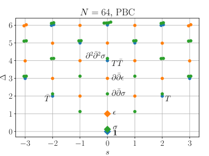
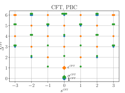
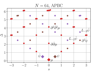
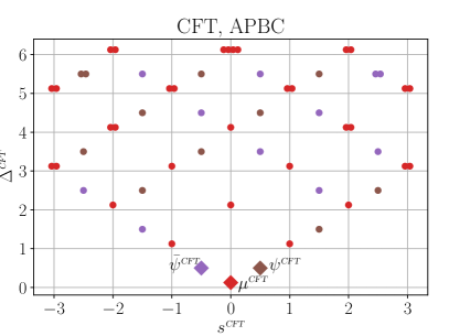
Figure 1: (Left) Low-energy spectrum of the Ising model with the PBC and the APBC at $N=64$, diagonalized using puMPS with bond dimension $D=28$. Different colors indicate different conformal towers, with diamonds labeling the primary states. We have only shown the states with conformal spins $|s|\leq 3$. (Right) The spectrum of the Ising CFT up to $\Delta^{\textsl{\tiny CFT}}\leq 6+1/8$ and $-3\leq s^{\textsl{\tiny CFT}}\leq 3$. (Note: degenerate states are plotted with a slightly shifted conformal spin to show degeneracy. For example, there are 4 descendant states of $\sigma^{\textsl{\tiny CFT}}$ at scaling dimension $6+1/8$ and conformal spin $0$.)

We can compute dimensions and conformal spins using Eqs.(29),(30),(86),(87) with different $N$, and then extrapolate the scaling dimensions to the thermodynamic limit. For example, the extrapolation for $\Delta_{\mu}$ and $\Delta_{\psi}$ is shown in Fig. (2). Table 4 shows the comparison between the numerical estimations of scaling dimensions with the exact values for all primary states and several descendant states. For completeness, we also extract the central charge with Eq. (36).

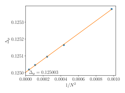
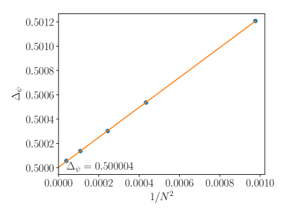
Figure 2: Extrapolation of the scaling dimensions $\Delta_{\mu}$ and $\Delta_{\psi}$ for the Ising model with $32\leq N\leq 160$.

	Exact	puMPS	error
$c$	$0.5$	0.499996	$4\times 10^{-6}$
$\Delta_{\epsilon}$	1	1.000001	$10^{-6}$
$\Delta_{\sigma}$	0.125	0.125005	$5\times 10^{-6}$
$\Delta_{\psi}$	0.5	0.500004	$4\times 10^{-6}$
$\Delta_{\bar{\psi}}$	0.5	0.500004	$4\times 10^{-6}$
$\Delta_{\mu}$	0.125	0.125003	$3\times 10^{-6}$
$\Delta_{\partial\bar{\partial}\epsilon}$	3	3.00002	$2\times 10^{-5}$
$\Delta_{T\bar{T}}$	4	4.001	$10^{-3}$
$\Delta_{\partial\bar{\partial}\sigma}$	2.125	2.12501	$10^{-5}$
$\Delta_{\partial^{2}\bar{\partial}^{2}\sigma}$	4.125	4.126	$10^{-3}$
$\Delta_{\partial^{2}\psi}$	2.5	2.499995	$5\times 10^{-6}$
$\Delta_{L_{-2}\bar{\psi}}$	2.5	2.50001	$10^{-5}$
$\Delta_{L_{-3}\bar{\psi}}$	3.5	3.50002	$2\times 10^{-5}$
$\Delta_{\partial\bar{\partial}\mu}$	2.125	2.125003	$3\times 10^{-6}$
$\Delta_{\partial^{2}\bar{\partial}^{2}\mu}$	4.125	4.1256	$6\times 10^{-4}$

Table 4: Scaling dimensions from the Ising model with $32\leq N\leq 160$.

We see that the accuracy of the scaling dimensions is better for lower-lying excited states. The errors come from two sources. First, the diagonalization with puMPS is approximate. This error can be reduced by using a larger $D$. Second, the finite-size corrections also increase with energy. This error can be reduced by simulating larger sizes $N$. In order to make a reliable extrapolation to the thermodynamic limit, we should choose sufficiently large bond dimensions $D$ such that the finite-$D$ error is much smaller than the finite-size errors. However, for a fixed bond dimension, the finite-$D$ error also increases with the energy. In the above example, the finite-$D$ error is much smaller than the finite-size error for the $|\mu\rangle$ and $|\psi\rangle$ states, as is evident from Fig. (2). However, for higher excited states such as $|T\bar{T}\rangle$, the finite-$D$ error is comparable to the finite-size error, which makes the extrapolation not as accurate.

VI.3 OPE coefficients from the Ising model

In order to extract the OPE coefficients, we first associate each lattice operator with a truncated expansion of scaling operators in the CFT, as Eqs. (31),(107) for local operators and string operators, respectively. For the purpose of finding the lattice primary operators for the Ising model, it is sufficient to limit the scaling operators in the expansion to the primary operators, i.e., $\mathbf{1}^{\textsl{\tiny CFT}},\sigma^{\textsl{\tiny CFT}},\epsilon^{\textsl{\tiny CFT}}$ in the PBC, and $\mu^{\textsl{\tiny CFT}},\psi^{\textsl{\tiny CFT}},\bar{\psi}^{\textsl{\tiny CFT}}$ in the APBC. The coefficients $a_{\alpha}$ can be obtained by minimizing the cost functions Eqs. (33),(108) for local operators and string operators, respectively. The cost function is specified by a set of low-energy eigenstates $|\psi_{\beta}\rangle$, which we choose to be the set of primary states $|\phi_{\beta}\rangle$ for simplicity. The CFT matrix elements in the cost function Eq. (33) are

$$\langle\phi^{\textsl{\tiny CFT}}_{\beta}|\phi^{\textsl{\tiny CFT},s_{\beta}}_{\alpha}|0^{\textsl{\tiny CFT}}\rangle=\left(\frac{2\pi}{L}\right)^{\Delta^{\textsl{\tiny CFT}}_{\alpha}}\delta_{\alpha\beta}.$$ (131)

The cost function Eq. (33) becomes

$$f^{\mathcal{O}}(\{a_{\alpha}\})=\sum_{\alpha}\left|\langle\phi_{\alpha}|\mathcal{O}^{s_{\alpha}}|0\rangle-\left(\frac{2\pi}{N}\right)^{\Delta^{\textsl{\tiny CFT}}_{\alpha}}a_{\alpha}\right|^{2}.$$ (132)

Its minimum is achieved by

$$a_{\alpha}=\left(\frac{2\pi}{N}\right)^{-\Delta^{\textsl{\tiny CFT}}_{\alpha}}\langle\phi_{\alpha}|\mathcal{O}^{s_{\alpha}}|0\rangle.$$ (133)

Similar expressions hold for string operators, with $\phi_{\alpha}$ APBC operators and $\mathcal{O}^{s}$ substituted with $\mathcal{S}^{s}_{\mathcal{O}}$. We will apply Eq. (133) to several lattice operators and extrapolate the $a_{\alpha}$ coefficients to the thermodynamic limit. The resulting expansions

$$\mathcal{O}\sim\sum_{\alpha}a_{\alpha}\phi^{\textsl{\tiny CFT}}_{\alpha}$$ (134)

for several operarors $\mathcal{O}$’s are shown in Table 5. We start by considering single site lattice operators $\mathcal{O}$ and add operators with larger support (two-site, etc) if they are needed to invert the expansion Eq. (134) to obtain a lattice representation of the primary fields.

For the Ising model, we have computed $a_{\alpha}$’s for local operators $\mathcal{O}_{j}=X_{j},Y_{j},Z_{j},X_{j}X_{j+1}$ and string operators $\mathcal{S}_{\mathcal{O},j}=\mathcal{S}_{I,j},\mathcal{S}_{X,j},\mathcal{S}_{Y,j}$ with $20\leq N\leq 96$. Note that the $Y$ operator does not correspond to any primary field, but to the descendant $\partial_{\tau}\sigma^{\textsl{\tiny CFT}}$ in the CFT Zou et al. (2019). We can then find lattice operators that correspond to CFT primary operators, listed in Table 5. Notice that the result is consistent with the $\mathbb{Z}_{2}$ symmetry and the Kramers-Wannier duality. For example, the lattice operator $\mathcal{O}_{\epsilon}=1.5708(XX-Z)$ is even under $\mathbb{Z}_{2}$ and odd under the duality.

Lattice	CFT
$X$	$0.80312\sigma^{\textsl{\tiny CFT}}$
$Y$	$0.0000\sigma^{\textsl{\tiny CFT}}$
$Z$	$0.63662\mathbf{1}^{\textsl{\tiny CFT}}-0.31831\epsilon^{\textsl{\tiny CFT}}$
$XX$	$0.63662\mathbf{1}^{\textsl{\tiny CFT}}+0.31831\epsilon^{\textsl{\tiny CFT}}$
$\mathcal{S}_{I}$	$0.80312\mu^{\textsl{\tiny CFT}}$
$\mathcal{S}_{X}$	$0.39894\psi^{\textsl{\tiny CFT}}+0.39894\bar{\psi}^{\textsl{\tiny CFT}}$
$\mathcal{S}_{Y}$	$-0.39894\psi^{\textsl{\tiny CFT}}+0.39894\bar{\psi}^{\textsl{\tiny CFT}}$

CFT	Lattice
$\sigma^{\textsl{\tiny CFT}}$	$1.2451X$
$\epsilon^{\textsl{\tiny CFT}}$	$1.5708XX-1.5708Z$
$\mu^{\textsl{\tiny CFT}}$	$1.2451\mathcal{S}_{X}$
$\psi^{\textsl{\tiny CFT}}$	$1.2533\mathcal{S}_{X}-1.2533\mathcal{S}_{Y}$
$\bar{\psi}^{\textsl{\tiny CFT}}$	$1.2533\mathcal{S}_{X}+1.2533\mathcal{S}_{Y}$

Table 5: Correspondence between lattice operators and CFT operators for the Ising model. (Top) Lattice operators expressed as a linear combination of a truncated set of CFT operators. (Bottom) CFT primary operators expressed as a linear combination of lattice operators by inverting the top table.

We can then use these lattice operators to compute OPE coefficients from Eqs. (95),(96). Again, an extrapolation to the thermodynamic limit is performed. For complex OPE coefficients, the real part and the imaginary part are extrapolated independently. The extrapolation of $C_{\psi\mu\sigma}$ is shown in Fig. (3) as an example.

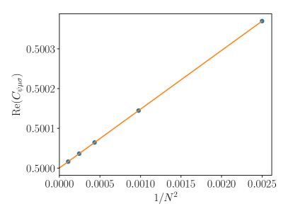
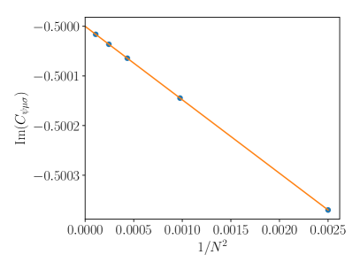
Figure 3: Extrapolation of the real and imaginary part of the OPE coefficient $C_{\psi\mu\sigma}$.

Recall that each OPE coefficient can be computed in different ways by permuting the indices, where the second index labels the lattice primary operators and the other indices label the eigenstates. We tried all possible permutation of the indices for each nontrivial OPE coefficient of the Ising model, and the results are listed in Table 6. All numerical results agree with the exact results in at least 5 digits.

OPE coefficient	Exact	Numerical
$C_{\sigma\sigma\epsilon}$	$0.5$	$0.500001$
$C_{\sigma\epsilon\sigma}$	$0.5$	$0.500000$
$C_{\mu\mu\epsilon}$	$-0.5$	$-0.500000$
$C_{\mu\epsilon\mu}$	$-0.5$	$-0.500000$
$C_{\psi\mu\sigma}$	$0.5-0.5i$	$0.500000-0.500000i$
$C_{\psi\sigma\mu}$	$0.5+0.5i$	$0.500000+0.500000i$
$C_{\mu\psi\sigma}$	$0.5+0.5i$	$0.500003+0.500003i$
$C_{\bar{\psi}\mu\sigma}$	$0.5+0.5i$	$0.500000+0.500000i$
$C_{\bar{\psi}\sigma\mu}$	$0.5-0.5i$	$0.500000-0.500000i$
$C_{\mu\bar{\psi}\sigma}$	$0.5-0.5i$	$0.500003-0.500003i$
$C_{\psi\epsilon\bar{\psi}}$	$i$	$1.00000i$
$C_{\bar{\psi}\psi\epsilon}$	$i$	$1.00001i$
$C_{\psi\bar{\psi}\epsilon}$	$-i$	$-1.00001i$

Table 6: OPE coefficients computed from the Ising model with $20\leq N\leq 96$. Numerical data are kept up to 6 digits.

We note that the expansion Eqs. (31),(107) may also involve descendant fields. This has been done in Zou et al. (2019), where the extra coefficients in the expansion are used to obtain improved lattice representations of primary fields. The finite-size corrections of OPE coefficients are reduced to $N^{-4}$. However, in this paper, we will only find lattice operators which correspond to the primary operators in the leading order. This is enough for extracting OPE coefficients.

VII The tricritical Ising model

In this section we apply our methods to a more complicated model, the tricritical Ising (TCI) model. It famously has emergent supersymmetry combined with the conformal symmmetry Friedan et al. (1985). In this section we will proceed as if we did not know about the emergent supersymmetry and extract the conformal data. In the next section we will analyze the emergent supersymmetry in more detail.

VII.1 The TCI CFT

The TCI CFT also belongs to the unitary minimal models, whose conformal data can be solved exactly. It has central charge $c^{\textsl{\tiny CFT}}=7/10$. The TCI CFT has 6 primary fields in the PBC sector, $\mathbf{1},\epsilon,\epsilon^{\prime},\epsilon^{\prime\prime},\sigma,\sigma$, and 6 primary fields in the APBC sector, $\psi,\bar{\psi},T_{F},\bar{T}_{F},\mu,\mu^{\prime}$ Lässig et al. (1991). Similar to the Ising CFT, we can also classify the above primary fields by the fermionic boundary conditions. The primary fields are summarized in Table 7. Again, operators in the NS sector can be classified with the eigenvalue under the Kramers-Wannier duality. $|\mathbf{1}\rangle,|\epsilon^{\prime}\rangle,|\bar{\psi}\rangle,|T_{F}\rangle$ are even under the duality and $|\epsilon\rangle,|\epsilon^{\prime\prime}\rangle,|\psi\rangle,|\bar{T}_{F}\rangle$ are odd Lässig et al. (1991).

$\phi^{\textsl{\tiny CFT}}_{\alpha}$	$\Delta^{\textsl{\tiny CFT}}_{\alpha}$	$s^{\textsl{\tiny CFT}}_{\alpha}$	$\mathcal{Z}_{\alpha}$	spin chain B.C.	fermion B.C.
$\mathbf{1}$	0	0	+	PBC	NS
$\epsilon$	1/5	0	+	PBC	NS
$\epsilon^{\prime}$	6/5	0	+	PBC	NS
$\epsilon^{\prime\prime}$	3	0	+	PBC	NS
$\sigma$	3/40	0	–	PBC	R
$\sigma^{\prime}$	7/8	0	–	PBC	R
$\psi$	7/10	1/2	–	APBC	NS
$\bar{\psi}$	7/10	–1/2	–	APBC	NS
$T_{F}$	3/2	3/2	–	APBC	NS
$\bar{T}_{F}$	3/2	–3/2	–	APBC	NS
$\mu$	3/40	0	+	APBC	R
$\mu^{\prime}$	7/8	0	+	APBC	R

Table 7: Virasoro primary fields of the TCI CFT.

As in the Ising CFT, we see a double degeneracy in the R sector. The degenerate states are related to each other by a supersymmetry transformation, which we will discuss in detail in the next section.

As in the Ising model, the OPE must be consistent with the $\mathbb{Z}_{2}$ symmetry and the duality. The nonzero nontrivial ones (up to permutation of indices) are

$$\mathrm{PBC-PBC-PBC}$$

$$C^{\textsl{\tiny CFT}}_{\epsilon\epsilon\epsilon^{\prime}}=c_{1},\leavevmode\nobreak\ \leavevmode\nobreak\ C^{\textsl{\tiny CFT}}_{\epsilon^{\prime}\epsilon^{\prime}\epsilon^{\prime}}=c_{1},\leavevmode\nobreak\ \leavevmode\nobreak\ C^{\textsl{\tiny CFT}}_{\epsilon\epsilon^{\prime}\epsilon^{\prime\prime}}=3/7\leavevmode\nobreak\ \leavevmode\nobreak\$$ (135)

$$C^{\textsl{\tiny CFT}}_{\sigma\sigma\epsilon}=3c_{1}/2,\leavevmode\nobreak\ \leavevmode\nobreak\ C^{\textsl{\tiny CFT}}_{\sigma\sigma\epsilon^{\prime}}=c_{1}/4,\leavevmode\nobreak\ \leavevmode\nobreak\ C^{\textsl{\tiny CFT}}_{\sigma\sigma\epsilon^{\prime\prime}}=1/56\leavevmode\nobreak\ \leavevmode\nobreak\$$ (136)

$$C^{\textsl{\tiny CFT}}_{\sigma\sigma^{\prime}\epsilon}=1/2,\leavevmode\nobreak\ \leavevmode\nobreak\ C^{\textsl{\tiny CFT}}_{\sigma\sigma^{\prime}\epsilon^{\prime}}=3/4,\leavevmode\nobreak\ \leavevmode\nobreak\ C^{\textsl{\tiny CFT}}_{\sigma^{\prime}\sigma^{\prime}\epsilon^{\prime\prime}}=7/8$$ (137)

$$\mathrm{APBC-APBC-PBC},\leavevmode\nobreak\ \leavevmode\nobreak\ \mathcal{Z}=-1,-1,+1$$

$$C^{\textsl{\tiny CFT}}_{\psi\psi\epsilon}=C^{\textsl{\tiny CFT}}_{\bar{\psi}\bar{\psi}\epsilon^{\prime}}=-c_{1}$$ (138)

$$C^{\textsl{\tiny CFT}}_{\bar{\psi}\psi\epsilon^{\prime}}=-ic_{1},\leavevmode\nobreak\ \leavevmode\nobreak\ C^{\textsl{\tiny CFT}}_{\bar{\psi}\psi\epsilon^{\prime\prime}}=3i/7$$ (139)

$$C^{\textsl{\tiny CFT}}_{\psi T_{F}\epsilon}=C^{\textsl{\tiny CFT}*}_{\bar{\psi}\bar{T}_{F}\epsilon}=-i\sqrt{3/7},\leavevmode\nobreak\ \leavevmode\nobreak\ C^{\textsl{\tiny CFT}}_{\bar{T}_{F}T_{F}\epsilon^{\prime\prime}}=-i\leavevmode\nobreak\ \leavevmode\nobreak\$$ (140)

$$C^{\textsl{\tiny CFT}}_{\bar{\psi}T_{F}\epsilon^{\prime}}=C^{\textsl{\tiny CFT}}_{\psi\bar{T}_{F}\epsilon^{\prime}}=\sqrt{3/7}$$ (141)

$$\mathrm{APBC-APBC-PBC},\leavevmode\nobreak\ \leavevmode\nobreak\ \mathcal{Z}=+1,-1,-1$$

$$C^{\textsl{\tiny CFT}}_{\mu T_{F}\sigma}=C^{\textsl{\tiny CFT}*}_{\mu\bar{T}_{F}\sigma}=\sqrt{1/56}e^{-i\pi/4}$$ (142)

$$C^{\textsl{\tiny CFT}}_{\mu^{\prime}T_{F}\sigma^{\prime}}=C^{\textsl{\tiny CFT}*}_{\mu^{\prime}\bar{T}_{F}\sigma^{\prime}}=\sqrt{7/8}e^{-3i\pi/4}$$ (143)

$$C^{\textsl{\tiny CFT}}_{\mu\psi\sigma}=C^{\textsl{\tiny CFT}*}_{\mu\bar{\psi}\sigma}=\sqrt{3/8}c_{1}e^{-i\pi/4}$$ (144)

$$C^{\textsl{\tiny CFT}}_{\mu^{\prime}\psi\sigma}=C^{\textsl{\tiny CFT}*}_{\mu^{\prime}\bar{\psi}\sigma}=\sqrt{3/8}e^{-3i\pi/4}$$ (145)

$$C^{\textsl{\tiny CFT}}_{\mu\psi\sigma^{\prime}}=C^{\textsl{\tiny CFT}*}_{\mu\bar{\psi}\sigma^{\prime}}=\sqrt{3/8}e^{-3i\pi/4}$$ (146)

$$\mathrm{APBC-APBC-PBC},\leavevmode\nobreak\ \leavevmode\nobreak\ \mathcal{Z}=+1,+1,+1$$

$$C^{\textsl{\tiny CFT}}_{\mu\mu\epsilon}=-3c_{1}/2,\leavevmode\nobreak\ C^{\textsl{\tiny CFT}}_{\mu\mu\epsilon^{\prime}}=c_{1}/4,\leavevmode\nobreak\ C^{\textsl{\tiny CFT}}_{\mu\mu\epsilon^{\prime\prime}}=-1/56\leavevmode\nobreak\ \leavevmode\nobreak\$$ (147)

$$C^{\textsl{\tiny CFT}}_{\mu^{\prime}\mu\epsilon}=-1/2,\leavevmode\nobreak\ C^{\textsl{\tiny CFT}}_{\mu^{\prime}\mu\epsilon^{\prime}}=3/4,\leavevmode\nobreak\ C^{\textsl{\tiny CFT}}_{\mu^{\prime}\mu^{\prime}\epsilon^{\prime\prime}}=-7/8,\leavevmode\nobreak\ \leavevmode\nobreak\ \leavevmode\nobreak\ \leavevmode\nobreak\$$ (148)

where

$$c_{1}=\frac{2}{3}\sqrt{\frac{\Gamma(4/5)\Gamma^{3}(2/5)}{\Gamma(1/5)\Gamma^{3}(3/5)}}\approx 0.61030.$$ (149)

The OPE coefficients of the PBC primary operators are taken from Mossa and Mussardo (2008). We note that the OPE coefficient $C^{\textsl{\tiny CFT}}_{\sigma^{\prime}\sigma^{\prime}\epsilon^{\prime\prime}}$ was written in Lässig et al. (1991) as $7c_{1}/8$, instead of $7/8$ in Eq. (137). Our numerical result below agrees with Mossa and Mussardo (2008). OPE coefficients involving APBC operators are generally complex. Their phases depend on the convention of the normalization of scaling operators. Here we have chosen the convention such that they match the lattice calculations below.

VII.2 Scaling dimensions, conformal spins and central charge from the TCI model

We use puMPS with bond dimension $20\leq D\leq 44$ to diagonalize the low-energy spectrum of the TCI model with both boundary conditions for $20\leq N\leq 80$. Similar to the Ising model, we plot the low-energy eigenstates up to scaling dimension $\Delta^{\textsl{\tiny CFT}}\leq 3.2$ for the PBC and $\Delta^{\textsl{\tiny CFT}}\leq 2.7$ for the APBC. The result is shown in Fig. (4). We also see that all eigenstates corresponding to the CFT scaling operators in this range are captured by the puMPS ansatz.

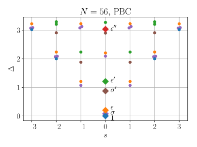
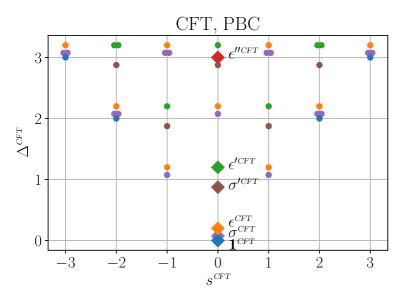
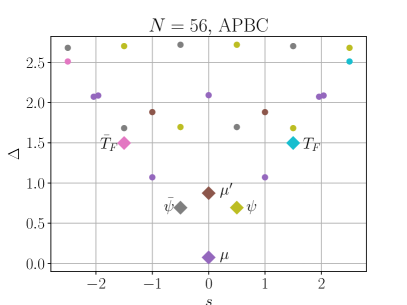
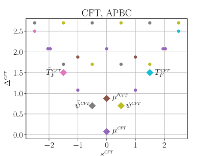
Figure 4: (Left) Low-energy spectrum of the TCI model with PBC and APBC at $N=56$, diagonalized using puMPS with bond dimension $D=36$. Different colors indicate different conformal towers, with diamonds labeling the primary states. The exceptions are that the $\sigma(\sigma^{\prime})$ and $\mu(\mu^{\prime})$ towers are plotted with the same color. (Right) The spectrum of the TCI CFT up to $\Delta^{\textsl{\tiny CFT}}\leq 3.2$ for PBC and $\Delta^{\textsl{\tiny CFT}}\leq 2.7$ for APBC.

Again, scaling dimensions and the central charge can be extracted with an extrapolation to the thermodynamic limit. The result is shown in Table 8. For simplicity we only show the scaling dimensions of the primary states. We see the error occurs after 3 significant digits, which roughly agrees with the accuracy of the tricritical point $\lambda^{*}$ in Eq. (51).

	Exact	puMPS	error
$c$	$0.7$	0.6987	$1.3\times 10^{-3}$
$\Delta_{\epsilon}$	0.2	0.2002	$2\times 10^{-4}$
$\Delta_{\epsilon^{\prime}}$	1.2	1.203	$3\times 10^{-3}$
$\Delta_{\epsilon^{\prime\prime}}$	3	3.006	$6.0\times 10^{-3}$
$\Delta_{\sigma}$	0.075	0.07493	$7\times 10^{-5}$
$\Delta_{\sigma^{\prime}}$	0.875	0.8748	$2\times 10^{-4}$
$\Delta_{\psi}$	0.7	0.6979	$2.1\times 10^{-3}$
$\Delta_{\bar{\psi}}$	0.7	0.6979	$2.1\times 10^{-3}$
$\Delta_{T_{F}}$	1.5	1.500	$1\times 10^{-4}$
$\Delta_{\bar{T}_{F}}$	1.5	1.500	$1\times 10^{-4}$
$\Delta_{\mu}$	0.075	0.07493	$7\times 10^{-5}$
$\Delta_{\mu^{\prime}}$	0.875	0.8748	$2\times 10^{-4}$

Table 8: Scaling dimensions from the TCI model. All numerical values are extrapolated using $40\leq N\leq 80$, except $\Delta_{\epsilon^{\prime\prime}}$ where we use $20\leq N\leq 56$. All numerical values are kept to 4 significant digits.

VII.3 OPE coefficients from the TCI model

Following the general prescription in Section II and IV, we first need to construct lattice operators corresponding to CFT primary fields variationally. Here we choose to compute lattice representations of $\epsilon,\epsilon^{\prime},\sigma,\sigma^{\prime},\mu,\mu^{\prime},\psi,\bar{\psi},T_{F},\bar{T}_{F}$. These operators correspond to $\Delta^{\textsl{\tiny CFT}}_{\alpha}\leq 1.2$ in the PBC sector and $\Delta^{\textsl{\tiny CFT}}_{\alpha}\leq 1.5$ in the APBC sector. Notice that we will not construct the lattice operator for $\epsilon^{\prime\prime}$ with $\Delta^{\textsl{\tiny CFT}}_{\epsilon^{\prime\prime}}=3$ because it is numerically difficult. The reason is that it requires a linear combination of many lattice operators with fine-tuned coefficients such that all contributions with lower scaling dimensions vanish. With an extrapolation of the finite-size $a_{\alpha}$’s, we obtain the results listed in Table 9.

Lattice	CFT
$X$	$0.7808\sigma^{\textsl{\tiny CFT}}-0.1866\sigma^{\prime\textsl{\tiny CFT}}$
$XZ+ZX$	$0.3551\sigma^{\textsl{\tiny CFT}}-0.9060\sigma^{\prime\textsl{\tiny CFT}}$
$Z$	$0.5821\mathbf{1}^{\textsl{\tiny CFT}}-0.4753\epsilon^{\textsl{\tiny CFT}}-0.1760\epsilon^{\prime\textsl{\tiny CFT}}$
$XX$	$0.5821\mathbf{1}^{\textsl{\tiny CFT}}+0.4753\epsilon^{\textsl{\tiny CFT}}-0.1760\epsilon^{\prime\textsl{\tiny CFT}}$
$\mathcal{S}_{I}$	$0.7808\mu^{\textsl{\tiny CFT}}-0.1866\mu^{\prime\textsl{\tiny CFT}}$
$\mathcal{S}_{XX}-\mathcal{S}_{YY}$	$0.3551\mu^{\textsl{\tiny CFT}}-0.9060\mu^{\prime\textsl{\tiny CFT}}$
$\mathcal{S}_{X}$	$0.4042(\psi^{\textsl{\tiny CFT}}+\bar{\psi}^{\textsl{\tiny CFT}})+0.2462(T^{\textsl{\tiny CFT}}_{F}+\bar{T}^{\textsl{\tiny CFT}}_{F})$
$\mathcal{S}_{Y}$	$-0.4042(\psi^{\textsl{\tiny CFT}}-\bar{\psi}^{\textsl{\tiny CFT}})+0.2462(T^{\textsl{\tiny CFT}}_{F}-\bar{T}^{\textsl{\tiny CFT}}_{F})$
$\mathcal{S}_{IX}$	$0.4695(\psi^{\textsl{\tiny CFT}}+\bar{\psi}^{\textsl{\tiny CFT}})+0.0829(T^{\textsl{\tiny CFT}}_{F}+\bar{T}^{\textsl{\tiny CFT}}_{F})$
$\mathcal{S}_{YZ}$	$-0.4695(\psi^{\textsl{\tiny CFT}}-\bar{\psi}^{\textsl{\tiny CFT}})+0.0829(T^{\textsl{\tiny CFT}}_{F}-\bar{T}^{\textsl{\tiny CFT}}_{F})$

CFT	Lattice
$\sigma^{\textsl{\tiny CFT}}$	$1.413X-0.2910(XZ+ZX)$
$\sigma^{\prime\textsl{\tiny CFT}}$	$0.5539X-1.218(XZ+ZX)$
$\epsilon^{\textsl{\tiny CFT}}$	$1.052XX-1.052Z$
$\epsilon^{\prime\textsl{\tiny CFT}}$	$3.307I-2.841XX-2.841Z$
$\mu^{\textsl{\tiny CFT}}$	$1.413\mathcal{S}_{I}-0.2910(\mathcal{S}_{XX}-\mathcal{S}_{YY})$
$\mu^{\prime\textsl{\tiny CFT}}$	$0.5539\mathcal{S}_{I}-1.218(\mathcal{S}_{XX}-\mathcal{S}_{YY})$
$\psi^{\textsl{\tiny CFT}}$	$-0.5072(\mathcal{S}_{X}-\mathcal{S}_{Y})+1.506(\mathcal{S}_{IX}-\mathcal{S}_{YZ})$
$\bar{\psi}^{\textsl{\tiny CFT}}$	$-0.5072(\mathcal{S}_{X}+\mathcal{S}_{Y})+1.506(\mathcal{S}_{IX}+\mathcal{S}_{YZ})$
$T^{\textsl{\tiny CFT}}_{F}$	$2.860(\mathcal{S}_{X}+\mathcal{S}_{Y})-2.462(\mathcal{S}_{IX}+\mathcal{S}_{YZ})$
$\bar{T}^{\textsl{\tiny CFT}}_{F}$	$2.860(\mathcal{S}_{X}-\mathcal{S}_{Y})-2.462(\mathcal{S}_{IX}-\mathcal{S}_{YZ})$

Table 9: Correspondence between lattice operators and CFT operators for the O’Brien-Fendley model. (Top) Correspondence between some lattice operators and a linear combination of CFT primary operators. (Bottom) Lattice operators that correspond to CFT primary operators.

OPE coefficient	Exact	Numerical
$C_{\sigma\sigma\epsilon}$	$0.9155$	$0.9154$
$C_{\sigma\sigma\epsilon^{\prime}}$	$0.1526$	$0.1531$
$C_{\sigma\sigma\epsilon^{\prime\prime}}$	$0.0179$	$0.0177$
$C_{\sigma^{\prime}\sigma\epsilon}$	$0.5$	$0.5007$
$C_{\sigma^{\prime}\sigma\epsilon^{\prime}}$	$0.75$	$0.752$
$C_{\sigma^{\prime}\sigma^{\prime}\epsilon^{\prime\prime}}$	$0.875$	$0.869$
$C_{\epsilon\epsilon\epsilon^{\prime}}$	$0.610$	$0.608$
$C_{\epsilon^{\prime}\epsilon\epsilon^{\prime\prime}}$	$0.429$	$0.437$
$C_{\epsilon^{\prime}\epsilon^{\prime}\epsilon^{\prime}}$	$0.61$	$0.58$

OPE coefficient	Exact	Numerical
$C_{\psi T_{F}\epsilon}$	$-0.655i$	$-0.662i$
$C_{\bar{\psi}T_{F}\epsilon^{\prime}}$	$0.655$	$0.664$
$C_{\bar{T}_{F}T_{F}\epsilon^{\prime\prime}}$	$-i$	$-0.03-1.02i$
$C_{\bar{\psi}\bar{T}_{F}\epsilon}$	$0.655i$	$0.662i$
$C_{\psi\bar{T}_{F}\epsilon^{\prime}}$	$0.655$	$0.664$
$C_{\psi\psi\epsilon^{\prime}}$	$-0.610$	$-0.613$
$C_{\bar{\psi}\bar{\psi}\epsilon^{\prime}}$	$-0.610$	$-0.613$
$C_{\bar{\psi}\psi\epsilon}$	$0.610i$	$0.612i$
$C_{\bar{\psi}\psi\epsilon^{\prime\prime}}$	$0.43i$	$0.01+0.41i$

Table 10: OPE coefficients of the TCI CFT computed from the TCI model. The organization of the table follows the exact results listed before. All numerical results are kept to the last significant digits, and the exact results are shown with the same number of significant digit. All OPE coefficients involving $\epsilon^{\prime\prime}$ are extrapolated with data from $20\leq N\leq 56$, while those not involving $\epsilon^{\prime\prime}$ are extrapolated with data from $32\leq N\leq 72$.

OPE coefficient	Exact	Numerical
$C_{\mu T_{F}\sigma}$	$0.094-0.094i$	$0.097-0.097i$
$C_{\mu\bar{T}_{F}\sigma}$	$0.094+0.094i$	$0.097+0.097i$
$C_{\mu^{\prime}T_{F}\sigma^{\prime}}$	$-0.661+0.661i$	$-0.669+0.669i$
$C_{\mu^{\prime}\bar{T}_{F}\sigma^{\prime}}$	$-0.661-0.661i$	$-0.669-0.669i$
$C_{\mu\psi\sigma}$	$0.265-0.265i$	$0.264-0.264i$
$C_{\mu\psi\sigma^{\prime}}$	$-0.433+0.433i$	$-0.434+0.434i$
$C_{\mu^{\prime}\psi\sigma}$	$-0.433+0.433i$	$-0.434+0.434i$
$C_{\mu\bar{\psi}\sigma}$	$0.264+0.264i$	$0.264+0.264i$
$C_{\mu^{\prime}\bar{\psi}\sigma}$	$-0.433-0.433i$	$-0.434-0.434i$
$C_{\mu^{\prime}\bar{\psi}\sigma}$	$-0.433-0.433i$	$-0.434-0.434i$

OPE coefficient	Exact	Numerical
$C_{\mu\mu\epsilon}$	$-0.9154$	$-0.9153$
$C_{\mu\mu\epsilon^{\prime}}$	$0.1526$	$0.1532$
$C_{\mu\mu\epsilon^{\prime\prime}}$	$-0.0179$	$-0.0172$
$C_{\mu^{\prime}\mu\epsilon}$	$-0.5$	$-0.5008$
$C_{\mu^{\prime}\mu\epsilon^{\prime}}$	$0.75$	$0.752$
$C_{\mu^{\prime}\mu^{\prime}\epsilon^{\prime\prime}}$	$-0.875$	$-0.86$

Table 11: OPE coefficients of the TCI CFT computed from the TCI model, continued.

We can then work out all OPE coefficients $C_{\alpha\beta\gamma}$ where $\phi_{\beta}\neq\epsilon^{\prime\prime}$ with Eqs. (95),(96). For those OPE coefficients that are related by permuting indices, we will only show one particular order of indices for simplicity, e.g., we will compute $C_{\sigma\sigma\epsilon}$ but not $C_{\sigma\epsilon\sigma}$. With indices appropriately permuted, only the computation of $C_{\epsilon^{\prime\prime}\epsilon^{\prime\prime}\epsilon^{\prime\prime}}$ requires a lattice operator for $\epsilon^{\prime\prime}$, but we know $C^{\textsl{\tiny CFT}}_{\epsilon^{\prime\prime}\epsilon^{\prime\prime}\epsilon^{\prime\prime}}$ vanishes because $\epsilon^{\prime\prime}$ is odd under Kramers-Wannier duality. Therefore in this case we can still extract a complete set of nonvanishing OPE coefficients, see Tables 10, 11.

VIII Emergence of superconformal symmetry in the tricritical Ising model

In this section we study the emergent superconformal symmetry in the TCI model. We first review the $\mathcal{N}=1$ superconformal algebra. We then show how to find the lattice operators that correspond to supervirasoro generators. We verify the action of the supervirasoro generators on low energy subspaces of the TCI model with both PBC and APBC. Some matrix elements are checked quantitatively with analytical results. In particular, a formula analogous to Eq. (36) for the central charge is proposed and checked numerically.

VIII.1 $\mathcal{N}=1$ supersymmetry and the TCI model

The $\mathcal{N}=1$ supersymmetry for $1+1$ dimensional quantum field theories is defined with two supercharges $Q^{\textsl{\tiny QFT}}$ and $\bar{Q}^{\textsl{\tiny QFT}}$ which satisfy

$$Q^{\textsl{\tiny QFT}\dagger} = Q^{\textsl{\tiny QFT}}$$ (150)

$$\bar{Q}^{\textsl{\tiny QFT}\dagger} = \bar{Q}^{\textsl{\tiny QFT}}$$ (151)

$$\leavevmode\nobreak\ [Q^{\textsl{\tiny QFT}},\bar{Q}^{\textsl{\tiny QFT}}] = 0$$ (152)

$$H^{\textsl{\tiny QFT}} = (Q^{\textsl{\tiny QFT}})^{2}+(\bar{Q}^{\textsl{\tiny QFT}})^{2}.$$ (153)

The supercharges are fermionic operators. They map bosonic excitations into fermionic excitations and vice versa.

Each supercharge is associated with a supersymmetry current, $T^{\textsl{\tiny QFT}}_{F},\bar{T}^{\textsl{\tiny QFT}}_{F}$, which are the density of the supercharges,

$$Q^{\textsl{\tiny QFT}}=\int dx\,T^{\textsl{\tiny QFT}}_{F}(x),\leavevmode\nobreak\ \leavevmode\nobreak\ \bar{Q}^{\textsl{\tiny QFT}}=\int dx\,\bar{T}^{\textsl{\tiny QFT}}_{F}(x).$$ (154)

For a lattice model which flows into a supersymmetric quantum field theory, such as the TCI model Eq. (51), the lattice version of Eqs. (152),(153) may not be exact. As pointed out by O’brien and Fendley O’Brien and Fendley (2018), the TCI Hamiltonian with density Eq. (51) can be expressed as

$$H_{\textsl{\tiny TCI}}=Q^{2}+\bar{Q}^{2}+E_{0},$$ (155)

where $E_{0}$ is an energy shift, and

$$Q =\sum_{j}T_{F,j}$$ (156)

$$T_{F,j} \propto(\gamma_{2j-1}+\gamma_{2j})+2i\lambda^{*}(\gamma_{2j-2}+\gamma_{2j+1})\gamma_{2j-1}\gamma_{2j}$$ (157)

$$\bar{Q} =\sum_{j}\bar{T}_{F,j}$$ (158)

$$\bar{T}_{F,j} \propto(\gamma_{2j-1}-\gamma_{2j})+2i\lambda^{*}(\gamma_{2j+1}-\gamma_{2j-2})\gamma_{2j-1}\gamma_{2j},$$ (159)

where $2\lambda^{*}\approx 0.856$. In terms of string operators, they are

$$T_{F}\propto(\mathcal{S}_{X}+\mathcal{S}_{Y})-2\lambda^{*}(\mathcal{S}_{YZ}+\mathcal{S}_{IX}),$$ (160)

$$\bar{T}_{F}\propto(\mathcal{S}_{X}-\mathcal{S}_{Y})+2\lambda^{*}(\mathcal{S}_{YZ}-\mathcal{S}_{IX}).$$ (161)

It is simple to check that $Q$ and $\bar{Q}$ are Hermitian but $[Q,\bar{Q}]\neq 0$. Therefore, supersymmetry is not exact on the lattice. However, it has been shown numerically O’Brien and Fendley (2018) that, under the RG flow, not only $Q$ and $\bar{Q}$ flow to the supercharges, but also $T_{F}$ and $\bar{T}_{F}$ flow to the supersymmetry currents. In the previous section, we have variationally found $T_{F,j}$ and $\bar{T}_{F,j}$ (Table 9) without exploiting Eq. (155),

$$T_{F}=2.86[(\mathcal{S}_{X}+\mathcal{S}_{Y})-0.861(\mathcal{S}_{YZ}+\mathcal{S}_{IX})],$$ (162)

$$\bar{T}_{F}=2.86[(\mathcal{S}_{X}-\mathcal{S}_{Y})+0.861(\mathcal{S}_{YZ}-\mathcal{S}_{IX})].$$ (163)

They agree quantitatively with Eqs. (160),(161) up to normalization, with the error in the third digit.

We also note that in O’Brien and Fendley (2018) the lattice operators corresponding to $\psi^{\textsl{\tiny CFT}}$ and $\bar{\psi}^{\textsl{\tiny CFT}}$ were also proposed,

$$\psi\propto(\mathcal{S}_{X}-\mathcal{S}_{Y})-2\lambda^{*}(\mathcal{S}_{YZ}-\mathcal{S}_{IX}),$$ (164)

$$\bar{\psi}\propto(\mathcal{S}_{X}+\mathcal{S}_{Y})+2\lambda^{*}(\mathcal{S}_{YZ}+\mathcal{S}_{IX}).$$ (165)

In this paper we obtain a very different coefficient between the two terms (see Table 9). However, the two results do not contradict each other. They both correspond to $\psi^{\textsl{\tiny CFT}}(\bar{\psi}^{\textsl{\tiny CFT}})$ as the leading contribution, but our result also eliminates the contribution from $T^{\textsl{\tiny CFT}}_{F},\bar{T}^{\textsl{\tiny CFT}}_{F}$. In this sense, we provide an improved lattice operator corresponding to $\psi^{\textsl{\tiny CFT}}$ (as well as $\bar{\psi}^{\textsl{\tiny CFT}}$).

VIII.2 The superconformal algebra

If conformal symmetry is enhanced by the supersymmetry, the resulting quantum field theory is a superconformal field theory (SCFT). In a SCFT, the supercurrent $T^{\textsl{\tiny CFT}}_{F}(\bar{T}^{\textsl{\tiny CFT}}_{F})$ are Virasoro primary fields with conformal dimensions $(3/2,0)$ and $(0,3/2)$, respectively. Expanding $T^{\textsl{\tiny CFT}}_{F}$ in Fourier modes gives supervirasoro generators

$$G^{\textsl{\tiny CFT}}_{n}=\left(\frac{2\pi}{L}\right)^{-1/2}\int_{0}^{L}dx\,T^{\textsl{\tiny CFT}}_{F}(x)e^{inx2\pi/L}.$$ (166)

Together with $L^{\textsl{\tiny CFT}}_{n}$, they satisfy the superconformal algebra

$$[L^{\textsl{\tiny CFT}}_{n},L^{\textsl{\tiny CFT}}_{m}] =(n-m)L^{\textsl{\tiny CFT}}_{n+m}+\frac{c^{\textsl{\tiny CFT}}}{12}n(n^{2}-1)\delta_{n+m,0}$$ (167)

$$\leavevmode\nobreak\ [L^{\textsl{\tiny CFT}}_{n},G^{\textsl{\tiny CFT}}_{m}] =\left(\frac{1}{2}n-m\right)G^{\textsl{\tiny CFT}}_{n+m}$$ (168)

$$\leavevmode\nobreak\ \{G^{\textsl{\tiny CFT}}_{n},G^{\textsl{\tiny CFT}}_{m}\} =2L^{\textsl{\tiny CFT}}_{n+m}+\frac{c^{\textsl{\tiny CFT}}}{3}\left(n^{2}-\frac{1}{4}\right)\delta_{n+m,0},$$ (169)

where the first identity is the Virasoro algebra, the second identity follows from the fact that $T^{\textsl{\tiny CFT}}_{F}$ is a primary field with conformal dimensions $(3/2,0)$, and the third identity is the crucial feature of a supersymmetric theory that the anticommutator of two supersymmetry generators yields the generator of a spacetime transformation. Analogous to the Virasoro algebra, there is a copy of the same superconformal algebra for the anti-holomorphic generators $\bar{L}^{\textsl{\tiny CFT}}_{n},\bar{G}^{\textsl{\tiny CFT}}_{m}$. Since $T^{\textsl{\tiny CFT}}_{F}$ is a fermionic field, it follows that $m\in\mathbb{Z}+1/2$ for the NS boundary condition, and $m\in\mathbb{Z}$ for the R boundary condition. The corresponding superconformal algebras are called the NS algebra and the R algebra, respectively.

Let us analyze the action of the supervirasoro generators in more detail. First, let $n=0$ in Eq. (168). We obtain

$$[L^{\textsl{\tiny CFT}}_{0},G^{\textsl{\tiny CFT}}_{m}]=-mG^{\textsl{\tiny CFT}}_{m},$$ (170)

which means that $G^{\textsl{\tiny CFT}}_{m}$ changes the holomorphic dimension by $-m$. Therefore, $G^{\textsl{\tiny CFT}}_{m}$ with $m<0$ is a raising operator, whereas with $m>0$ a lowering operator. A superconformal primary state $|\Phi^{\textsl{\tiny CFT}}_{\alpha}\rangle$ is defined by

$$L^{\textsl{\tiny CFT}}_{n}|\Phi^{\textsl{\tiny CFT}}_{\alpha}\rangle=0,\leavevmode\nobreak\ \leavevmode\nobreak\ G^{\textsl{\tiny CFT}}_{m}|\Phi^{\textsl{\tiny CFT}}_{\alpha}\rangle=0,\leavevmode\nobreak\ (n,m>0)$$ (171)

$$\bar{L}^{\textsl{\tiny CFT}}_{n}|\Phi^{\textsl{\tiny CFT}}_{\alpha}\rangle=0,\leavevmode\nobreak\ \leavevmode\nobreak\ \bar{G}^{\textsl{\tiny CFT}}_{m}|\Phi^{\textsl{\tiny CFT}}_{\alpha}\rangle=0,\leavevmode\nobreak\ (n,m>0).$$ (172)

By virtue of Eqs. (167),(168), the above equalities hold for all $n>0,m>0$ if they hold for $n=1,2$ and $m=1/2,3/2$ for the NS algebra (or $m=1$ for the R algebra).

In the $R$ algebra, $G^{\textsl{\tiny CFT}}_{0}$ needs more attention. First, Eq. (169) implies

$$(G^{\textsl{\tiny CFT}}_{0})^{2}=L^{\textsl{\tiny CFT}}_{0}-\frac{c^{\textsl{\tiny CFT}}}{24}.$$ (173)

Then, the Hamiltonian can be written as

$$H^{\textsl{\tiny CFT}}=\frac{2\pi}{L}((G^{\textsl{\tiny CFT}}_{0})^{2}+(\bar{G}^{\textsl{\tiny CFT}}_{0})^{2}),$$ (174)

which follows from Eq. (13). We see that $G^{\textsl{\tiny CFT}}_{0}$ and $\bar{G}^{\textsl{\tiny CFT}}_{0}$ are proportional to supercharges, in accordance with Eqs. (153),(166). Second, $G^{\textsl{\tiny CFT}}_{0}$ commutes with $L^{\textsl{\tiny CFT}}_{0}$. This means that $G_{0}|\Phi^{\textsl{\tiny CFT}}_{\alpha}\rangle$, if non-vanishing, has the same conformal dimensions as $|\Phi^{\textsl{\tiny CFT}}_{\alpha}\rangle$. Eq. (173) implies that $G_{0}|\Phi^{\textsl{\tiny CFT}}_{\alpha}\rangle$ is nonvanishing if

$$h^{\textsl{\tiny CFT}}_{\alpha}\neq\frac{c^{\textsl{\tiny CFT}}}{24}.$$ (175)

If this is true for some supervirasoro primary state in the R sector, the supervirasoro primary state is at least double degenerate. As a result, all descendant states will also be at least double degenerate. In this case the supersymmetry is said to be spontaneously broken Friedan et al. (1985). We have seen that indeed there is a double degeneracy for each state in the R sector of the TCI model, one in the PBC of the spin chain and the other in the APBC of the spin chain.

VIII.3 Supervirasoro primary states in the TCI CFT

As noted in the previous section, there are 12 Virasoro primary states in the TCI CFT, where 8 of them are in the NS sector and 4 of them are in the R sector. In the R sector, all Virasoro primary states are also supervirasoro primary states. $\sigma^{\textsl{\tiny CFT}}(\sigma^{\prime\textsl{\tiny CFT}})$ is the superpartner of $\mu^{\textsl{\tiny CFT}}(\mu^{\prime\textsl{\tiny CFT}})$. They are related by the supercharge $Q^{\textsl{\tiny CFT}}\propto G^{\textsl{\tiny CFT}}_{0}$,

$$G^{\textsl{\tiny CFT}}_{0}|\sigma^{\textsl{\tiny CFT}}\rangle = a_{\sigma}|\mu^{\textsl{\tiny CFT}}\rangle$$ (176)

$$G^{\textsl{\tiny CFT}}_{0}|\sigma^{\prime\textsl{\tiny CFT}}\rangle = a_{\sigma^{\prime}}|\mu^{\prime\textsl{\tiny CFT}}\rangle,$$ (177)

where

$$a_{\alpha}=\sqrt{h^{\textsl{\tiny CFT}}_{\alpha}-\frac{c^{\textsl{\tiny CFT}}}{24}},$$ (178)

by virtue of Eq. (173), where $h^{\textsl{\tiny CFT}}_{\sigma}=3/80$, $h^{\textsl{\tiny CFT}}_{\sigma^{\prime}}=7/16$, $c^{\textsl{\tiny CFT}}=7/10$.

In the NS sector, only $\mathbf{1}^{\textsl{\tiny CFT}}$ and $\epsilon^{\textsl{\tiny CFT}}$ are superconformal primary states. The rest of virasoro primary states are connected to the supervirasoro primary states by the $G^{\textsl{\tiny CFT}}_{m}$, shown in Fig.(5). The matrix elements are

$$\langle\psi^{\textsl{\tiny CFT}}|G^{\textsl{\tiny CFT}}_{-1/2}|\epsilon^{\textsl{\tiny CFT}}\rangle = \langle\bar{\psi}^{\textsl{\tiny CFT}}|\bar{G}^{\textsl{\tiny CFT}}_{-1/2}|\epsilon^{\textsl{\tiny CFT}}\rangle=a_{\epsilon}$$ (179)

$$\langle\epsilon^{\prime\textsl{\tiny CFT}}|G^{\textsl{\tiny CFT}}_{-1/2}|\bar{\psi}^{\textsl{\tiny CFT}}\rangle = \langle\epsilon^{\prime\textsl{\tiny CFT}}|\bar{G}^{\textsl{\tiny CFT}}_{-1/2}|\psi^{\textsl{\tiny CFT}}\rangle=a_{\epsilon}$$ (180)

$$\langle T^{\textsl{\tiny CFT}}_{F}|G^{\textsl{\tiny CFT}}_{-3/2}|0^{\textsl{\tiny CFT}}\rangle = \langle\bar{T}^{\textsl{\tiny CFT}}_{F}|\bar{G}^{\textsl{\tiny CFT}}_{-3/2}|0^{\textsl{\tiny CFT}}\rangle=a_{\mathbf{1}}$$ (181)

$$\langle\epsilon^{\prime\prime\textsl{\tiny CFT}}|G^{\textsl{\tiny CFT}}_{-3/2}|\bar{T}^{\textsl{\tiny CFT}}_{F}\rangle = \langle\epsilon^{\prime\prime\textsl{\tiny CFT}}|\bar{G}^{\textsl{\tiny CFT}}_{-3/2}|T^{\textsl{\tiny CFT}}_{F}\rangle=a_{\mathbf{1}},$$ (182)

where $a_{\epsilon}=\sqrt{2h^{\textsl{\tiny CFT}}_{\epsilon}}=1/\sqrt{5}$ and $a_{\mathbf{1}}=\sqrt{2c^{\textsl{\tiny CFT}}/3}=\sqrt{7/15}$. They can be derived from the superconformal algebra (see Appendix). These matrix elements indicate that $|\psi^{\textsl{\tiny CFT}}\rangle,|\bar{\psi}^{\textsl{\tiny CFT}}\rangle,|\epsilon^{\prime\textsl{\tiny CFT}}\rangle$ are supervirasoro descendants of $|\epsilon^{\textsl{\tiny CFT}}\rangle$, and $|T^{\textsl{\tiny CFT}}_{F}\rangle,|\bar{T}^{\textsl{\tiny CFT}}_{F}\rangle,|\epsilon^{\prime\prime\textsl{\tiny CFT}}\rangle$ are supervirasoro descendants of $|\mathbf{1}^{\textsl{\tiny CFT}}\rangle$.

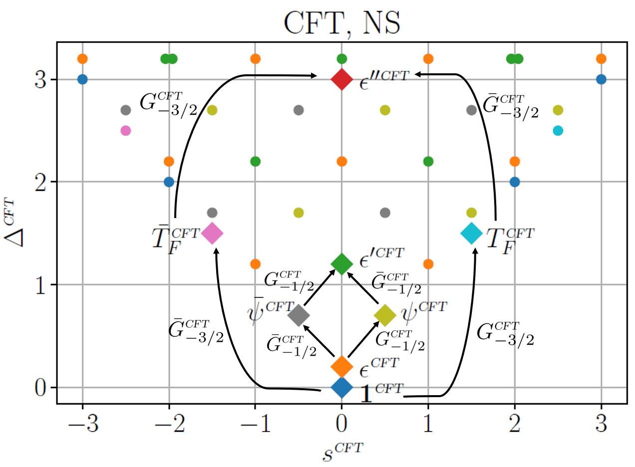
Figure 5: Spectrum of the TCI CFT in the NS sector. Primary states are labelled as diamonds. Arrows indicate that the primary states are related by the supervirasoro generators $G^{\textsl{\tiny CFT}}_{m}$.

VIII.4 Lattice supervirasoro generators

In the CFT, the supervirasoro generators are Fourier modes of the fermionic stress tensors, Eq. (166). Therefore, we expect that on the lattice Fourier modes of the string operator $T_{F}$ also realize the supervirasoro operators at low energies. Recall the definition Eq. (98),

$$G_{n}=\eta\sum_{j=1}^{N}\tilde{\mathcal{T}}^{j-1}T_{F,1}\mathcal{T}^{\dagger j-1}e^{inj2\pi/N},$$ (183)

where $\mathcal{T}$ and $\tilde{\mathcal{T}}$ are translation operators for the Hamiltonian with PBC and APBC, respectively, and $\eta$ is a normalization factor. The equation above applies to both the NS sector ($n\in 1/2+\mathbb{Z}$) and the R sector ($n\in\mathbb{Z}$). To fix the normalization factor $\eta$, we require that

$$\langle T_{F}|G_{1/2}|T\rangle=\sqrt{3}.$$ (184)

This comes from the CFT identity (derivation in Appendix)

$$\langle T^{\textsl{\tiny CFT}}_{F}|G^{\textsl{\tiny CFT}}_{1/2}|T^{\textsl{\tiny CFT}}\rangle=\sqrt{3}.$$ (185)

Note that both $|T^{\textsl{\tiny CFT}}\rangle$ and $|T^{\textsl{\tiny CFT}}_{F}\rangle$ necessarily exist in a SCFT, such that the normalization condition Eq. (184) is universally applicable.

Below we compare the matrix elements of $G_{n}$ with the CFT matrix elements Eqs. (176)-(182). In particular, Eq. (181) provides a way of verifying that central charge in Eqs. (167) and (169) are the same,

$$c^{\prime}=\frac{3}{2}|\langle T_{F}|G_{-3/2}|0\rangle|^{2},$$ (186)

which equals the central charge $c^{\textsl{\tiny CFT}}$ in the thermodynamic limit. This equation can be viewed as the ”superpartner” of Eq. (36). The result is shown in Fig. (6), where we also plot the result of Eq. (36) for comparison. We obtain $c^{\prime}=0.701$ and $c=0.699$, with the errors on the same order. The other matrix elements in the NS sector are plotted in Fig.(7). We see that all matrix elements shown in the figure approximately converge to the nonzero CFT values Eqs. (179), (180), and (182) in the thermodynamic limit. Similarly, we can compute the matrix elements of $\bar{G}_{n}$, which are the Fourier modes of $\bar{T}_{F}$, and see that they agree with the CFT values in the thermodynamic limit. Therefore, we have verified in the TCI model that $|\psi\rangle,|\bar{\psi}\rangle,|\epsilon^{\prime}\rangle$ are supervirasoro descendants of $|\epsilon\rangle$, and $|T_{F}\rangle,|\bar{T}_{F}\rangle,|\epsilon^{\prime\prime}\rangle$ are supervirasoro descendants of $|\mathbf{1}\rangle$. The only supervirasoro primaries in the NS sector, are therefore, $|\mathbf{1}\rangle$ and $|\epsilon\rangle$

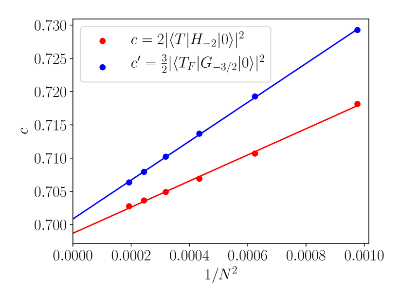
Figure 6: The central charge from Eqs. (36),(181).

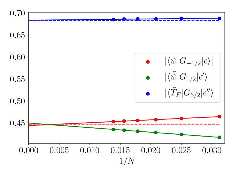
Figure 7: Matrix elements of $G_{n}$ in the NS sector of the TCI model. The dashed lines represent the corresponding CFT matrix element Eqs. (179),(180),(182). The CFT matrix elements Eqs. (179),(180) have the same modulus, so we only show one of them in the figure.

In the R sector, we can similarly compute the matrix elements of $G_{n}$ ($n\in\mathbb{Z}$). An important example is $G_{0}$ that relates superpartners, as in Eqs. (176) and (177). The matrix elements can be computed on the lattice, shown in Fig. (8). We also see that the numerical results agree with the CFT matrix elements.

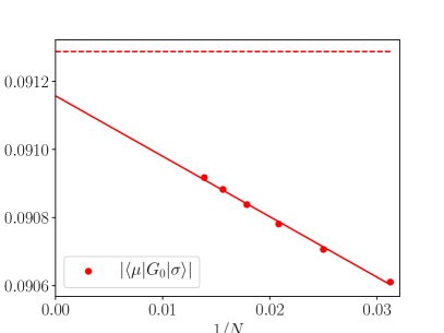
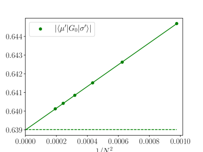
Figure 8: Matrix elements of $G_{n}$ in the R sector of the TCI model. The dashed lines represent the corresponding CFT matrix elements in Eqs. (176),(177).

To conclude, we have proposed the lattice supervirasoro generators $G_{n}$ as Fourier modes of the lattice string operator $T_{F}$, where the latter is found variationally. We have examined the action of $G_{n}$ in both NS and R sectors and seen that it agrees with the supervirasoro algebra. The whole construction only relies on the low-energy spectrum of the critical quantum spin chain. Therefore we expect that the above lattice construction of $G_{n}$ gives a generic method to identify supervirasoro primaries and superconformal towers.

IX Conclusion

In this paper, we have generalized the method Zou et al. (2018, 2019) of extracting conformal data from a critical quantum spin chains from PBC to APBC.

Starting with the lattice Hamiltonian density, we first build the Hamiltonians $H^{\textsl{\tiny PBC}}$ and $H^{\textsl{\tiny APBC}}$ with PBC and APBC. We then diagonalize the low-energy eigenstates with both boundary conditions and various sizes $N$. To go beyond exact diagonalization, a tensor network method based on periodic uniform matrix product states can be used. The scaling dimensions $\Delta_{\alpha}$ and conformal spins $s_{\alpha}$ of scaling operators can be extracted from the energies $E_{\alpha}$ and momenta $P_{\alpha}$ of the eigenstates with both boundary conditions. Fourier modes $H_{n}$ of the Hamiltonian density with respect to the translation operator $\mathcal{T}$ ($\tilde{\mathcal{T}}$) of the (A)PBC Hamiltonian act as a linear combination of Virasoro generators on the low-energy subspace with (A)PBC. They allow us to identify each eigenstate with a CFT scaling operator. In particular, primary states and their conformal towers are identified. The central charge can be extracted with the matrix elements of $H_{-2}$.

We have shown that local operators correspond to PBC operators in the CFT, and that string operators correspond to APBC operators in the CFT. Given a lattice operator, we can associate it with a truncated linear combination of CFT scaling operators, whose coefficients are determined by minimizing a cost function. The lattice operators that correspond to CFT primary fields can be obtained by inverting the truncated linear expansion. OPE coeffcients can then be extracted from the matrix elements of the Fourier modes of the local or string operators that correspond to CFT primary fields. In the case of emergent superconformal symmetry, the fermionic stress tensor states $|T_{F}\rangle,|\bar{T}_{F}\rangle$ are always present in the low-energy spectrum of $H^{\textsl{\tiny APBC}}$. The lattice supervirasoro generators $G_{n},\bar{G}_{n}$ can be constructed as Fourier modes of the string operators that correspond to $T_{F},\bar{T}_{F}$. They can be used to identify supervirasoro primary states and supervirasoro conformal towers. The matrix element of $G_{-3/2}$ gives another estimation of the central charge, which converges to the central charge of the SCFT in the thermodynamic limit.

As an illustration of the general method, we have extracted complete conformal data of the Ising CFT and TCI CFT from the Ising spin chain and the TCI spin chain. We have correctly identified all primary states and their conformal towers. Scaling dimensions, conformal spins, the central charges and all OPE coefficients are obtained with high accuracy. For the TCI model, we have verified the action of the lattice supervirasoro generators on the low-energy eigenstates and showed that they agree with the expectation from the superconformal algebra. We stress that the only input of our method is the critical lattice Hamiltonian. It is interesting to apply our method to the cases where the underlying CFT has not been completely solved.

Apart from a complete set of conformal data, generators of extended symmetries (if any) can also be constructed on the lattice. In this paper we have investigated the superconformal symmetry, but other extended symmetry can be treated in the same way, such as the Kac-Moody algebra Wang et al. (2019).

Our method can be generalized to other twisted boundary conditions that preserve emergent conformal symmetry. For an on-site symmetry defect, the generalization is straightforward. It is still an open question how to deal with more general conformal defects with our method. We would like to point out that for some topological conformal defects other methods such as tensor network renormalization Hauru et al. (2016) and entanglement renormalization Evenbly et al. (2010) are available.

Acknowlegments — We thank Cenke Xu, Andreas Ludwig, Zhenghan Wang, Ashley Milsted and Martin Ganahl for useful discussions and valuable comments. The authors acknowledge support from the Simons Foundation (Many Electron Collaboration) and Compute Canada. G. Vidal is a CIFAR fellow in the Quantum Information Science Program. Research at Perimeter Institute is supported by the Government of Canada through the Department of Innovation, Science and Economic Development Canada and by the Province of Ontario through the Ministry of Research, Innovation and Science. X is formerly known as Google[x] and is part of the Alphabet family of companies, which includes Google, Verily, Waymo, and others (www.x.company).

Appendix A puMPS algorithm for APBC

In this section we detail the puMPS algorithm for eigenstates with APBC, and how to compute matrix elements of local or string operators involving them. It is a straightforward generalization of the algorithm for eigenstates with PBC, which has been described in detail in Zou et al. (2018).

A.1 Computing low-energy eigenstates

Recall the ansatz for APBC eigenstates with momentum $p$,

$$|\Phi^{\textsl{\tiny APBC}}_{p}(B;A)\rangle=\sum_{j=1}^{N}e^{-ipj}\tilde{\mathcal{T}}^{j}\sum_{\vec{s}=1}^{d}\mathrm{Tr}(B^{s_{1}}A^{s_{2}}\cdots A^{s_{N}})|\vec{s}\rangle,$$ (187)

where $A$ is the puMPS tensor for the PBC ground state, satisfying

$$\sum_{s^{\prime}}\mathcal{Z}_{ss^{\prime}}A^{s^{\prime}}=U_{B}(\mathcal{Z})A^{s}U^{\dagger}_{B}(\mathcal{Z}),$$ (188)

and $B=B^{s}_{ab}$ contains the variational parameters to be computed.

In Zou et al. (2018), a reparametrization of the excitation ansatz has been shown useful for PBC eigenstates. Here we will use the same trick for APBC eigenstates. The trick consists of two steps. First, there is a gauge choice of the ground state puMPS tensor $A^{s}=A^{s}_{C}\lambda^{-1}$, where $A^{s}_{C}$ is a $D\times D$ matrix and $\lambda$ is $D\times D$ diagonal matrix, such that $A^{s}_{L}\equiv A^{s}=A^{s}_{C}\lambda^{-1}$ satisfies the left canonical condition and $A^{s}_{R}\equiv\lambda^{-1}A^{s}_{C}$ satisfies the right canonical condition. Second, we will reparameterize $B^{s}=B^{s}_{C}\lambda^{-1}$. The new parameterization consists of a $d\times D\times D$ tensor $B_{C}$ as variational parameters,

$$\,\,\,\,\,\,\,\,|\Phi^{\textsl{\tiny APBC}}_{p}(B_{C};A_{L})\rangle$$

$$=\sum_{j=1}^{N}e^{-ipj}\tilde{\mathcal{T}}^{j}\sum_{\vec{s}=1}^{d}\mathrm{Tr}((B^{s_{1}}_{C}\lambda^{-1})A^{s_{2}}_{L}\cdots A^{s_{N}}_{L})|\vec{s}\rangle.$$ (189)

Below we use $\mu=(s,a,b)$ to denote the combined index of the physical and bond indices.

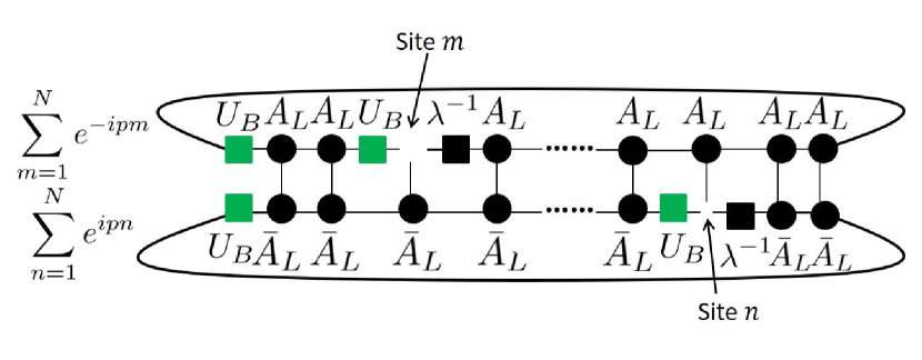
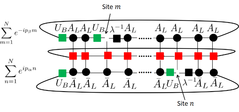
Figure 9: (Top) The tensor network for $N^{\textsl{\tiny APBC}}_{\mu\nu}(p)$ in Eq. (192). The green tensor $U_{B}\equiv U_{B}(\mathcal{Z})$ in Eq. (116). (Bottom) The tensor network for $H^{\textsl{\tiny APBC}}_{\mu\nu}(p)$ in Eq. (193) if the red tensors form a matrix product operator (MPO) for the Hamiltonian $H$ and $p_{\alpha}=p_{\beta}=p$. It also represents $O_{\mu\nu}(p_{\alpha},p_{\beta})$ in Eq. (A.2) if the red tensors form a MPO for $\tilde{O}^{s}$.

Our approximation of the eigenstates of the Hamiltonian are obtained as the saddle point of the energy functional,

$$E_{p}(B_{C},\bar{B}_{C};A_{L},\bar{A}_{L})=\frac{\langle\Phi^{\textsl{\tiny APBC}}_{p}(\bar{B}_{C};\bar{A}_{L})|H|\Phi^{\textsl{\tiny APBC}}_{p}(B_{C};A_{L})\rangle}{\langle\Phi^{\textsl{\tiny APBC}}_{p}(\bar{B}_{C};\bar{A}_{L})|\Phi^{\textsl{\tiny APBC}}_{p}(B_{C};A_{L})\rangle}.$$ (190)

The saddle point condition translates into a generalized eigenvalue equation for $B^{\mu}_{C}$,

$$H^{\textsl{\tiny APBC}}_{\mu\nu}(p)B^{\nu}_{C}=EN^{\textsl{\tiny APBC}}_{\mu\nu}(p)B^{\nu}_{C},$$ (191)

where

$$N^{\textsl{\tiny APBC}}_{\mu\nu}(p) = \left\langle\frac{\partial}{\partial\bar{B}^{\mu}_{C}}\Phi^{\textsl{\tiny APBC}}_{p}(\bar{B}_{C};\bar{A}_{L})\right.\left|\frac{\partial}{\partial B^{\nu}_{C}}\Phi^{\textsl{\tiny APBC}}_{p}(B_{C};A_{L})\right\rangle\leavevmode\nobreak\ \leavevmode\nobreak\ \leavevmode\nobreak\ \leavevmode\nobreak\ \leavevmode\nobreak\ \leavevmode\nobreak\$$ (192)

$$H^{\textsl{\tiny APBC}}_{\mu\nu}(p) = \left\langle\frac{\partial}{\partial\bar{B}^{\mu}_{C}}\Phi^{\textsl{\tiny APBC}}_{p}(\bar{B}_{C};\bar{A}_{L})\right|H\left|\frac{\partial}{\partial B^{\nu}_{C}}\Phi^{\textsl{\tiny APBC}}_{p}(B_{C};A_{L})\right\rangle.\leavevmode\nobreak\ \leavevmode\nobreak\ \leavevmode\nobreak\ \leavevmode\nobreak\ \leavevmode\nobreak\ \leavevmode\nobreak\$$ (193)

They are depicted as tensor networks in Fig. 9. Note that the action of $\tilde{\mathcal{T}}=\mathcal{Z}_{1}\mathcal{T}$ can be viewed as first acting with the ordinary translation operator and then acting with $\mathcal{Z}_{1}$, where the latter can be lifted to the bond indices by using Eq. (188). Contracting the tensor networks has the same leading cost $\mathcal{O}(ND^{6})$ as the PBC case. The only difference from the case of PBC is the $U_{B}$ tensors appearing in the contraction. The periodic MPO for the Hamiltonian with PBC can be further decomposed into a MPO for the Hamiltonian with OBC and a local boundary term. This further lowers the cost compared to directly contracting the network with the periodic MPO.

The generalized eigenvalue equation Eq. (191) can be translated into an ordinary eigenvalue problem by multiplying the pseudoinverse of $N^{\textsl{\tiny APBC}}_{\mu\nu}$ on both sides,

$$\tilde{N}^{\textsl{\tiny APBC},\rho\mu}(p)H^{\textsl{\tiny APBC}}_{\mu\nu}(p)B^{\nu}_{C}=EB^{\rho}_{C},$$ (194)

where $\tilde{N}^{\textsl{\tiny APBC}}(p)$ is the pseudoinverse of $N^{\textsl{\tiny APBC}}(p)$. Then Eq. (194) can be solved in each momentum sector with a sparse eigenvalue solver such as the Arnoldi method.

A.2 Computing matrix elements of local operators

Matrix elements of a Fourier mode of a local operator in the low-energy basis of $H^{\textsl{\tiny APBC}}$ are bilinear functions of the $B$ tensors in Eq. (187),

$$\,\,\,\,\,\,\,\,\langle\Phi^{\textsl{\tiny APBC}}_{p_{\alpha}}(\bar{B}_{C,\alpha};\bar{A}_{L})|\tilde{\mathcal{O}}^{s}|\Phi^{\textsl{\tiny APBC}}_{p_{\beta}}(B_{C,\beta};A_{L})\rangle$$

$$=\bar{B}^{\mu}_{C,\alpha}\mathcal{O}_{\mu\nu}(p_{\alpha},p_{\beta})B^{\nu}_{C,\beta}.$$ (195)

This expression is nonzero only if momentum is conserved,

$$p_{\alpha}=\frac{2\pi}{N}s+p_{\beta}.$$ (196)

The matrix $\mathcal{O}_{\mu\nu}(p_{\alpha},p_{\beta})$ is plotted at the bottom of Fig. 9. The contraction also costs $\mathcal{O}(ND^{6})$.

A.3 Computing matrix elements of string operators

Matrix elements of a Fourier mode of a string operator are also bilinear functions of the $B$ tensors.

$$\,\,\,\,\,\,\,\,\,\langle\Phi^{\textsl{\tiny APBC}}_{p_{\alpha}}(\bar{B}_{C,\alpha};\bar{A}_{L})|\mathcal{S}^{s}_{\mathcal{O}}|\Phi^{\textsl{\tiny PBC}}_{p_{\beta}}(B_{C,\beta};A_{L})\rangle$$

$$=\bar{B}^{\mu}_{C,\alpha}\mathcal{S}_{\mathcal{O},\mu\nu}(p_{\alpha},p_{\beta})B^{\nu}_{C,\beta}.$$ (197)

Note that the ket is now a PBC low-energy eigenstate, and the bra is a APBC low-energy eigenstate. The conservation of momentum is necessary for the matrix element to be nonzero,

$$p_{\alpha}=\frac{2\pi}{N}s+p_{\beta}.$$ (198)

Although string operators are nonlocal, they can be represented efficiently with a MPO. This means that $\mathcal{S}_{\mathcal{O},\mu\nu}(p_{\alpha},p_{\beta})$ can be represented as the same network as the bottom network of Fig. 9, except that the $U_{B}$ tensors in the upper layer are removed. Therefore the computation of $\mathcal{S}_{\mathcal{O},\mu\nu}(p_{\alpha},p_{\beta})$ has the same leading cost $\mathcal{O}(ND^{6})$ as the computation of $\mathcal{O}_{\mu\nu}(p_{\alpha},p_{\beta})$.

If $\mathcal{O}$ is a one-site operator, then $\mathcal{S}^{s}_{\mathcal{O}}$ can be encoded in a MPO with bond dimension $2$,

$$\begin{bmatrix}1&0\end{bmatrix}\prod_{j=1}^{N}\begin{bmatrix}Z_{j}&\mathcal{O}_{j}e^{-isj}\\ 0&I_{j}\end{bmatrix}\begin{bmatrix}0\\ 1\end{bmatrix}.$$ (199)

If $\mathcal{O}$ is supported on $n$ sites, then an additional boundary term appears. In this case, $\mathcal{S}^{s}_{\mathcal{O}}$ can be decomposed into a MPO with bond dimension $n+1$ with open boundary conditions and a boundary term. For example, consider

$$\mathcal{S}^{s}_{YZ}=\sum_{j=1}^{N-1}e^{-isj2\pi/N}\left(\prod_{l=1}^{j-1}Z_{l}\right)Y_{j}Z_{j+1}+\mathcal{B}^{s}_{YZ},$$ (200)

where the sum can be encoded in a MPO with open boundary conditions and bond dimenson $3$, and the boundary term is

$$\mathcal{B}^{s}_{YZ}=e^{-is2\pi}I_{1}\left(\prod_{l=2}^{N-1}Z_{l}\right)Y_{N}.$$ (201)

If we act with $\mathcal{B}^{s}_{YZ}$ on a PBC eigenstate with parity $\mathcal{Z}_{\alpha}$, then the action can be further simplified,

$$\mathcal{B}^{s}_{YZ}|\psi^{\textsl{\tiny PBC}}_{\alpha}\rangle=e^{-is2\pi}(iX_{N}Z_{1})\mathcal{Z}_{\alpha}|\psi^{\textsl{\tiny PBC}}_{\alpha}\rangle.$$ (202)

We see that the net effect of the boundary term of $\mathcal{S}^{s}_{\mathcal{O}}$ acting on a PBC eigenstate is equivalent to a local boundary term. Again we decompose $\mathcal{S}^{s}_{\mathcal{O}}$ into a MPO with OBC and a local boundary term. This lowers the computational cost compared to directly contracting the tensor network with a periodic MPO.

Appendix B Fourier mode of multi-site operators and string operators

Recall that the Fourier mode of a local operator $\mathcal{O}$ is defined by

$$\mathcal{O}^{s}=\frac{1}{N}\sum_{j=1}^{N}e^{-isx_{j}2\pi/N}\mathcal{O}_{j},$$ (203)

where $x_{j}$ is the position of the operator $\mathcal{O}_{j}$ with support starting at site $j$. For a one-site operator, $x_{j}=j$. (In the main text we have use $j$ instead of $x_{j}$ for simplicity of notation.) However, this choice of $x_{j}$ is ambiguous for a multi-site operator, since it can be anywhere inside the support. It has been shown Zou et al. (2019) that the corresponding CFT operator $\mathcal{O}^{\textsl{\tiny CFT}}$ can change by a total spatial derivative if the choice of $x_{j}$ is changed. Similarly, a string operator

$$\mathcal{S}_{\mathcal{O},j}=\left(\prod_{l=1}^{j-1}Z_{l}\right)\mathcal{O}_{j}.$$ (204)

can be assigned some position $x_{j}$. The choice of $x_{j}$ affects the corresponding CFT operator up to a total spatial derivative.

However, in the main text we have only considered the coefficients $a_{\alpha}$ of primary operators $\phi^{\textsl{\tiny CFT}}_{\alpha}$ in the truncated expansion of $\mathcal{O}^{\textsl{\tiny CFT}}$. The $a_{\alpha}$’s in the thermodynamic limit do not depend on the choice of $x_{j}$ since primary operators are not total spatial derivatives. Nevertheless, there is a preferred choice Zou et al. (2019) of $x_{j}$ which makes the finite-size scaling of the $a_{\alpha}$’s better, because they forbid some of the derivative descendants in the expansion of $\mathcal{O}^{\textsl{\tiny CFT}}$ by symmetry. In this appendix, we list our choices of $x_{j}$ for both local and string operators that have appeared in the main text.

For a local operator $\mathcal{O}_{j}$, if it is $\mathbb{Z}_{2}$ odd and its support ranges from site $j$ to $j+n$, then we follow the ”middle point rule”, i.e., $x_{j}=j+n/2$. If the operator is $\mathbb{Z}_{2}$ even, we first rewrite it as a local product of Majorana operators. The Majorana operator $\gamma_{j^{\prime}}$ is assigned position $x_{j^{\prime}}=j^{\prime}/2+1/4$. If the product of Majorana operators has support from $\gamma_{j^{\prime}}$ to $\gamma_{j^{\prime}+n^{\prime}}$, then we follow the ”middle point rule” $x_{j}=x_{j^{\prime}}+n^{\prime}/4=(2j^{\prime}+n^{\prime}+1)/4$. (Notice that two adjacent Majorana modes have a distance $1/2$ rather than $1$.)

If a string operator is $\mathbb{Z}_{2}$ odd, then it can be rewritten as a local product of Majorana operators. We can then use the ”middle point rule”. If the string operator is $\mathbb{Z}_{2}$ even, then we first use a Jordan-Wigner transformation to obtain a $\mathbb{Z}_{2}$ odd local operator, then the position of the string operator is assigned to the position of the local operator minus $1/2$. In summary, we list the result of $x_{j}$ for the operators that have appeared in the main text in Table 12.

$\mathcal{O}_{j}$	$x_{j}$	$\mathcal{S}_{\mathcal{O},j}$	$x_{j}$
$X_{j}$	$j$	$\mathcal{S}_{I,j}$	$j-\frac{1}{2}$
$Y_{j}$	$j$	$\mathcal{S}_{X,j}$	$j-\frac{1}{4}$
$Z_{j}$	$j$	$\mathcal{S}_{Y,j}$	$j+\frac{1}{4}$
$X_{j}X_{j+1}$	$j+\frac{1}{2}$	$\mathcal{S}_{YZ,j}$	$j+\frac{3}{4}$
$X_{j}Z_{j+1}$	$j+\frac{1}{2}$	$\mathcal{S}_{IX,j}$	$j+\frac{1}{4}$
$Z_{j}X_{j+1}$	$j+\frac{1}{2}$	$\mathcal{S}_{XX,j}$	$j$
$X_{j}X_{j+1}Z_{j+2}$	$j+\frac{5}{4}$	$\mathcal{S}_{YY,j}$	$j+1$
$Z_{j}X_{j+1}X_{j+2}$	$j+\frac{3}{4}$

Table 12: Position assignment $x_{j}$ of local operators $\mathcal{O}_{j}$ and string operators $\mathcal{S}_{\mathcal{O},j}$.

Appendix C CFT matrix elements with the supervirasoro algebra

In this appendix we derive the CFT matrix elements for the TCI CFT used in the main text. We will omit the CFT superscript because we will only compute quantities in the CFT. First, the central charge Eq. (186) can be obtained by

$$\,\,\,\,\,\,\,\,|\langle T_{F}|G_{-3/2}|0\rangle|^{2}$$ (205)

$$=\langle 0|G_{3/2}G_{-3/2}|0\rangle$$ (206)

$$=\langle 0|\{G_{3/2},G_{-3/2}\}|0\rangle$$ (207)

$$=\frac{2c}{3},$$ (208)

where in the second line we use the fact that $G_{-3/2}$ acting on the ground state only gives the $|T_{F}\rangle$ state, in the third line we use the fact that $G_{3/2}$ annihilates the ground state, and in the last line we use the supervirasoro algebra and that $L_{0}$ annihilates the ground state. We can choose the phase of $G_{n}$ such that

$$\langle T_{F}|G_{-3/2}|0\rangle=\sqrt{\frac{2c}{3}}.$$ (209)

Similar calculation can be performed on other matrix elements. For example, in the NS sector we can compute

$$\,\,\,\,\,\,\,\,|\langle\psi|G_{-1/2}|\epsilon\rangle|^{2}$$ (210)

$$=\langle\epsilon|G_{1/2}G_{-1/2}|\epsilon\rangle$$ (211)

$$=\langle\epsilon|\{G_{1/2},G_{-1/2}\}|\epsilon\rangle$$ (212)

$$=\langle\epsilon|2L_{0}|\epsilon\rangle$$ (213)

$$=\Delta_{\epsilon}+s_{\epsilon}$$ (214)

$$=0.2$$ (215)

and

$$\,\,\,\,\,\,\,\,|\langle\epsilon^{\prime}|\bar{G}_{-1/2}|\psi\rangle|^{2}$$ (216)

$$=\langle\psi|\bar{G}_{1/2}\bar{G}_{-1/2}|\psi\rangle$$ (217)

$$=\langle\psi|2\bar{L}_{0}|\psi\rangle$$ (218)

$$=\Delta_{\psi}-s_{\psi}$$ (219)

$$=0.2.$$ (220)

In the R sector we can compute

$$\,\,\,\,\,\,\,\,|\langle\mu|G_{0}|\sigma\rangle|^{2}$$ (221)

$$=\langle\sigma|G^{2}_{0}|\sigma\rangle$$ (222)

$$=\langle\sigma|L_{0}-\frac{c}{24}|\sigma\rangle$$ (223)

$$=h_{\sigma}-\frac{c}{24}.$$ (224)

Similarly $|\langle\mu^{\prime}|G_{0}|\sigma^{\prime}\rangle|^{2}$ can be computed.

Finally, let us verify the normalization condition of $G_{n}$, Eq. (185).

$$\,\,\,\,\,\,\,\,\langle T_{F}|G_{1/2}|T\rangle$$ (225)

$$=\sqrt{\frac{3}{2c}}\langle 0|G_{3/2}G_{1/2}|T\rangle$$ (226)

$$=\sqrt{\frac{3}{2c}}\langle 0|2L_{2}|T\rangle$$ (227)

$$=\sqrt{\frac{3}{2c}}2\sqrt{\frac{c}{2}}$$ (228)

$$=\sqrt{3},$$ (229)

where in the second line we use Eq. (209), in the third line we use the supervirasoro algebra and the fact that $G_{3/2}$ annihilates $|T\rangle$, and in the fourth line we use Eq. (36).

References

- Wilson and Kogut (1974) K. G. Wilson and J. Kogut, Phys. Rep. 12, 75 (1974).
- Belavin et al. (1984) A. A. Belavin, A. M. Polyakov, and A. B. Zamolodchikov, Nucl. Phys. B 241, 333 (1984).
- Friedan et al. (1984) D. Friedan, Z. Qiu, and S. Shenker, Phys. Rev. Lett. 52, 1575 (1984).
- Ginsparg (1988) P. Ginsparg, lecture notes (1988), arXiv:hep-th/9108028 .
- Henkel (1999) M. Henkel, Conformal Invariance and Critical Phenomena (Springer, New York, 1999).
- Di Francesco et al. (2012) P. Di Francesco, P. Mathieu, and D. Senechal, Conformal Field Theory (Springer, New York, 2012).
- Cardy (1984a) J. L. Cardy, J. Phys. A: Math. Gen. 17, L385 (1984a).
- Blöte et al. (1986) H. W. J. Blöte, J. L. Cardy, and M. P. Nightingale, Phys. Rev. Lett. 56, 742 (1986).
- Affleck (1986) I. Affleck, Phys. Rev. Lett. 56, 746 (1986).
- Cardy (1986a) J. L. Cardy, Nucl. Phys. B 270, 186 (1986a).
- Koo and Saleur (1994) W. M. Koo and H. Saleur, Nucl. Phys. B 426, 459 (1994), arXiv:hep-th/9312156 .
- Milsted and Vidal (2017) A. Milsted and G. Vidal, Phys. Rev. B 96, 245105 (2017), arXiv:1706.01436 .
- Zou et al. (2019) Y. Zou, A. Milsted, and G. Vidal, (2019), arXiv:1901.06439 [cond-mat.str-el] .
- Zou et al. (2018) Y. Zou, A. Milsted, and G. Vidal, Phys. Rev. Lett. 121, 230402 (2018), arXiv:1710.05397 .
- Cardy (1984b) J. L. Cardy, Journal of Physics A: Mathematical and General 17, L961 (1984b).
- Cardy (1989) J. L. Cardy, Nuclear Physics B 324, 581 (1989).
- Friedan et al. (1985) D. Friedan, Z. Qiu, and S. Shenker, Physics Letters B 151, 37 (1985).
- O’Brien and Fendley (2018) E. O’Brien and P. Fendley, Phys. Rev. Lett. 120, 206403 (2018), arXiv:1712.06662 .
- Cardy (1986b) J. L. Cardy, J. Phys. A: Math. Gen. 19, L1093 (1986b).
- Note (1) For a multi-site operator , there is an ambiguity with the definition of the Fourier mode Eq. (32\@@italiccorr), addressed in Ref.Zou et al. (2019) and further illustrated in appendix.
- Read and Saleur (2007) N. Read and H. Saleur, Nucl. Phys. B 777, 316 (2007), arXiv:hep-th/0701117 .
- Dubail et al. (2010) J. Dubail, J. L. Jacobsen, and H. Saleur, Nucl. Phys. B 834, 399 (2010), arXiv:1001.1151 .
- Vasseur et al. (2012) R. Vasseur, A. M. Gainutdinov, J. L. Jacobsen, and H. Saleur, Phys. Rev. Lett. 108, 161602 (2012), arXiv:1110.1327 .
- Gainutdinov et al. (2013) A. M. Gainutdinov, J. L. Jacobsen, N. Read, H. Saleur, and R. Vasseur, J. Phys. A: Math. Theor. 46, 494012 (2013), arXiv:1303.2082 .
- Gainutdinov and Vasseur (2013) A. M. Gainutdinov and R. Vasseur, Nucl. Phys. B 868, 223 (2013), arXiv:1203.6289 .
- Bondesan et al. (2015) R. Bondesan, J. Dubail, A. Faribault, and Y. Ikhlef, J. Phys. A: Math. Theor. 48, 065205 (2015), arXiv:1409.8590 .
- White (1992) S. R. White, Phys. Rev. Lett. 69, 2863 (1992).
- Fannes et al. (1992) M. Fannes, B. Nachtergaele, and R. F. Werner, Commun. Math. Phys. 144, 443 (1992).
- Rommer and Östlund (1997) S. Rommer and S. Östlund, Phys. Rev. B 55, 2164 (1997).
- Vidal (2004) G. Vidal, Phys. Rev. Lett. 93, 040502 (2004).
- Vidal (2007) G. Vidal, Phys. Rev. Lett. 99, 220405 (2007), arXiv:cond-mat/0512165 .
- Degli et al. (2004) C. Degli, E. Boschi, and F. Ortolani, Eur. Phys. J. B 41, 503 (2004).
- Tagliacozzo et al. (2008) L. Tagliacozzo, T. R. de Oliveira, S. Iblisdir, and J. I. Latorre, Phys. Rev. B 78, 024410 (2008), arXiv:0712.1976 .
- Xavier (2010) J. C. Xavier, Phys. Rev. B 81, 224404 (2010), arXiv:1002.0531 .
- Stojevic et al. (2015) V. Stojevic, J. Haegeman, I. P. McCulloch, L. Tagliacozzo, and F. Verstraete, Phys. Rev. B 91, 035120 (2015), arXiv:1401.7654 .
- Schollwöck (2011) U. Schollwöck, Annals of Physics 326, 96 (2011).
- Pirvu et al. (2011) B. Pirvu, F. Verstraete, and G. Vidal, Phys. Rev. B 83, 125104 (2011).
- Pirvu et al. (2012) B. Pirvu, J. Haegeman, and F. Verstraete, Phys. Rev. B 85, 035130 (2012), arXiv:1103.2735 .
- Henkel (1987) M. Henkel, Journal of Physics A: Mathematical and General 20, 995 (1987).
- Burkhardt and Guim (1985) T. W. Burkhardt and I. Guim, Journal of Physics A: Mathematical and General 18, L33 (1985).
- Aasen et al. (2016) D. Aasen, R. S. K. Mong, and P. Fendley, Journal of Physics A: Mathematical and Theoretical 49, 354001 (2016).
- Hauru et al. (2016) M. Hauru, G. Evenbly, W. W. Ho, D. Gaiotto, and G. Vidal, Phys. Rev. B 94, 115125 (2016), arXiv:1512.03846 .
- Ramond (1971) P. Ramond, Phys. Rev. D 3, 2415 (1971).
- Neveu and Schwarz (1971) A. Neveu and J. H. Schwarz, Physics Letters B 34, 517 (1971).
- Jordan and Wigner (1928) P. Jordan and E. Wigner, Zeitschrift fur Physik 47, 631 (1928).
- Rahmani et al. (2015a) A. Rahmani, X. Zhu, M. Franz, and I. Affleck, Phys. Rev. B 92, 235123 (2015a), arXiv:1505.03966 .
- Rahmani et al. (2015b) A. Rahmani, X. Zhu, M. Franz, and I. Affleck, Phys. Rev. Lett. 115, 166401 (2015b), arXiv:1504.05192 .
- Zauner-Stauber et al. (2018) V. Zauner-Stauber, L. Vanderstraeten, J. Haegeman, I. P. McCulloch, and F. Verstraete, Phys. Rev. B 97, 235155 (2018), arXiv:1802.07197 .
- Verstraete and Cirac (2006) F. Verstraete and J. I. Cirac, Phys. Rev. B 73, 094423 (2006), arXiv:cond-mat/0505140 .
- Singh et al. (2010) S. Singh, R. N. C. Pfeifer, and G. Vidal, Phys. Rev. A 82, 050301 (2010), arXiv:0907.2994 .
- Singh et al. (2011) S. Singh, R. N. C. Pfeifer, and G. Vidal, Phys. Rev. B 83, 115125 (2011), arXiv:1008.4774 .
- Singh and Vidal (2013) S. Singh and G. Vidal, Phys. Rev. B 88, 115147 (2013), arXiv:1307.1522 .
- Francesco et al. (1987) P. D. Francesco, H. Saleur, and J. Zuber, Nuclear Physics B 290, 527 (1987).
- Boyanovsky (1989) D. Boyanovsky, Phys. Rev. B 39, 6744 (1989).
- Hsieh et al. (2016) T. H. Hsieh, G. B. Halász, and T. Grover, Phys. Rev. Lett. 117, 166802 (2016), arXiv:1604.08591 .
- Lässig et al. (1991) M. Lässig, G. Mussardo, and J. L. Cardy, Nucl. Phys. B 348, 591 (1991).
- Mossa and Mussardo (2008) A. Mossa and G. Mussardo, Journal of Statistical Mechanics: Theory and Experiment 2008, P03010 (2008).
- Wang et al. (2019) R. Wang, Y. Zou, and G. Vidal, Upcoming (2019).
- Evenbly et al. (2010) G. Evenbly, P. Corboz, and G. Vidal, Phys. Rev. B 82, 132411 (2010), arXiv:0912.2166 .