Deep Generative Quantile-Copula Models for Probabilistic Forecasting

Abstract

We introduce a new category of multivariate conditional generative models and demonstrate its performance and versatility in probabilistic time series forecasting and simulation. Specifically, the output of quantile regression networks is expanded from a set of fixed quantiles to the whole Quantile Function by a univariate mapping from a latent uniform distribution to the target distribution. Then the multivariate case is solved by learning such quantile functions for each dimension’s marginal distribution, followed by estimating a conditional Copula to associate these latent uniform random variables. The quantile functions and copula, together defining the joint predictive distribution, can be parameterized by a single implicit generative Deep Neural Network.

1 Introduction

We start by describing implicit generative models of which the proposed model is an instance, then motivations in the frontier of the challenges in probabilistic time series forecasting and simulation.

Implicit Generative Models Consider learning a conditional joint distribution $p(\mathbf{y}|\mathbf{x})$ from data observations, where $\mathbf{y}$ is a $d$-dimensional target random vector and $\mathbf{x}$ is a feature vector, through an implicit generative model (IGM) $\mathbf{y}=g(\mathbf{x},\mathbf{z})$. Here $\mathbf{z}$ is some latent random noise used to capture all the underlying randomness in $\mathbf{y}$ given $\mathbf{x}$, through a deterministic generator function $g(\cdot)$, parameterized by a deep neural net. The unsupervised version, without covariates $\mathbf{x}$, is the more popular formulation in literature with state-of-the-art solutions in image and text generation. Generative adversarial networks (GAN, Goodfellow et al, 2014) map $\hat{\mathbf{y}}=g(\mathbf{z})$ by training $g(\cdot)$ to fool a classifier telling real $\mathbf{y}$ from the generated $\hat{\mathbf{y}}$. GANs suffer from stability issues in training and complex constraints of the critic function in its variants (e.g. WGAN, Arjovsky et al, 2017). The learning principle of GAN-style IGMs is comparison by samples (Mohamed and Lakshminarayanan, 2016), basically comparing the empirical distribution between an observations set and the generated samples set, e.g. adversarial/f-divergence/moment-matching losses. This approach falls short in conditional generative modeling: the specific context $\mathbf{x}$ of an observation usually appears only once in the dataset, thus it is difficult to do sub-population comparison. This issue naturally leads to the use of proper scoring rules (Gneiting and Raftery, 2007) which compare a single observation against a predictive distribution. Flow-based generative models (Dinh et al, 2014/2016) learn by maximizing log-likelihood, the most common scoring rule. Flow-based models restrict the mapping $\mathbf{y}=g(\mathbf{z})$ to be invertible and the Jacobian determinant $|\mathrm{d}g^{-1}(\mathbf{y})/\mathrm{d}\mathbf{y}|$ to be easy to compute. This significantly simplifies the likelihood inference $p(\mathbf{y})=p(\mathbf{z})|\mathrm{d}\mathbf{z}/\mathrm{d}\mathbf{y}|$ with $\mathbf{z}=g^{-1}(\mathbf{y})$. Such restricted network layers are however less expressive, especially when $\mathbf{x}$ is present. Autoregressive models (Germain et al, 2015, Van Den Oord et al, 2016) remove the explicit need of $\mathbf{z}$ by self-decomposing $p(\mathbf{y})=p(y_{1},\cdots,y_{d})=p(y_{1})\prod_{i}p(y_{i+1}|y_{i},\cdots,y_{1})$ and generate $\hat{\mathbf{y}}$ by recursively drawing and feeding one-step-ahead samples, resulting in an expressive univariate-to-multivariate likelihood parameterization but also creating issues in order picking, error accumulation and heavy sampling computation. Another major competitor of IGMs is latent variable model, particularly variational auto-encoder (VAE, Kingma and Welling, 2014), where $p(\mathbf{y})$ is characterized by $\int{p(\mathbf{y}|\mathbf{z})p(\mathbf{z})}\mathrm{d}\mathbf{z}$. Such models suffer from intractable integrals and limitations with prescribed families of distributions.

Probabilistic Forecasting The probabilistic time series forecasting problem can be formulated as learning $p(y_{t+d},\cdots,y_{t+1}|y_{:t},\mathbf{x})$ where $y_{:t}$ denotes the observed series before time $t$. Multi-horizon quantile forecaster (MQ-RNN/CNN, Wen et al, 2017) combines multi-horizon forecasts, quantile regression and sequence-to-sequence architecture, and predicts multiple quantiles for each future horizon. Wen et al, 2017 demonstrated that MQ-forecasters have superior accuracy over autoregressive and parametric likelihood deep forecasting models, e.g. variants of DeepAR (Flunkert et al, 2017), and also over classical forecasting methods in a previous public competition. Madeka et al, 2018 further showed that common deep generative models, including VAE, GAN, Bayesian Dropout (Gal and Ghahramani, 2015) and WaveNet (Van Den Oord et al, 2016) all have large gaps towards the accuracy of MQ-forecasters. Despite the success, there are several missing pieces in the framework: (1) Plain MQ-forecaster outputs the marginal distributions of each future horizon $p(y_{t+i}|y_{:t},\mathbf{x})$, $i=1,\cdots,d$, not the joint distribution $p(y_{t:}|y_{:t},\mathbf{x})$, due to the univariate nature of quantiles. One workaround is the Mesh Approach, at the cost of potential statistical inconsistencies in the forecast distribution (detailed in Section 4.1). (2) MQ-forecaster predicts a pre-defined set of quantiles only. This is computationally inefficient if the set is large, and leads to complex ad-hoc procedures in interpolation or parametric fitting (detailed in Section 4.1). (3) It is not a generative model, and thus cannot meet certain application requirements (e.g. demand simulation for inventory control and reinforcement learning). (4) It does not have a native way to express cross-series association (e.g. correlation among products/business-group series), so each time series has to be treated independently. With such limitations, MQ-forecaster is not a complete solution to probabilistic forecasting and simulation.

Our Contribution In this paper, we propose a new kind of deep implicit generative model. It works separately as a general approach with advantages in conditional modeling over existing choices. Plugging it into the MQ-forecaster can fill in all the above missing pieces, yielding a fully generative joint forecast distribution for time series simulation and anomaly detection, while maintaining accuracy. Specifically, we design a conditional generative Quantile-Copula framework, parameterized by a single deep neural network. Unlike other implicit generative models, where a set of random noises is directly translated into target distribution through black-box transformations, we focus on decoupling the complex marginal shapes (quantile function) and the pure joint association (copula). In terms of optimization, such decoupling enables the use of Quantile Loss, a computationally simple piecewise linear loss function, also a proper scoring rule, that can reliably learn arbitrarily complex nonparametric conditional distributions. In terms of statistical modeling, this work is also a practical attempt to formulate a Multivariate Quantile Regression. The proposed deep Quantile-Copula model suits applications that require accurate and calibrated characterization of each target random variable in multi-target learning, also with the need to simulate or infer the joint distribution of target vector. For example, image and text data would benefit less but time series and network data will gain more since the value at each time point or graph node matters.

In Section 2 we introduce some methods as building block, then describe the Quantile-Copula model, as well as its usage in time series forecasting in Section 3. Experiments with Amazon Demand Forecast problem is presented in Section 4. Related work and future work are in Section 5

2 Background and Building Blocks

2.1 Quantile Regression as a Generative Model

A classical Quantile Regression (Koenker and Gilbert, 1978) predicts the conditional $u$th quantile $y^{(u)}$ given covariates $\mathbf{x}$ and a fixed quantile index $u\in[0,1]$, such that $P(y\leq y^{(u)}|\mathbf{x})=u$. The model is trained by minimizing the total Quantile Loss (QL; also known as pinball or check loss):

$$QL_{u}(y,\hat{y}^{(u)})=u(y-\hat{y}^{(u)})_{+}+(1-u)(\hat{y}^{(u)}-y)_{+}$$

where $(\cdot)_{+}=\max(0,\cdot)$. The model can be parameterized by any function: $y^{(u)}=g_{u}(\mathbf{x})$. In the classical case of linear function, one $g_{u}(\cdot)$ is fitted for each given $u$ needed by the application. However, using an expressive deep neural net as a complex non-linear function approximator, Dabney et al, 2018 suggested an efficient setup: $y^{(u)}=g(u,\mathbf{x})$, i.e. the quantile index $u$ is an input to the neural net as a feature, and also as the weight in the loss function when training. $u$ effectively tells the neural net which quantile to generate when predicting. See Figure 1 (a) and (b).

Such model is essentially learning the conditional Quantile Function $y=Q(u|\mathbf{x})$, which is the inverse of the conditional distribution function $F(y|\mathbf{x})$, i.e. $Q=F^{-1}$, if $F(\cdot)$ is strictly monotonic. While any distribution function maps a random variable following it to a uniform random variable, the quantile function does the opposite: it maps a latent uniform random variable (with the interpretation of being a quantile index, when instantiated) to the target random variable. Thus the learned $g(u,\mathbf{x})$ is a univariate random number generator for $y$ given $\mathbf{x}$, if $u\sim U(0,1)$. In fact, during training, $u$ can be drawn from $U(0,1)$ independently in each epoch, to pair with each observation of $(\mathbf{x},y)$. In this way, the model still converges to minimizing the expected QL across $u\sim U(0,1)$ (or the Quantile Divergence as named by Ostrovski et at, 2018), given there are enough epochs. This is far more efficient than computing QL at all possible values of $u$ for every sample.

2.2 Marginal Multi-Quantile Model

If the target $\mathbf{y}$ is $d$-dimensional, Wen et al, 2017 and Xu et al, 2017 showed that all of the marginal quantiles can be efficiently predicted by a neural net with matrix output $\mathbf{Y}_{d\times m}^{(\mathbf{u})}=[y_{i}^{(u_{j})}]_{i,j}$, given the fixed list of $m$ quantile indices. Adopting the same generative aspect as described above, this multi-quantile model can be seen as a marginally generative model:

$$\mathbf{y}^{(\mathbf{u})}=(y_{1}^{(u_{1})},\cdots,y_{d}^{(u_{d})})=g(\mathbf{u},\mathbf{x})$$

where $\mathbf{u}\in[0,1]^{d}$ is a vector of quantile indices for each element of $\mathbf{y}$. The exact form of $g(\cdot)$ can vary. For example, in order of descending complexity: it could be $d$ different functions with the same covariates $y_{i}^{(u_{i})}=g_{i}(u_{i},\mathbf{x})$, or one function with different parameters $g(u_{i},\mathbf{x};\theta_{i}))$, or one function with shared parameters but split feature embeddings $g(u_{i},c_{i}(\mathbf{x}))$, where $c_{i}(\mathbf{x})$ is the $i$th target-related contexts/conditioners extracted from all features. We adopt the last parameterization in this text, while all discussion holds for others. See Figure 1 (c). Similar to the univariate case, by setting $u_{i}$ to a specific value, the corresponding quantile prediction is obtained. And by drawing $u_{i}\sim U(0,1)$ we can generate the marginal target distribution. Note that there is no association among $u_{1},\cdots,u_{d}$.

2.3 Copula and Gaussian Copula

The joint cumulative distribution function of a set of marginally $U(0,1)$ random variables is called a Copula, denoted by $C(\mathbf{u})$. By Sklar’s Theorem (Sklar, 1959), every multivariate distribution function can be decomposed into its marginals and a unique copula:

$$F(\mathbf{y})=\prod_{i}u_{i}\cdot C(u_{1},\cdots,u_{d})$$

where $u_{i}=F_{i}(y_{i})$ and $y_{i}\sim F_{i}(y)$. A copula characterizes the association within the latent random vector in the normalized space, decoupled from the possibly complex marginal-specific distributions.

One expressive family of copula is the Gaussian Copula. Let the standard normal CDF be $\Phi(\cdot)$, then a Gaussian copula for a random vector $\mathbf{u}$ is a distribution parameterized by a $d$-by-$d$ correlation matrix $\mathbf{R}$, such that $\Phi^{-1}(\mathbf{u})\sim N(\mathbf{0},\mathbf{R})$. That is, a Gaussian copula assumes that the random vector $\mathbf{u}$ is the probability integral transform of a multivariate normal distribution with zero mean and a correlation matrix. Given $\mathbf{R}$, generating samples $\mathbf{u}$ from noise $\mathbf{z}$ is simple. One can draw $d$ independent standard normal samples $\mathbf{z}=(z_{1},\cdots,z_{d})^{\intercal}\sim N(\mathbf{0},\mathbf{I})$, multiply by the Cholesky lower-triangle matrix $\mathbf{L}$ (s.t. $\mathbf{L}\mathbf{L}^{\intercal}=\mathbf{R}$) to add association: $\mathbf{z}^{*}=\mathbf{L}\mathbf{z}$, and finally $\mathbf{u}=\Phi(\mathbf{z^{*}})$. See Figure 1 (d). During the sampling (and learning, detailed later) $\mathbf{R}$ is not explicitly needed, and $\mathbf{L}$ can be used to parameterize the same copula, without the need of computing Cholesky decomposition. The simplicity in drawing samples and conditioning contexts through $\mathbf{L}$ in neural nets is the main reason we found Gaussian copula favorable over alternatives like empirical copula. However, the Gaussian constraint on copula is not a necessity. See Section 5 for discussion.

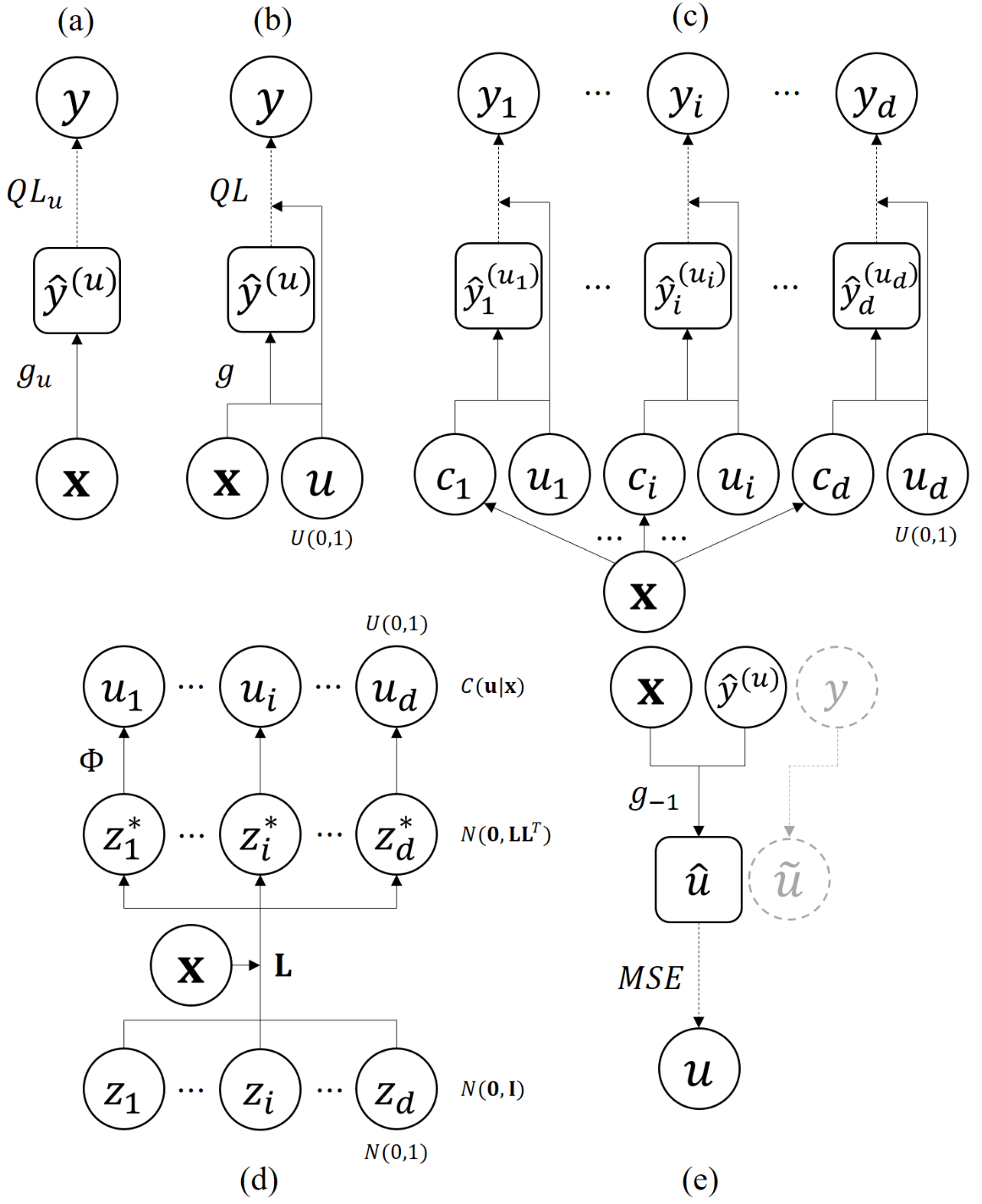
Figure 1: Computational graphs and variable notations used in this paper. Solid arrow indicates forward computation with possibly multiple layers, and dashed arrow is the loss function linking prediction and truth. (a) Quantile Regression; (b) Generative Quantile Model; (c) Generative Multi-Quantile Model with a specific parameterization; (d) Generative conditional Gaussian Copula; (e) Inverse MLP, shown for one target. Grey nodes are the information flow during copula inference. Stacking (c) over (d) leads to the proposed Quantile-Copula model. Notations: we use $\mathbf{y}$ for true targets, $\hat{\mathbf{y}}$ for generated predictions/samples, $\mathbf{x}$/$\mathbf{c}$ for features/contexts, $\mathbf{u}$ for quantile indices of $\hat{\mathbf{y}}$ given $\mathbf{x}$, $\mathbf{z}$ the independent random noises, $\mathbf{z^{*}}$ the associated noises, $\hat{\mathbf{u}}$/$\tilde{\mathbf{u}}$ the estimated quantile indices from $\hat{\mathbf{y}}$/$\mathbf{y}$ given $\mathbf{x}$. See text for detailed discussion.

3 Generative Quantile-Copula Model

We showed in the previous section that both quantile regression and copula modeling can be rephrased as generative models. It is straight-forward to combine them (by stacking Figure 1 (c) over (d)): a copula can convert a set of independent random noises into a correlated and marginally uniform random vector, then a series of quantile functions can be element-wise applied to this vector, interpreted as quantile indices, resulting in a sample conditioned on contexts. Formally, for a random vector pair $(\mathbf{x},\mathbf{y})$, the general Quantile-Copula model is:

$$\mathbf{y}=g_{Q}(\mathbf{u},\mathbf{x})$$

$$\mathbf{u}=g_{C}(\mathbf{z},\theta(\mathbf{x}))$$

where $g_{Q}(\cdot)$ is the multi-target quantile function, $\mathbf{u}$ is the marginal quantile index vector for the corresponding target vector $\mathbf{y}$ given $\mathbf{x}$, $g_{C}(\cdot)$ is the copula generator function, parameterized by $\theta$, to convert independent random noises $\mathbf{z}$ to the desired sample from the copula $C_{\theta}(\mathbf{u}|\mathbf{x})$. Essentially, this is a generator from noise $\mathbf{z}$ to target $\mathbf{y}$ given contexts $\mathbf{x}$, with a layer of intermediate latent variables $\mathbf{u}$ as the quantile indices of each target. In this text, the following parameterization for $g_{Q}$ and $g_{C}$ is used:

$$y_{i}=g(u_{i},c_{i}(\mathbf{x}))\;\forall i$$

$$\mathbf{u}=\Phi(\mathbf{L}(\mathbf{x})\mathbf{z})$$

where $g(\cdot)$ acts as a universal conditional quantile function for all targets, and $c_{i}(\cdot)$ returns target-specific feature embedding as contexts. $\mathbf{L}(\cdot)$ outputs a $d$-by-$d$ lower triangle matrix with a positive diagonal and unit row-norms (so that $\mathbf{L}\mathbf{L}^{\intercal}$ is a correlation matrix) based on $\mathbf{x}$, and $\mathbf{z}\sim N(\mathbf{0},\mathbf{I})$. All functions above are parameterized by either Multi-Layer Perceptrons (MLPs) or structured deep nets (e.g. for time series, $c_{i}(\cdot)$ and $\mathbf{L}(\cdot)$ could be recurrent or convolutional nets over sequential features).

3.1 Learning

The quantile part and the copula part of the model, including their loss functions, are decoupled by the intermediate $\mathbf{u}$. This indicates that we can actually learn the quantile functions first, by drawing $\mathbf{u}$ from independent $U(0,1)$ to pair with each observation. Then the copula can be learned to associate $\mathbf{u}$. This two-phase training is favorable because many applications need the quantile part only and the learning of the more difficult copula part can be stabilized with well initialized quantile functions. For the quantile part, the expected quantile loss needs to be minimized:

$$l_{1}=\mathbb{E}_{(\mathbf{x},\mathbf{y})}\mathbb{E}_{\mathbf{u}}[QL_{\mathbf{u}}(\mathbf{y},\hat{\mathbf{y}})]=\mathbb{E}_{(\mathbf{x},\mathbf{y},\mathbf{u})}[QL_{\mathbf{u}}(\mathbf{y},\hat{\mathbf{y}})]$$

where $\hat{\mathbf{y}}$ is the output of $g_{Q}(\cdot)$ and we abuse the notation of $QL(\cdot)$ as an apply-element-wise-then-sum function. For learning the Gaussian Copula, maximum likelihood is used. A prerequisite of computing the likelihood is to infer the latent variable $\mathbf{u}$ given the truth $\mathbf{y}$. Such reverse mapping can be done efficiently within the neural network. There are two common solutions. One is to enforce invertibility: the choice of neural structure in $g(\cdot)$ is restricted to Flows, a set of invertible layers; the other is to mimic the concept of auto-encoder: if $y_{i}=g(u_{i},c_{i}(\mathbf{x}))$ is an MLP, then a structurally similar inverse MLP $u_{i}=g_{-1}(y_{i},c_{i}(\mathbf{x}))$ can learn this inversion. In this text we pursue the latter because Flows significantly restrict how contexts can be put into the net and thus limit the expressiveness of $g(\cdot)$. Also the inverse MLP works seamlessly in our setting: it can be trained simultaneously with the forward MLP, with the data pairs $(u_{i}\stackrel{{\scriptstyle g}}{{\to}}\hat{y}_{i})$ as ground truths, available for free during the training. See Figure 1 (e). Let $\hat{u}_{i}=g_{-1}(\hat{y}_{i},c_{i}(\mathbf{x}))$, the inverse reconstruction loss is:

$$l_{2}=\mathbb{E}_{(\mathbf{x},\mathbf{y},\mathbf{u})}||\hat{\mathbf{u}}-\mathbf{u}||^{2}$$

Once we have the quantile parts (and its inverse) trained, the weights of the network can be optionally frozen, and the copula part is added to the computation graph. Let the estimated quantile indices for the ground truth be $\tilde{u}_{i}=g_{-1}(y_{i},c_{i}(\mathbf{x}))$, and their corresponding normal score be $\tilde{\mathbf{z}}^{*}=\Phi^{-1}(\tilde{\mathbf{u}})$, then the Gaussian copula can be trained by minimizing the negative log likelihood:

$$l_{3}=\mathbb{E}_{(\mathbf{x},\mathbf{y})}[2\log(|\mathbf{L}|)+(\mathbf{L}^{-1}\tilde{\mathbf{z}}^{*})^{\intercal}(\mathbf{L}^{-1}\tilde{\mathbf{z}}^{*})]+\text{const}$$

In practice, to improve learning stability by allowing better dynamic range, and to avoid the unnecessary use of $\Phi^{-1}(\cdot)$, we actually replace the use of $\mathbf{u}$ by $\mathbf{z}^{*}$: instead of quantile indices themselves, their normal scores are used as both inputs in $g(\cdot)$ and targets in $g_{-1}(\cdot)$, as well as in $l_{2}$. Note $\mathbf{u}=\Phi(\mathbf{z}^{*})$ is still required to be the weights in the QL loss function. $\Phi(\cdot)$ has no analytical form but is known to be well approximated by some polynomials. $\log(|\mathbf{L}|)$ is simply the sum of log diagonal elements of the lower-triangle matrix, and $\mathbf{L}^{-1}\tilde{\mathbf{z}}^{*}$ can be solved by back-substitution for the linear system $\mathbf{L}\tilde{\mathbf{z}}=\tilde{\mathbf{z}}^{*}$; all these operations have symbolic auto-gradient implementations in common deep learning packages, and thus the whole model can be learned using standard gradient-based optimization. There is a numerical instability issue: computing the inverse of $\mathbf{L}(\mathbf{x})$, because during training it may get initialized in an ill-conditioned state, especially when $d$ is large. We use the following empirical guardrail to enforce a stable parameterization of $\mathbf{L}$: output the diagonal and off-diagonal elements of a raw $\mathbf{L}$ separately; clip the diagonal to be greater than 1; put a $\text{tanh}(\cdot)$ activation on off-diagonal; finally divide each row of the raw $\mathbf{L}$ by the row $l^{2}$-norm, so $\mathbf{L}\mathbf{L}^{\intercal}$ is a correlation matrix. This essentially constraints the possible set of correlation matrices that the model can learn, and works well on tested dataset. Although implementing auto-grad regularized matrix inversion or limiting correlation structure would be a formal solution, we describe alternative plans of improvement in Section 5.

3.2 Time Series Modeling

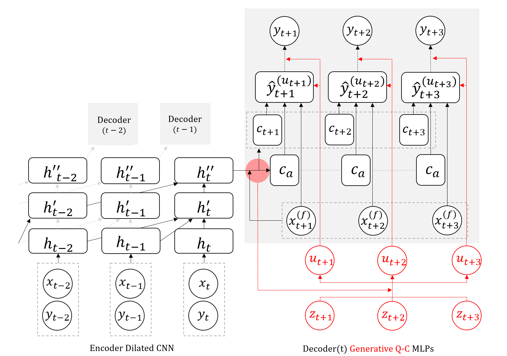
Figure 2: GMQ-Forecaster: Generative Quantile-Copula model (red) applied to MQ-CNN Forecaster (black). The red rounded shade means concatenating all contexts $c_{t:}$, $c_{a}$ and $x_{t:}^{(f)}$ together. Loss functions of Copula and inverse MLPs are not shown for clarity. To generate forecasts, either draw $K$ random $z_{t:}$ to get predictive sample paths of $y_{t:}$ and then infer any quantity of interests using empirical statistics, or set $u_{t:}$ to fixed numbers in $(0,1)$ to directly fetch marginal quantile forecasts for $y_{t:}$.

Wen et al, 2017 formulated probabilistic forecasting as a multi-target regression problem: $p(y_{t+1},\dots,y_{t+d}|\mathbf{x})$, where $\mathbf{x}$ includes past series ($y_{:t}$) and some other historical ($x_{:t}$), static ($x_{s}$), and future available ($x_{t:}^{(f)}$) features. The proposed MQ-forecaster framework uses a sequential net (RNN or 1D CNN) as an encoder to process past temporal features, summarizes them into contexts for each of the $d$ future horizon of interests, and then adopts multiple weight-shared MLPs as decoders to predict quantiles for each horizon. In training, a series of decoders are forked out of each step in the sequential encoder to boost efficiency and stability. The model is trained across all series, with each as a single sample. Since it is a multi-target quantile regression, the generative quantile-copula paradigm can be trivially added to the decoders. See Figure 2.

Probabilistic Forecasting and Simulation This upgrade empowers the MQ-forecaster with the capability to simulate a generative, statistically consistent joint distribution of the future time series (any quantities of interests can be obtained by querying the empirical statistics of a certain number of predictive sample paths), and also to efficiently predict designated marginal quantiles for every $u\in(0,1)$ instead of just the pre-defined ones. The future information $x_{t:}^{(f)}$ (e.g. planned promotion campaigns) can be modified to simulate what-if action scenarios, up to some causal inference configurations. We name the new framework Generative Multivariate Quantile (GMQ-)forecaster.

Cross-series association Note $\tilde{\mathbf{z}}=\mathbf{L}^{-1}\tilde{\mathbf{z}}^{*}$ is the implied independent latent variables (de-correlated white noise) of a given observation series. In the case that there are multiple time series $\mathbf{y}_{j}$, $j=1,\dots,M$, then the $M$-by-$d$ matrix $\tilde{\mathbf{Z}}$ can be used to estimate the copula among the multiple time series (either Gaussian or empirical copula). Such estimation can also accommodate known hierarchical/similarity structure among the series (e.g. demand of substitutable products, inventory units in nearby warehouses), to reduce the dimensionality. Specifically, if the cross-series correlation matrix $\hat{\mathbf{S}}_{M\times M}$ is estimated from $\tilde{\mathbf{Z}}$, subject to regularization and sparsity constraints, then cross-series simulation can be simply achieved by drawing latent variable matrix $\mathbf{Z}_{M\times d}$ so that each column follows $N(\mathbf{0},\hat{\mathbf{S}})$, instead of independently. Then each row of $\mathbf{Z}$ can be fed into the model as before to generate sample paths, and the simulation natively reflects both cross-time and cross-series dynamics.

Anomaly Detection The inverse MLP outputs the implied quantile index $\tilde{\mathbf{u}}$, or its normal score $\tilde{\mathbf{z}}^{*}$, of the observation $\mathbf{y}$. This comes for free and can be conveniently interpreted as a model-based risk score for time series point-anomaly detection and other applications. Likewise, multivariate anomalies (whole series) can be identified from the density of the Gaussian Copula with $\tilde{\mathbf{z}}^{*}$ and $\mathbf{L}$.

4 Experiment: Amazon Demand Forecasting

We apply the GMQ-forecaster to the Amazon Demand Forecasting dataset. 180,000 products are sampled across different categories in the US marketplace, and their weekly demand series are collected from 2014 to 2018. Available covariates include a range of suitably chosen and standard demand drivers in three categories: history only, e.g. past demand units; history and future, e.g. promotions; and static, e.g. product catalog fields. The 3 years of data before 2017 are used to train the models and the rest are for evaluation. Evaluation forecasts are created at each of the 52 weeks in 2017, while each forecast has future horizons from 1 week to 52 weeks.

Before moving into results, we use the next sub-section to explain some pre-requisites and conventions of both modeling and evaluating the joint forecast distribution.

4.1 Mesh, Gamma and Evaluation Metrics

Target Interval and the Mesh Some forecasting applications, like demand forecasting, have a special use case: they require distribution forecasts not only for the time series value in each future horizon, but also for the sum of values in any future intervals (i.e. consecutive horizons). Since quantile is a univariate concept and plain Multi-Quantile nets (e.g. MQ-CNN) only deal with marginals, the Mesh Approach is designed as a work-around to generate distribution forecast for any target intervals: let the maximum horizon length be $d$, then there are $d\times(d-1)/2$ possible intervals $[t+l,t+l+s)\subset[t,t+d]$; pick a moderate subset of supporting $(l,s)$ pairs as the mesh points, and insert these $y_{[t+l,t+l+s)}$ (the total value in the interval) directly as the multi-target of the quantile net, in addition to the horizon targets, so each of them gets quantile forecasts; finally quantile forecasts for any $(l,s)$ outside the mesh points are obtained by interpolating from the nearest three mesh points (triangular interpolation). For example, a mesh of 235 points can be used to interpolate any intervals within the future $d=52$ weeks. Note that, since these mesh points are separate targets to be optimized in the quantile net, there is no guarantee that the probabilistic forecasts would be statistically consistent. For example, it is possible that $\mathbb{E}(\hat{y}_{[t+1,t+2]})\neq\mathbb{E}(\hat{y}_{t+1})+\mathbb{E}(\hat{y}_{t+2})$ or $\hat{y}_{[t+1,t+2]}^{(u)}<\hat{y}_{t+1}^{(u)}$. This causes difficulties if statistical inference on the joint distribution is needed from this set of mesh point quantile forecasts.

Gamma Fitting Quantile nets predict a fixed set of quantiles only. Without the knowledge of Generative Quantile Nets which learn the whole quantile function, previous applications that require full distribution or arbitrary quantiles usually apply interpolation or parametric fitting on the fixed quantile predictions. For example, any demand forecast distribution can be represented by a shifted Gamma distribution. This is essentially a regular Gamma distribution but shifted to the left by 1 unit, and any negative value is considered as 0. This shift is to accommodate the fact that regular Gamma has zero probability to be exactly zero and is not practical for the integer-value demand units of products. A quantile net could generate P50 and P90 quantile forecasts only, and a shifted Gamma fitting procedure estimates the two Gamma parameters from these two quantiles. Then the parametric distribution is stored and used to predict at any quantiles. Such procedure restricts the forecasting distribution to a specific two-parameter family, and cannot implement the multivariate simulation case.

Evaluation Metrics To evaluate the accuracy of a joint forecast distribution for the demand forecast application, we simply follow the same above idea and compute QL on the mesh points. Define $QL_{u}(l,s)$ as the QL of a target interval: $QL_{u}(y_{[t+l,t+l+s)},\hat{y}_{[t+l,t+l+s)}^{(u)})$, where $y_{[a,b)}$ is the total demand units within the time interval $[a,b)$ and $t+1$ is the forecast creation time (the first unknown future point). This can be computed for each $l,s\in\{1,\cdots,d\}$ given $l+s\leq d$. Although any quantiles can be predicted, in this paper a fixed set of $u\in\{0.1,0.3,0.5,0.7,0.9,0.95\}$ is used for evaluation. Note that $QL_{u}(l,1)$ fully characterizes the marginal probabilistic forecast accuracy at each horizon, while $QL_{u}(l,s>1)$ is assessing some representative slices of the joint forecast distribution. In general, the joint distribution or simulation ‘realisticness’ is known to be difficult to quantify, especially for conditional models, and visual examples of samples can be used for intuitive inspection. Apart from the accuracy aspect, to show that MQ-forecaster with Mesh has inconsistencies, we compute the percentage of quantile crossings (Q-X; a lower quantile forecast is greater than a higher one, e.g. $\hat{y}_{t+1}^{(0.9)}<\hat{y}_{t+1}^{(0.7)}$) and interval crossings (I-X; an interval forecast is less than that of a strict subset, e.g. $\hat{y}_{[t+1,t+3)}^{(0.5)}<\hat{y}_{[t+1,t+2)}^{(0.5)}$) in forecast instances.

4.2 Results

In this paper, we do not repeat the state-of-the-art comparisons that already showed the superior accuracy of MQCNN, as listed in Section 1, but instead demonstrate that GMQ can match the accuracy of MQCNN. Candidate models include GMQ-forecaster (GMQ; Quantile-Copula + MQCNN) and two settings of MQCNN: MQ_mesh_gm predicts P50 and P90 forecasts, plus a Gamma fitting, plus the inconsistent Mesh approach, as stated in the previous sub-section; MQ_mesh_6q is similar but directly predict the 6 quantiles being evaluated instead of Gamma fitting. Another new benchmark is the latest development in the field: Autoregressive Implicit Quantile Networks (AIQN; Ostrovski et al, 2018). The AIQN implementation used (Guo, 2018) is tuned for time series forecasting and, like all other candidate models in this experiment, uses exactly the same encoder structure as MQCNN to minimize hyper-parameter confounding. For generative models (GMQ and AIQN), 100 predictive samples are drawn to infer quantiles. Finally, GMQ without copula (GMQ_no_cor) serves as a reference assuming horizon independence, and resembles plain MQ-forecaster without mesh.

Table 1: Experiment Metrics. See texts for explanation.

[]@llrrrrrrrr@ Targets Model P10QL P30QL P50QL P70QL P90QL P95QL Q-X I-X $(l,1)$ MQ_mesh_gm 1.000 1.000 1.000 1.000 1.000 1.000 0.1% N/A MQ_mesh_6q 1.000 1.006 1.006 1.006 1.018 1.024 1.8% N/A GMQ 1.052 1.017 1.003 0.994 1.007 1.023 0% N/A GMQ_no_cor 1.044 1.006 1.001 0.999 1.023 1.085 0% N/A AIQN 1.033 1.110 1.187 1.301 1.661 2.002 0% N/A $(1,s)$ MQ_mesh_gm 1.000 1.000 1.000 1.000 1.000 1.000 0.4% 8.9% MQ_mesh_6q 0.942 0.994 1.005 1.006 1.024 1.030 2.4% 7.2% GMQ 1.013 0.990 0.984 0.986 1.010 1.025 0% 0% GMQ_no_cor 1.653 1.085 0.982 1.019 1.396 1.830 0% 0% AIQN 1.045 1.108 1.208 1.377 1.870 2.302 0% 0%

See Table 1 for evaluation metrics across 180K products and 52 forecast creation times. $(l,1)$: marginal target horizons (averaging all $l$); $(1,s)$: target intervals starting at forecast creation time (averaging all $s$). QL values are scaled by dividing that of MQ_mesh_gm. Q-X and I-X are for quantile crossing and interval crossing percentages (0% is consistent). Q-X is computed between P50/P90 only for MQ_mesh_gm, but across all 6 quantiles for MQ_mesh_6q thus not comparable. For all metrics, the smaller the better. The result shows that MQ and GMQ models have comparable performance, while AIQN falls short, mostly due to underbiased forecasts for longer horizons (not shown). GMQ_no_cor has no ability to model the joint distribution thus fails at $(1,s)$ targets at distribution tails. One surprising fact is that the Gamma-fitted forecasts (MQ_mesh_gm) are as accurate as the nonparametric quantile forecasts (MQ_mesh_6q/GMQ) for this dataset. MQ models have considerable numbers of inconsistent forecasts. Q-crossings can be easily dealt with by sorting, but fixing I-crossings for mesh quantiles is difficult and leave the forecast questionable when inferences are needed, e.g. to compute correlation between horizons. Although metrics of only two types of aggregated target periods are presented, the same conclusion holds for any $(l,s)$ pair.

MQ_mesh models are dedicated to optimize for the mesh, which is only one aspect of the joint distribution. GMQ and AIQN generate sample paths to reflect the full distribution. See Figure 3 for GMQ predictive simulations paths and the corresponding quantile/correlation inference of example products. The marginal quantiles inferred from the 100 sample paths are very close to the direct quantiles by setting $u_{t:}$ to the specific value (not shown; direct quantiles can improve accuracy by 1~2%; also increasing from 100 to 300 samples is another ~1% gain). The conditional copula correlation matrix depends on covariates and is product/time-specific.

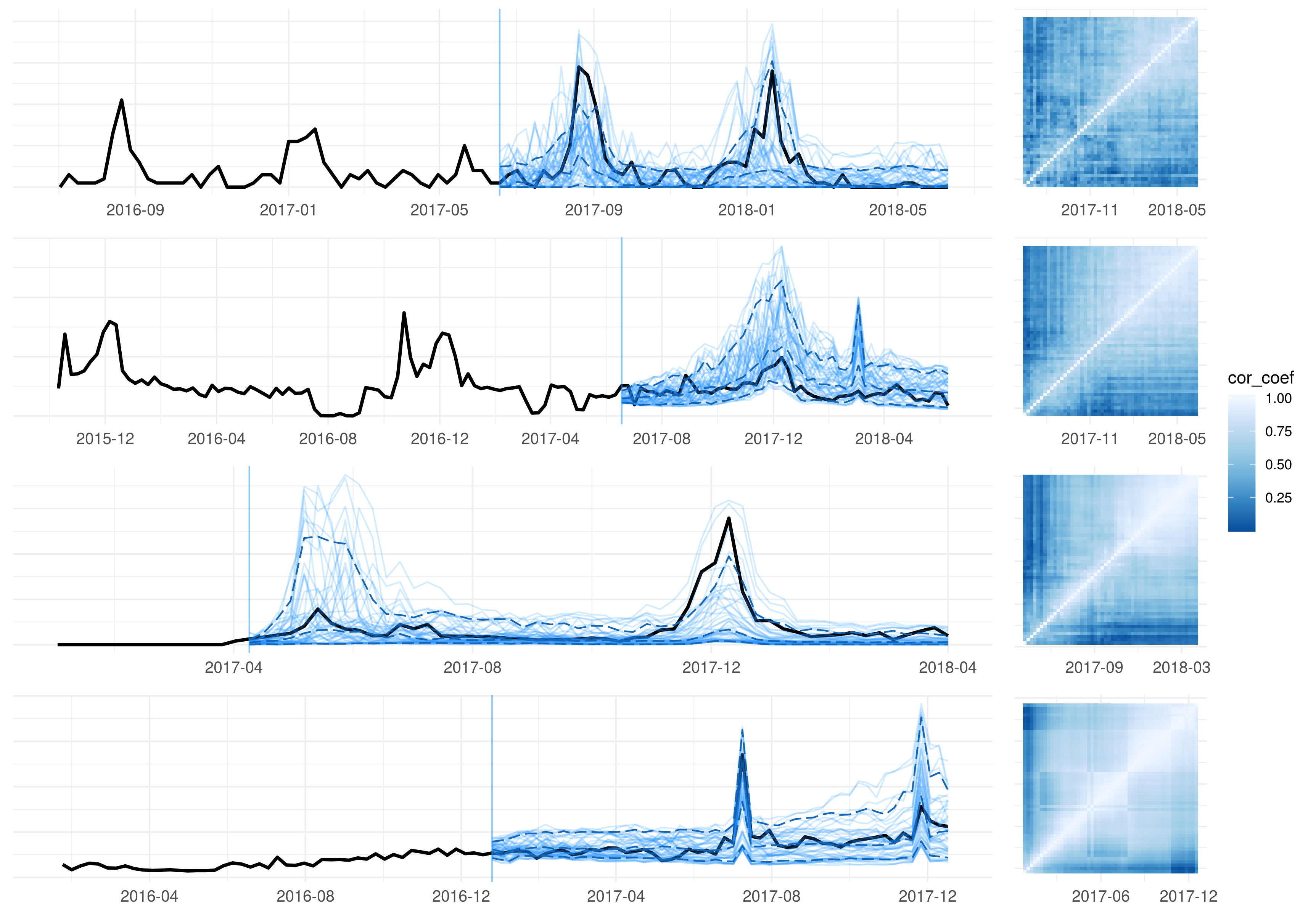
Figure 3: GMQ predictive sample simulations for 4 products. Solid black line is truth; blue vertical line is forecast creation time; solid light blue lines are 100 predictive sample paths, each of length 52 weeks; dashed blue lines are, from lowest to highest, marginal P10/P50/P90 inferred from samples; the horizon-by-horizon Pearson’s correlation matrix is also inferred from samples. The examples are picked to show aspects of double/single seasonality, cold start and future event lifts, respectively.

5 Discussion

Related Work Quantile-Copula decoupling has been well discussed in statistics and forecasting (see Patton, 2012 for a review), but not in the space of deep or generative modeling. Carlier et al, 2016 built a connection between vector quantile regression and the optimal transport problem, but mostly from theoretical aspects. Autoregressive Implicit Quantile Networks (AIQN, Ostrovski et al, 2018) is closely related to our work. AIQN pairs the univariate generative quantile net with an autoregressive model extending to the multivariate case, but suffers all the disadvantages of autoregressive models (e.g. error accumulation). Fan et al, 2016 proposed a trans-normal model by using the empirical marginal quantiles to transform both targets and features into normal scores, then followed by fitting a multivariate Gaussian regression. The trans-normal model assumes simple linear relationship among the transformed features and targets, and cannot model arbitrarily complex interactions. Upon writing this paper, we found another similar work by Toubeau et al, 2019: they used an LSTM-based forecasting model to predict quantiles, and then a separately estimated and stored empirical copula table on a quantile grid/cube to query scenarios. Our work differs by being a single joint deep generative model that characterizes copulas conditioned on different histories and covariates, while theirs assumes an invariant copula under different contexts and depends on the choice of a quantile grid.

Future Work We proposed deep generative Quantile-Copula models, a conditional implicit generative framework that combines the marginally expressive quantile nets and a copula generator. Minimizing marginal quantiles loss enables various applications (e.g. demand forecasting for optimal inventory control), yet the model is general and can be used for any forecasting and simulation application. The framework has much room for extension. Both the quantile part $g_{Q}(\cdot)$ and the copula part $g_{C}(\cdot)$ can be alternatively parameterized by flows-based models. In fact, the Gaussian copula part is a simple one-layer flow, as the ‘invertible $1\times 1$ convolution’ in Glow (Kingma and Dhariwal, 2018). The invertibility of flows would yield more elegant learning and remove the need for inverse MLPs and the Gaussian constraint on copula. This would also help with the possible curse of dimensionality in $d$, where computing the inverse of $\mathbf{L}$ becomes infeasible or not as simple numerically. The major blocker of using flow-based models lies in the lack of well-tested convention to condition on $\mathbf{x}$ while keeping the same level of model expressiveness and thus performance - most previous work is designed for unconditional models. Due to time limit, we leave this extension as well as the applications outside time series data as future work.

Acknowledgment

We would like to thank Fangjian (Richard) Guo for implementing and experimenting the AIQN model on time series.

Reference

Arjovsky, Martin, Soumith Chintala, and Léon Bottou. “Wasserstein gan.” arXiv preprint arXiv:1701.07875 (2017).

Carlier, Guillaume, Victor Chernozhukov, and Alfred Galichon. “Vector quantile regression beyond correct specification.” arXiv preprint arXiv:1610.06833 (2016).

Dinh, Laurent, David Krueger, and Yoshua Bengio. “NICE: Non-linear independent components estimation.” arXiv preprint arXiv:1410.8516 (2014).

Dinh, Laurent, Jascha Sohl-Dickstein, and Samy Bengio. “Density estimation using real nvp.” arXiv preprint arXiv:1605.08803 (2016).

Fan, Jianqing, Lingzhou Xue, and Hui Zou. “Multitask quantile regression under the transnormal model.” Journal of the American Statistical Association 111, no. 516 (2016): 1726-1735.

Flunkert, Valentin, David Salinas, and Jan Gasthaus. “DeepAR: Probabilistic forecasting with autoregressive recurrent networks.” arXiv preprint arXiv:1704.04110 (2017).

Gal, Yarin, and Zoubin Ghahramani. “Dropout as a Bayesian approximation: Insights and applications.” In Deep Learning Workshop, ICML, vol. 1, p. 2. 2015.

Germain, Mathieu, Karol Gregor, Iain Murray, and Hugo Larochelle. “Made: Masked autoencoder for distribution estimation.” In International Conference on Machine Learning, pp. 881-889. 2015.

Gneiting, Tilmann, and Adrian E. Raftery. “Strictly proper scoring rules, prediction, and estimation.” Journal of the American Statistical Association, no. 477 (2007): 359-378.

Goodfellow, Ian, Jean Pouget-Abadie, Mehdi Mirza, Bing Xu, David Warde-Farley, Sherjil Ozair, Aaron Courville, and Yoshua Bengio. “Generative adversarial nets.” In Advances in neural information processing systems, pp. 2672-2680. 2014.

Guo, Fangjian. “Generative modeling of time series via conditional quantiles”. Technical report, SCOT Forecasting, Amazon, 2018.

Kingma, Diederik P., and Max Welling. “Auto-encoding variational bayes.” arXiv preprint arXiv:1312.6114 (2013).

Kingma, Durk P., and Prafulla Dhariwal. “Glow: Generative flow with invertible 1x1 convolutions.” In Advances in Neural Information Processing Systems, pp. 10236-10245. 2018.

Koenker, Roger, and Gilbert Bassett Jr. “Regression quantiles.” Econometrica: journal of the Econometric Society (1978): 33-50.

Madeka, Dhruv, Lucas Swiniarski, Dean Foster, Leo Razoumov, Kari Torkkola, and Ruofeng Wen. “Sample Path Generation for Probabilistic Demand Forecasting.” In KDD MiLeTS workshop, 2018.

Mohamed, Shakir, and Balaji Lakshminarayanan. “Learning in implicit generative models.” arXiv preprint arXiv:1610.03483 (2016).

Oord, Aaron van den, Sander Dieleman, Heiga Zen, Karen Simonyan, Oriol Vinyals, Alex Graves, Nal Kalchbrenner, Andrew Senior, and Koray Kavukcuoglu. “Wavenet: A generative model for raw audio.” arXiv preprint arXiv:1609.03499 (2016).

Ostrovski, Georg, Will Dabney, and Rémi Munos. “Autoregressive quantile networks for generative modeling.” arXiv preprint arXiv:1806.05575 (2018).

Patton, Andrew. “Copula methods for forecasting multivariate time series.” In Handbook of economic forecasting, vol. 2, pp. 899-960. Elsevier, 2013.

Sklar, Abe. “Random variables, joint distribution functions, and copulas.” Kybernetika 9, no. 6 (1973): 449-460.

Toubeau, Jean-François, Jérémie Bottieau, François Vallée, and Zacharie De Grève. “Deep learning-based multivariate probabilistic forecasting for short-term scheduling in power markets.” IEEE Transactions on Power Systems 34, no. 2 (2019): 1203-1215.

Wen, Ruofeng, Kari Torkkola, Balakrishnan Narayanaswamy. “A multi-horizon quantile recurrent forecaster.” In NIPS Time Series Workshop. (2017).

Xu, Qifa, Kai Deng, Cuixia Jiang, Fang Sun, and Xue Huang. “Composite quantile regression neural network with applications.” Expert Systems with Applications 76 (2017): 129-139.