Constant-roll inflation driven by a scalar field
with non-minimal derivative coupling

Abstract

In this work, we study constant-roll inflation driven by a scalar field with non-minimal derivative coupling to gravity, via the Einstein tensor. This model contains a free parameter, $\eta$, which quantifies the non-minimal derivative coupling and a parameter $\alpha$ which characterize the constant-roll condition. In this scenario, using the Hamilton-Jacobi-like formalism, an ansatz for the Hubble parameter (as a function of the scalar field) and some restrictions on the model parameters, we found new exact solutions for the inflaton potential which include power-law, de Sitter, quadratic hilltop and natural inflation, among others. Additionally, a phase space analysis was performed and it is shown that the exact solutions associated to natural inflation and a “$\cosh$-type” potential, are attractors.

PACS numbers: 98.80.Cq, 98.80.-k, 04.50.Kd

1 Introduction

Inflation is a stage of the early universe in which it exhibits a quasi-de Sitter phase during a very short time ($\sim 10^{-33}\,s$) and at very high energy scales ($\sim 10^{16}\,eV$) after the Big Bang. The inflationary paradigm is currently considered as a part of the standard modern cosmology. This paradigm was introduced in the early 1980’s to resolve some problems that the Hot Big Bang model of the universe can’t explain (e.g., the horizon, the flatness, and the monopole problems, among others) [1, 2, 3, 4]. On the other hand, inflation makes predictions about properties of the current universe which have been confirmed by numerous cosmological and astrophysical observations (e.g., the temperature fluctuations in CMB spectrum [5, 6, 7], the existence of large scale structures [8, 9, 10, 11], and the nearly scale invariant primordial power spectrum [12, 13, 14]).

The simplest scenario to explain the dynamics of inflation consists of introducing a single scalar field (dubbed inflaton) minimally coupled to gravity and with a nearly flat potential, namely, the potential energy of the field dominates over their kinetic term. Under this condition, it has the so-called slow-roll inflation (for more details about this topic see Refs. 15 and 16). On the other hand, it is also possible to consider the inflaton non-minimally coupled to gravity via the Ricci scalar, the Ricci tensor, the Gauss-Bonnet invariant, etc, which have been widely studied in the literature in distinct scenarios. All these theories (with minimal or non-minimal couplings to gravity) are known as scalar-tensor theories of gravitation (see e.g. Ref. 17 for a review). In this context, the most general scalar-tensor theory that produces second-order equations of motion was found by Horndeski [18]. A subclass of the Horndeski models, are theories in which the non-minimal derivative coupling (NMDC) with the Einstein tensor is taken into account. But, at present, these theories are not good candidates to explain dark energy (DE), since the detection of an electromagnetic counterpart (GRB 170817A) to the gravitational wave signal (GW170817) from the merger of two neutron stars, showed that the speed of gravitational waves (GW) $c_{t}$ is the same as the speed of light, within deviations of order $10^{-15}$ for the redshift $z<0.009$ (see Refs. 19 and 20). Contrary to this result, the theories with NMDC predict a variable GW speed at low redshift. In general, the above imposes stringent constraints on dark energy models constructed in the framework of scalar-tensor and vector-tensor theories. Nevertheless, this restriction does not apply to high redshift values, thus, these scalar-tensor theories with NMDC could be used in an inflationary context (for a recent review about this topic see Ref. 21). In the literature, there are several works on inflation with a NMDC. [22, 23, 24, 25, 26] Usually, these models have been studied in the context of slow-roll inflation (see e.g. Refs. 27 and 28 for more details), but in the last years, a new route has been considered in the literature instead of slow-roll inflation. In this new scenario, the slow-roll inflation is replaced by the more general, constant-roll condition. In these models the scalar field $\phi$ is assumed to satisfy the constant-roll condition $\ddot{\phi}=-(3+\alpha)H\dot{\phi}$, where $H$ is the Hubble parameter and $\alpha$ is an arbitrary constant. one can see that the usual slow-roll inflation occurs if $\alpha=-3$ while the “ultra-slow-roll” case corresponds to $\alpha=0$. Constant-roll inflation was originally introduced in Ref. 29 and recently it attracted a lot of interest [30, 31, 32, 33, 34, 35, 36, 37, 38, 39, 40, 41, 42].

In this work we use the constant-roll condition in a model of inflation with NMDC to the Einstein tensor, we also use the Hamilton-Jacobi-like formalism, an ansatz for the Hubble parameter (as a function of the scalar field) and some restrictions on the model parameters. From the above, we find new exact solutions for the inflaton potential.

This paper it is organized as follows: in section 2 we introduce the scalar-tensor model of inflation with non-minimal derivative coupling to gravity, via the Einstein tensor, and the corresponding field equations are obtained. In section 3, we consider a flat FRW universe and a homogeneous scalar field, and from these considerations, general expressions for the equation of motion and the total energy momentum tensor are obtained. In section 3 we consider the constant-roll condition and we use the Hamilton-Jacobi-like formalism, an ansatz for the Hubble parameter (as a function of the scalar field) and some restrictions on the model parameters, to find new exact solutions for the inflaton potential. In section 4 we realize a phase space analysis, and some conclusions are exposed in section 5.

2 The model

The action for the scalar field with the kinetic term non-minimally coupled to Einstein tensor is

$$S=\int{{d}^{4}x\sqrt{-g}\left(\frac{{M}_{pl}^{2}}{2}R-\frac{1}{2}{g}^{\mu\nu}{\partial}_{\mu}\phi{\partial}_{\nu}\phi-V(\phi)+\eta\,{G}_{\mu\nu}{\partial}^{\mu}\phi{\partial}^{\nu}\phi\right)},$$ (1)

where $M^{2}_{\text{pl}}=(8\pi G)^{-1}$ is the reduced Planck mass, $g_{\mu\nu}$ is the metric tensor, $G_{\mu\nu}={R}_{\mu\nu}-\frac{1}{2}{g}_{\mu\nu}R$ is the Einstein tensor, $\eta$ is a coupling constant with dimensions $M^{-2}$ and $V(\phi)$ is a potential term.

Models with a NMDC similar to Eq. (1) have been widely studied in the literature in a cosmological and astrophysical context [43, 44, 45, 46, 47]. In cosmology, usually, they have been used to explain inflation and dark energy problems. However, recently these models have been discarded in the context of dark energy, since they predict a variable GW speed at low redshift (which is contrary to the gravitational waves measurements lately realized [19, 20]). In the inflationary context, there are several works on inflation with a NMDC, for example, in Ref. shinji, the author studied observational constraints on a number of representative inflationary models with a field derivative coupling to the Einstein tensor. In Refs. gao1 and gao2 the authors derive the general formulae for the the scalar and tensor spectral tilts to the second order for the inflationary models with NMDC taking into account high friction limit and without it. In Ref. myung, the authors investigate the slow-roll inflation in the NMDC model with exponential, quadratic, and quartic potentials. Finally, in Ref. saridakis the authors investigate inflation with NMDC through the Hamilton-Jacobi formalism.

The variation of the action, Eq. (1), with respect to the metric tensor $g_{\mu\nu}$ gives the field equations

$${R}_{\mu\nu}-\frac{1}{2}{g}_{\mu\nu}R=\frac{1}{{M}_{pl}^{2}}{T}_{\mu\nu},\hskip 22.76228pt{T}_{\mu\nu}={T}_{\mu\nu}^{(\phi)}+\eta\hskip 1.13791pt{\Theta}_{\mu\nu},$$ (2)

where ${T}_{\mu\nu}^{(\phi)}$ and ${\Theta}_{\mu\nu}$ are given by

$${{T}_{\mu\nu}^{(\phi)}}={\nabla}_{\mu}\phi{\nabla}_{\nu}\phi-{g}_{\mu\nu}\Big{(}{\nabla}^{\alpha}\phi{\nabla}_{\alpha}\phi+V(\phi)\Big{)},$$ (3)

$${\Theta}_{\mu\nu}= \hskip 1.70709pt{G}_{\mu\nu}{\nabla}^{\alpha}\phi{\nabla}_{\alpha}\phi+{g}_{\mu\nu}\Big{(}{R}^{\alpha\beta}{\nabla}_{\alpha}\phi{\nabla}_{\beta}\phi+\Box\left({\nabla}^{\alpha}\phi{\nabla}_{\alpha}\phi\right)-{\nabla}^{\alpha}{\nabla}^{\beta}\left({\nabla}_{\alpha}\phi{\nabla}_{\beta}\phi\right)\Big{)}+R{\nabla}_{\mu}\phi{\nabla}_{\nu}\phi$$

$$+2{\nabla}_{\alpha}{\nabla}_{(\mu}\left({\nabla}_{\nu)}\phi{\nabla}^{\alpha}\phi\right)-4{R}_{\alpha(\mu}{\nabla}_{\nu)}\phi{\nabla}^{\alpha}\phi-{\nabla}_{\nu}{\nabla}_{\mu}\left({\nabla}^{\alpha}\phi{\nabla}_{\alpha}\phi\right)-\square\left({\nabla}_{\mu}\phi{\nabla}_{\nu}\phi\right).$$ (4)

On the other hand, the variation of the action with respect to the scalar field, gives the equation of motion

$$-\square\left(\phi\right)+\frac{\partial V}{\partial\phi}+2\eta{\nabla}_{\mu}\left({R}^{\mu\nu}{\partial}_{\nu}\phi\right)-\eta{\nabla}_{\mu}\left({R}{\partial}^{\mu}\phi\right)=0.$$ (5)

3 Constant-roll inflation with NMDC

In this section we use the constant-roll condition in the background equations obtained in the previous section. To this aim, the first step is to consider a flat, homogeneous and isotropic universe whose metric is given by Friedmann-Robertson-Walker (FRW) metric:

$$ds^{2}=-dt^{2}+a(t)^{2}\delta_{ij}dx^{i}dx^{j},$$ (6)

where $a(t)$ is the scale factor. Using in Eqs. (2) and (5), the FRW metric and considering that the scalar field is homogeneous ($\phi\equiv\phi(t)$), we obtain the Friedmann equations

$$3{M}_{pl}^{2}{H}^{2}=\frac{1}{2}{\dot{\phi}}^{2}+V\left(\phi\right)+9\eta{H}^{2}{\dot{\phi}}^{2},$$ (7)

$$-2{M}_{pl}^{2}\dot{H}={\dot{\phi}}^{2}+6\eta{H}^{2}{\dot{\phi}}^{2}-2\eta\dot{H}{\dot{\phi}}^{2}-4\eta H\dot{\phi}\ddot{\phi},$$ (8)

and the scalar field equation

$$\ddot{\phi}+3H\dot{\phi}+\frac{dV}{d\phi}+12\eta H\dot{H}\dot{\phi}+6\eta{H}^{2}\ddot{\phi}+18\eta{H}^{3}\dot{\phi}=0,$$ (9)

where a dot denotes differentiation with respect to cosmic time $t$.

Usually, to solve the system of equations (7)-(9) in an inflationary context, it’s a common practice to use the slow-roll parameters defined as

$$\epsilon\equiv-\frac{\dot{H}}{H^{2}},$$ (10)

$$\delta\equiv-\frac{\ddot{\phi}}{H\dot{\phi}},$$ (11)

which control the inflationary dynamics. Additionally, the slow-roll conditions $|\epsilon|\ll 1$ and $|\delta|\ll 1$ are imposed. In this work, let’s consider that the second slow-roll condition is violated. In this sense, we use the constant-roll condition given by [30]

$$\ddot{\phi}=-\left(3+\alpha\right)H\dot{\phi},$$ (12)

where $\delta\equiv 3+\alpha$ and $\alpha$ an arbitrary constant. In order to solve the system of equations (7)-(9) with the condition (12), we consider the Hubble parameter as a function of the inflaton field $H=H(\phi)$ and use the Hamilton-Jacobi-like formalism [30]. Thereby, since $\dot{H}=\dot{\phi}\,{dH}/{d\phi}$, and using Eq. (12), we can rewrite (8) as

$$-2{M}_{pl}^{2}\frac{dH}{d\phi}=\dot{\phi}\left(1+6\eta{H}^{2}\right)-2\eta\frac{dH}{d\phi}{\dot{\phi}}^{2}+4\eta\left(\alpha+3\right){H}^{2}\dot{\phi},$$ (13)

which can be solved with respect to $\dot{\phi}$, so that

$$\dot{\phi}=\frac{1+2\left(9+2\alpha\right)\eta{H}^{2}\pm\sqrt{{\Big{(}1+2\left(9+2\alpha\right)\eta{H}^{2}\Big{)}}^{2}+16{M}_{pl}^{2}\eta\left(\frac{dH}{d\phi}\right)^{2}}}{4\eta\frac{dH}{d\phi}}.$$ (14)

Notice that in Eq. (14) there are two possible solutions to $\dot{\phi}$. In this case, the right solution corresponds to the negative sign (since for $\eta=0$ the present model is reduced to the model analyzed in Ref. motohashi1).

Differentiating Eq. (14) with respect to $t$ and using Eq. (12), we obtain

$$12\left(4+\alpha\right)H+\frac{\left[-1-2\left(9+2\alpha\right)\eta{H}^{2}+f(\phi)\right]\frac{d^{2}H}{d\phi^{2}}}{\eta\left(\frac{dH}{d\phi}\right)^{2}}$$

$$-\frac{4\left[\left(9+2\alpha\right)H+2{\left(9+2\alpha\right)}^{2}\eta{H}^{3}+4{M}_{pl}^{2}\frac{d^{2}H}{d\phi^{2}}\right]}{f(\phi)}=0,$$ (15)

where, for simplicity, we have defined $f(\phi)\equiv\sqrt{{\left[1+2\left(9+2\alpha\right)\eta{H}^{2}\right]}^{2}+16{M}_{pl}^{2}\eta\left(\frac{dH}{d\phi}\right)^{2}}$. It is evident that this non-linear differential equation for $H(\phi)$ is very complicated, and finding exact solutions for it is a hard task. Nevertheless, we know that for $\eta=0$, Eq. (13) is reduced to

$$-2{M}_{pl}^{2}\frac{dH}{d\phi}=\dot{\phi},$$ (16)

in this case, Eq. (3) becomes

$$\frac{{d}^{2}H}{d{\phi}^{2}}=\frac{3+\alpha}{2{M}_{pl}^{2}}H,$$ (17)

and the general solution of this equation is

$$H\left(\phi\right)={C}_{1}\hskip 1.42271pt\textrm{exp}\left(\sqrt{\frac{3+\alpha}{2}}\frac{\phi}{{M}_{pl}}\right)+{C}_{2}\hskip 1.42271pt\textrm{exp}\left(-\sqrt{\frac{3+\alpha}{2}}\frac{\phi}{{M}_{pl}}\right).$$ (18)

which was found in Ref. motohashi1. Inspired by this solution, the authors in Ref. ito propose the following ansatz:

$$H(\phi)={C}_{1}\hskip 1.42271pt\textrm{exp}\left(\lambda\left(n\right)\sqrt{\frac{3+\alpha}{2}}\frac{\phi}{{M}_{pl}}\right)+{C}_{2}\hskip 1.42271pt\textrm{exp}\left(-\lambda\left(n\right)\sqrt{\frac{3+\alpha}{2}}\frac{\phi}{{M}_{pl}}\right).$$ (19)

In a similar way, we will use this ansatz at the present model (changing $n$ by $\eta$).

Replacing the ansatz (19) in Eq. (3) and after some simplifications, we obtain the following system of algebraic equations:

$${C}_{1}\eta\lambda(\alpha+3)(\alpha+4)(2\alpha+9)=0,$$ (20)

$${C}_{1}\eta\lambda(\alpha+3)\Big{[}8\alpha^{2}+(4\alpha+15)^{2}\lambda^{2}+66\alpha-4(\alpha+6)(2\alpha+9)^{2}{C}_{1}{C}_{2}\eta+135\Big{]}=0,$$ (21)

$${C}_{1}\eta\lambda(\alpha+3)\Big{[}8\alpha\lambda^{2}+\alpha+30\lambda^{2}+6+656\alpha^{3}{C}_{1}^{2}{C}_{2}^{2}\eta^{2}+16\alpha^{2}{C}_{1}{C}_{2}\eta(549{C}_{1}{C}_{2}\eta+16\lambda^{2}+6)$$ (22)

$$+36\alpha{C}_{1}{C}_{2}\eta(1089{C}_{1}{C}_{2}\eta+56\lambda^{2}+24)+72{C}_{1}{C}_{2}\eta(810{C}_{1}{C}_{2}\eta+55\lambda^{2}+27)\Big{]}=0,$$

$${C}_{1}\eta\lambda(\alpha+3)\Big{[}\Big{(}4(2\alpha+9){C}_{1}{C}_{2}\eta+1\Big{)}^{2}\Big{(}4(7\alpha+30){C}_{1}{C}_{2}\eta+1\Big{)}-$$ (23)

$$\Big{(}4(8\alpha+33){C}_{1}{C}_{2}\eta\lambda+\lambda\Big{)}^{2}\Big{]}=0,$$

$${C}_{1}{C}_{2}\eta\lambda(\alpha+3)\Big{[}8\alpha\lambda^{2}+\alpha+30\lambda^{2}+6+608\alpha^{3}{C}_{1}^{2}{C}_{2}^{2}\eta^{2}+32\alpha^{2}{C}_{1}{C}_{2}\eta(255{C}_{1}{C}_{2}\eta+$$ (24)

$$8\lambda^{2}+3)+72\alpha{C}_{1}{C}_{2}\eta(507{C}_{1}{C}_{2}\eta+28\lambda^{2}+12)+72{C}_{1}{C}_{2}\eta(756{C}_{1}{C}_{2}\eta+55\lambda^{2}+27)\Big{]}=0,$$

$${C}_{1}{C}_{2}\eta\lambda(\alpha+3)\Big{[}16(2\alpha+9)^{2}(29\alpha+126){C}_{1}^{3}{C}_{2}^{3}\eta^{3}+4{C}_{1}{C}_{2}\eta(-2(8\alpha+33)\lambda^{2}+$$ (25)

$$11\alpha+48)-\lambda^{2}+1+4{C}_{1}^{2}{C}_{2}^{2}\eta^{2}\Big{(}3(2\alpha+9)(20\alpha+87)-(8\alpha(34\alpha+279)+4581)\lambda^{2}\Big{)}\Big{]}=0.$$

The solutions of the system (20)-(25) are:

1. $\{C_{1}=0\}$

2. $\{\alpha=-3\}$

3. $\{\lambda=0\}$

4. $\{C_{2}=0,\ \ \lambda=\pm 1,\ \ \alpha=-4\}$

5. $\{\lambda=\pm\sqrt{1+8C_{1}C_{2}\eta},\ \ \alpha=-4\}$

We now proceed to analyze the above solutions.

3.1 Solution (a) $\{C_{1}=0\}$

In this case Eq. (19) reduces to

$$H(\phi)=Me^{-\lambda(\eta)\sqrt{\frac{3+\alpha}{2}}\frac{\phi}{{M}_{pl}}},$$ (26)

where the choice $C_{2}=M$ was made (the mass $M$ determines both the energy scale at which inflation occurs and the amplitude of the primordial fluctuations). Besides, in Eq. (26), $\lambda(\eta)$ and $\alpha$ are arbitrary quantities. In this case, for $\alpha<-3$ and $\lambda(\eta)$ a real number, the solution (26) has not physical meaning. Conversely, for $\alpha>-3$ and $\lambda(\eta)$ a real number, the solution (26) is viable, and from Eq. (7), we obtain

$$V(\phi)=3M^{2}M_{\text{pl}}^{2}e^{2\beta\phi/M_{\text{pl}}}-$$ (27)

$$\frac{M^{2}e^{-2\beta\phi/M_{\text{pl}}}\left(1+18\gamma e^{2\beta\phi/M_{\text{pl}}}\right)\left[\sqrt{1+4\gamma e^{2\beta\phi/M_{\text{pl}}}\left(1+4\beta^{2}M_{\text{pl}}^{2}+\gamma e^{2\beta\phi/M_{\text{pl}}}\right)}-1-2\gamma e^{2\beta\phi/M_{\text{pl}}}\right]^{2}}{32\beta^{2}\gamma^{2}},$$

where $\gamma\equiv M^{2}\eta$ is a dimensionless parameter and $\beta=-\lambda(\eta)\sqrt{\frac{3+\alpha}{2}}$. For suitable values of the model parameters, the potential (27) represents a power-law-type inflation (see Fig. 1). In addition, if $\eta\rightarrow 0$ and $\lambda=-1$, we have the power-law potential reported in Ref. motohashi1, but it is ruled out by the authors (since it does not satisfy the observational constraints). In Ref. shinji the author studied observational constraints on a number of representative inflationary models with NMDC, and in particular, he showed that exponential potentials (i.e., $V(\phi)=V_{0}e^{\beta\phi/M_{\text{pl}}}$, where $V_{0}$ and $\beta$ are constants) can be made compatible with the current observational data. However, in our case the potential (27) is more complicate and it would be necessary to investigate the most recent observational constraints on model parameters.

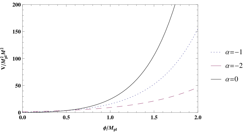
Figure 1: Potential versus scalar field, using $\gamma=1$, $\lambda=-1$ and three different values for $\alpha$: $\alpha=-1$ (dotted line), $\alpha=-2$ (dashed line) and $\alpha=0$ (solid line).

3.2 Solutions (b) $\{\alpha=-3\}$ and (c) $\{\lambda=0\}$

Continuing with the analysis, Eq. (19) reduces to a constant and therefore these solutions represent the de Sitter universe.

3.3 Solution (d) $\{C_{2}=0,\ \ \lambda=\pm 1,\ \ \alpha=-4\}$

In this case Eq. (19) has not physical meaning.

3.4 Solution (e) $\{\lambda=\pm\sqrt{1+8C_{1}C_{2}\eta},\ \ \alpha=-4\}$

This solution is more interesting. In this case, considering the positive sign in $\lambda$, Eq. (19) takes the form

$$H(\phi)=C_{1}e^{i\lambda(\eta)\frac{\sqrt{2}}{2}\frac{\phi}{M_{\text{pl}}}}+C_{2}e^{-i\lambda(\eta)\frac{\sqrt{2}}{2}\frac{\phi}{M_{\text{pl}}}},$$ (28)

where $\lambda(\eta)=\sqrt{1+8C_{1}C_{2}\eta}$. An identical result is obtained using the negative sign for $\lambda$. Now, we consider the case $C_{1}=C_{2}={M}/{2}$ (a similar consideration was carried out in Refs. motohashi1 and ito), then (28) becomes

$$H(\phi)=M\cos{\left(\frac{\sqrt{2}}{2}\sqrt{1+2\gamma}\frac{\phi}{M_{\text{pl}}}\right)},$$ (29)

where the restriction $1+2\gamma>0$ (or $\gamma>-\frac{1}{2}$) has been considered.

The potential $V(\phi)$ is obtained replacing Eqs. (14) and (28) in Eq. (7), so that

$$V(\phi)= \frac{M^{2}M_{\text{pl}}^{2}}{4\left(1+2\gamma\right)}\Bigg{[}4+3\gamma+4(2+3\gamma)\cos{\left(\sqrt{2(1+2\gamma)}\frac{\phi}{M_{\text{pl}}}\right)}+$$ (30)

$$9\gamma\cos{\left(2\sqrt{2(1+2\gamma)}\frac{\phi}{M_{\text{pl}}}\right)}\Bigg{]}.$$

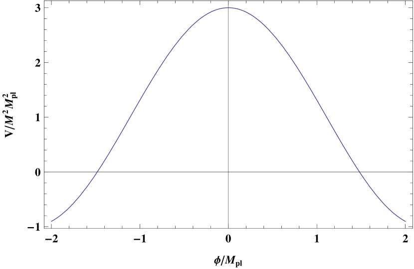
Figure 2: Potential versus scalar field, using $\gamma=10^{-9}$ in Eq. (30).

The potential (30) represents a general case of natural inflation (see Fig. 2). Considering $\phi$ near to origin, the potential (30) reduces to hilltop inflation [48], namely

$$V(\phi)\approx 3M^{2}M_{\text{pl}}^{2}-2M^{2}\left(1+6\gamma\right)\phi^{2},$$ (31)

and to guarantee the hilltop inflation, $1+6\gamma>0$. Additionally, in Ref. motohashi1 the authors showed that a similar model to that given by Eq. (30) is observationally viable.

In other words, replacing Eq. (29) in Eq. (14), we obtain

$$\phi(t)=\frac{2\sqrt{2}}{\sqrt{1+2\gamma}}M_{\text{pl}}\,\text{arctan}{\left(e^{Mt}\right)}.$$ (32)

The integration constant that arises in (32) has been removed, since its contribution does not change the form of the function $\phi(t)$. But, in general, $t$ must be replaced by $t+\frac{\sqrt{2(1+2\gamma)}}{2MM_{\text{pl}}}C$, where $C$ is the integration constant. Using Eq. (32) in Eq. (29), we get

$$H(t)=-M\tanh(Mt),$$ (33)

from the defnition $H=\dot{a}/a$, we have

$$a(t)\propto\text{sech}(Mt).$$ (34)

Additionally $\ddot{a}(t)>0$, so the model can describe an inflationary regimen. Eqs. (32)-(34) are similar (taking $\alpha=-4$) to those reported in Ref. motohashi1. It is easy to check that if $Mt\rightarrow-\infty$ then $(\phi(t),\dot{\phi}(t))\rightarrow(0,0)$ and $H\rightarrow M$, which guarantees that these functions exhibit a good behavior under these conditions (i.e. are bounded functions).

On the other hand, for $1+2\gamma<0$ (which implies that $\gamma<-\frac{1}{2}$), the “$\cos$” function must be replaced by “$\cosh$” and $1+2\gamma$ by $|1+2\gamma|$ in Eq. (29), namely

$$H(\phi)=M\cosh{\left(\frac{\sqrt{2}}{2}\sqrt{|1+2\gamma|}\frac{\phi}{M_{\text{pl}}}\right)}.$$ (35)

The potential $V(\phi)$ is

$$V(\phi)= \frac{M^{2}M_{\text{pl}}^{2}}{4(1+2\gamma)}\Bigg{[}4+3\gamma+4(2+3\gamma)\cosh{\Bigg{(}\sqrt{2|1+2\gamma|}\frac{\phi}{M_{\text{pl}}}\Bigg{)}}$$ (36)

$$+9\gamma\cosh{\Bigg{(}2\sqrt{2|1+2\gamma|}\frac{\phi}{M_{\text{pl}}}\Bigg{)}}\Bigg{]},$$

and

$$\phi(t)=\frac{2\sqrt{2}}{\sqrt{|1+2\gamma|}}M_{\text{pl}}\,\text{arctanh}{\left(e^{Mt}\right)},$$ (37)

$$H(t)=M\cosh[2\,\text{arctanh}\left(e^{Mt}\right)],$$ (38)

$$a(t)\propto\text{csch}(Mt).$$ (39)

Also, in this case $\ddot{a}(t)>0$ and in general, $t\rightarrow t+\frac{\sqrt{2|1+2\gamma|}}{2MM_{\text{pl}}}C$. Again, if $Mt\rightarrow-\infty$ then $(\phi(t),\dot{\phi}(t))\rightarrow(0,0)$ and $H\rightarrow M$. In Fig. 3 we can see the potential given by Eq. (36).

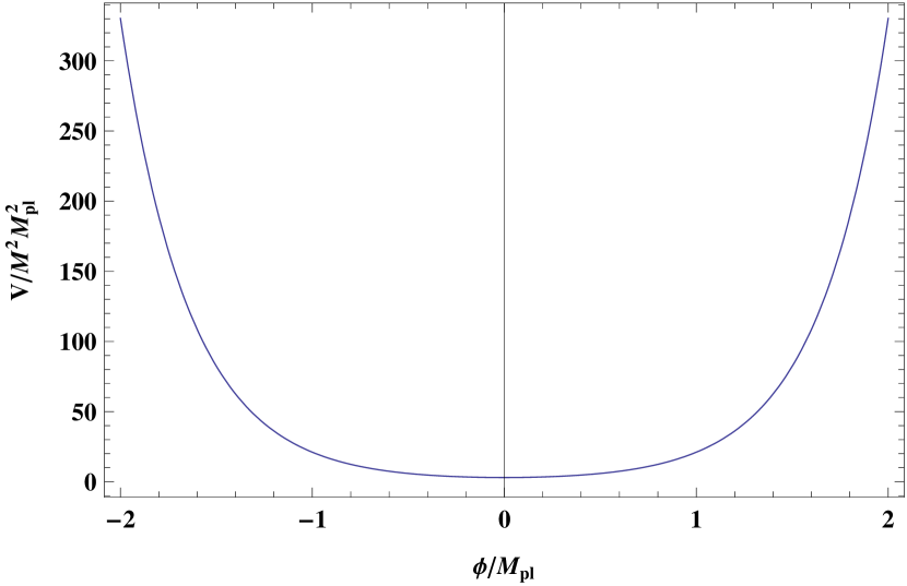
Figure 3: Potential versus scalar field, using $\gamma=-1$ in Eq. (36).

Next, we consider the choice $C_{1}=M/2$ and $C_{2}=-M/2$ in Eq. (28). In this case, for $1-2\gamma>0$ (or $\gamma<\frac{1}{2}$) the solution is not physical. For $1-2\gamma<0$ (or $\gamma>\frac{1}{2}$) and taking into account that $\lambda=\pm\sqrt{|1-2\gamma|}$, Eq. (28) is reduced to

$$H(\phi)=\mp M\sinh{\left(\frac{\sqrt{2}}{2}\sqrt{|1-2\gamma|}\frac{\phi}{M_{\text{pl}}}\right)}.$$ (40)

The potential is

$$V(\phi)= \frac{M^{2}M_{\text{pl}}^{2}}{4\gamma^{2}}\Bigg{[}6\gamma\Bigg{(}3-7\gamma+\gamma\,\text{cosh}\Bigg{(}\sqrt{2|1-2\gamma|}\frac{\phi}{M_{\text{pl}}}\Bigg{)}\Bigg{)}$$ (41)

$$+(1-4\gamma(5-9\gamma))\text{sech}^{2}\Bigg{(}\frac{\sqrt{2|1-2\gamma|}}{2}\frac{\phi}{M_{\text{pl}}}\Bigg{)}\Bigg{]},$$

which is valid for both signs of Eq. (40). On the other hand, for the positive sign in (40), we get

$$\phi(t)=\mp\frac{\sqrt{2}}{\sqrt{|1-2\gamma|}}M_{\text{pl}}\,\text{arcsinh}{\left[\pm Mt\left(1-\frac{1}{2\gamma}\right)\right]},$$ (42)

and for the negative sign, we obtain

$$\phi(t)=\pm\frac{\sqrt{2}}{\sqrt{|1-2\gamma|}}M_{\text{pl}}\,\text{arcsinh}{\left[\pm Mt\left(1-\frac{1}{2\gamma}\right)\right]},$$ (43)

and by last

$$H(t)=M^{2}t\left(1-\frac{1}{2\gamma}\right),$$ (44)

$$a(t)\propto\exp{\left[\frac{M^{2}t^{2}}{2}\left(1-\frac{1}{2\gamma}\right)\right]}.$$ (45)

which are valid for both signs.

Now, if $Mt\rightarrow\pm\infty$ then $(\phi(t),\dot{\phi}(t))\rightarrow(\pm\infty,0)$ and $H\rightarrow\pm\infty$. Therefore, the functions $\phi$ and $H$ do not present a good behavior under these conditions, and so, the solution Eq. (40) is not viable in this context.

4 Analysis of the phase space

Now we proceed to verify whether the solutions given by Eqs. (29) and (35) are attractors solutions or not (the same formalism can be used for the other solutions). In this ways, we numerically solved Eqs. (7)-(9) under the assumption (12) and also, we used the potentials $V(\phi)$ found for each case. In this sense, the first case studied was the solution given by Eq. (29). Additionally, various initial conditions were considered for it (for simplicity, only four choices are shown). Thereby, we obtained the phase space diagram shown in Fig. 4, in which, we see that the phase space flow converge in distinct points depending on initial conditions. This observed pattern is related to the form of the potential (30), since it is a periodic function of $\phi$ and it preserves its form under the translation $\phi\rightarrow\phi+\text{const.}$ (a similar result was obtained in Ref. motohashi1, for $\alpha=0$). Besides, an analogous behavior it is obtained using other initial conditions and suitable values for the model parameters. For the solution (35), as $\phi$ and $\dot{\phi}$ are not defined in $t=0$, it’s necessary to recover the integration constant in the analytic solution given by Eq. (37), (i.e. $t\rightarrow t+\frac{\sqrt{2(1+2\gamma)}}{2MM_{\text{pl}}}C$), and determine it according to an arbitrary initial condition. So, in Fig. 5 we display the phase space diagram associated to the solution given by Eq. (35), in which we see a typical attractor behavior where the trajectories converges to $\phi=0$ and $\dot{\phi}=0$. This implies that the inflaton approaches to the global minimum of the potential at $\phi=0$ (see Fig. 3). Furthermore, for various initial conditions and for small values of the variables $(\phi,\dot{\phi})$, all trajectories overlap. The trajectories are separated for larger values of the variables. By last, the inflationary solutions studied above, fulfill the first slow-roll condition $|\epsilon|\ll 1$ (see Fig. 6).

Figure 4: Phase space structure of the solution (29). In this numerical simulation we have used: from left to right $\frac{\phi_{0}}{M_{\text{pl}}}=5$, $\frac{\phi_{0}}{M_{\text{pl}}}=10$, $\frac{\phi_{0}}{M_{\text{pl}}}=15$, $\frac{\phi_{0}}{M_{\text{pl}}}=20$ and $\gamma=10^{-3}$.

Figure 5: Phase space structure of the solution (35). In this numerical simulation we have used: $\frac{\phi_{0}}{M_{\text{pl}}}=5$ (right top plot), $\frac{\phi_{0}}{M_{\text{pl}}}=-5$ (left down plot) and $\gamma=-10$.

Figure 6: Evolution of the first slow-roll parameter $\epsilon\equiv-\dot{H}/H^{2}$. (top) Solution (29) and (bottom) solution (35).

5 Conclusions

In this work, we have studied a scalar-tensor model of inflation in which the action for the scalar field has the kinetic term non-minimally coupled to Einstein tensor (NMDC). In this context, instead of using the usual slow-roll approximation to analyze the inflation dynamics, we have used the constant-roll condition given by Eq. (12), also, using the Hamilton-Jacobi-like formalism, an ansatz for the Hubble parameter (see Eq. (19)) and some restrictions on the model parameters, we found new exact solutions for the inflaton potential, which include power-law, de Sitter, quadratic hilltop and natural inflation, among others. For natural inflation, is necessary that the restriction $\gamma>-\frac{1}{2}$ is satisfied, and for hilltop inflation the restriction is $\gamma>-\frac{1}{6}$. The restriction for the potential given by Eq. (36) is $\gamma<-\frac{1}{2}$. Also, a phase space analysis was performed and it was shown that the exact solutions given by Eqs. (29) and (35) are attractors (see Figs. 4 and 5 ). Also, these inflationary solutions fulfill the slow-roll condition $|\epsilon|\ll 1$ (see Fig. 6). Aside from this, to decide if the phenomenological inflationary solutions found in this work are viable or not, it’s necessary to investigate in detail the most recent observational constraints on model parameters (like those studied in Refs. motohashi2 and shinji) and also, a full analysis of the evolution of scalar and tensor perturbations like that studied in Ref. motohashi1 must be performed. But that kind of analysis is beyond the scope of the present work and could be addressed later. Finally, we must emphasize that the main goal of the present work was to find new exact constant-roll inflationary solutions derived from the ansatz (19), therefore, it’s possible that other solutions may exist for this model.

References

- [1] A. A. Starobinsky, Phys. Lett. B 91 (1980) 99.
- [2] A. Guth, Phys. Rev. D 23 (1981) 347.
- [3] A. Albrecht and P. J. Steinhardt, Phys. Rev. Lett. 48 (1982) 1220.
- [4] A. D. Linde, Phys. Lett. B 108 (1982) 389.
- [5] W. Hu and S. Dodelson, Ann. Rev. Astron. Astrophys. 40 (2002) 171.
- [6] A. Maleknejad, M. M Sheikh-Jabbari and J. Soda, Phys. Rept. 528 (2013) 161.
- [7] D. Wands, O. F. Piattella and L. Casarini, Astrophys. Space Sci. Proc. 45 (2016) 3.
- [8] V. F. Mukhanov and G. V. Chibisov, JETP Lett. 33 (1981) 532.
- [9] A. A. Starobinsky, Phys. Lett. B 117 (1982) 175.
- [10] S. W. Hawking, Phys. Lett. B 115 (1982) 295.
- [11] A. H. Guth and S. Y. Pi, Phys. Rev. Lett. 49 (1982) 1110.
- [12] A. A. Starobinsky, JETP Lett. 30 (1979) 682.
- [13] D. H. Lyth and A. Riotto, Phys. Rept. 314 (1999) 1.
- [14] J. E. Lidsey, A. R. Liddle, E. W. Kolb, E. J. Copeland, T. Barreiro and M. Abney, Rev. Mod. Phys. 69 (1997) 373.
- [15] A. Linde, Particle Physics and Inflationary Cosmology, (Harwood, Chur, Switzerland 1990).
- [16] A. R. Liddle and D. H. Lyth, Cosmological inflation and large-scale structure, (Cambridge University Press, Cambridge, 2000).
- [17] T. Clifton, P. G. Ferreira, A. Padilla and C. Skordis, Phys. Rept. 513 (2012) 1.
- [18] G. W. Horndeski, Int. J. Theor. Phys. 10 (1974) 363.
- [19] LIGO Scientific and Virgo Collabs. (B. P. Abbott et al.), Phys. Rev. Lett. 119 (2017) 161101.
- [20] LIGO Scientific and Virgo and Fermi-GBM and INTEGRAL Collabs. (B. P. Abbott et al.), Astrophys. J. 848 (2017) L13.
- [21] R. Kase and S. Tsujikawa, arXiv:1809.08735.
- [22] L. N. Granda, J. Cosmol. Astropart. Phys. 1104 (2011) 016.
- [23] S. Tsujikawa, Phys. Rev. D 85 (2012) 083518.
- [24] N. Yang, Q. Fei, Q. Gao and Y. Gong, Class. Quant. Grav. 33 (2016) 205001.
- [25] N. Yang, Q. Gao and Y. Gong, Int. J. Mod. Phys. A 30 (2015) 1545004.
- [26] H. Sheikhahmadi, E. N. Saridakis, A. Aghamohammadi and K. Saaidi, J. Cosmol. Astropart. Phys. 1610 (2016) 021.
- [27] Y. S. Myung, T. Moon and B-H. Lee, J. Cosmol. Astropart. Phys. 1510 (2015) 007.
- [28] B. Gumjudpai and P. Rangdee, Gen. Rel. Grav. 47 (2015) 140.
- [29] J. Martin, H. Motohashi and T. Suyama, Phys. Rev. D 87 (2013) 023514.
- [30] H. Motohashi, A. A. Starobinsky and J. Yokoyama, J. Cosmol. Astropart. Phys. 1509 (2015) 018.
- [31] H. Motohashi and A. A. Starobinsky, Europhys. Lett. 117 (2017) 39001.
- [32] H. Motohashi and A. A. Starobinsky, Eur. Phys. J. C 77 (2017) 538.
- [33] S. D. Odintsov and V. K. Oikonomou, Phys. Rev. D 96 (2017) 024029.
- [34] S. Nojiri, S. D. Odintsov and V. K. Oikonomou, Class. Quant. Grav. 34 (2017) 245012.
- [35] S. D. Odintsov, V.K. Oikonomou and L. Sebastiani, Nucl. Phys. B 923 (2017) 608.
- [36] F. Cicciarella, J. Mabillard and M. Pieroni, J. Cosmol. Astropart. Phys. 1801 (2018) 024.
- [37] A. Awad, W. El Hanafy, G. G. L. Nashed, S. D. Odintsov and V. K. Oikonomou, J. Cosmol. Astropart. Phys. 1807 (2018) 026.
- [38] A. Ito and J. Soda, Eur. Phys. J. C 78 (2018) 55.
- [39] A. Karam, L. Marzola, T. Pappas, A. Racioppi and K. Tamvakis, J. Cosmol. Astropart. Phys. 1805 (2018) 011.
- [40] Z. Yi and Y. Gong, J. Cosmol. Astropart. Phys. 1803 (2018) 052.
- [41] Q. Gao, Y. Gong and Q. Fei, J. Cosmol. Astropart. Phys. 1805 (2018) 005.
- [42] M. J. P. Morse and W. H. Kinney, Phys. Rev. D 97 (2018) 123519.
- [43] L. Amendola, Phys. Lett. B 301 (1993) 175.
- [44] S. Capozziello and G. Lambiase, Gen. Rel. Grav. 31 (1999) 1005.
- [45] S. F. Scott and R. R. Caldwell, Class. Quant. Grav. 24 (2007) 5573.
- [46] E. N. Saridakis and S. V. Sushkov, Phys. Rev. D 81 (2010) 083510.
- [47] N. Kaewkhao and B. Gumjudpai, Phys. Dark Univ. 20 (2018) 20.
- [48] L. Boubekeur and D. H. Lyth, J. Cosmol. Astropart. Phys. 0507 (2005) 010.