Distributed Average Consensus under Quantized Communication
via Event-Triggered Mass Splitting

Abstract

We study the distributed average consensus problem in multi-agent systems with directed communication links that are subject to quantized information flow. The goal of distributed average consensus is for the nodes, each associated with some initial value, to obtain the average (or some value close to the average) of these initial values. In this paper, we present and analyze a distributed averaging algorithm which operates exclusively with quantized values (specifically, the information stored, processed and exchanged between neighboring agents is subject to deterministic uniform quantization) and rely on event-driven updates (e.g., to reduce energy consumption, communication bandwidth, network congestion, and/or processor usage). We characterize the properties of the proposed distributed averaging protocol, illustrate its operation with an example, and show that its execution, on any time-invariant and strongly connected digraph, will allow all agents to reach, in finite time, a common consensus value that is equal to the quantized average. We conclude with comparisons against existing quantized average consensus algorithms that illustrate the performance and potential advantages of the proposed algorithm.

I INTRODUCTION

In recent years, there has been a growing interest for control and coordination of networks consisting of multiple agents, like groups of sensors [1] or mobile autonomous agents [2]. A problem of particular interest in distributed control is the consensus problem where the objective is to develop distributed algorithms that can be used by a group of agents in order to reach agreement to a common decision. The agents start with different initial values/information and are allowed to communicate locally via inter-agent information exchange under some constraints on connectivity. Consensus processes play an important role in many problems, such as leader election [3], motion coordination of multi-vehicle systems [4, 2], and clock synchronization [5].

One special case of the consensus problem is distributed averaging, where each agent (initially endowed with a numerical value) can send/receive information to/from other agents in its neighborhood and update its value iteratively, so that eventually, all agents compute the average of the initial values. Average consensus is an important problem and has been studied extensively in settings where each agent processes and transmits real-valued states with infinite precision [6, 4, 7, 8, 9, 10, 11, 12].

Most existing algorithms, only guarantee asymptotic convergence to the consensus value and cannot be directly applied to real-world control and coordination applications. Furthermore, in practice, due to constraints on the bandwidth of communication links and the capacity of physical memories, both communication and computation need to be performed assuming finite precision. For these reasons, researchers have also studied the case when network links can only allow messages of limited length to be transmitted between agents, effectively extending techniques for average consensus towards the direction of quantized consensus. Various distributed strategies have been proposed, allowing the agents in a network to reach quantized consensus [13, 14, 15, 16, 17, 18]. Apart from [17] (which converges in a deterministic manner under a directed communication topology but requires the availability of a set of weights that form a doubly stochastic matrix), these existing strategies use randomized approaches to address the quantized average consensus problem (implying that all agents reach quantized average consensus with probability one). Furthermore, in many types of communication networks it is desirable to update values infrequently to avoid consuming valuable network resources. Thus, there has also been an increasing interest for novel event-triggered algorithms for distributed quantized average consensus (and, more generally, distributed control), in order to achieve more efficient usage of network resources [19, 20, 21].

In this paper, we present a novel distributed average consensus algorithm that combines both of the features mentioned above. More specifically, the proposed algorithm assumes that the processing, storing, and exchange of information between neighboring agents is “event-driven” and subject to uniform quantization. Following [15, 18] we assume that the states are integer-valued (which comprises a class of quantization effects). We note that most work dealing with quantization has concentrated on the scenario where the agents have real-valued states but can transmit only quantized values through limited rate channels (see, e.g., [16, 17]). By contrast, our assumption is also suited to the case where the states are stored in digital memories of finite capacity (as in [22, 15, 18]) and the control actuation of each node is event-based, which enables more efficient use of available resources. The main contribution of this paper is to propose an algorithm that allows all agents to reach quantized consensus in finite time and appears to outperform the current state-of-the-art distributed algorithms for average consensus under quantized communication on directed communication topologies.

II PRELIMINARIES

The sets of real, rational, integer and natural numbers are denoted by $\mathbb{R},\mathbb{Q},\mathbb{Z}$ and $\mathbb{N}$, respectively. The symbol $\mathbb{Z}_{+}$ denotes the set of nonnegative integers and the symbol $\mathbb{N}_{0}$ denotes the positive natural numbers.

Consider a network of $n$ ($n\geq 2$) agents communicating only with their immediate neighbors. The communication topology can be captured by a directed graph (digraph), called communication digraph. A digraph is defined as $\mathcal{G}_{d}=(\mathcal{V},\mathcal{E})$, where $\mathcal{V}=\{v_{1},v_{2},\dots,v_{n}\}$ is the set of nodes (representing the agents of the multi-agent system) and $\mathcal{E}\subseteq\mathcal{V}\times\mathcal{V}-\{(v_{j},v_{j})\ |\ v_{j}\in\mathcal{V}\}$ is the set of edges (self-edges excluded). A directed edge from node $v_{i}$ to node $v_{j}$ is denoted by $m_{ji}\triangleq(v_{j},v_{i})\in\mathcal{E}$, and captures the fact that node $v_{j}$ can receive information from node $v_{i}$ (but not the other way around). We assume that the given digraph $\mathcal{G}_{d}=(\mathcal{V},\mathcal{E})$ is static (i.e., does not change over time) and strongly connected (i.e., for each pair of nodes $v_{j},v_{i}\in\mathcal{V}$, $v_{j}\neq v_{i}$, there exists a directed path from $v_{i}$ to $v_{j}$). The subset of nodes that can directly transmit information to node $v_{j}$ is called the set of in-neighbors of $v_{j}$ and is represented by $\mathcal{N}_{j}^{-}=\{v_{i}\in\mathcal{V}\;|\;(v_{j},v_{i})\in\mathcal{E}\}$, while the subset of nodes that can directly receive information from node $v_{j}$ is called the set of out-neighbors of $v_{j}$ and is represented by $\mathcal{N}_{j}^{+}=\{v_{l}\in\mathcal{V}\;|\;(v_{l},v_{j})\in\mathcal{E}\}$. The cardinality of $\mathcal{N}_{j}^{-}$ is called the in-degree of $v_{j}$ and is denoted by $\mathcal{D}_{j}^{-}$ (i.e., $\mathcal{D}_{j}^{-}=|\mathcal{N}_{j}^{-}|$), while the cardinality of $\mathcal{N}_{j}^{+}$ is called the out-degree of $v_{j}$ and is denoted by $\mathcal{D}_{j}^{+}$ (i.e., $\mathcal{D}_{j}^{+}=|\mathcal{N}_{j}^{+}|$).

In the proposed distributed protocol we assume that each node is aware of its out-neighbors and can directly (or indirectly) transmit messages to each out-neighbor (but, cannot necessarily receive messages from them). Furthermore, each node $v_{j}$ assigns a nonzero probability $b_{lj}$ to each of its outgoing edges $m_{lj}$ (including a virtual self-edge), where $v_{l}\in\mathcal{N}^{+}_{j}\cup\{v_{j}\}$. This probability assignment for all nodes can be captured by a column stochastic matrix $\mathcal{B}=[b_{lj}]$. A very simple choice would be to set these probabilities to be equal, i.e.,

$$b_{lj}=\left\{\begin{array}[]{ll}\frac{1}{1+\mathcal{D}_{j}^{+}},&\mbox{if $v_{l}\in\mathcal{N}_{j}^{+}\cup\{v_{j}\}$,}\\ 0,&\mbox{otherwise.}\end{array}\right.$$

Each nonzero entry $b_{lj}$ of matrix $\mathcal{B}$ represents the probability of node $v_{j}$ transmitting towards out-neighbor $v_{l}\in\mathcal{N}^{+}_{j}$ through the edge $m_{lj}$, or performing no transmission.

III PROBLEM FORMULATION

Consider a strongly connected digraph $\mathcal{G}_{d}=(\mathcal{V},\mathcal{E})$, where each node $v_{j}\in\mathcal{V}$ has an initial (i.e., for $k=0$) quantized value $y_{j}[0]$ (for simplicity, we take $y_{j}[0]\in\mathbb{Z}$). In this paper, we develop a distributed algorithm that allows nodes (while processing and transmitting quantized information via available communication links between nodes) to eventually obtain, after a finite number of steps, a quantized value $q^{s}$ which is equal to the ceiling $q^{s}=\lceil q\rceil$ or the floor $q^{s}=\lfloor q\rfloor$ of the actual average $q$ of the initial values, where

$$q=\frac{\sum_{l=1}^{n}{y_{l}[0]}}{n}.$$ (1)

Note that $q$ will in general be a real (rational) number.

Remark 1

Following [15, 18] we assume that the state variables maintained at each node are integer valued. This abstraction subsumes a class of quantization effects (e.g., uniform quantization).

The quantized average $q^{s}$ is defined as the ceiling $q^{s}=\lceil q\rceil$ or the floor $q^{s}=\lfloor q\rfloor$ of the true average $q$ of the initial values. Let $S\triangleq\mathbf{1}^{\rm T}y[0]$, where $\mathbf{1}=[1\ ...\ 1]^{\rm T}$ is the vector of all ones, and let $y[0]=[y_{1}[0]\ ...\ y_{n}[0]]^{\rm T}$ be the vector of the quantized initial values. We can write $S$ uniquely as $S=nL+R$ where $L$ and $R$ are both integers and $0\leq R<n$. Thus, we have that either $L$ or $L+1$ may be viewed as an integer approximation of the average of the initial values $S/n$ (which may not be integer in general).

The algorithm we develop are iterative. With respect to quantization of information flow, we have that at time step $k\in\mathbb{Z}_{+}$ (where $\mathbb{Z}_{+}$ is the set of nonnegative integers), each node $v_{j}\in\mathcal{V}$ maintains five variables, namely the state variables $y^{s}_{j},z^{s}_{j},q_{j}^{s}$, where $y^{s}_{j}\in\mathbb{Z}$, $z^{s}_{j}\in\mathbb{N}_{0}$ and $q_{j}^{s}\in\mathbb{Z}$ (where $q_{j}^{s}=\lfloor\frac{y_{j}^{s}}{z_{j}^{s}}\rfloor$ or $q_{j}^{s}=\lceil\frac{y_{j}^{s}}{z_{j}^{s}}\rceil$), and the mass variables $y_{j},z_{j}$ where $y_{j}\in\mathbb{Z}$ and $z_{j}\in\mathbb{N}$. The aggregate states are denoted by $y^{s}[k]=[y^{s}_{1}[k]\ ...\ y^{s}_{n}[k]]^{\rm T}\in\mathbb{Z}^{n}$, $z^{s}[k]=[z^{s}_{1}[k]\ ...\ z^{s}_{n}[k]]^{\rm T}\in\mathbb{N}_{0}^{n}$, $q^{s}[k]=[q^{s}_{1}[k]\ ...\ q^{s}_{n}[k]]^{\rm T}\in\mathbb{Z}^{n}$ and $y[k]=[y_{1}[k]\ ...\ y_{n}[k]]^{\rm T}\in\mathbb{Z}^{n}$, $z[k]=[z_{1}[k]\ ...\ z_{n}[k]]^{\rm T}\in\mathbb{N}^{n}$ respectively.

Following the execution of the proposed distributed algorithm, we argue that $\exists\ k_{0}$ so that for every $k\geq k_{0}$ we have

$$q^{s}_{j}[k]=\lfloor q\rfloor\ \ \ \text{or}\ \ \ q^{s}_{j}[k]=\lceil q\rceil$$ (2)

for every $v_{j}\in\mathcal{V}$ where $q$, from (1), is the actual average of the initial values.

IV QUANTIZED AVERAGING ALGORITHM WITH MASS SPLITTING

In this section we propose a probabilistic distributed information exchange process in which the nodes transmit and receive quantized messages so that they reach quantized average consensus on their initial values after a finite number of steps.

The operation of the proposed distributed algorithm is summarized below.

Initialization: Each node $v_{j}$ selects a set of probabilities $\{b_{lj}\ |\ v_{l}\in\mathcal{N}_{j}^{+}\cup\{v_{j}\}\}$ such that $0<b_{lj}<1$ and $\sum_{v_{l}\in\mathcal{N}_{j}^{+}\cup\{v_{j}\}}b_{lj}=1$ (see Section II). Each value $b_{lj}$, represents the probability for node $v_{j}$ to transmit towards out-neighbor $v_{l}\in\mathcal{N}^{+}_{j}$ (or transmits towards itself), at any given time step (independently between time steps and between different nodes). Each node has some initial value $y_{j}[0]\in\mathbb{Z}$, and also sets its mass variable, for time step $k=0$, as $z_{j}[0]=1$.

The iteration involves the following steps:

Step 1. Event Trigger Condition: Node $v_{j}$ checks the following condition

$$z_{j}[k]>0.$$

If the above condition holds, node $v_{j}$ sets $z^{s}_{j}[k]=z_{j}[k]$, $y^{s}_{j}[k]=y_{j}[k]$ and

$$q^{s}_{j}[k]=\Bigl{\lfloor}\frac{y^{s}_{j}[k]}{z^{s}_{j}[k]}\Bigr{\rfloor}.$$

Then, it splits $y_{j}[k]$ in $z_{j}[k]$ equal pieces (or with maximum difference between them equal to $1$) , which we denote by $y^{(t)}_{j}[k]$, $t=1,2,...,z_{j}[k]$. Specifically, node $v_{j}$ sets $y^{(t)}_{j}[k]=\lfloor y_{j}[k]/z_{j}[k]\rfloor$ (or $y^{(t)}_{j}[k]=\lceil y_{j}[k]/z_{j}[k]\rceil$) and $z^{(t)}_{j}[k]=1$ (with $t$ taking integer values from $1$ to $z_{j}[k]$) so that $\sum_{t=1}^{z_{j}[k]}y^{(t)}_{j}[k]=y_{j}[k]$ and $\sum_{t=1}^{z_{j}[k]}z^{(t)}_{j}[k]=z_{j}[k]$. Furthermore, an additional requirement in this splitting is that the difference between $y^{(t)}_{j}[k]$ for different values of $t$ is equal to $0$ or $1$ (i.e., $|y^{(t)}_{j}[k]-y^{(t^{\prime})}_{j}[k]|\leq 1$, for $t,t^{\prime}\in\{1,2,...,z_{j}[k]\}$).

Step 2. Transmitting: If the “Event Trigger Conditions” above hold, for each set of values $y^{(t)}_{j}[k]$, $z^{(t)}_{j}[k]$, node $v_{j}$ uses the nonzero probabilities $b_{lj}$ (assigned by node $v_{j}$ during the initialization step), in order to transmit $y^{(t)}_{j}[k]$, $z^{(t)}_{j}[k]$ towards out-neighbor $v_{l}\in\mathcal{N}_{j}^{+}$ or towards itself. Each time, it chooses an out-neighbor or itself randomly, independently from other values of $t$, other nodes, or previous time steps.

Step 3. Receiving: Each node $v_{j}$ receives messages $y^{(t)}_{i}[k]$ and $z^{(t)}_{i}[k]$ from its in-neighbors $v_{i}\in\mathcal{N}_{j}^{-}$, and it sums them along with any of its own stored messages (i.e., the sets of values it transmitted to itself) as

$$y_{j}[k+1]=\sum_{v_{i}\in\mathcal{N}_{j}^{-}\cup\{v_{j}\}}\sum_{t=1}^{z_{i}[k]}w^{(t)}_{ji}[k]\ y^{(t)}_{i}[k],$$

and

$$z_{j}[k+1]=\sum_{v_{i}\in\mathcal{N}_{j}^{-}\cup\{v_{j}\}}\sum_{t=1}^{z_{i}[k]}w^{(t)}_{ji}[k]\ z^{(t)}_{i}[k],$$

where $w^{(t)}_{ji}[k]=0$ if split message $t$ was not sent to node $v_{j}$ from in-neighbor $v_{i}\in\mathcal{N}_{j}^{-}$; otherwise $w^{(t)}_{ji}[k]=1$. Then, $k$ is set to $k+1$ and the iteration repeats (it goes back to Step 1).

Remark 2

Although not discussed in this paper, asynchronous operation is not an issue for the proposed probabilistic distributed protocol. Moreover, communication disturbances such as (time-varying and inhomogeneous) time delays, that might affect transmissions between different agents in the network, may also be addressed.

The probabilistic quantized mass transfer process is detailed as Algorithm 1 below (for the case when $b_{lj}=1/(1+\mathcal{D}_{j}^{+})$ for $v_{l}\in\mathcal{N}_{j}^{+}\cup\{v_{j}\}$ and $b_{lj}=0$ otherwise). We next provide an example to illustrate the operation of the proposed distributed protocol.

Algorithm 1 Quantized Average Consensus via Mass Splitting

Input
1) A strongly connected digraph $\mathcal{G}_{d}=(\mathcal{V},\mathcal{E})$ with $n=|\mathcal{V}|$ nodes and $m=|\mathcal{E}|$ edges.
2) For every $v_{j}$ we have $y_{j}[0]\in\mathbb{Z}$.
Initialization
Every node $v_{j}\in\mathcal{V}$:
1) Assigns a nonzero probability $b_{lj}$ to each of its outgoing edges $m_{lj}$, where $v_{l}\in\mathcal{N}^{+}_{j}\cup\{v_{j}\}$, as follows

$$b_{lj}=\left\{\begin{array}[]{ll}\frac{1}{1+\mathcal{D}_{j}^{+}},&\mbox{if $l=j$ or $v_{l}\in\mathcal{N}_{j}^{+}$,}\\ 0,&\mbox{if $l\neq j$ and $v_{l}\notin\mathcal{N}_{j}^{+}$.}\end{array}\right.$$

2) Sets $z_{j}[0]=1$.
Iteration
For $k=0,1,2,\dots$, each node $v_{j}\in\mathcal{V}$ does the following:
1) Event Trigger Condition: If the following condition holds,

$$z_{j}[k]>0,$$

it performs the following two steps:
a) It sets $z^{s}_{j}[k]=z_{j}[k]$, $y^{s}_{j}[k]=y_{j}[k]$, which means that

$$q^{s}_{j}[k]=\Bigl{\lfloor}\frac{y^{s}_{j}[k]}{z^{s}_{j}[k]}\Bigr{\rfloor}\ .$$

Then, for $t\in\{1,2,...,z_{j}[k]\}$, it sets $y^{(t)}_{j}[k]=\lfloor y_{j}[k]/z_{j}[k]\rfloor$ and $z^{(t)}_{j}[k]=1$. If $r\equiv y_{j}[k]-z_{j}[k]\lfloor y_{j}[k]/z_{j}[k]\rfloor$ is nonzero, then node $v_{j}$ increases by one the value of $y_{j}^{(t)}[k]$, $t=1,2,...,r$, so that $\sum_{t=1}^{z_{j}[k]}y^{(t)}_{j}[k]=y_{j}[k]$ and $\sum_{t=1}^{z_{j}[k]}z^{(t)}_{j}[k]=z_{j}[k]$. Furthermore, for $t,t^{\prime}\in\{1,2,...,z_{j}[k]\}$ it also holds that $|y^{(t)}_{j}[k]-y^{(t^{\prime})}_{j}[k]|\leq 1$.
b) For each $t\in\{1,2,...,z_{j}[k]\}$, it transmits the set of values $y^{(t)}_{j}[k]$, $z^{(t)}_{j}[k]$ towards a randomly chosen out-neighbour $v_{l}\in\mathcal{N}_{j}^{+}$ or towards itself.
2) It receives $y^{(t)}_{i}[k]$ and $z^{(t)}_{i}[k]$ from its in-neighbours $v_{i}\in\mathcal{N}_{j}^{-}$ and from itself and sets

$$y_{j}[k+1]=\sum_{v_{i}\in\mathcal{N}_{j}^{-}\cup\{v_{j}\}}\sum_{t=1}^{z_{i}[k]}w^{(t)}_{ji}[k]\ y^{(t)}_{i}[k],$$

and

$$z_{j}[k+1]=\sum_{v_{i}\in\mathcal{N}_{j}^{-}\cup\{v_{j}\}}\sum_{t=1}^{z_{i}[k]}w^{(t)}_{ji}[k]\ z^{(t)}_{i}[k],$$

where $w^{(t)}_{ji}[k]=1$ if node $v_{j}$ receives value $y^{(t)}_{i}[k]$ and $z^{(t)}_{i}[k]$ from node $v_{i}$ at iteration $k$ (otherwise $w^{(t)}_{ji}[k]=0$).
3) It repeats (increases $k$ to $k+1$ and goes back to Step 1).

Example 1

Consider the strongly connected digraph $\mathcal{G}_{d}=(\mathcal{V},\mathcal{E})$ shown in Fig. 1 (borrowed from [29]), with $\mathcal{V}=\{v_{1},v_{2},v_{3},v_{4}\}$ and $\mathcal{E}=\{m_{21},m_{31},m_{42},m_{13},m_{23},m_{34}\}$, where each node has initial quantized values $y_{1}[0]=5$, $y_{2}[0]=3$, $y_{3}[0]=7$, and $y_{4}[0]=2$ respectively. The actual average $q$ of the initial values of the nodes, is equal to $q=4.25$ which means that the quantized value $q^{s}$ is equal to $q^{s}=4$ or $q^{s}=5$ (i.e., the ceiling or the floor of the average $q$).

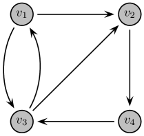
Figure 1: Example of digraph for probabilistic quantized averaging.

Each node $v_{j}\in\mathcal{V}$ follows the Initialization steps ($1-2$) in Algorithm 1, assigning to each of its outgoing edges $v_{l}\in\mathcal{N}_{j}^{+}\cup\{v_{j}\}$ a nonzero probability value $b_{lj}$ equal to $b_{lj}=\frac{1}{1+\mathcal{D}_{j}^{+}}$. The assigned values can be seen in the following matrix

$$\mathcal{B}=\begin{bmatrix}\frac{1}{3}&0&\frac{1}{3}&0\\ \vspace{-0.35cm}\\ \frac{1}{3}&\frac{1}{2}&\frac{1}{3}&0\\ \vspace{-0.35cm}\\ \frac{1}{3}&0&\frac{1}{3}&\frac{1}{2}\\ \vspace{-0.35cm}\\ 0&\frac{1}{2}&0&\frac{1}{2}\\ \vspace{-0.35cm}\\ \end{bmatrix}.$$

Furthermore, each node $v_{j}\in\mathcal{V}$ sets $z_{j}[0]=1$.

For the execution of the proposed algorithm, at time step $k=0$, each node $v_{j}$ calculates its state variables $y^{s}_{j}[0]$, $z^{s}_{j}[0]$ and $q^{s}_{j}[0]$. The mass and state variables for $k=0$ are shown in Table 1. Then, every node $v_{j}$ calculates the values it will transmit. Specifically, nodes $v_{1},v_{2},v_{3},v_{4}$ set $y^{(1)}_{1}[0]=5$, $y^{(1)}_{2}[0]=3$, $y^{(1)}_{3}[0]=7$, $y^{(1)}_{4}[0]=2$ and $z^{(1)}_{1}[0]=1$, $z^{(1)}_{2}[0]=1$, $z^{(1)}_{3}[0]=1$, $z^{(1)}_{4}[0]=1$, respectively. Then, suppose that nodes $v_{1}$, $v_{3}$ and $v_{4}$ transmit to nodes $v_{2}$, $v_{1}$ and $v_{3}$, respectively, whereas node $v_{2}$, performs no transmission (i.e., transmits to itself).

For the execution of the proposed algorithm, each node $v_{j}$ receives from its in-neighbors $v_{i}\in\mathcal{N}_{j}^{-}\cup\{v_{j}\}$ the transmitted mass variables $y_{i}[0]$ and $z_{i}[0]$ and then, at time step $k=1$, it calculates its state variables $y^{s}_{j}[1]$, $z^{s}_{j}[1]$ and $q^{s}_{j}[1]$. The mass and state variables for $k=1$ are shown in Table 1. Here we have that nodes $v_{1}$ and $v_{3}$ have mass variables $y_{1}[1]=y_{3}[0]=7$, $z_{1}[1]=z_{3}[0]=1$ and $y_{3}[1]=y_{4}[0]=2$, $z_{3}[1]=z_{4}[0]=1$ (and update their state variables), while node $v_{2}$ has mass variables $y_{2}[1]=y_{1}[0]+y_{2}[0]=8$, $z_{2}[1]=z_{1}[0]+z_{2}[0]=2$ (also updating its state variables). Then, every node $v_{j}$ calculates the values it will transmit (notice that node $v_{2}$ will split its mass variable $y_{2}[1]$ in two equal pieces since $z_{2}[1]=2$). Specifically, we have that $y^{(1)}_{1}[1]=7$, $y^{(1)}_{2}[1]=4$, $y^{(2)}_{2}[1]=4$, $y^{(1)}_{4}[1]=2$ and $z^{(1)}_{1}[1]=1$, $z^{(1)}_{2}[1]=1$, $z^{(2)}_{2}[1]=1$, $z^{(1)}_{4}[1]=1$, respectively. Then, suppose that nodes $v_{1}$ and $v_{3}$ both transmit to node $v_{2}$, while node $v_{2}$, transmits the set of values $y^{(1)}_{2}[1]$, $z^{(1)}_{2}[1]$ to itself and the set of values $y^{(2)}_{2}[1]$, $z^{(2)}_{2}[1]$ to $v_{4}$.

TABLE I: Initial Mass and State Variables for Fig. 1

Nodes	Mass and State Variables for $k=0$
$v_{j}$	$y_{j}[0]$	$z_{j}[0]$	$y^{s}_{j}[0]$	$z^{s}_{j}[0]$	$q^{s}_{j}[0]$
$v_{1}$	5	1	5	1	5
$v_{2}$	3	1	3	1	3
$v_{3}$	7	1	7	1	7
$v_{4}$	2	1	2	1	2

TABLE II: Mass and State Variables for Fig. 1 for $k=1$

Nodes	Mass and State Variables for $k=1$
$v_{j}$	$y_{j}[1]$	$z_{j}[1]$	$y^{s}_{j}[1]$	$z^{s}_{j}[1]$	$q^{s}_{j}[1]$
$v_{1}$	7	1	7	1	7
$v_{2}$	8	2	8	2	4
$v_{3}$	2	1	2	1	2
$v_{4}$	0	0	2	1	2

Each node $v_{j}$ receives from its in-neighbors the transmitted mass variables and, at time step $k=2$, it calculates its state variables $y^{s}_{j}[2]$, $z^{s}_{j}[2]$ and $q^{s}_{j}[2]$ (which are shown in Table 1). Then, every node $v_{j}$ calculates the values it will transmit as $y^{(1)}_{2}[2]=4$, $y^{(2)}_{2}[2]=4$, $y^{(3)}_{2}[2]=5$, $y^{(1)}_{4}[1]=4$ and $z^{(1)}_{2}[2]=1$, $z^{(2)}_{2}[2]=1$, $z^{(3)}_{2}[2]=1$, $z^{(1)}_{4}[1]=1$, respectively. It is interesting to notice here that all the calculated values $y^{(t)}_{j}[2]$ are equal to the quantized average of the initial values (i.e., the ceiling or the floor of the real average $q=4.25$). Then, suppose that node $v_{4}$ transmits to node $v_{3}$, while node $v_{2}$, transmits the set of values $y^{(1)}_{2}[2]$, $z^{(1)}_{2}[2]$ and $y^{(2)}_{2}[2]$, $z^{(2)}_{2}[2]$ to $v_{4}$ and the set of values $y^{(3)}_{2}[2]$, $z^{(3)}_{2}[2]$ to itself.

TABLE III: Mass and State Variables for Fig. 1 for $k=2$

Nodes	Mass and State Variables for $k=2$
$v_{j}$	$y_{j}[2]$	$z_{j}[2]$	$y^{s}_{j}[2]$	$z^{s}_{j}[2]$	$q^{s}_{j}[2]$
$v_{1}$	0	0	7	1	7
$v_{2}$	13	3	13	3	4
$v_{3}$	0	0	2	1	2
$v_{4}$	4	1	4	1	4

Each node $v_{j}$ receives from its in-neighbors the transmitted mass variables and, at time step $k=3$, it calculates its state variables $y^{s}_{j}[3]$, $z^{s}_{j}[3]$ and $q^{s}_{j}[3]$ (which are shown in Table 1). Then, every node $v_{j}$ calculates the values it will transmit as $y^{(1)}_{2}[3]=5$, $y^{(1)}_{3}[3]=4$, $y^{(1)}_{4}[3]=4$, $y^{(2)}_{4}[3]=4$ and $z^{(1)}_{2}[3]=1$, $z^{(1)}_{3}[3]=1$, $z^{(1)}_{4}[3]=1$, $z^{(2)}_{4}[3]=1$, respectively. Then, suppose that nodes $v_{2}$ and $v_{3}$ transmit to node $v_{1}$ and $v_{4}$, while node $v_{4}$, transmits the set of values $y^{(1)}_{4}[3]$, $z^{(1)}_{4}[3]$ and $y^{(2)}_{4}[3]$, $z^{(2)}_{4}[3]$ to node $v_{3}$.

Next, each node $v_{j}$ receives from its in-neighbors the transmitted mass variables and, at time step $k=4$, it calculates its state variables $y^{s}_{j}[4]$, $z^{s}_{j}[4]$ and $q^{s}_{j}[4]$ which are shown in Table 1.

TABLE IV: Mass and State Variables for Fig. 1 for $k=3$

Nodes	Mass and State Variables for $k=3$
$v_{j}$	$y_{j}[3]$	$z_{j}[3]$	$y^{s}_{j}[3]$	$z^{s}_{j}[3]$	$q^{s}_{j}[3]$
$v_{1}$	0	0	7	1	7
$v_{2}$	5	1	5	1	5
$v_{3}$	4	1	4	1	4
$v_{4}$	8	2	8	2	4

TABLE V: Mass and State Variables for Fig. 1 for $k=4$

Nodes	Mass and State Variables for $k=4$
$v_{j}$	$y_{j}[4]$	$z_{j}[4]$	$y^{s}_{j}[4]$	$z^{s}_{j}[4]$	$q^{s}_{j}[4]$
$v_{1}$	4	1	4	1	4
$v_{2}$	5	1	5	1	5
$v_{3}$	8	2	8	2	4
$v_{4}$	0	0	8	2	4

From Table 1, we can see that for $k\geq 4$ it holds that

$$q_{j}^{s}[k]=\lfloor q\rfloor=4,\ \ \ \text{or}\ \ \ q_{j}^{s}[k]=\lceil q\rceil=5,$$

for every $v_{j}\in\mathcal{V}$, which means that every node $v_{j}$ obtained, after a finite number of iterations, a quantized value $q_{j}^{s}$, which is equal to the ceiling or the floor of the real average $q$ of the initial values of the nodes. The state variable $q_{j}^{s}[k]$ of every node $v_{j}\in\mathcal{V}$ can also be seen in Figure 2, in which we can see that, after a finite number of time steps $k$, it holds that $q_{j}^{s}[k]=4$ or $q_{j}^{s}[k]=5$.

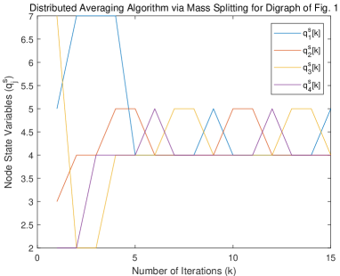
Figure 2: Node state variables plotted against the number of iterations for Algorithm 1 for the digraph shown in Fig. 1.

Remark 3

Notice that the operation of Algorithm 1 is different from the algorithms presented in [29]. Specifically, in [29], the authors presented two distributed algorithms (a probabilistic and a deterministic algorithm) in which every node $v_{j}$ “merged” (i.e., added) the incoming mass variables (which remained “merged” through the algorithm execution), sent by its in-neighbours. The authors showed that every node $v_{j}$ calculated, after a finite number of time steps, a quantized fraction which is equal to the actual average $q$ of the initial values of the nodes (i.e., there was zero quantization error), but due to strict accumulation of the values, the proposed protocol required a significant amount of time steps. During the operation of Algorithm 1, every node $v_{j}$, is able to calculate, after a finite number of steps, a quantized value which is equal to the ceiling or the floor of the initial average (i.e., there is a nonzero quantization error defined as the difference between the actual average $q$ and the quantized average $q^{s}$), but, as we will see in the following sections, its operation outperforms (in terms of convergence speed) the ones presented in [29] along with the state-of-the-art algorithms in the available literature.

V CONVERGENCE OF MASS SPLITTING ALGORITHM

We are now ready to prove that, during the operation of Algorithm 1, each agent $v_{j}$ reaches, after a finite number of time steps, a consensus value which is equal to the ceiling or the floor of the actual average $q$ of the initial values of the nodes. We present the following proposition which is necessary for our subsequent development. Due to space limitations, we do not provide the proof for Proposition 1 below; it will be made available in an extended version of this paper.

Proposition 1

Consider a strongly connected digraph $\mathcal{G}_{d}=(\mathcal{V},\mathcal{E})$ with $n=|\mathcal{V}|$ nodes and $m=|\mathcal{E}|$ edges. Suppose that each node assigns a nonzero probability $b_{lj}$ to each of its outgoing edges $m_{lj}$, where $v_{l}\in\mathcal{N}^{+}_{j}\cup\{v_{j}\}$, as follows

$$b_{lj}=\left\{\begin{array}[]{ll}\frac{1}{1+\mathcal{D}_{j}^{+}},&\mbox{if $l=j$ or $v_{l}\in\mathcal{N}_{j}^{+}$,}\\ 0,&\mbox{if $l\neq j$ and $v_{l}\notin\mathcal{N}_{j}^{+}$,}\end{array}\right.$$

and, at time step $k=0$, node $v_{j}$ holds a “token” while the other nodes $v_{l}\in\mathcal{V}-\{v_{j}\}$ do not. Each node $v_{j}$ transmits the “token” (if it has it, otherwise it performs no transmission) according to the nonzero probability $b_{lj}$ it assigned to its outgoing edges $m_{lj}$. The probability that the token is at node $v_{i}$ after $n-1$ time steps satisfies

$$\text{P}_{\text{Token at node $v_{i}$ at step $n-1$}}\geq(1+D^{+}_{max})^{-(n-1)},$$ (3)

where $D^{+}_{max}=\max_{v_{j}\in\mathcal{V}}D^{+}_{j}$.

Proposition 2

Consider a strongly connected digraph $\mathcal{G}_{d}=(\mathcal{V},\mathcal{E})$ with $n=|\mathcal{V}|$ nodes and $m=|\mathcal{E}|$ edges and $z_{j}[0]=1$ and $y_{j}[0]\in\mathbb{Z}$ for every node $v_{j}\in\mathcal{V}$ at time step $k=0$. Suppose that each node $v_{j}\in\mathcal{V}$ follows the Initialization and Iteration steps as described in Algorithm 1. With probability one, there exists $k_{0}\in\mathbb{Z}_{+}$, so that for every $k\geq k_{0}$ we have

$$q^{s}_{j}[k]=\lceil q\rceil\ \ \text{or}\ \ q^{s}_{j}[k]=\lfloor q\rfloor,$$

for every $v_{j}\in\mathcal{V}$ (i.e., for $k\geq k_{0}$ every node $v_{j}$ has calculated the ceiling or the floor of the actual average $q$ of the initial values).

Proof:

During the Initialization Step $1$ of Algorithm 1, each node $v_{j}\in\mathcal{V}$ assigns a nonzero probability $b_{lj}=\frac{1}{1+\mathcal{D}_{j}^{+}}$ to each of its outgoing edges $m_{lj}$, where $v_{l}\in\mathcal{N}^{+}_{j}\cup\{v_{j}\}$. We can consider the digraph $\mathcal{G}_{d}=(\mathcal{V},\mathcal{E})$ with associated transition matrix $\mathcal{B}=[b_{lj}]$ as a Markov chain in which the nodes of the graph are equivalent to the states of the Markov chain and the weight $b_{lj}$ of matrix $\mathcal{B}$ represents the probability of a transition from node $v_{j}$ towards node $v_{l}$. It is important to notice that during Iteration Steps $1$ and $2$, each node $v_{j}$, splits the received messages $y_{j}[k]$, $z_{j}[k]$ into $z_{j}[k]$ equal (or with maximum difference equal to $1$) pieces $y^{(t)}_{j}[k]$, $z^{(t)}_{j}[k]$, where $y^{(t)}_{j}[k]\in\mathbb{Z}$ and $z^{(t)}_{j}[k]=1$ for $t=1,2,...,z_{j}[k]$. Then it transmits each set of messages $y^{(t)}_{j}[k]$, $z^{(t)}_{j}[k]$ towards a randomly chosen out-neighbour $v_{l}\in\mathcal{N}_{j}^{+}\cup\{v_{j}\}$ according to the nonzero probabilities $b_{lj}$ (assigned during the initialization step). This means that the operation of the Algorithm 1 can be interpreted as the “random walk” of $n$ “tokens” in a Markov chain, where $n=|\mathcal{V}|$, and each ‘token contains a set of values $y[k]$, $z[k]$, for which $y[k]\in\mathbb{Z}$ and $z[k]=1$, during each time step $k$.

During the operation of Algorithm 1, from Iteration Step $1$, we have that if two “tokens” meet in the same node (say $v_{j}$), during time step $k$, then their values $y[k]$ become equal (or with maximum difference equal to $1$). Furthermore, the sum of the $y_{j}[k]$ values at any given $k$ is equal to the initial sum (i.e., $\sum_{j=1}^{n}y_{j}[k]=\sum_{j=1}^{n}y_{j}[0]$). Thus, we will focus on the scenario in which all $n$ tokens meet at a common node and obtain equal values $y[k]$ (or with maximum difference between them equal to $1$).

From Proposition 1, we have that after $n-1$ time steps, the probability that one “token” is at node $v_{i}$ is

$$\text{P}_{\text{Token at node $v_{i}$ at step $n-1$}}\geq(1+D^{+}_{max})^{-(n-1)}.$$

Considering that, during the operation of Algorithm 1, the $n$ “tokens” perform independent random walks we have that the probability that all $n$ tokens meet at node $v_{i}$ after $n-1$ time steps is

$$\text{P}_{\text{All tokens at node $v_{i}$ at step $n-1$}}\geq(1+D^{+}_{max})^{-n(n-1)}.$$

Furthermore, since the events “all tokens meet at node $v_{i}$ after $n-1$ time steps” and “all tokens meet at node $v_{j}$ after $n-1$ time steps” are mutually exclusive (i.e., they have a zero intersection) then we have that the probability that all tokens meet at any node $v_{j}\in\mathcal{V}$ after $n-1$ time steps is

$$\text{P}_{\text{All tok. at node $v_{i}$ at step $n-1$}} \geq \sum_{v_{j}\in\mathcal{V}}(1+D^{+}_{max})^{-n(n-1)}\Rightarrow$$

$$\text{P}_{\text{All tok. at node $v_{i}$ at step $n-1$}} \geq n(1+D^{+}_{max})^{-n(n-1)}.\;$$

This means that, for the scenario “not all tokens meet at any node after $n-1$ time steps” we have

$$\text{P}_{\text{Not all tok. at any node at step $n-1$}}\leq 1-n(1+D^{+}_{max})^{-n(n-1)}.$$ (4)

Note that $\text{P}_{\text{Not all tok. at any node at step $n-1$}}$ denotes the probability that no node will receive all $n$ tokens after $n-1$ time steps.

By extending the above analysis we have that after $\tau(n-1)$ time steps (i.e., $\tau$ windows, each one consisting of $n-1$ time steps), we have that the probability that “not all tokens meet at any node after $\tau$ time steps” is

$$\text{P}_{\text{Not all tok. at any node after $\tau$}}\leq[\text{P}_{\text{Not all tok. at any node at step $n-1$}}]^{\tau}.$$ (5)

Since, from (4), we have that $P_{not\ all}<1$ this means that, by executing Algorithm 1 for $\tau$ time windows, from (5) we have that

$$\lim_{\tau\rightarrow\infty}\text{P}_{\text{Not all tok. at any node after $\tau$}}=0.$$ (6)

As a result, with probability $1$, we have that $\exists k_{0}^{\prime}\in\mathbb{Z}$ for which all $n$ “tokens” meet at node $v_{j}$. This means that all $n$ “tokens” will have equal values $y[k_{0}^{\prime}]$ (or with maximum differences between them equal to $1$). Furthermore, from Iteration Step $1$, we have that each node $v_{j}$ splits $y_{j}[k]$ in $z_{j}[k]$ equal (or with maximum difference between them equal to $1$) pieces $y^{(t)}_{j}[k]$, $z^{(t)}_{j}[k]$, where $y^{(t)}_{j}[k]\in\mathbb{Z}$ and $z^{(t)}_{j}[k]=1$ for $t=1,2,...,z_{j}[k]$ for which it holds that $\sum_{t=1}^{z_{j}[k]}y^{(t)}_{j}[k]=y_{j}[k]$ and $\sum_{t=1}^{z_{j}[k]}z^{(t)}_{j}[k]=z_{j}[k]$. This means that $\sum_{j=1}^{n}y[k_{0}^{\prime}]=\sum_{j=1}^{n}y[0]$ and we have that the $y[k_{0}^{\prime}]$ values of each “token” will become equal to the ceiling or the floor of the actual average $q$ of the initial values (i.e., $y[k_{0}^{\prime}]=\lfloor q\rfloor$ or $y[k_{0}^{\prime}]=\lceil q\rceil$).

Continuing the operation of Algorithm 1, we have that, for time steps $k>k_{0}^{\prime}$, the $n$ “tokens” will continue performing random walks in the digraph $\mathcal{G}_{d}$. This means that, since $\mathcal{G}_{d}$ is strongly connected, we have that $\exists k_{0}\in\mathbb{N}$, where $k_{0}>k_{0}^{\prime}$, for which every node $v_{j}\in\mathcal{V}$ will receive (at least once) one (or multiple) “tokens” during the time interval $(k_{0}^{\prime},k_{0}]$. From Iteration Step $1$, this means that the state variables $q_{j}[k_{0}]$ of every node $v_{j}\in\mathcal{V}$, will be equal to the ceiling or the floor of the actual average $q$ (i.e., $q_{j}[k_{0}]=\lceil q\rceil$ or $q_{j}[k_{0}]=\lfloor q\rfloor$, for every $v_{j}\in\mathcal{V}$) which completes the proof of this proposition. ∎

VI SIMULATION RESULTS

In this section, we present simulation results and comparisons. Specifically, we present simulation results of the proposed distributed algorithm for the digraph $\mathcal{G}_{d}=(\mathcal{V},\mathcal{E})$ (borrowed from [31]), shown in Fig. 3, with $\mathcal{V}=\{v_{1},v_{2},v_{3},v_{4},v_{5},v_{6},v_{7}\}$ and $\mathcal{E}=\{m_{21},m_{51},m_{12},m_{52},m_{13},m_{53},m_{24},m_{54},m_{65},m_{75},$ $m_{36},m_{47},m_{67}\}$, where each node has initial quantized values $y_{1}[0]=15$, $y_{2}[0]=5$, $y_{3}[0]=11$, $y_{4}[0]=4$, $y_{5}[0]=3$, $y_{6}[0]=13$, and $y_{7}[0]=9$, respectively. The real average $q$ of the initial values of the nodes, is equal to $q=\frac{57}{7}=8.57$ which means that the quantized average $q^{s}$ is equal to $q^{s}=8$ or $q^{s}=9$.

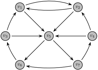
Figure 3: Example of digraph for simulation of Algorithm 1.

In Figure 4 we plot the state variable $q_{j}^{s}[k]$ of every node $v_{j}\in\mathcal{V}$ as a function of the number of iterations $k$ for the digraph shown in Fig. 3. The plot demonstrates that Algorithm 1 is able to achieve a common quantized consensus value to the average of the initial states after a finite number of iterations.

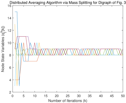
Figure 4: Node state variables plotted against the number of iterations for Algorithm 1 for the digraph shown in Fig. 3.

Now, we compare its performance against four other algorithms: (a) the quantized gossip algorithm presented in [15] in which, at each time step $k$, one edge is selected at random, independently from earlier instants and the values of the nodes that the selected edge is incident on are updated, (b) the quantized asymmetric averaging algorithm presented in [18] in which, at each time step $k$, one edge, say edge $(v_{l},v_{j})$, is selected at random and, node $v_{j}$ sends its state information and surplus and node $v_{l}$ performs updates over its own state and surplus values, (c) the distributed averaging algorithm with quantized communication presented in [17] in which, at each time step $k$, each agent $v_{j}$ broadcasts a quantized version of its own state value towards its out-neighbors, (d) the distributed averaging algorithm with quantized communication presented in [29] in which, at each time step $k$, each agent sends its mass variables towards a randomly chosen out-neighbor in the form of a quantized fraction.

Figure 5 presents a study of the case of $1000$ digraphs of $20$ nodes each, in which the average of the nodes initial values is equal to $q=\dfrac{651}{20}=32.55$. The results shown are averaged over $1000$ graphs. The top of Figure 5 suggests that the operation of Algorithm 1 outperforms the quantized distributed algorithms in the available literature [15, 18, 17, 29].

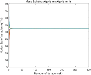
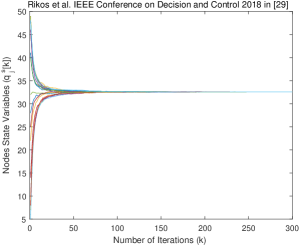
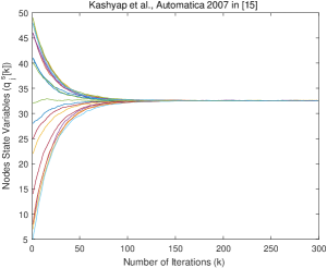
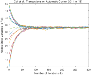
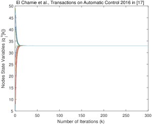
Figure 5: Comparison between Algorithm 1, the distributed averaging algorithm with quantized communication in [29], the quantized gossip algorithm presented in [15], the quantized asymmetric averaging algorithm presented in [18], and the distributed averaging algorithm with quantized communication presented in [17] for $1000$ random averaged digraphs of $20$ nodes each.

Remark 4

It is worth noting, that the quantized distributed algorithms in [15, 18] only involve a single exchange between a single randomly chosen pair of neighboring nodes at each iteration. Furthermore, the doubly stochastic matrix which is necessary for the operation of the distributed algorithm in [17] was formulated by (i) calculating a set of edge weights that balance the given strongly connected digraph with the distributed strategies presented in [31] and (ii) by performing a max consensus protocol, adding a nonzero self-loop for every node $v_{j}$, and normalizing, according to the distributed strategies presented in [32].

VII CONCLUSIONS

We have considered the quantized average consensus problem and presented a randomized distributed averaging algorithm in which the processing, storing and exchange of information between neighboring agents is subject to uniform quantization. We analyzed its operation, established that it will reach quantized consensus after a finite number of iterations and argued that its convergence speed appears to be the fastest in the available literature, which allows convergence to the quantized average of the initial values after a finite number of time steps, without any specific requirements regarding the network that describes the underlying communication topology (see [17]).

In the future we plan to extend the operation of the proposed algorithm to more realistic cases, such as transmission delays over the communication links and the presence of unreliable links over the communication network. Furthermore, we plan to design distributed strategies under which every agent in the network will be able to determine whether quantized average consensus has been reached (and thus proceed to execute more complicated control or coordination tasks).

References

- [1] L. Xiao, S. Boyd, and S. Lall, “A scheme for robust distributed sensor fusion based on average consensus,” Proceedings of the International Symposium on Information Processing in Sensor Networks, pp. 63–70, April 2005.
- [2] R. Olfati-Saber and R. Murray, “Consensus problems in networks of agents with switching topology and time-delays,” IEEE Transactions on Automatic Control, vol. 49, no. 9, pp. 1520–1533, September 2004.
- [3] N. Lynch, Distributed Algorithms. San Mateo: CA: Morgan Kaufmann Publishers, 1996.
- [4] V. D. Blondel, J. M. Hendrickx, A. Olshevsky, and J. N. Tsitsiklis, “Convergence in multiagent coordination, consensus, and flocking,” Proceedings of the IEEE Conference on Decision and Control, pp. 2996–3000, 2005.
- [5] L. Schenato and G. Gamba, “A distributed consensus protocol for clock synchronization in wireless sensor network,” Proceedings of the IEEE Conference on Decision and Control, pp. 2289–2294, 2007.
- [6] C. N. Hadjicostis, A. D. Domínguez-García, and T. Charalambous, “Distributed averaging and balancing in network systems, with applications to coordination and control,” Foundations and Trends® in Systems and Control, vol. 5, no. 3–4, 2018.
- [7] S. Sundaram and C. N. Hadjicostis, “Distributed function calculation and consensus using linear iterative strategies,” IEEE Journal on Selected Areas in Communications, vol. 26, no. 4, pp. 650–660, May 2008.
- [8] T. Charalambous, Y. Yuan, T. Yang, W. Pan, C. N. Hadjicostis, and M. Johansson, “Decentralised minimum-time average consensus in digraphs,” Proceedings of the IEEE Conference on Decision and Control (CDC), pp. 2617–2622, 2013.
- [9] L. Xiao and S. Boyd, “Fast linear iterations for distributed averaging,” Systems and Control Letters, vol. 53, no. 1, pp. 65–78, September 2004.
- [10] A. G. Dimakis, S. Kar, J. M. F. Moura, M. G. Rabbat, and A. Scaglione, “Gossip algorithms for distributed signal processing,” Proceedings of the IEEE, vol. 98, no. 11, pp. 1847–1864, November 2010.
- [11] J. Liu, S. Mou, A. S. Morse, B. D. O. Anderson, and C. Yu, “Deterministic gossiping,” Proceedings of the IEEE, vol. 99, no. 9, pp. 1505–1524, September 2011.
- [12] J. Tsitsiklis, “Problems in decentralized decision making and computation,” Ph.D. dissertation, Massachusetts Institute of Technology, Cambridge, MA, Cambridge, 1984.
- [13] T. C. Aysal, M. Coates, and M. Rabbat, “Distributed average consensus using probabilistic quantization,” IEEE/SP Workshop on Statistical Signal Processing, pp. 640–644, 2007.
- [14] J. Lavaei and R. M. Murray, “Quantized consensus by means of gossip algorithm,” IEEE Transactions on Automatic Control, vol. 57, no. 1, pp. 19–32, January 2012.
- [15] A. Kashyap, T. Basar, and R. Srikant, “Quantized consensus,” Automatica, vol. 43, no. 7, pp. 1192–1203, 2007.
- [16] R. Carli, F. Fagnani, A. Speranzon, and S. Zampieri, “Communication constraints in the average consensus problem,” Automatica, vol. 44, no. 3, pp. 671–684, 2008.
- [17] M. E. Chamie, J. Liu, and T. Basar, “Design and analysis of distributed averaging with quantized communication,” IEEE Transactions on Automatic Control, vol. 61, no. 12, pp. 3870–3884, December 2016.
- [18] K. Cai and H. Ishii, “Quantized consensus and averaging on gossip digraphs,” IEEE Transactions on Automatic Control, vol. 56, no. 9, pp. 2087–2100, September 2011.
- [19] G. S. Seyboth, D. V. Dimarogonas, and K. H. Johansson, “Event-based broadcasting for multi-agent average consensus,” Automatica, vol. 49, no. 1, pp. 245–252, January 2013.
- [20] C. Nowzari and J. Cortés, “Distributed event-triggered coordination for average consensus on weight-balanced digraphs,” Automatica, vol. 68, pp. 237–244, June 2016.
- [21] Z. Liu, Z. Chen, and Z. Yuan, “Event-triggered average-consensus of multi-agent systems with weighted and direct topology,” Journal of Systems Science and Complexity, vol. 25, no. 5, pp. 845–855, October 2012.
- [22] A. Nedic, A. Olshevsky, A. Ozdaglar, and J. Tsitsiklis, “On distributed averaging algorithms and quantization effects,” IEEE Transactions on Automatic Control, vol. 54, no. 11, pp. 2506–2517, November 2009.
- [23] S. Kar and J. M. F. Moura, “Distributed consensus algorithms in sensor networks: Quantized data and random link failures,” IEEE Transactions on Signal Processing, vol. 58, no. 3, pp. 1383–1400, March 2010.
- [24] F. Benezit, P. Thiran, and M. Vetterli, “The distributed multiple voting problem,” IEEE Journal of Selected Topics in Signal Processing, vol. 5, no. 4, pp. 791–804, August 2011.
- [25] T. Li, M. Fu, L. Xie, and J. F. Zhang, “Distributed consensus with limited communication data rate,” IEEE Transactions on Automatic Control, vol. 56, no. 2, pp. 279–292, February 2011.
- [26] D. Thanou, E. Kokiopoulou, Y. Pu, and P. Frossard, “Distributed average consensus with quantization refinement,” IEEE Transactions on Signal Processes, vol. 61, no. 1, pp. 194–295, January 2013.
- [27] S. Etesami and T. Basar, “Convergence time for unbiased quantized consensus over static and dynamic networks,” IEEE Transactions on Automatic Control, vol. 61, no. 2, pp. 443–455, February 2016.
- [28] T. Basar, S. Etesami, and A. Olshevsky, “Fast convergence of quantized consensus using metropolis chains,” Proceedings of the IEEE Conference on Decision and Control, pp. 1330–1334, December 2014.
- [29] A. I. Rikos and C. N. Hadjicostis, “Distributed average consensus under quantized communication via event-triggered mass summation,” Proceedings of the IEEE Conference on Decision and Control (CDC), pp. 894–899, 2018.
- [30] B. Gharesifard and J. Cortés, “Distributed strategies for making a digraph weight-balanced,” Proceedings of the Annual Allerton Conference on Communication, Control, and Computing, pp. 771–777, 2009.
- [31] A. I. Rikos, T. Charalambous, and C. N. Hadjicostis, “Distributed weight balancing over digraphs,” IEEE Transactions on Control of Network Systems, vol. 1, no. 2, pp. 190–201, June 2014.
- [32] B. Gharesifard and J. Cortés, “Distributed strategies for generating weight-balanced and doubly stochastic digraphs,” European Journal of Control, vol. 18, no. 6, pp. 539–557, 2012.