Time delays in ultracold atomic and molecular collisions

Abstract

We study the behavior of the Eisenbud-Wigner collisional time delay around Feshbach resonances in cold and ultracold atomic and molecular collisions. We carry out coupled-channels scattering calculations on ultracold Rb and Cs collisions. In the low-energy limit, the time delay is proportional to the scattering length, so exhibits a pole as a function of applied field. At high energy, it exhibits a Lorentzian peak as a function of either energy or field. For narrow resonances, the crossover between these two regimes occurs at an energy proportional to the square of the resonance strength parameter $s_{\textrm{res}}$. For wider resonances, the behavior is more complicated and we present an analysis in terms of multichannel quantum defect theory.

I Introduction

Scattering resonances are important in many fields, from nuclear physics to physical chemistry. A resonance occurs when a collision occurs at an energy close to that of a quasibound state of the collision complex, so that scattering flux is temporarily trapped at short range. Resonant scattering is different in character from non-resonant scattering, and often produces different products and characteristic angular distributions; it typically produces strong features in the dependence of collision properties on energy and external fields. There are particularly important applications in ultracold atomic physics, where magnetically tunable Feshbach resonances are used to control the behavior of ultracold atoms.

The language of resonant scattering is often used to understand physical phenomena. A quasibound state has a width that depends on its coupling to energetically open channels, and the width is interpreted as inversely proportional to the lifetime of the state. Conversely, resonant collisions experience a resonant time delay, which is also usually supposed to be inversely proportional to the resonance width. However, as will be seen below, this simple viewpoint breaks down in the low-energy regime close to threshold.

A topical application of resonant time delays, which motivated the current study, is in collisions of ultracold molecules. If the interaction potential for a colliding pair has a deep well, the collision complex can have a high density of states even at low collision energies Mayle et al. (2012, 2013); Christianen et al. (2019a). The resulting dense pattern of scattering resonances may produce long-lived “sticky” collisions in the ultracold regime. The collision complexes may be destroyed either by collision with a third body Mayle et al. (2013) or by laser-driven processes Christianen et al. (2019b). If the lifetime of the complex is long compared to the destruction mechanism, the overall process displays second-order kinetics. Multiple experiments have reported short trap lifetimes for molecules that have no 2-body collisional loss mechanism Takekoshi et al. (2014); Molony et al. (2014); Park et al. (2015); Guo et al. (2016); Ye et al. (2018), which may be a sign of such effects. Gregory et al. Gregory et al. (2019) have demonstrated that the kinetics of the loss process are indeed second order for ultracold RbCs. It is thus important to understand collisional time delays in the ultracold regime.

The theory of collisional time delays in quantum scattering was established by Eisenbud, Eisenbud (1948), Wigner Wigner (1955) and Smith Smith (1960). It has been used to analyse resonant contributions to recombination at non-ultracold temperatures Kendrick and T Pack (1995, 1996). In a few cases time delays have been calculated for ultracold scattering Field and Madsen (2003); Guillon and Stoecklin (2009); Bovino et al. (2011); Simoni et al. (2009); Croft et al. (2017); Mehta et al. (2018). However, there has been little work on understanding the basic properties and behaviors of the time delay in ultracold collisions. The purpose of the present paper is to explore how time delays behave close to threshold. We will show that, in this regime, the time delay does not show a simple peak around a resonance. The behavior is particularly striking when viewed as a function of external field rather than energy: as a function of field, the time delay may be either positive or negative, and in the low-energy limit averages to zero across a resonance. We will illustrate the behavior with calculations on resonances in ultracold atomic collisions, and discuss the transition from the threshold regime to higher energy.

II Eisenbud-Wigner-Smith Time Delay

Eisenbud Eisenbud (1948) and Wigner Wigner (1955) used a wavepacket analysis to define a time delay for single-channel scattering,

$$Q(E)=2\hbar\frac{d\delta}{dE},$$ (1)

where $\delta$ is the scattering phase shift and $E$ is the energy. Smith Smith (1960) considered the problem in a time-independent formalism and defined a time-delay matrix suitable for multichannel scattering,

$$\boldsymbol{Q}(E)=i\hbar\boldsymbol{S}\frac{d\boldsymbol{S}^{\dagger}}{dE},$$ (2)

in terms of the scattering matrix $\boldsymbol{S}$. If there is only a single open channel, $\boldsymbol{S}=e^{2{\rm i}\delta}$ and Eq. (2) reduces to Eq. (1). The present work will focus on the case of a single open channel, but will consider Feshbach resonances due to the effects of additional closed channels.

II.1 Far above threshold

We first consider an isolated narrow resonance far above threshold. The elastic scattering phase shift follows a Breit-Wigner form as a function of energy at constant field,

$$\delta(E)=\delta_{\rm bg}(E)+\arctan\left[\frac{\frac{1}{2}\Gamma_{\textrm{E}}(E)}{E_{\textrm{res}}-E}\right],$$ (3)

where $\delta_{\rm bg}(E)$ is a background phase shift that is a slow function of energy, $E_{\textrm{res}}$ is the resonance energy, and $\Gamma_{\textrm{E}}(E)$ is the resonance width in energy. The phase shift increases by $\pi$ above its background value across the width of a resonance. Far above threshold, the dependence of $\Gamma_{\textrm{E}}$ on $E$ can usually be neglected, and the time delay is Smith (1960)

$$Q(E)=Q_{\rm bg}(E)+\frac{\hbar\Gamma_{\textrm{E}}}{(E_{\textrm{res}}-E)^{2}+\Gamma_{\textrm{E}}^{2}/4}.$$ (4)

This shows a simple Lorentzian peak as a function of energy. Neglecting the background term, the integral across this peak is $2\pi\hbar$, independent of $\Gamma_{\textrm{E}}$. An important consequence of this is that, if $\Gamma_{\textrm{E}}(E)\ll k_{\rm B}T$, the resonant contribution to a thermally averaged time delay is independent of the width of the resonance. Thus, under some circumstances, the contribution of a large number of narrow resonances can be understood from the density of states without any more detailed understanding of the interactions and dynamics. An approximation of this form was used by Bowman Bowman (1986) to obtain an alternative derivation of RRKM theory.

For cold collisions it is common to consider the resonance as a function of external field (here taken to be magnetic field $B$), at a constant collision energy $E$ with respect to a (potentially field-dependent) threshold energy $E_{\textrm{thresh}}$. The phase shift is given by

$$\delta(E,B)=\delta_{\textrm{bg}}(E)+\arctan\left[\frac{\frac{1}{2}\Gamma_{\textrm{B}}(E)}{B-B_{\textrm{res}}^{\textrm{BW}}(E)}\right].$$ (5)

Here $B_{\textrm{res}}^{\textrm{BW}}(E)$ is the position of resonance in field. Far from threshold $B_{\textrm{res}}^{\textrm{BW}}(E)$ varies with energy according to the magnetic moment of the resonant state relative to the threshold, $\mu_{\textrm{rel}}=d(E_{\textrm{bound}}-E_{\textrm{thresh}})/dB$. The resonance width in field is $\Gamma_{\textrm{B}}(E)=\Gamma_{\textrm{E}}(E)/\mu_{\textrm{rel}}$. The time delay can then be written

$$Q(E,B)=Q_{\rm bg}(E)+\frac{\hbar\Gamma_{\textrm{B}}(E)/\mu_{\textrm{rel}}}{[B_{\textrm{res}}^{\textrm{BW}}(E)-B]^{2}+\Gamma_{\textrm{B}}(E)^{2}/4}.$$ (6)

Far above threshold, the time delay thus shows a Lorentzian peak as a function of external field as well as energy.

II.2 Ultracold scattering

In the ultracold regime, scattering is modified by threshold effects Wigner (1948). These are conveniently expressed in terms of the wavenumber $k$, where $E=\hbar^{2}k^{2}/2\mu$ and $\mu$ is the collisional reduced mass. A key quantity is the $k$-dependent scattering length,

$$a(k,B)=\frac{-\tan\delta(k,B)}{k}.$$ (7)

For some purposes it is sufficient to consider only the zero-energy scattering length, $a(B)=\lim_{k\to 0}a(k,B)$; in the low-energy limit, $\delta=-ka(B)$, and Field and Madsen (2003)

$$Q=\frac{-2a(B)\mu}{\hbar k}=-2\frac{a(B)}{v}$$ (8)

where $v=k\hbar/\mu$ is the collision velocity. This is exactly the classical time delay associated with a hard-sphere collision with radius $a(B)$ Simoni et al. (2009), in accordance with the usual interpretation of the scattering length.

Around a low-energy Feshbach resonance, the scattering length shows a pole as a function of field Moerdijk et al. (1995),

$$a(k,B)=a_{\textrm{bg}}(k)\left[1-\frac{\Delta(E)}{B-B_{\textrm{res}}^{\textrm{pole}}(E)}\right],$$ (9)

where $\Delta(E)$ characterizes the width of the pole. The pole position $B_{\textrm{res}}^{\textrm{pole}}(E)$ coincides with $B_{\textrm{res}}^{\textrm{BW}}(E)$ at zero energy, but they generally differ away from threshold, as discussed in section IV. As the scattering length passes through both large positive and large negative values near the pole, Eq. (8) implies that there are both positive and negative time delays around a resonance in the low-energy limit van Dijk and Kiers (1992); Field and Madsen (2003). This behavior is very different from that seen away from threshold, Eq. (4), where the resonant contribution to the time delay is strictly positive.

II.3 Intermediate regime

In order to reconcile the different behavior of $Q$ close to threshold and far from it, it is necessary to consider the energy dependence of the resonance parameters. The phase shift can still be written in the form (5), but the derivatives of the parameters with respect to energy are important. The full expression for the time delay is

$$Q(E,B) =Q_{\textrm{bg}}(E)$$

$$+\frac{d\Gamma_{\textrm{B}}}{dE}\frac{\hbar[B-B_{\textrm{res}}^{\textrm{BW}}(E)]}{[B-B_{\textrm{res}}^{\textrm{BW}}(E)]^{2}+\Gamma_{\textrm{B}}(E)^{2}/4}$$

$$+\frac{dB_{\textrm{res}}^{\textrm{BW}}}{dE}\frac{\hbar\Gamma_{\textrm{B}}(E)}{[B-B_{\textrm{res}}^{\textrm{BW}}(E)]^{2}+\Gamma_{\textrm{B}}(E)^{2}/4}.$$ (10)

In the high-energy limit, $d\Gamma_{\textrm{B}}/dE=0$ and Eq. (10) reduces to Eq. (6). In the low-energy limit, the energy dependence of the width can be written $\Gamma_{\textrm{B}}(E)=2ka_{\textrm{bg}}\Delta$ Mies et al. (2000); $d\Gamma_{\textrm{B}}/dE$ diverges as $k\rightarrow 0$, so the second term in Eq. (10) dominates.

The crossover between these limiting behaviors occurs around a crossover energy $E_{\textrm{X}}$ where the two derivatives in Eq. (10) are equal. As described below, the threshold has little effect on $B_{\textrm{res}}^{\textrm{BW}}(E)$ when the resonance is narrow or $a_{\textrm{bg}}$ is close to $\bar{a}$, where $\bar{a}=0.4779888\dots\times(2\mu C_{6}/\hbar^{2})^{1/4}$ is the mean scattering length of Gribakin and Flambaum Gribakin and Flambaum (1993) for an interaction potential $-C_{6}R^{-6}$. $dB_{\textrm{res}}^{\textrm{BW}}/dE$ is thus approximately $1/\mu_{\textrm{rel}}$, and the low-energy expression for $\Gamma_{\textrm{B}}(E)$ gives

$$E_{\textrm{X}}\approx\frac{2\mu}{\hbar^{2}}a_{\textrm{bg}}^{2}\Delta^{2}\mu_{\textrm{rel}}^{2}=s_{\textrm{res}}^{2}\bar{E}.$$ (11)

Here, the dimensionless resonance strength parameter Chin et al. (2010) is $s_{\textrm{res}}=a_{\textrm{bg}}\Delta\mu_{\textrm{rel}}/(\bar{a}\bar{E})$, where $\bar{E}=\hbar^{2}/2\mu\bar{a}^{2}$. Substituting back into Eq. (10), at $E=E_{\textrm{X}}$ we expect the peak in $Q$ to be about 20 times larger than the trough for a narrow resonance.

III Numerical examples

Table 1: Parameters for the example resonances, obtained from coupled-channels calculations.

Res.	Isotope	$\bar{a}/a_{0}$	$\bar{E}/k_{\textrm{B}}$ ($\mu$K)	$B_{\textrm{res}}^{\textrm{pole}}(0)$ (G)	$a_{\textrm{bg}}/a_{0}$	$\Delta$ (G)	$\mu_{\textrm{rel}}/\mu_{\textrm{B}}$	$s_{\textrm{res}}$	$E_{\textrm{X}}/k_{\textrm{B}}$ ($\mu$K)	$\bar{\Gamma}_{\textrm{B}}$ (mG)
1	87Rb	79.0	319	1007.86	100	0.20	2.8	0.15	7.2	476
2	87Rb	79.0	319	686.60	100	0.0072	1.3	0.0025	0.0020	17
3	133Cs	96.6	140	47.79	1008	0.15	1.2	0.88	110	35
4	85Rb	78.5	331	851.3	$-390$	$-1.2$	2.1	2.6	2200	324

We illustrate the behavior with calculations on resonances in collisions of Rb and Cs atoms. We carry out coupled-channels calculations to evaluate energy-dependent phase shifts in magnetic fields using the molscat Hutson and Le Sueur (2019a, b) package. The methods used are similar to those described in Ref. Blackley et al., 2013. We use the interaction potentials of Strauss et al. Strauss et al. (2010) for Rb and Berninger et al. Berninger et al. (2013) for Cs. The energy derivatives required for the time delay are calculated by finite difference from two calculations at energies that differ by 0.1%.

We take four resonances in ultracold Rb and Cs scattering as examples: (1) The resonance near 1007 G for ⁸⁷Rb Marte et al. (2002); Volz et al. (2003); Dürr et al. (2004); (2) the resonance near 687 G for ⁸⁷Rb Marte et al. (2002); Dürr et al. (2004); (3) the resonance near 47 G for ¹³³Cs Chin et al. (2004); Lange et al. (2009); and (4) the resonance near 850 G for ⁸⁵Rb Blackley et al. (2013). All these resonances are for atoms in their lowest hyperfine and Zeeman state, so we do not need to consider effects of inelastic scattering. Scattering involving non-s-wave open channels is negligible, so we consider only one open channel and use Eq. (1). For each resonance we find $B^{\textrm{pole}}_{\textrm{res}}(0)$, $a_{\textrm{bg}}$, and $\Delta$ from coupled-channels calculations by converging on and characterizing the pole in scattering length using the methods of Frye and Hutson Frye and Hutson (2017). To obtain $\mu_{\textrm{rel}}$, we carry out coupled-channels calculations of the energy of the bound state in a near-linear region below threshold, using the bound package Hutson and Le Sueur (2019c, b). Table 1 lists these parameters, together with other relevant quantities including $s_{\textrm{res}}$ and $E_{\textrm{X}}$, for each of the resonances. Resonance 1 is the widest known for ground-state ⁸⁷Rb, but is of only moderate width compared to resonances in other similar systems; its background scattering length is close to $\bar{a}_{\textrm{87Rb}}$. Resonance 2 is significantly narrower and has essentially the same background scattering length. Resonance 3 has a similar width $\Delta$ to resonance 1, but a much larger background scattering length, $a_{\textrm{bg}}\approx 10\bar{a}_{\textrm{133Cs}}$, so that $s_{\textrm{res}}$ is significantly larger. Resonance 4 is a broad resonance with a large negative scattering length, $a_{\textrm{bg}}\approx-5\bar{a}_{\textrm{85Rb}}$.

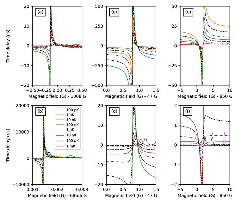
Figure 1: Time delay $Q$ as a function of magnetic field $B$ at various energies for the four example resonances. Dashed and dotted lines show energies 2 and 5 times those of the corresponding solid lines. (a) resonance 1; (b) resonance 2; (c) and (d) resonance 3; (e) and (f) resonance 4.

Figure 1 shows the time delay for the example resonances as a function of magnetic field for a variety of energies from 100 pK up to 1 mK. Figure 1(a) shows the time delay for resonance 1, for which $E_{\textrm{X}}/k_{\textrm{B}}=7.2$ $\mu$K. At the lowest energy shown, 100 nK, it has a large symmetrical pole-like oscillation and deviates from this only in a small region near the center. The difference in behavior between the lowest few energies in the wings of the resonance is mostly due to the dependence on $k$ in Eq. (8). The pole-like behavior is suppressed in a region near the center due to the denominator in the second term of Eq. (10); the width of this region is proportional to $\Gamma_{\textrm{B}}(E)$, so it broadens as the energy increases, greatly reducing the magnitude of the peak and trough. The importance of the second term of Eq. (10) decreases with increasing energy; by 1 $\mu$K the oscillation is significantly asymmetric, and by 10 $\mu$K the trough has disappeared entirely, leaving a single peak that starts to shift away from the zero-energy resonance position. This agrees well with the crossover energy $E_{\textrm{X}}/k_{\textrm{B}}=7.2$ $\mu$K predicted by Eq. (11). The peak then continues to move off to high field and broaden towards its high-energy form.

Figure 1(b) shows the behavior around resonance 2, for which $E_{\textrm{X}}/k_{\textrm{B}}=2$ nK. It shows similar features to resonance 1, but they occur at much lower energy. The oscillation is already highly asymmetric at 1 nK. By 10 nK the trough has disappeared and $Q$ reaches its high-energy form well below 100 nK.

Figures 1(c) and (d) show the behavior around resonance 3. As for resonances 1 and 2, the oscillation is pole-like and symmetric at the lowest energies, but it develops significant asymmetry by 100 nK, which is far below the crossover energy predicted by Eq. (11), $E_{\textrm{X}}/k_{\textrm{B}}\approx 110\ \mu$K. The shape of $Q$ has become a single peak by 1 $\mu$K. Above 5 $\mu$K the peak shifts to higher field and gets narrower and higher.

Figures 1(e) and (f) show the behavior around resonance 4. In this case, the transition from low-energy to high-energy behavior is more complicated. The oscillation becomes asymmetric around 1 $\mu$K and it is the trough that is initially more pronounced than the peak. As for resonance 3, this happens well below the crossover energy predicted by Eq. (11), $E_{\textrm{X}}/k_{\textrm{B}}\approx 2.2$ mK. By 10 $\mu$K, $Q$ has just a single trough with no visible peak, but by 100 $\mu$K this has inverted to a single peak with no trough. Above 100 $\mu$K, the peak shifts away to higher field and, as for resonance 3, gets narrower and higher.

The behavior of the time delay for resonances 1 and 2 follows the simple theory described in section 2. However, the approximate forms of the resonance parameters used in deriving Eq. (11) are not valid for a broad resonance with $a_{\textrm{bg}}$ far from $\bar{a}$. Understanding the more complicated behavior for resonances 3 and 4 show needs a more complete description of the threshold effects. This is given in the following section.

IV Interpretation using multichannel quantum defect theory

Multichannel quantum-defect theory (MQDT) provides a unified framework for describing scattering both close to and far from threshold. We use a 2-channel MQDT model of the resonance in the formalism of Mies and Raoult Mies and Raoult (2000), as described in detail by Jachymski and Julienne Jachymski and Julienne (2013). This model accurately reproduce the coupled-channels results. In the model, the width and position of a resonance can be written as

$$\Gamma_{\textrm{B}}(E) =\bar{\Gamma}_{\textrm{B}}C^{-2}(E)$$ (12)

$$B_{\textrm{res}}^{\textrm{BW}}(E) =B_{0}+\frac{E}{\mu_{\textrm{rel}}}-\frac{1}{2}\bar{\Gamma}_{\textrm{B}}\tan\lambda(E).$$ (13)

Here, $\bar{\Gamma}_{\textrm{B}}$ is the short-range width in field, neglecting threshold effects, which is independent of both $E$ and $B$, and $B_{0}$ is the field at which the bare (uncoupled) bound state crosses threshold. They are related to $\Delta$ and $B_{\textrm{res}}^{\textrm{pole}}(0)$ by Julienne and Gao (2006)

$$\frac{1}{2}\bar{\Gamma}_{\textrm{B}} =\frac{r_{\textrm{bg}}}{1+(1-r_{\textrm{bg}})^{2}}\Delta$$ (14)

$$B_{0} =B_{\textrm{res}}^{\textrm{pole}}(0)-\frac{r_{\textrm{bg}}(1-r_{\textrm{bg}})}{1+(1-r_{\textrm{bg}})^{2}}\Delta,$$ (15)

where $r_{\textrm{bg}}=a_{\textrm{bg}}/\bar{a}$.

The QDT functions $C(E)$ and $\tan\lambda(E)$ were defined by Mies Mies (1984); $C(E)$ describes the amplitude of the wavefunction at short range compared to long range, while $\tan\lambda(E)$ describes the modification in phase due to threshold effects. For a particular long-range potential form, they are functions of $E/\bar{E}$ that depend parametrically on $a_{\textrm{bg}}/\bar{a}$. They can be calculated numerically for arbitrary potentials Yoo and Greene (1986); Croft et al. (2011). However, in this work we approximate the potential by its leading dispersion interaction $-C_{6}R^{-6}$ and use Gao’s analytic solutions Gao (1998) to calculate the QDT functions. In the QDT model, the phase shift and the time delay are still given by Eqs. (5) and (10).

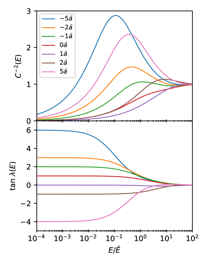
Figure 2: QDT functions $C^{-2}(E)$ and $\tan\lambda(E)$ for various background scattering lengths $a_{\textrm{bg}}$.

Examples of $C^{-2}(E)$ and $\tan\lambda(E)$ are shown in Fig. 2 for a variety of values of $a_{\textrm{bg}}$. The functions $C^{-2}(E)$ approach 1 at high energy, but at low energy the leading term is $k\bar{a}[1+(1-r_{\textrm{bg}})^{2}]$, so is the same for $a_{\textrm{bg}}=0$ and $2\bar{a}$. For larger values of $|r_{\textrm{bg}}|$, $C^{-2}(E)$ rises more rapidly and has a prominent peak; for $|r_{\textrm{bg}}|\leq 1$, this peak is small or absent. The functions $\tan\lambda(E)$ are $1-r_{\textrm{bg}}$ at low energy and approach zero at high energy; they start to decrease at substantially lower energies for larger values of $|r_{\textrm{bg}}|$. For $a_{\textrm{bg}}=\bar{a}$, $\tan\lambda(E)$ remains small at all energies.

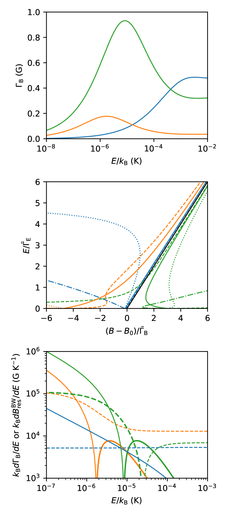
Figure 3: Resonance parameters for resonances 1 (blue), 3 (orange), and 4 (green). (a) Width $\Gamma_{\textrm{B}}(E)$. (b) $B_{\textrm{res}}^{\textrm{BW}}(E)$ (solid lines), $B_{\textrm{res}}^{\textrm{pole}}(E)$ (dotted lines), and peak and trough in $Q(E,B)$ (dashed and dot-dashed lines, respectively). The axes are scaled such that the bare bound state (black line) coincides for all three resonances. (c) Energy derivatives $d\Gamma_{\textrm{B}}/dE$ (solid lines) and $dB_{\textrm{res}}/dE$ (dashed lines); thicker lines show the absolute values when the quantities are negative.

Figure 3 shows the resonance parameters $\Gamma_{\textrm{B}}(E)$ and $B_{\textrm{res}}^{\textrm{BW}}(E)$ obtained from Eqs. (12) to (15) for resonances 1, 3, and 4, together with their energy derivatives. Panel (a) shows the width $\Gamma_{\textrm{B}}(E)$; the shapes are the same as those of the corresponding functions $C^{-2}(E)$ in Fig. 2. $\Gamma_{\textrm{B}}(E)$ for resonances 3 and 4 is greatly enhanced around a few $\mu$K before reducing at higher energies. The high-energy limits are the values of $\bar{\Gamma}_{\textrm{B}}$; this is larger for resonance 1 than for resonance 4, even though $\Delta$ is a factor of 6 smaller for resonance 1. Similarly, the high-energy limit of $\Gamma_{\textrm{B}}(E)$ is much smaller for resonance 3 than for resonance 1, even though $\Delta$ is similar for these two resonances. These effects arise because $|a_{\textrm{bg}}|$ is large for resonances 3 and 4, enhancing their widths near threshold.

The solid colored lines in Figure 3(b) show $B_{\textrm{res}}^{\textrm{BW}}(E)$ for the same three resonances; the axes are scaled by the short-range widths $\bar{\Gamma}_{\textrm{B}}$ and $\bar{\Gamma}_{\textrm{E}}=\mu_{\textrm{rel}}\bar{\Gamma}_{\textrm{B}}$, so that the bare bound states coincide (black line). For resonance 1, $B_{\textrm{res}}^{\textrm{BW}}(E)$ is close to the bare bound state; this is because $a_{\textrm{bg}}$ is close to $\bar{a}$ so that $\tan\lambda(E)$ is always small. For resonances 3 and 4, the deviations are much larger due to the large magnitudes of $a_{\textrm{bg}}$ and resulting large $\tan\lambda(E)$. The slopes $dB_{\textrm{res}}^{\textrm{BW}}/dE$ are constant in the low-energy limit, but very different from that of the bare bound state. For resonance 4 the slope at low energy has opposite sign to that at high energy because $a_{\textrm{bg}}$ is large and negative. The differences between $B_{\textrm{res}}^{\textrm{BW}}(E)$ and the position of the bare bound state descrease rapidly with energy

The dashed and dot-dashed lines in Figure 3(b) show the positions of the peaks and troughs in the time delay $Q(E,B)$, respectively . These both coincide with $B_{\textrm{res}}^{\textrm{BW}}(E)$ at zero energy, but they separate rapidly with increasing energy, by a quantity proportional to $E^{3/2}$. For resonance 1 the peak is very close to $B_{\textrm{res}}^{\textrm{BW}}(E)$; for resonance 3 it still approaches $B_{\textrm{res}}^{\textrm{BW}}(E)$ at high energy, though in a more complicated manner. For both these resonances the trough moves quickly away from $B_{\textrm{res}}^{\textrm{BW}}(E)$ as it becomes shallow and unimportant. For resonance 4 it is the trough that remains near $B_{\textrm{res}}^{\textrm{BW}}(E)$ at low energy, while the peak moves quickly away to high field and loses its identity. A new peak then approaches from the low-field side and replaces the trough near $B_{\textrm{res}}^{\textrm{BW}}(E)$.

The dotted lines in Figure 3(b) show the positions $B_{\textrm{res}}^{\textrm{pole}}(E)$ of the poles in the scattering length. They coincide with $B_{\textrm{res}}^{\textrm{BW}}(E)$ at zero energy, but move away from it rapidly as energy increases. They are unrelated to the peaks and troughs in the time delay. They exhibit divergences in field as a function of energy; these occur because $a_{\textrm{bg}}$ has a pole at every energy where the background phase shift $\delta_{\textrm{bg}}(E)$ passes through $(2n+1)\pi/2$, and $B_{\textrm{res}}^{\textrm{pole}}(E)$ undergoes a series of avoided crossings with these background poles.

Figure 3(c) shows the energy derivatives of $B_{\textrm{res}}^{\textrm{BW}}(E)$ and $\Gamma_{\textrm{B}}(E)$. At low energy, $dB_{\textrm{res}}^{\textrm{BW}}/dE$ is constant and $d\Gamma_{\textrm{B}}/dE$ is proportional to $E^{-1/2}$. For resonance 1 they remain close to their high- and low-energy limiting forms respectively, validating the approximations used to derive Eq. (11) for $E_{\textrm{X}}$; the two derivatives cross near $7\ \mu\textrm{K}$ as predicted. For resonances 3 and 4, however, $dB_{\textrm{res}}^{\textrm{BW}}/dE$ is dominated by threshold effects at low energy. The functions do not approach their high-energy behavior $dB_{\textrm{res}}^{\textrm{BW}}/dE=1/\mu_{\textrm{rel}}$ until $10\ \mu\textrm{K}$ or more. By contrast, $d\Gamma_{\textrm{B}}/dE$ deviates from its low-energy limiting behavior well below $10\ \mu\textrm{K}$. Both approximations used to derive Eq. (11) thus break down for these resonances. The behavior of $Q(E,B)$ can nevertheless be understood from the derivatives in Figure 3(c). In particular, it may be seen that for resonance 3 there is a single crossover between $dB_{\textrm{res}}^{\textrm{BW}}/dE$ and $d\Gamma_{\textrm{B}}/dE$, so that there is a well-defined value of $E_{\textrm{X}}$, even though it is poorly approximated by Eq. (11) in this case. For resonance 4, however, there are multiple crossovers and $E_{\textrm{X}}$ is poorly defined.

V Conclusions

We have studied the behavior of the collisional time delay in cold and ultracold atomic and molecular collisions. We have carried out coupled-channels scattering calculations on ultracold collisions of ⁸⁷Rb, ⁸⁵Rb and ¹³³Cs in the vicinity of magnetically tunable Feshbach resonances. Far above threshold, the time delay as a function of either energy or applied field exhibits a symmetric peak whose integral is independent of the resonance width. In the low-energy limit, however, the time delay is proportional to the scattering length (and inversely proportional to the collision velocity or wave vector $k$). Across a resonance, the scattering length passes through a pole as a function of applied field; there are regions of large positive and large negative time delay, and the resonant contribution averages to zero when integrated over the field.

For resonances that are narrow, or have a background scattering length $a_{\textrm{bg}}$ close to the mean scattering length $\bar{a}$, the transition from the low-energy oscillation to the high-energy peak occurs around a crossover energy $E_{\textrm{X}}$ that is proportional to the square of the dimensionless resonance strength parameter $s_{\textrm{res}}$. For broad resonances where $a_{\textrm{bg}}$ is large (either positive or negative), the behavior is more complex.

The behavior of the time delay at low energy arises from the variation of the resonance position and width near a scattering threshold. We have presented an analysis based on multichannel quantum defect theory. For narrow resonances and when $a_{\textrm{bg}}\approx\bar{a}$, the resonance position depends nearly linearly on energy and the main threshold effect is from the energy dependence of the resonance width. For broad resonances with $a_{\textrm{bg}}\gg\bar{a}$ or $a_{\textrm{bg}}\ll\bar{a}$, however, there are important additional effects due to the effect of the threshold on the resonance position.

The results obtained here will be conceptually important in understanding complex formation during ultracold collisions, which is believed to play an important role in losses of nonreactive molecules from traps. The resonances considered have comparable short-range widths to those predicted for collisions of ultracold molecules Christianen et al. (2019a).