Probing CO and N₂ Snow Surfaces in Protoplanetary Disks with N₂H⁺ Emission

Abstract

Snowlines of major volatiles regulate the gas and solid C/N/O ratios in the planet-forming midplanes of protoplanetary disks. Snow surfaces are the 2D extensions of snowlines in the outer disk regions, where radiative heating results in a decreasing temperature with disk height. CO and N₂ are two of the most abundant carriers of C, N and O. N₂H⁺ can be used to probe the snow surfaces of both molecules, because it is destroyed by CO and formed from N₂. Here we present Atacama Large Millimeter/submillimeter Array (ALMA) observations of N₂H⁺ at $\sim$0$\farcs$2–0$\farcs$4 resolution in the disks around LkCa 15, GM Aur, DM Tau, V4046 Sgr, AS 209, and IM Lup. We find two distinctive emission morphologies: N₂H⁺ is either present in a bright, narrow ring surrounded by extended tenuous emission, or in a broad ring. These emission patterns can be explained by two different kinds of vertical temperature structures. Bright, narrow N₂H⁺ rings are expected in disks with a thick Vertically Isothermal Region above the Midplane (VIRaM) layer (LkCa 15, GM Aur, DM Tau) where the N₂H⁺ emission peaks between the CO and N₂ snowlines. Broad N₂H⁺ rings come from disks with a thin VIRaM layer (V4046 Sgr, AS 209, IM Lup). We use a simple model to extract the first sets of CO and N₂ snowline pairs and corresponding freeze-out temperatures towards the disks with a thick VIRaM layer. The results reveal a range of N₂ and CO snowline radii towards stars of similar spectral type, demonstrating the need for empirically determined snowlines in disks.

1 Introduction

Snow lines, the transition regions in disk midplanes where volatiles such as H₂O, CO₂, and CO freeze out from the gas phase onto dust grains, may affect planet formation through several different channels. Snow lines can locally enhance particle growth, boosting planetesimal formation efficiencies at specific radii through a combination of (1) increases in solid mass surface density exterior to snow line locations, (2) “cold-head effects” that transport volatiles across snow lines, (3) pile-ups of dust just inside of the snow line in pressure traps, and (4) an increased “stickiness” of icy grains at the H₂O snow line compared with bare particles (Ciesla & Cuzzi, 2006; Johansen et al., 2007; Chiang & Youdin, 2010; Gundlach et al., 2011; Ros & Johansen, 2013; Xu et al., 2017). Snow lines also regulate the bulk elemental composition of planets and planetesimals, including the elemental C/N/O ratios (Öberg et al., 2011a; Öberg & Bergin, 2016; Piso et al., 2016).

Snowline locations can in principle be calculated using known disk midplane density and temperature structures, and volatile desorption and adsorption rates. Desorption rates depend sensitively on volatile binding energies, however, and laboratory experiments have demonstrated that CO and N₂ binding energies can vary by up to 50%, depending on the structure and composition or water content of the ice they are adsorbed on (Fayolle et al., 2016). For the pressures present in disks, CO can therefore freeze out anywhere from $\sim$21 to 32 K, and N₂ between $\sim$18 and 27 K (Collings et al., 2004; Öberg et al., 2005; Bisschop et al., 2006; Fayolle et al., 2016). Furthermore disk snowline locations are affected by the dynamics of the gas and dust. Pebble drift is especially relevant, since it can move snowlines closer to the star than would be expected from desorption-adsorption balance in static disks (Piso et al., 2015). Accurate snowline predictions are therefore not possible, and we instead rely on observations of snowlines to benchmark disk models.

Direct observations of snowlines through the identifications of sharp radial drop-offs in emission from the snowline volatile is challenging for CO and impossible for N₂. The latter prohibition is due to N₂’s lack of dipole moment, and therefore lack of observable rotational lines. Optically thin isotopologues of CO can be used to constrain the CO snowline location (Qi et al., 2011; Schwarz et al., 2016; Huang et al., 2016; Zhang et al., 2017), but it is difficult to distinguish between a decreasing gas surface density or CO abundance without independent constraints on the former. This issue is compounded by vastly different disk temperature structures, which can make the expected CO emission drop at the CO snowline quite subtle (see discussions in Section 4.3).

An alternative approach to constrain snowline locations is to image the distribution of a chemically related species, whose abundance is connected to the freeze-out of the desired volatile through a simple set of chemical reactions. N₂H⁺ has been used to chemically image CO snowlines, exploiting the fact that N₂H⁺ is quickly destroyed by gas-phase CO and therefore only expected to be present in disks exterior to the CO midplane snowline (Qi et al., 2013). The distribution of N₂H⁺ also depends on the N₂ snowline location since it forms through proton transfer from H${}_{3}^{+}$ to N₂. In cloud cores the depletion of N₂H⁺ at low temperatures has indeed been successfully used to constrain N₂ freeze-out locations (Bergin et al., 2002), but it has not yet been attempted in disks.

Interpretation of chemical images of snowlines is not always expected to be straightforward, however. van ’t Hoff et al. (2017) modeled the relationship between CO freeze-out and N₂H⁺ emission and found that the N₂H⁺ emission peaks exterior to the CO snowline because of CO sublimation and N₂H⁺destruction in the warmer layers immediately above the midplane (see Figure. 5 in van ’t Hoff et al., 2017). The disk height at which CO sublimates into the gas-phase above the CO midplane snowline depends on the steepness of the disk vertical temperature gradient. The relationship between the N₂H⁺ morphology and the CO snowline location, and therefore whether N₂H⁺ imaging can be used to efficiently constrain the CO (and N₂) snowlines is then closely related to the disk vertical temperature structure.

Here we present Atacama Large Millimeter/submillimeter Array (ALMA) observations of N₂H⁺ $3-2$ emission around 279.5 GHz at $\sim$0$\farcs$2–0$\farcs$4 resolution in the disks around LkCa 15, GM Aur, DM Tau, V4046 Sgr, AS 209 and IM Lup. These disks span a range of disk thermal vertical structure and therefore present a perfect test-bed for the utility of N₂H⁺ in probing N₂ and CO snowlines in different kinds of disks. We describe the sample and observations in Section 2, present the results and analysis in Section 3 and discussions in Section 4, and summarize our conclusions in Section 5.

2 Observations

2.1 Sample selection

Table 1: Stellar Properties

Sourcea	R.A.	Decl.	L∗	Age	M∗b	$\dot{M}$	Teff	Distance
	(J2000)	(J2000)	(L⊙)	(Myr)	(M⊙)	(10-9M⊙ yr-1)	(K)	(pc)
LkCa 15	04 39 17.80	+22 21 03.1	1.0	2.0	1.2	6.3	4365	158
GM Aur	04 55 10.99	+30 21 59.0	1.6	2.5	1.2	7.9	4786	159
DM Tau	04 33 48.75	+18 10 09.7	0.24	4.0	0.52	4.0	3715	145
V4046 Sgr	18 14 10.48	-32 47 35.4	0.49,0.33	24	1.75	0.5	4370	72
AS 209	16 49 15.30	-14 22 09.0	1.4	1.0	0.83	50	4266	121
IM Lup	15 56 09.2	-37 56 6.5	2.6	0.5	0.89	13	4365	158

Note. — ^a The source information are from Andrews et al. (2018a) and the references within, except for V4046 Sgr from Huang et al. (2017) and the references within. ^b Stellar masses for LkCa 15, GM Aur and DM Tau are fit, given the inclination determined from the continuum fitting.

The disk sample consists of 6 T Tauri disks, which constitute a sub-set of the 12 disks observed in a multitude of molecular lines with the SMA as part of the DISCS survey (Öberg et al., 2010, 2011b). Six of the DISCS targets were detected in N₂H⁺ by the SMA and these constitute our sample. It consists of four T Tauri stars with large central cavities in millimeter dust emission (LkCa 15, GM Aur, DM Tau, V4046 Sgr) and two T Tauri stars without such cavities (AS 209 and IM Lup). Table 1 shows the detailed stellar properties for the 6 sources.

2.2 Observation setup

Table 2: ALMA observation details

Source	Date	Antennas	Baselines	On-source	Bandpass	Phase	Fluxb
			(m)	integration (min)	Calibrator	Calibrator	Calibrator
LkCa15/GM Aura	2016 July 27	45	15-1100	19/17	J0510+1800	J0433+2905	J0510+1800 (1.443 Jy)
	2016 August 16	42	15-1500	19/17	J0510+1800	J0433+2905	J0510+1800 (1.554 Jy)
	2016 August 22	40	15-1500	19/17	J0510+1800	J0433+2905	J0423-0120 (0.442 Jy)
DM Tau	2016 August 31	39	15-1800	53	J0510+1800	J0431+2037	J0238+1636 (0.961 Jy)
V4046 Sgr	2016 April 30	41	16-640	20	J1924-2914	J1802-3940	Titan
AS 209	2016 June 09	38	16-783	64	J1517-2422	J1733-1304	J1733-1304 (1.618 Jy)
	2016 August 26	42	15-1500	32	J1517-2422	J1733-1304	J1733-1304 (1.555 Jy)
IM Lup	2016 June 09	38	16-783	29	J1517-2422	J1604-4441	J1517-2422 (2.265 Jy)

Note. — ^a LkCa 15 and GM Aur were observed in the same scheduling blocks.^b Quasar flux averaged over all the spectral windows

The six disks were observed during ALMA Cycle 3 (project code [ADS/JAO.ALMA#2015.1.00678.S]) in Band 7 with a single spectral set-up consisting of 6 spectral windows with widths and resolutions ranging from 117.2 to 937.5 MHz, and 122.1 to 976.6 khz respectively. The N₂H⁺ $3-2$ line was place in a 117.2 MHz wide spectral window with a native resolution of 122.1 khz (0.13 km s^-1). Additional windows covered the DCO⁺ 4–3 and H₂CO 6_0,6–5_0,5 lines. The DCO⁺ data will be presented in a future paper, and the H₂CO data is presented in Pegues et al. (subm.). V4046 Sgr data were also presented in Kastner et al. (2018). The array configuration and calibrators for each observation are described in Table 2.

2.3 Data reduction

ALMA/NAASC staff performed the standard pipeline calibration tasks. Subsequent data reduction and imaging were completed with CASA 4.7.0 (McMullin et al., 2007). For each disk, the data were separated with the spectral windows in the upper and lower sideband. For each sideband, the corresponding continuum was phase self-calibrated by combining the line-free channels of the spectral windows and then imaged by CLEANing with a robust parameter of 0.5. The self-calibrated tables were subsequently applied to the spectral windows for each sideband, and the 284 GHz continuum was obtained by combining the linefree channels of both sidebands. Table 3 lists the fluxes, rms values, beam sizes and position angles, as well as the disk inclinations and position angles. The latter two are based on Gaussian fits to the disk continuum: we determine the position angle of the disk major axis (measured east of north) and the disk inclination (0 is face-on) by fitting an elliptical Gaussian component on the high SNR continuum image using the CASA task IMFIT. The values for AS 209 and IM Lup are consistent with those in Huang et al. (2018) derived from deeper ALMA observations with much higher angular resolution. The radius of the millimeter dust continuum was estimated by the size of the 3$\sigma$ contour of the image in the direction of the disk major axis.

Table 3: Properties of the 284 GHz dust continuum and derived disk properties

Source	Fconta	Peak flux densitya	Beam (P.A.)	Disk Incl.	Disk P.A.	Radius ($3\sigma$
	(mJy)	(mJy beam-1)		(deg)	(deg)	(au)
LkCa 15	281.0$\pm$6.9	13.01$\pm$0.31	$0\farcs.25\times 0\farcs 22$ (-18∘.2)	50.5${}^{+2.3}_{-2.4}$	61.4$\pm$2.1	230
GM Aur	286.4$\pm$2.6	22.27$\pm$0.19	$0\farcs 29\times 0\farcs 18$ (-1∘.6)	51.9${}^{+0.8}_{-0.9}$	56.5$\pm$0.8	300
DM Tau	99.1$\pm$1.4	12.38$\pm$0.15	$0\farcs 21\times 0\farcs 18$ (-177∘.9)	36.3${}^{+2.3}_{-2.4}$	157.6$\pm$2.9	240
V4046 Sgr	576$\pm$12	49.58$\pm$0.97	$0\farcs 38\times 0\farcs 29$ (-73∘.1)	33.6${}^{+2.8}_{-4.0}$	74.5$\pm$5.7	110
AS 209	289.0$\pm$4.5	40.45$\pm$0.56	$0\farcs 32\times 0\farcs 21$ (-70∘.9)	35.0${}^{+2.8}_{-3.1}$	90.5$\pm$4.1	180
IM Lup	243.7$\pm$6.2	54.1$\pm$1.1	$0\farcs 40\times 0\farcs 33$ (82∘.6)	44.2${}^{+3.5}_{-3.9}$	139.9$\pm$5.0	360

Note. — ^aUncertainties do not include 10% systematic flux uncertainties.

After self-calibration, the continuum were subtracted in the $uv$-plane from the spectral windows containing N₂H⁺. Then the data were binned at 0.15 km s^-1 and output to UVFITS file. Then UVFITS files were loaded into MIRIAD (Sault et al., 1995) for imaging. All N₂H⁺ line observations were CLEANed with a Briggs parameter of 2.0 for optimal sensitivity.

3 Results and Analysis

Table 4: Line Observations

Source	Integration range	Channel rms	Mask axis	Integrated flux	Beam (P.A.)
	(km s-1)	(mJy beam-1)	(′′)	(mJy km s-1)
LkCa 15	2.7–10.2	3.2	6	1820 $\pm$ 23	$0\farcs 32\times 0\farcs 29$ (-23∘.0)
GM Aur	1.6–9.4	3.2	6	1487 $\pm$ 23	$0\farcs 36\times 0\farcs 24$ (-3∘.0)
DM Tau	4.5–8.0	4.1	6	1286 $\pm$ 40	$0\farcs 30\times 0\farcs 28$ (8∘.1)
V4046 Sgr	-0.9–7.2	5.4	8	3761 $\pm$ 81	$0\farcs 59\times 0\farcs 49$ (-78∘.5)
AS 209	1.9–7.9	2.7	4	917 $\pm$ 15	$0\farcs 42\times 0\farcs 27$ (-70∘.3)
IM Lup	1.8–7.5	4.5	6	2040 $\pm$ 49	$0\farcs 49\times 0\farcs 41$ (88∘.1)

Note. — Column descriptions: (1) Source name. (2) Velocity range integrated across to calculate integrated flux. (3) Channel rms for bin size of 0.15 km s^-1. (4) Major axes of elliptical spectral extraction masks. (5) Integrated flux. Uncertainties do not include systematic flux uncertainties. (6) Synthesized beam dimensions

3.1 Observational results

Figure 1 shows the 284 GHz continuum and the integrated intensity maps and spectra of N₂H⁺ $3-2$ towards the six disks. The central dust cavities reported in LkCa 15, GM Aur, DM Tau, V4046 Sgr (Hughes et al., 2009; Rosenfeld et al., 2013; Andrews et al., 2011; Huang et al., 2017) are resolved in the 284 GHz continuum. The multi-ringed dust structure resolved in the continuum of AS 209 is also consistent with those shown in Huang et al. (2017); Fedele et al. (2018); Guzmán et al. (2018).

The N₂H⁺ integrated intensity maps (second row in Figure 1) were produced by summing over channels in velocity ranges listed in Table 4, corresponding to where N₂H⁺ emission was detected above the 2-3$\sigma$ level. The N₂H⁺ spectra (third row in Figure 1) were extracted from the image cubes (shown in the Appendix) using elliptical regions with centroid of the continuum image and shapes and orientations based on the inclination and position angle for each disk (Table 3). The major axis of the elliptical region (Table 4) is chosen to cover the $>3\sigma$ line emission in the image cubes. The uncertainties are treated the same way as described in Huang et al. (2017, Section 3.2). Finally, Figure. 2 shows the corresponding deprojected and azimuthally averaged radial profiles for each disk, assuming the position angles and inclinations listed in Table 3.

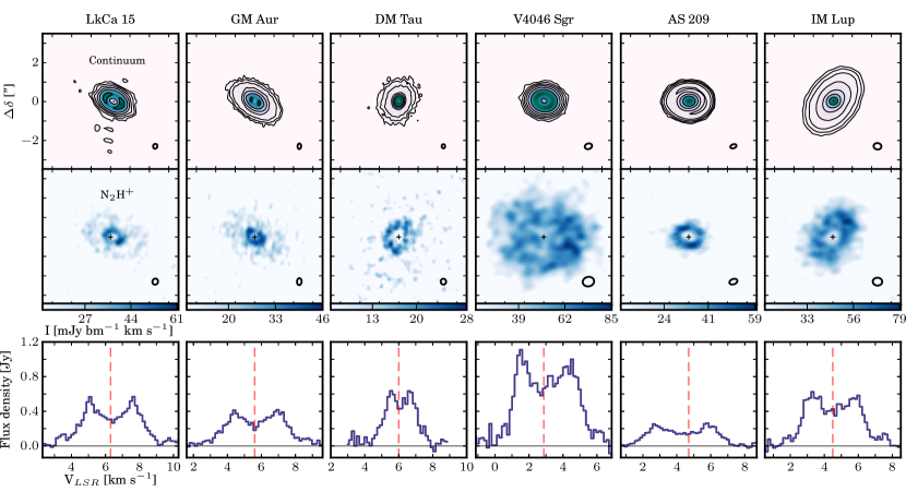
Figure 1: Continuum images and N₂H⁺ $3-2$ integrated intensity maps and spectra. First row: intensity maps of the 284 GHz dust continuum. Contours are drawn at [5, 10, 20, 40, 80, 160…]$\sigma$, where $\sigma$ is the rms listed in Table 3. Note the continuum sub-structure in the LkCa 15, GM Aur, DM Tau and AS 209 disks. Second row: integrated intensity maps of N₂H⁺ $3-2$. Color bars start at 2$\sigma$, where $\sigma$ is the rms of the integrated intensity map. Synthesized beams are drawn in the lower right corners of each panel. The centroid of the continuum image is marked with a cross. Offset from the centroid in arcseconds is marked on the y axis of the upper left corner panel. The N₂H⁺ maps display a range of morphologies from narrow to broad rings. Third row: Spectra of N₂H⁺ $3-2$ show the double-peaked shape characteristic of a Keplerian rotation disk. Even though there are 29 hyper-fine components for the N₂H⁺ $3-2$ line (see Appendix), the dominant components spread less than 0.4 km s^-1. The vertical red line marks the systemic velocity.

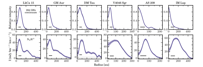
Figure 2: Deprojected and azimuthally averaged 284 GHz continuum intensity and integrated N₂H⁺ $3-2$ line intensity radial profiles. Top row: continuum intensity profiles normalized to peak values. Bottom row: radial profiles of integrated line intensity. The color shades show the standard deviation in pixel intensities calculated at each annulus. Adopted distances are listed in Table 1, and adopted position angles and inclinations are listed in Table 3. Black bars in each panel represent the restoring beam major axes. Note the distinct N₂H⁺ morphologies in the three leftmost disks – a narrow ring followed by a low-level plateau, and the three rightmost disks – a broad torus more extended than the continuum disk.

Based on the integrated intensity maps and radial profiles, the morphologies of the N₂H⁺ emission can be divided into two distinct groups: (1) a bright, narrow ring surrounded by tenuous extended emission in the disks of LkCa 15, GM Aur, and DM Tau; (2) a broad torus extending across the dust disk for V4046 Sgr, AS 209, and IM Lup. At first glance, AS 209 seems to straddle these two categories, but its N₂H⁺ emission is “broad” compared to its compact continuum, placing it in the second group.

A second, tenuous ring of N₂H⁺ can be seen in the disks of LkCa 15 (at $\sim$220 au), GM Aur ($\sim$200 au), and IM Lup ($\sim$350 au) in the radial profiles (and also in the channel maps). In all sources the second ring appears to be close to the edge of the mm dust continuum emission (Table 3). In the case of IM Lup and LkCa 15, the second N₂H⁺ ring resides somewhat exterior to the second rings of H¹³CO⁺ and DCO⁺ in the same disk: 310 au for IM Lup; 200 au for LkCa 15 (Huang et al., 2017), possibly related to CO desorption at these large radii. The spatial coincidence between this second N₂H⁺ ring and the continuum edge suggests that its appearance is due to an increased radiation penetration towards the disk midplane beyond the pebble edge. Enhanced radiation can cause a thermal inversion (Cleeves, 2016), resulting in N₂ and CO desorption, and should also increase the ionization level (Bergin et al., 2016), which may promote N₂H⁺ production. The displacement between the second ring of N₂H⁺ and that of H¹³CO⁺ and DCO⁺ indicates a possible thermal inversion near or beyond the pebble edge.

3.2 Effects of vertical temperature profiles on N₂H⁺ emission

In this paper, we argue that the morphology differences of N₂H⁺ emission depend mainly on the disk vertical temperature structure. In the outer disk (beyond 10 au), the disk radial-vertical temperature structure is generally set by the radiation heating and dust growth/settling. The temperature decreases deeper in the disk since the stellar radiation is deposited in the atmosphere and reprocessed to lower energy photons that warm the disk interior. Near the midplane (z=0) where the disk is optically thin to its own radiation, the temperature is approximately constant with height, maintained by the reprocessed flux reaching to this layer, resulting in a Vertically Isothermal Region above the Midplane (VIRaM) layer. The height of this layer can vary substantially from disk to disk; the isothermal layer extends higher for disks that have more small grains that trap radiation at surface, whereas the isothermal layer is lower for more settled disks (i.e., large dust grains are more concentrated towards the midplane (see Figure. 5 in D’Alessio et al., 2006)). Above the VIRaM exterior to the CO midplane snowline, there is a vertical layer where N₂ is in the gas-phase, while CO is not.

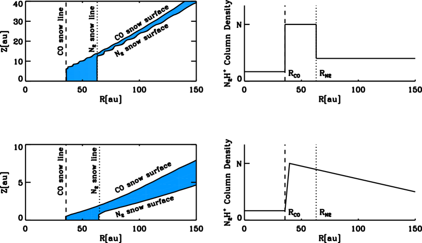
Figure 3: Schematic representation of the effects of vertical temperature structures on the N₂H⁺ emission. Left panels: The snow surfaces of CO and N₂ in the disks with same midplane temperatures but different vertical temperature structures; in the upper panel the VIRaM layer extends through a substantial part of the disk, while in the lower panel the VIRaM layer is thin, and instead there is a vertical temperature gradient from the midplane to the disk surface. The solid blue shows the disk regions where N₂ is in the gas-phase and CO is frozen out, and thus where N₂H⁺ should be abundant. Right panels: The expected corresponding N₂H⁺ column density distributions. The thick VIRaM layer case results in sharp edges at the CO and N₂ midplane snowline, while the opposite is true for disks with a thin VIRaM layer.

We expect N₂H⁺ to trace the CO and N₂ snow surfaces – the 2D iso-temperature contours that correspond to freeze-out temperature of CO and N₂ across the disk. Figure 3 visualizes the impact of different disk vertical temperature structures on the N₂H⁺ radial column density profile. For disks with a thick VIRaM layer (upper panels), the CO and N₂ snow surfaces extend vertically from the midplane snowlines and we expect the N₂H⁺ emission to present a bright, and narrow ring, with inner and outer radii constrained by the two snowlines. Beyond the N₂H⁺ midplane snowline we expect some tenuous emission originating from higher disk layers where N₂H⁺ exists in between the CO and N₂ snow surfaces. Because of a steep temperature gradient at these disk heights, and a comparably small difference in freeze-out temperature between CO and N₂, this contribution should be small and readily distinguishable from the emission component marking the CO and N₂ snowlines.

The lower panels of Figure. 3 show that for disks with a thin VIRaM layer the N₂H⁺ emission profile traces the CO midplane snowline more indirectly and the N₂ snowline not at all. In such disks, snow surfaces are non-vertical resulting in an offset between the CO snowline and the inner edge of N₂H⁺ emission, as described by van ’t Hoff et al. (2017). The connection between the N₂H⁺ emission and the N₂ snowline is completely washed out because the vertical layer where N₂H⁺ can exist above the CO snow surface is thick compared to the VIRaM layer. Observationally disks of this kind should present broad N₂H⁺ rings with inner edges slightly beyond the CO snowline and outer edges limited by total disk column density fall-offs in the outer disks.

3.3 Disk vertical temperature structure models

The two groups of observed N₂H⁺ emission morphologies resemble those expected from disks with a thick or thin VIRaM layer (Figure. 3). To test whether the observed disks do fall into the two groups, and to retrieve snowline locations in disks with a thick VIRaM layer, we use the D’Alessio Irradiated Accretion Disk (DIAD) code (D’Alessio et al., 1998, 1999, 2001, 2005, 2006) to model the disks, with special focus on the disk vertical temperature structures.

DIAD considers a flared irradiated accretion disk in hydrostatic equilibrium and the radial and vertical structure of the disks are calculated self-consistently. For a given mass accretion rate ($\dot{M}$), and viscosity coefficient ($\alpha$), the density and temperature structure of this model is determined as described by D’Alessio et al. (1998, 1999). We consider heating from the mechanical work of viscous dissipation (relevant only in the midplane of the inner disk), accretion shocks at the stellar surface, and passive stellar irradiation, and follow the radiative transfer of that energy with 1+1D calculations using the Eddington approximation and a set of mean dust opacities (gas opacities are considered negligible). The dust is assumed to be a mixture of segregated spheres composed of “astronomical” silicates and graphite, with abundances (relative to the total gas mass) of $\zeta_{\rm sil}=0.004$ and $\zeta_{\rm gra}=0.0025$ (Draine & Lee, 1984): the “reference” dust-to-gas mass ratio is $\zeta_{\rm ref}=0.0065$. At any given location in the disk, the grain size ($a$) distribution of these dust particles is assumed to be a power-law, $n(a)\propto a^{-3.5}$, between $a_{\rm min}=0.005$ $\mu$m and a specified $a_{\rm max}$.

Figure 4: Spectral energy distributions (SEDs) of the six disks and the best fit models used to constrain the vertical disk temperature structures. The black points and error bars represent the measured photometry and the red line shows the IRS spectra. The blue lines represent the stellar photosphere, the green lines are the disk models and the purple lines show the total emission of the model.

Table 5: SED fitting parameters

	Outer Disk						Inner Wall				Optically Thin Dust Region
Source	$\epsilon$	$\alpha$	Twall	Rwalla	Hwall	amax	Twallb	Rwalla	Hwall	amax	$\tau$	Rin	Rout	amax
			(K)	(au)	(au)	($\mu$m)	(K)	(au)	(au)	($\mu$m)		(au)	(au)	($\mu$m)
LkCa 15	1.0	0.0001	95.0	68.75	1.8	0.25	1400	0.14	0.01	1.0	0.02	0.3	5.0	0.25
GM Aur	1.0	0.00045	120.0	29.95	1.9	3.0	-	-	-	-	0.007	0.1	3.0	0.1
DM Tau	0.5	0.0015	200.0	3.71	0.3	2.0	-	-	-	-	-	-	-	-
V4046 Sgr	0.01	0.0005	140.0	12.04	0.7	5.0	-	-	-	-	0.01	0.2	1.0	4.0
AS 209	0.001	0.015	400.0	3.58	1.1	0.25	1400	0.26	0.1	0.25	-	-	-	-
IM Lup	0.001	0.003	500.0	1.56	0.1	3.0	-	-	-	-	-	-	-	-

Note. — ^aR_wall is calculated using T_wall following D’Alessio et al. (2005). ^bWe set T_wall to an adopted dust sublimation temperature of 1400 K.

We tune 6-12 parameters for each object to fit its spectral energy distribution (SED; Table 5). The first 6 parameters in Table 5 pertain to the outer disk and are listed for each object. To achieve the best-fit, we test dust settling coefficient values ($\epsilon$) of 1.0, 0.5, 0.1, .01, and 0.001 and vary accretion as parameterized by $\alpha$ between 0.00001 – .02. The inner disk edge or “wall”, is modeled with temperature (T_wall) and the height (H_wall), which are varied to fit the SED. The radius of the wall is calculated using T_wall following D’Alessio et al. (2005). The maximum grain size in the disk atmosphere, a_max, was modeled as 0.1, 0.25, 1.0, 2.0, 3.0, 4.0, and 5.0 µm.

In the cases of LkCa 15 and AS 209, the SED can be better characterized with an additional inner disk component with an optically thick wall located at the dust sublimation radius. Here we adopt a dust sublimation temperature of 1400 K. In addition LkCa 15, GM Aur, and V4046 Sgr require some optically thin dust within their disk cavities to reproduce the SED. Following Espaillat et al. (2011), we vary $\tau$, the vertical optical depth evaluated at 10 µm, the inner and outer radii of the optically thin dust region (R_in, R_out), and a_max. The best-fit values are listed in Table 5 and Figure. 4 shows that the best-fit models yield excellent fits to the SEDs of the six disks. The stellar photosphere, and optically thin dust reproduce well the optical and near/mid-IR data, while the tuned disk models provide good fits to the longer wavelength SED points.

We note that this kind of SED fitting, especially to Spitzer IRS data points and the FIR wavelength region traced by Herschel, is highly sensitive to the vertical disk structure, the main goal of this study. The main regulating parameter for the disk vertical structure in the DIAD models is $\epsilon$, which describes the depletion of dust in the disk upper layers. All of our DIAD models are calculated using a mixture of two grain populations: small grains with a disk-specific max radius $a_{\rm max}$ (Table 5), and large grains with $a_{\rm max}=1$ mm. The latter grains are concentrated close to the disk midplane, within 10% of the local gas scale height $H$, i.e. the height of the transition between the small and big grains, z_big=0.1$H$. We keep the vertically integrated dust-to-gas ratio constant, which implies that any missing dust in the disk upper layers as parameterized by $\epsilon$ has been moved, or settled to the midplane. Formally we define $\epsilon=\zeta_{\rm small}/\zeta_{\rm std}$, where $\zeta_{\rm small}$ is the dust-to-gas mass ratio in the upper layers and $\zeta_{\rm std}$ is the standard dust-to-gas mass ratio in the interstellar medium (see the detailed dust settling prescription in D’Alessio et al. (2006)), i.e. the degree of settling increases as $\epsilon$ decreases.

Figure 5: Extracted disk temperature structures based on SED modeling. Note the different vertical scales in the upper vs lower panels. The disks in the upper panels all display substantial VIRaM layers, of $\sim$10 au around the CO and N₂ midplane the snowlines. By contrast the VIRaM layers in the disks in the lower panels are $<$1 au thick.

Table 5 shows that in our sample the key fitting parameter $\epsilon$ is either $\epsilon\geq 0.5$ (LkCa 15, GM Aur, and DM Tau) or $\epsilon\leq 0.01$ (V4046 Sgr, AS 209, and IM Lup). Figure. 5 shows the resulting vertical temperature structure of the disks, and its profound dependence on dust settling; the thickness of the VIRaM layer is more than an order of magnitude thicker in the disks with no settling, compared to the highly settled disks. This dependence can be understood when considering the radiative transfer of stellar radiation through the disk. As demonstrated in D’Alessio et al. (2006), close to the disk midplane the disk temperature decreases with height since less stellar energy reaches the lower layers. At the disk height where the disk becomes optically thin to its own radiation the midplane becomes nearly isothermal. For disks with a high dust content in their upper layers ($\epsilon\geq 0.5$), this transition takes place at high disk altitudes and the VIRaM layer is therefore thick, extending to $z/r\approx 0.2$. The result is nearly vertical temperature contours and therefore vertical snow surfaces for CO and N₂ from the disk midplane and up through most of the disk. For highly settled disks, stellar radiation can penetrate much deeper into the disk, and the transition to the optically thin, the isothermal disk layer takes place close to the disk midplane, at $z/r\approx 0.01$. As a result isotherms are highly inclined with respect to the surface normal through most of the disk, resulting in snow-surfaces that are highly inclined as well.

We note that the thickness of the VIRaM layer is sensitive to the distribution of the small grains in the disk. In the DIAD models, varying the parameter z_big, which is typically fixed to $0.1H$, should also affects the disk vertical temperature structure, as demonstrated in Qi et al. (2011). Besides gravitational settling, dust grain dynamics (e.g., radial drift, dust fragmentation), which are not yet considered in the DIAD models, should also change the spatial distribution of the small grains. We do not explore these effects here, as we do not expect a more detailed treatment will result in qualitative changes to the VIRaM structure of these disks.

3.4 Snowline(s) characteristics

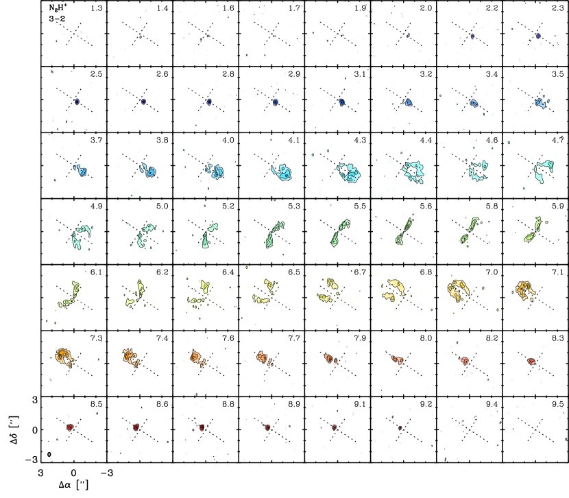
Figure 12: N₂H⁺ $3-2$ channel maps of the GM Aur disk.

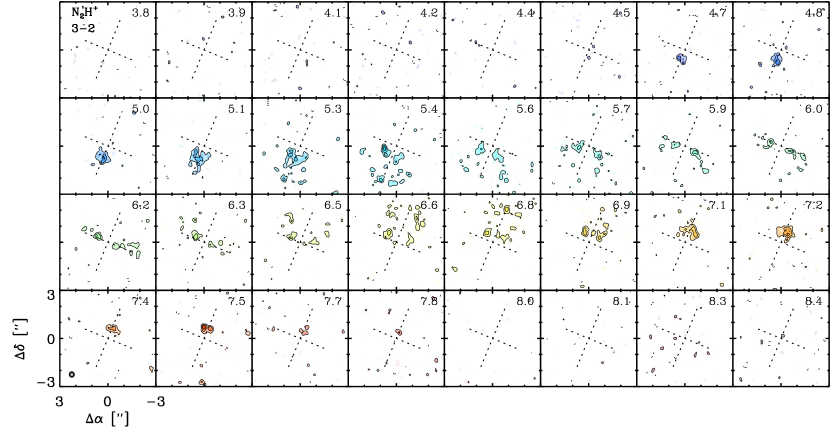
Figure 13: N₂H⁺ $3-2$ channel maps of the DM Tau disk.

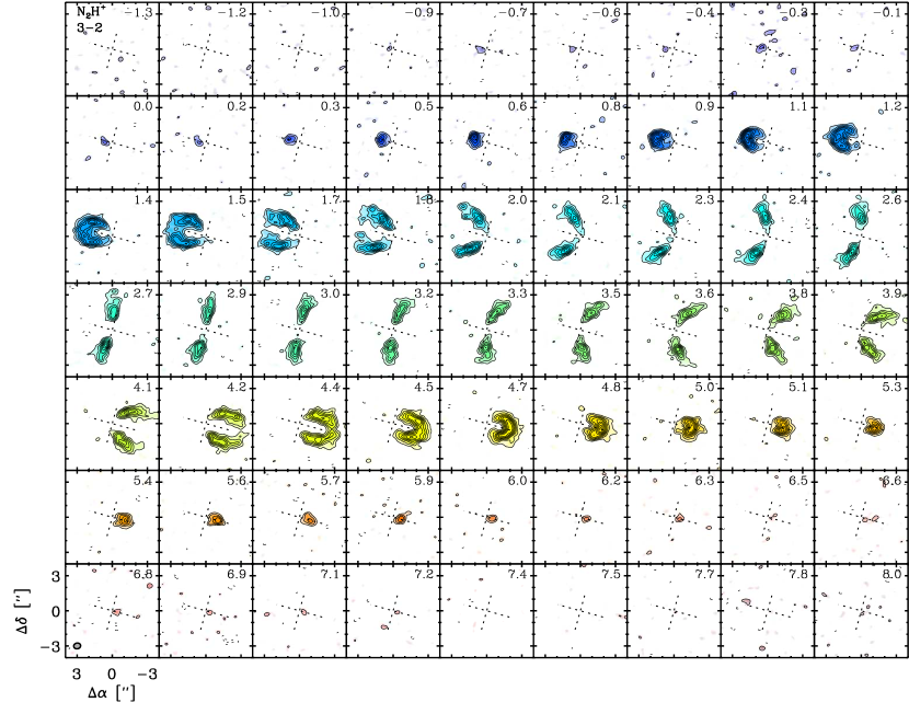
Figure 14: N₂H⁺ $3-2$ channel maps of the V4046 Sgr disk.

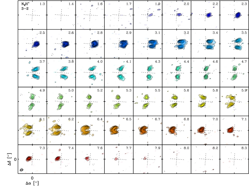
Figure 15: N₂H⁺ $3-2$ channel maps of the AS 209 disk.

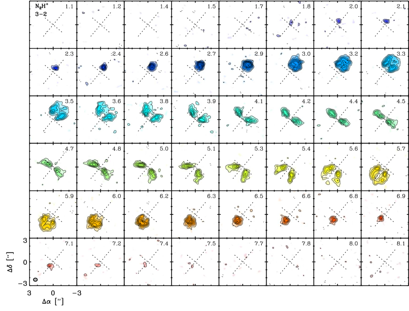
Figure 16: N₂H⁺ $3-2$ channel maps of the IM Lup disk.

N₂H⁺ emission morphologies in our disk sample all present as a ring structure, and the radial location of the inner edge of the ring should provide information about the CO snowline location. An initial estimate of the inner ring edge can be obtained through the detection of the N₂H⁺emission at the highest velocity channels which corresponds to the emission from the innermost radii considering the disk in Keplerian rotation. By measuring the velocity difference $\delta V$ (in unit of km s^-1) between the systemic velocity and the velocity in the most blue-shifted channel with $>3\sigma$ detection (See Figures 11-16 in the Appendix A), we derive the inner edge radii R (in unit of au) as $100\times M_{star}(\frac{2.98\sin{i}}{\delta V})^{2}$ where M_star is the stellar mass in unit of M_⊙ and $i$ is the inclination of the disk as listed in Tables 1 and  3. Inserting the values, we obtain the initial estimates of the inner edge of N₂H⁺ ring as 51, 41, and 72 au in the disks of LkCa 15, GM Aur, and DM Tau (first group) and 33, 31, and 59 au in the disks of V4046 Sgr, AS 209, and IM Lup (second group). As shown in Figure. 3, these values can be treated as the initial estimates of the CO snowline locations for the first group and the upper limits for the second one. Due to the lack of a thick VIRaM layer in the disks of the second group, the N₂ snowline cannot be constrained from the N₂H⁺ emission profiles. We note that the uncertainty in the velocity offset analysis described here is hard to determine, especially for the low inclination disk systems as it suffers more confusion from the hyper-fine components of the N₂H⁺ line. More rigorous constraints on the CO and N₂ snowline locations in the disk of the first group can be obtained using $\chi^{2}$ analysis of the visibilities in the $(u,v)$-plane.

It is a remarkable confirmation of disk chemistry theory that the disks in §3.3 that are modeled to have little settling and therefore a thick VIRaM layer perfectly overlap with the disks that present narrow and well-defined N₂H⁺ rings. In these three disks we expect near vertical CO and N₂ snow surfaces extending from the midplane and therefore the inner and outer edges of the N₂H⁺ ring should well isolate the CO and N₂ midplane snow lines, as shown schematically in Figure. 3. To derive snowline locations from the N₂H⁺ emission we use a parametric abundance model, with a “jump and drop” radial column density profile of N₂H⁺ (Figure. 6) to simulate the effects of freeze-out of gas-phase CO (producing the jump) and freeze-out of N₂ (producing the drop). The model parameters are the peak column density of N₂H⁺, N_p and the column density ‘jump’ factor J1 and ‘drop’ factor D2 at the corresponding inner and outer edges of the bright ring, R1 and R2, as well as an outer radius $R_{\rm out}$.

Figure 6: Schematic of the column density “jump and drop” model used to derived CO and N₂ snowline locations for disks with a thick VIRaM layer. R1 and R2 correspond to the CO and N₂ midplane snow-line locations, respectively, J1 is the N₂H⁺ enhancement following CO freeze-out in the midplane, and D2 the N₂H⁺ drop exterior to the N₂ snowline, where N₂H⁺ only exist in a thin, elevated disk layer.

In the vertical dimension, we follow the methodology of Qi et al. (2013, 2015) and assume that the N₂H⁺ abundance is constant between the disk surface ($\sigma_{s}$) and midplane ($\sigma_{m}$) boundaries at each radius. These boundaries are described in terms of $\Sigma_{21}=\Sigma_{H}/(1.59\times 10^{21}{\rm cm}^{-2})$, where $\Sigma_{H}$ is the hydrogen column density (measured downward from the disk surface) in the adopted physical model. We fix the boundary values to be 3.2 and 100, appropriate for a disk midplane tracer like N₂H⁺ according to e.g., the chemical models of Aikawa & Nomura (2006, Figure. 8). The abundance at any one radius is then completely described by the N₂H⁺ column density model described above and the given disk density model.

We use the 2D Monte Carlo software RATRAN (Hogerheijde & van der Tak, 2000) to calculate the radiative transfer and molecular excitation. N₂H⁺ has a hyper-fine structure due to the nuclear quadruple moment of ¹⁴N and relative populations between the hyper-fine levels are assumed to be in LTE. The collisional rates are adopted from Flower (1999) based on HCO⁺ collisional rates with H₂, which are taken to be the same as for N₂H⁺. The molecular data files are retrieved from the Leiden Atomic and Molecular Database (Schöier et al., 2005).

Because the radiative transfer calculation is very time consuming, we separate the fitting of the N₂H⁺ distribution and abundance parameters (N_p, J1, D2, R1, R2, and $R_{\rm out}$) and the disk geometric and kinematic parameters (disk inclination $i$, disk position angle P.A., and the stellar mass). We fix $i$ and disk P.A. by using the best-fit values from the continuum analysis (Table 3). We adopt the stellar masses 1.0, 1.3, 0.5 M_⊙ for LkCa 15, GM Aur, and DM Tau, respectively, from the literature (Andrews et al., 2018a) for initial calculations. For each disk, we fit for the N₂H⁺ distribution and abundance parameters by running a large grid of parametric models , calculating the predicted N₂H⁺ emission, and then comparing simulated visibilities with observed ones. The best-fit parameter estimates are obtained by minimizing $\chi^{2}$, the weighted residual of the complex visibilities measured at the ($u,v$)-spacings sampled by ALMA. To obtain the best fitting results, we fit the stellar masses for the 3 sources after obtaining the initial best-fit distribution parameters. Using the newly derived stellar masses, we repeat the fitting of the N₂H⁺ distribution and abundance parameters. Finally the stellar masses are refit and confirmed with no more changes and the values are listed in Table 1. The final $\chi^{2}$ values and the best-fit image quality are much improved.

Table 6: N₂H⁺ fitting results from drop and-jump model

Source	R1	T1a	J1	R2	T2a	D2	Rout	Np
	(au)	(K)		(au)	(K)		(au)	(1012 cm-2   )
LkCa 15	58${}^{+6}_{-10}$	21–25	10${}^{+15}_{-4}$	88${}^{+6}_{-4}$	18–19	6.3${}^{+0.3}_{-0.7}$	360$\pm$20	5.3$\pm$0.2
GM Aur	48${}^{+10}_{-8}$	24–28	6.3${}^{+25}_{-2}$	78${}^{+4}_{-6}$	20–22	4.0${}^{+1.0}_{-0.5}$	320$\pm$20	3.1$\pm$0.2
DM Tau	75${}^{+10}_{-30}$	13–18	3.2${}^{+1.8}_{-1.0}$	145${}^{+15}_{-10}$	9–10	4.0$\pm$0.5	420$\pm$20	1.3$\pm$0.1

Note. — ^a The disk midplane temperatures (presented as ranges) correspond to the locations of R1 and R2, i.e. the snowline temperatures for CO and N₂ in the disks.

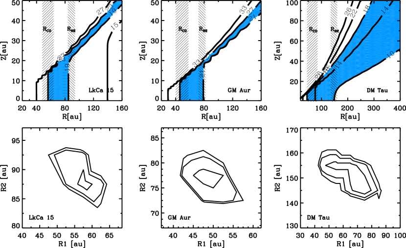
Figure 7: Top panels: CO and N₂ snowlines and and snow-surfaces shown on top of disk temperature profiles. The striped regions show the constraints on the inner and outer N₂H⁺ edges from the jump-and-drop model, interpreted as the CO and N₂ midplane snowline locations. The blue filled regions mark the temperatures between CO and N₂ freeze-out, extracted from a second grid of parametric models. Note the excellent agreement. Lower panels: $\chi^{2}$ surfaces showing model constrains on R1 (inner edge) and R2 (outer edge) in jump-and-drop model for each disk. Contours correspond to the 1–3 $\sigma$ uncertainties.

Table  6 shows the best-fit parameters for R1, R2,J1, D2 and N_p. Figure. 7 shows the $\chi^{2}$ plot and the snowline locations overlapped on the temperature contours of the disks. We find CO snowlines at 48–75 AU and N₂ snowlines at 78–145 AU in the three disks. The derived CO snowlines are consistent with the initial estimates. Figure 8 shows the deprojected profile of the observed N₂H⁺ emission compared with the best-fit models. The best-fit models match the observations very well.

We note that the uncertainties on R1 and R2 of these disks, derived from the $\chi^{2}$ contours, should reflect the sharpness of the ring edges. The uncertainties are typically $\sim 10-40\%$ for R1 and $\sim 5-10\%$ for R2 with respect to the best fit value. Table 6 indicates that the edges on the disks of LkCa 15 and GM Aur are sharper than those of DM Tau. This could relate to a smaller $\epsilon$ for dust settling for DM Tau compared to the other two disks. Observations on a larger sample of disks are needed to confirm whether the sharpness of the edges is correlated with $\epsilon$. Turbulent diffusion in disks might also play an important role on the sharpness of the emission edges (Owen, 2014), which needs to be further explored.

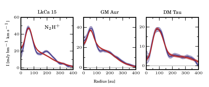
Figure 8: Observed N₂H⁺ $3-2$ profiles vs simulated observations of best-fit models in the jump-and-drop model framework illustrated in Figure. 6.

Based on comparison between R1 and R2, and the disk temperature structures we can derive snowline temperatures for CO and N₂ in the three disks as shown in Table 6. We find CO snowline temperatures of 21–25, 24–28 and 13–18 K, and N₂ snowline temperatures of 18–19, 20–22, and 9–10 K for LkCa 15, GM Aur and DM Tau, respectively. The low values obtained for DM Tau are noteworthy and are discussed further below.

Perhaps simplistically we expect that the same freeze-out and desorption equilibrium that is setting the snowline temperature in the midplane should also set it along the snow surfaces throughout the disk. A complementary model approach to the above ‘Jump-and-drop’ model is then to assume a constant N₂H⁺ abundance between two temperature boundaries corresponding to CO and N₂ freeze-out. To evaluate the robustness of the results obtained from the jump-and-drop model, we therefore ran a second grid of parametric models characterized by the CO freeze-out temperature T_CO, the N₂ freeze-out temperature T${}_{\rm{N_{2}}}$, and the fractional abundance of N₂H⁺. The best-fit T_CO and T${}_{\rm{N_{2}}}$ are 23 and 19 K for LkCa 15, 27 and 21 K for GM Aur, and 18 and 10 K for DM Tau, in perfect agreement with the results obtained from the jump-and-drop models. The locations of these temperature regions are shown by the blue shades in Figure. 7, demonstrating excellent agreement between this set of models and the jump-and-drop models used to establish snowline locations.

4 Discussion

4.1 CO and N₂ freeze-out temperatures

There are two previously derived CO snowline temperatures from N₂H⁺emission modeling: 17 K in the disk of TW Hya, and 25 K in the disk of HD 163295 (Qi et al., 2013, 2015). The low value for TW Hya has been contested, however, and an analysis using CO isotopologues instead resulted in a CO snowline at 27 K (Zhang et al., 2017). In the disk warm molecular layer, the freeze-out termperature of CO is constrainted to be around 21 K toward the TW Hya (Schwarz et al., 2016) and IM Lup (Pinte et al., 2018) disks. Our new CO snowline temperatures of 13–18 K (DM Tau), 21–25 K (LkCa 15), and 24–28 K (GM Aur) add to this list and show that there is a real range of CO snowline temperatures, also among T Tauri disks.

The ranges of observed CO and N₂ snowline temperatures for GM Aur and LkCa 15 compare well with expectations from laboratory experiments (Collings et al., 2004; Öberg et al., 2005; Bisschop et al., 2006; Fayolle et al., 2016). Measured CO binding energies range from 870 K (pure CO ice) to 1300 K (adsorbed onto compact H₂O ice) corresponding to snowline temperatures of $\sim$21–32 K, respectively, assuming a midplane n_H density of 10¹⁰ cm^-3 and a CO abundance of $5\times 10^{-5}$ with respect to n_H. Measured N₂ binding energies range from 770 K to 1140 for analogous ices, corresponding to snowline temperatures of $\sim$18–27 K, respectively, assuming the same midplane n_H density as above, and a N₂ abundance of $3\times 10^{-5}$ with respect to n_H (assuming that 95% of the N atoms are in N₂). The extracted LkCa 15 and GM Aur CO and N₂ snowline temperatures suggest that both volatiles reside on moderately water-rich ice grains, if the disks are effectively static. Pebbles are however subject to radial drift on timescales similar to sublimation, which can move snowlines inwards, to higher disk temperatures than expected (Piso et al., 2015). If drift is important in these disks, or if the disks are a few degrees warmer than modelled, CO and N₂ could be sublimating from close to pure ice layers.

The DM Tau CO and N₂ snowline temperatures are considerably lower than the lowest expected value; the contrast between expected and observed N₂ snowline temperatures is almost a factor of 2! There are possible explanations for such low freeze-out temperatures, including radial mixing, turbulent, vertical mixing (Aikawa, 2007), and photodesorption (Hersant et al., 2009), but all are highly speculative considering the large opacities and low turbulence levels expected in disk midplanes (e.g. Teague et al., 2016; Flaherty et al., 2018). Photodesorption has been previously invoked as an explanation for observations of cold CO gas in the GM Aur, LkCa 15, and DM Tau disks (Dartois et al., 2003; Piétu et al., 2007), and may play a larger role in setting the division of volatiles between gas and grains in the DM Tau disk compared to the other two disks. Another possible explanation is that the disk is actually substantially warmer than the best-fit DIAD model. To distinguish between these different explanations we need direct measurements of the N₂ gas temperatures between the CO and N₂ snowlines. Resolved observations of a second N₂H⁺ transition with a substantial difference in upper energy level from the existing $3-2$ transition, will be essential to provide the model-independent measurements of the temperature range at which CO and N₂ snowlines occur.

Finally it is illustrative to compare the ratios of observed and expected CO and N₂ snowline temperatures. In laboratory experiments the N₂ sublimation energy is consistently 10% lower than the CO sublimation temperature, when considering identical ice environments. Once again the LkCa 15 and GM Aur observations are consistent with expectations – snowline temperature ratios range between 0.7 and 0.9 for both disks – and DM Tau is not. In the latter case the CO/N₂ snowline temperature ratio varies between 0.5 and 0.77. Such low ratios can be achieved in the laboratory if CO sublimation from a water-rich ice is compared with N₂ sublimation from a water-poor ice. Given that the DM Tau temperature profile is correct, the DM Tau results suggest that CO and N₂ sometimes reside in different ice environments in the same disk, where e.g. CO is in a more strongly bound ice, while N₂ is frozen out in a weakly bonding ice layer. There may thus not be a fixed ratio between the CO and N₂ snowline locations in disks. We note, however, that if the adopted temperature profile is off by only two degrees at the N₂ snowline we could not rule out that both CO and N₂ are present in similar, hypervolatile ice environments.

4.2 Snowlines and double-ring dust substructures in disks

Millimeter observations of protoplanetary disks at high angular resolution have revealed a wealth of substructures (e.g. ALMA Partnership et al., 2015; Andrews et al., 2012; Isella et al., 2016; Long et al., 2018; Andrews et al., 2018b). Many of these structures are concentric and axisymmetric, e.g. gaps and rings. The snowlines of major volatile species may play a role in creating these features, through rapid particle growth by condensation (e.g. Ros & Johansen, 2013; Zhang et al., 2015; Pinilla et al., 2017), or aggregate sintering (Okuzumi et al., 2016), or pile-ups of material due to increased fragmentation (Stammler et al., 2017). If the latter mechanism dominates, the increase in surface density around snowlines will be seen as bright rings in millimeter observations. The more abundant the volatile species is, the effect is stronger. Therefore we should expect a double-ring system in the outer disk associated with the CO and N₂ snowlines.

The relationship between snowline locations and disk sub-structure has recently been tested in large samples with 10s of disks. In particular, Long et al. (2018) and Huang et al. (2018) found no obvious correspondence between the locations of the substructures and the disk midplane temperatures, and inferred that major snow lines in mature disks do not play an important role in regulating observed sub-structures. These conclusions rely on two assumptions, however, that disk midplane temperature structures can be well approximated using simple models, and that the same snowlines generally occur at the same disk temperatures. In Section 3 we showed that snowline temperatures can vary by up to a factor of two and this range may in reality be even larger, since we do not account for snowline locations in settled disks. It is difficult to know the temperature structure of a disk in detail, but the chemical structure (i.e. where the N₂H⁺ emission lies) is perhaps a more robust way of isolating the CO and N₂ snowlines.

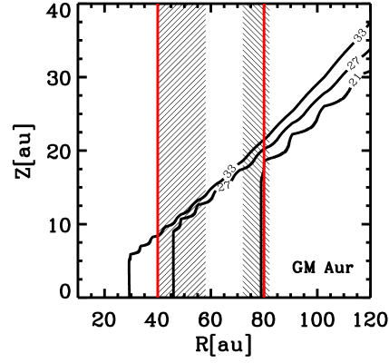
Figure 9: The dust ring locations determined in the GM Aur disk (Macías et al., 2018) in red lines and the constraints on the CO and N₂ snowline locations in striped regions shown on top of its disk temperature profiles in contours.

One of our disks, GM Aur, is observed at high enough resolution to resolve its ringed sub-structure, and in this case we do not need to make assumptions about snowline locations, but can rather test directly whether there is a relationship between snowlines and dust rings. High resolution ($\sim$0.2^′′) observations of dust continuum emission from GM Aur (Macías et al., 2018) revealed two bright rings at 40 and 80 au (Figure. 9), which can be compared to our extracted CO and N₂ snowline locations of 40–58 AU and 74–84 AU, respectively. This coincidence is suggestive, but needs to be tested for more disks. So far, high angular resolution ($\sim$40 mas observations of DM Tau don’t appear to show any double-ring dust structure associated with the CO and N₂ snowline locations (Kudo et al., 2018). However their integrations on source were too short to detect the little “bump” around 100 AU from the azimuthally averaged radial profile in our deprojected image of DM Tau (Figure 2). So long-baseline continuum observations with deep integrations are needed for the DM Tau and LkCa 15 disks to define better their detailed sub-structure. The presence of similar double-ring systems coincident with snowline locations in all disks would provide evidence of a close relationship between snowline locations and dust sub-structure.

Finally we note, that whether a disk has vertical snow surfaces, may affect how much midplane snowlines change the coagulation, fragmentation and sintering efficiencies of pebbles. All existing models assume a vertically isothermal disk and hence vertical snow surfaces (e.g. Okuzumi et al., 2016; Stammler et al., 2017), and flatter snow surfaces may reduce the effect of snowline crossings on grain growth and destruction. It is therefore possible that there are two populations of disks with sub-structures, one where some or all dust rings are caused by snowline-related processes, and a second, settled disk population where snowline locations do not affect the emergence of dust sub-structure.

4.3 Disk temperature structure and uncertainty in gas CO measurements

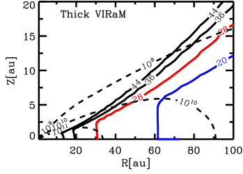
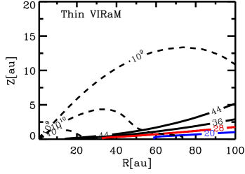
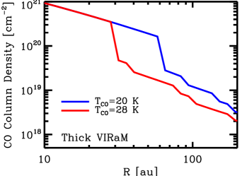
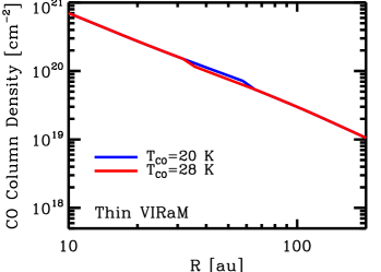
Figure 10: Top panels: Temperature and density profiles of the models with a thick or thin VIRaM layer. Bottom panels: The predicted CO radial column density profiles for both models, assuming T_CO=28 K (red line) and 20 K (blue line).

An additional implication of this work regards the total disk gas mass. The determination of protoplanetary disk masses is fundamental for understanding the formation and evolution of disks and planets. The observation of CO and its isotopologues has been used as a measure of the total disk gas content (e.g. Williams & Best, 2014). However there are many sources of uncertainty in gas mass measurements from CO observations, e.g. chemical sequestration (Bergin et al., 2016) and selective photo-dissociation (Miotello et al., 2016). Here we show an even more fundamental problem of using CO observations to determine the disk gas mass, namely, the diversity of vertical temperature structure among disks, and its impact on CO vertical gas abundance profiles in individual disks.

Detailed modeling of disk SEDs, as shown above, reveal a range of thicknesses for VIRaM layers. The vertical temperature structure regulates the vertical distribution of CO gas and ice and hence the amount of gas-phase CO which can be traced through (optically thin) CO isotopologue observations. We demonstrate the magnitude of this effect in Figure. 10, where we model the distribution of CO in two DIAD models with the same midplane temperatures, but with different vertical temperature profiles (cf. Figure 3). We assume that [¹²CO]/[H₂]=10^-4 where $T>T_{\rm CO}$ and that it is reduced by two orders of magnitude where $T<T_{\rm CO}$, and make predictions for two cases: T_CO=20 and 28 K, corresponding to CO freeze-out on water-poor and water-rich ices, respectively. Figure 10 shows that for each assumed CO freeze-out temperature, disks with and without a thick VIRaM layer present different CO column density radial profiles, both in terms of shapes and absolute column densities. The latter varies by factors of 2–5 between the two disk models. In the model with a thick VIRaM layer, 20% (T_CO=28 K) to 40% (T_CO=20 K) of the available CO is in the gas-phase within 200 AU. By contrast, in the model without such a thick VIRaM layer 90% of the available CO is in the gas interior to 200 AU, regardless of CO freeze-out temperature. Note the subtle drop of the CO column density in this kind of model. In summary, in a disk with a set midplane temperature profile, 20–90% of the total CO resides in the gas-phase. Without detailed disk models it is therefore challenging to accurately account for CO freeze-out when using CO gas lines to estimate disk gas masses. To develop CO emission lines as accurate probes of disk gas mass instead requires high resolution observations of both CO isotopologues and N₂H⁺, which together can be used to constrain the disk vertical structure.

5 Summary

We present high angular resolution N₂H⁺ $3-2$ observations of 6 single-disk systems. These observations show that N₂H⁺ probes both the CO and N₂ snow surfaces. Our findings are as follows:

• We find two distinctive emission morphologies in the N₂H⁺ $3-2$ emission: either in a bright, narrow ring surrounded by extended tenuous emission (LkCa 15, GM Aur, DM Tau) or in a broad ring for most of the emission (V4046 Sgr, AS 209, IM Lup).

• The bright, narrow ring pattern can be explained by N₂H⁺emission tracing vertical snow surfaces of CO and N₂ in disks with a thick VIRaM layer. In these disks, we use the inner and outer edges of the bright N₂H⁺ ring to constrain the first set of CO and N₂ snowline pairs in disks.

• Broad N₂H⁺ rings are found in disks with a thin VIRaM layer, where the N₂ snowline cannot be constrained and only upper limits of the CO snowline locations can be obtained.

• In disks where both CO and N₂ snowlines are located, we can determine the snowline temperatures based on the temperature structures of their respective disk models. The CO and N₂ snowline temperatures in the disks of LkCa 15 and GM Aur are consistent with CO and N₂ freeze-out on moderately water-rich ice grains in an effectively static disk. However, those in the DM Tau disk are considerably lower than the lowest expected value.

Our observations and analysis show that the N₂H⁺ imaging approach has tremendous potential to efficiently constrain the shape of CO and N₂ snow surfaces and the location of the corresponding snowlines. The results reveal a range of N₂ and CO snowline radii towards stars of similar spectra type, which demonstrate the need for empirically determined snowlines in disks.

Appendix A Channel Images

Figures 11- 16 show channel maps for N₂H⁺ $3-2$ emission toward the six disks.

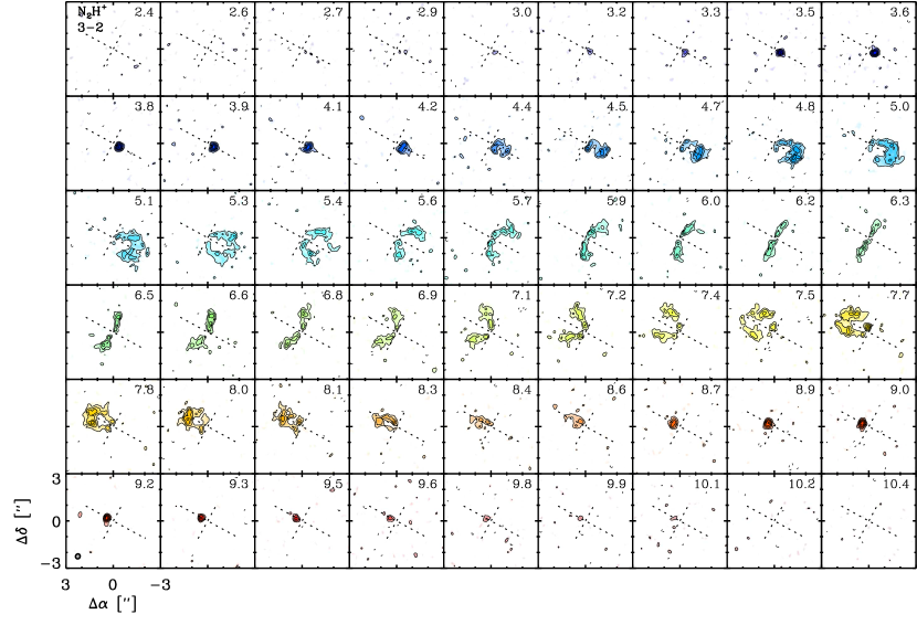
Figure 11: N₂H⁺ $3-2$ channel maps of the LkCa 15 disk. Contours are drawn at [3, 5, 7 …]$\sigma$, where $\sigma$ is the channel rms listed in Table 4. Cross-hatches mark the stellar position and orientation of the disk position angle. The synthesized beam dimensions are drawn in the bottom left panel; LSR velocity (in km s^-1) are marked in the top right of each panel. The offset from the stellar position in arcseconds is marked on the axes in the lower left corner.

Appendix B Hyper-fine components of the N₂H⁺ $3-2$ transition

Table 7 lists the 29 N₂H⁺ hyper-fine components of the $3-2$ transition and the Einstein A coefficients from the CDMS catalog.

Table 7: Hyper-fine components of N₂H⁺ $3-2$

Frequency (GHz)	A (10-4 s-1)
279.5094802	0.1212
279.5098032	1.668
279.5098546	1.572
279.5098764	0.8648
279.5102508	0.1304
279.5111134	2.625
279.5113207	8.162
279.5113628	6.312
279.5113923	0.6818
279.5114098	1.706
279.5114848	11.50
279.5116237	0.3082
279.5116627	10.77
279.5117767	10.39
279.5117843	11.82
279.5117880	12.23
279.5117885	12.84
279.5118309	5.312
279.5118379	13.52
279.5121022	1.264
279.5123006	1.244
279.5138749	0.3675
279.5139475	0.3759
279.5140869	0.01079
279.5142004	1.951
279.5143188	1.713
279.5143851	1.000
279.5145717	0.2215
279.5147106	0.5236

References

- Aikawa (2007) Aikawa, Y. 2007, ApJ, 656, L93
- Aikawa & Nomura (2006) Aikawa, Y., & Nomura, H. 2006, ApJ, 642, 1152
- ALMA Partnership et al. (2015) ALMA Partnership, Brogan, C. L., Pérez, L. M., et al. 2015, ApJ, 808, L3
- Andrews et al. (2018a) Andrews, S. M., Terrell, M., Tripathi, A., et al. 2018a, ApJ, 865, 157
- Andrews et al. (2011) Andrews, S. M., Wilner, D. J., Espaillat, C., et al. 2011, ApJ, 732, 42
- Andrews et al. (2012) Andrews, S. M., Wilner, D. J., Hughes, A. M., et al. 2012, ApJ, 744, 162
- Andrews et al. (2018b) Andrews, S. M., Huang, J., Pérez, L. M., et al. 2018b, ApJ, 869, L41
- Bergin et al. (2002) Bergin, E. A., Alves, J., Huard, T., & Lada, C. J. 2002, ApJ, 570, L101
- Bergin et al. (2016) Bergin, E. A., Du, F., Cleeves, L. I., et al. 2016, ApJ, 831, 101
- Bisschop et al. (2006) Bisschop, S. E., Fraser, H. J., Öberg, K. I., van Dishoeck, E. F., & Schlemmer, S. 2006, A&A, 449, 1297
- Chiang & Youdin (2010) Chiang, E., & Youdin, A. N. 2010, Annual Review of Earth and Planetary Sciences, 38, 493
- Ciesla & Cuzzi (2006) Ciesla, F. J., & Cuzzi, J. N. 2006, Icarus, 181, 178
- Cleeves (2016) Cleeves, L. I. 2016, ApJ, 816, L21
- Collings et al. (2004) Collings, M. P., Anderson, M. A., Chen, R., et al. 2004, MNRAS, 354, 1133
- D’Alessio et al. (2001) D’Alessio, P., Calvet, N., & Hartmann, L. 2001, ApJ, 553, 321
- D’Alessio et al. (2006) D’Alessio, P., Calvet, N., Hartmann, L., Franco-Hernández, R., & Servín, H. 2006, ApJ, 638, 314
- D’Alessio et al. (1999) D’Alessio, P., Calvet, N., Hartmann, L., Lizano, S., & Cantó, J. 1999, ApJ, 527, 893
- D’Alessio et al. (1998) D’Alessio, P., Canto, J., Calvet, N., & Lizano, S. 1998, ApJ, 500, 411
- D’Alessio et al. (2005) D’Alessio, P., Hartmann, L., Calvet, N., et al. 2005, ApJ, 621, 461
- Dartois et al. (2003) Dartois, E., Dutrey, A., & Guilloteau, S. 2003, A&A, 399, 773
- Draine & Lee (1984) Draine, B. T., & Lee, H. M. 1984, ApJ, 285, 89
- Espaillat et al. (2011) Espaillat, C., Furlan, E., D’Alessio, P., et al. 2011, ApJ, 728, 49
- Fayolle et al. (2016) Fayolle, E. C., Balfe, J., Loomis, R., et al. 2016, ApJ, 816, L28
- Fedele et al. (2018) Fedele, D., Tazzari, M., Booth, R., et al. 2018, A&A, 610, A24
- Flaherty et al. (2018) Flaherty, K. M., Hughes, A. M., Teague, R., et al. 2018, ApJ, 856, 117
- Flower (1999) Flower, D. R. 1999, MNRAS, 305, 651
- Gundlach et al. (2011) Gundlach, B., Skorov, Y. V., & Blum, J. 2011, Icarus, 213, 710
- Guzmán et al. (2018) Guzmán, V. V., Huang, J., Andrews, S. M., et al. 2018, ApJ, 869, L48
- Hersant et al. (2009) Hersant, F., Wakelam, V., Dutrey, A., Guilloteau, S., & Herbst, E. 2009, A&A, 493, L49
- Hogerheijde & van der Tak (2000) Hogerheijde, M. R., & van der Tak, F. F. S. 2000, A&A, 362, 697
- Huang et al. (2016) Huang, J., Öberg, K. I., & Andrews, S. M. 2016, ApJ, 823, L18
- Huang et al. (2017) Huang, J., Öberg, K. I., Qi, C., et al. 2017, ApJ, 835, 231
- Huang et al. (2018) Huang, J., Andrews, S. M., Dullemond, C. P., et al. 2018, ApJ, 869, L42
- Hughes et al. (2009) Hughes, A. M., Andrews, S. M., Espaillat, C., et al. 2009, ApJ, 698, 131
- Isella et al. (2016) Isella, A., Guidi, G., Testi, L., et al. 2016, Physical Review Letters, 117, 251101
- Johansen et al. (2007) Johansen, A., Oishi, J. S., Mac Low, M.-M., et al. 2007, Nature, 448, 1022
- Kastner et al. (2018) Kastner, J. H., Qi, C., Dickson-Vandervelde, D. A., et al. 2018, ApJ, 863, 106
- Kudo et al. (2018) Kudo, T., Hashimoto, J., Muto, T., et al. 2018, ApJ, 868, L5
- Long et al. (2018) Long, F., Pinilla, P., Herczeg, G. J., et al. 2018, ApJ, 869, 17
- Macías et al. (2018) Macías, E., Espaillat, C. C., Ribas, Á., et al. 2018, ApJ, 865, 37
- McMullin et al. (2007) McMullin, J. P., Waters, B., Schiebel, D., Young, W., & Golap, K. 2007, in Astronomical Society of the Pacific Conference Series, Vol. 376, Astronomical Data Analysis Software and Systems XVI, ed. R. A. Shaw, F. Hill, & D. J. Bell, 127
- Miotello et al. (2016) Miotello, A., van Dishoeck, E. F., Kama, M., & Bruderer, S. 2016, A&A, 594, A85
- Öberg & Bergin (2016) Öberg, K. I., & Bergin, E. A. 2016, ApJ, 831, L19
- Öberg et al. (2011a) Öberg, K. I., Murray-Clay, R., & Bergin, E. A. 2011a, ApJ, 743, L16
- Öberg et al. (2005) Öberg, K. I., van Broekhuizen, F., Fraser, H. J., et al. 2005, ApJ, 621, L33
- Öberg et al. (2010) Öberg, K. I., Qi, C., Fogel, J. K. J., et al. 2010, ApJ, 720, 480
- Öberg et al. (2011b) —. 2011b, ApJ, 734, 98
- Okuzumi et al. (2016) Okuzumi, S., Momose, M., Sirono, S.-i., Kobayashi, H., & Tanaka, H. 2016, ApJ, 821, 82
- Owen (2014) Owen, J. E. 2014, ApJ, 790, L7
- Piétu et al. (2007) Piétu, V., Dutrey, A., & Guilloteau, S. 2007, A&A, 467, 163
- Pinilla et al. (2017) Pinilla, P., Pohl, A., Stammler, S. M., & Birnstiel, T. 2017, ApJ, 845, 68
- Pinte et al. (2018) Pinte, C., Ménard, F., Duchêne, G., et al. 2018, A&A, 609, A47
- Piso et al. (2015) Piso, A.-M. A., Öberg, K. I., Birnstiel, T., & Murray-Clay, R. A. 2015, ApJ, 815, 109
- Piso et al. (2016) Piso, A.-M. A., Pegues, J., & Öberg, K. I. 2016, ApJ, 833, 203
- Qi et al. (2011) Qi, C., D’Alessio, P., Öberg, K. I., et al. 2011, ApJ, 740, 84
- Qi et al. (2015) Qi, C., Öberg, K. I., Andrews, S. M., et al. 2015, ApJ, 813, 128
- Qi et al. (2013) Qi, C., Öberg, K. I., Wilner, D. J., et al. 2013, Science, 341, 630
- Ros & Johansen (2013) Ros, K., & Johansen, A. 2013, A&A, 552, A137
- Rosenfeld et al. (2013) Rosenfeld, K. A., Andrews, S. M., Wilner, D. J., Kastner, J. H., & McClure, M. K. 2013, ApJ, 775, 136
- Sault et al. (1995) Sault, R. J., Teuben, P. J., & Wright, M. C. H. 1995, in Astronomical Society of the Pacific Conference Series, Vol. 77, Astronomical Data Analysis Software and Systems IV, ed. R. A. Shaw, H. E. Payne, & J. J. E. Hayes, 433
- Schöier et al. (2005) Schöier, F. L., van der Tak, F. F. S., van Dishoeck, E. F., & Black, J. H. 2005, A&A, 432, 369
- Schwarz et al. (2016) Schwarz, K. R., Bergin, E. A., Cleeves, L. I., et al. 2016, ApJ, 823, 91
- Stammler et al. (2017) Stammler, S. M., Birnstiel, T., Panić, O., Dullemond, C. P., & Dominik, C. 2017, A&A, 600, A140
- Teague et al. (2016) Teague, R., Guilloteau, S., Semenov, D., et al. 2016, A&A, 592, A49
- van ’t Hoff et al. (2017) van ’t Hoff, M. L. R., Walsh, C., Kama, M., Facchini, S., & van Dishoeck, E. F. 2017, A&A, 599, A101
- Williams & Best (2014) Williams, J. P., & Best, W. M. J. 2014, ApJ, 788, 59
- Xu et al. (2017) Xu, R., Bai, X.-N., & Öberg, K. 2017, ApJ, 835, 162
- Zhang et al. (2017) Zhang, K., Bergin, E. A., Blake, G. A., Cleeves, L. I., & Schwarz, K. R. 2017, Nature Astronomy, 1, 0130
- Zhang et al. (2015) Zhang, K., Blake, G. A., & Bergin, E. A. 2015, ApJ, 806, L7