Kernel Methods for Surrogate Modeling

Abstract

This chapter deals with kernel methods as a special class of techniques for surrogate modeling. Kernel methods have proven to be efficient in machine learning, pattern recognition and signal analysis due to their flexibility, excellent experimental performance and elegant functional analytic background. These data-based techniques provide so called kernel expansions, i.e., linear combinations of kernel functions which are generated from given input-output point samples that may be arbitrarily scattered. In particular, these techniques are meshless, do not require or depend on a grid, hence are less prone to the curse of dimensionality, even for high-dimensional problems.

In contrast to projection-based model reduction, we do not necessarily assume a high-dimensional model, but a general function that models input-output behavior within some simulation context. This could be some micro-model in a multiscale-simulation, some submodel in a coupled system, some initialization function for solvers, coefficient function in Partial Differential Equations (PDEs), etc.

First, kernel surrogates can be useful if the input-output function is expensive to evaluate, e.g. is a result of a finite element simulation. Here, acceleration can be obtained by sparse kernel expansions. Second, if a function is available only via measurements or a few function evaluation samples, kernel approximation techniques can provide function surrogates that allow global evaluation.

We present some important kernel approximation techniques, which are kernel interpolation, greedy kernel approximation and support vector regression. Pseudo-code is provided for ease of reproducibility. In order to illustrate the main features, commonalities and differences, we compare these techniques on a real-world application. The experiments clearly indicate the enormous acceleration potential.

1 Introduction

This chapter deals with kernel methods as tools to construct surrogate models of arbitrary functions, given a finite set of arbitrary samples.

These methods generate approximants based solely on input-output pairs of the unknown function, without geometrical constraints on the sample locations. In particular, the surrogates do not necessarily depend on the knowledge of an high-dimensional model but only on its observed input-output behavior at the sample sites, and they can be applied on arbitrarily scattered points in high dimension.

These features are particularly useful when these methods are applied within some simulation context. For example, kernel surrogates can be useful if the input-output function is expensive to evaluate, e.g. is a result of a finite element simulation. Here, acceleration can be obtained by sparse kernel expansions. Moreover, if a function is available only via measurements or a few function evaluation samples, kernel approximation techniques can provide function surrogates that allow global evaluation.

Kernel methods are used with much success in Model Order Reduction, and far beyond the scope of this chapter. For example, they have been used in the modeling of geometry transformations and mesh coupling [3, 12, 13], and in mesh repair methods [33], or in the approximation of stability factors and error indicators [32, 34, 14], where only a few samples of the exact indicators are sufficient to construct an efficient surrogate to be used in the online phase. Moreover, kernel methods have been combined with projection based MOR methods, e.g. to obtain simulation-based classification [60], or to derive multi-fidelity Monte Carlo approximations [40]. Kernel surrogates have been employed in optimal control problems [51, 59], in the coupling of multi-scale simulations in biomechanics [69, 25], in real time prediction for parameter identification and state estimation in biomechanical systems [29], in gas transport problems [22], in the reconstruction of potential energy surfaces [30], in the forecasting of time stepping methods [6], in the reduction of nonlinear dynamical systems [67], in uncertainty quantification [28], and for nonlinear balanced truncation of dynamical systems [5].

In further generality, there exists many kernel-based algorithms and application fields that we do not address here. Mainly, we mention the solution of PDEs, in which several approaches have emerged in the last years, and which particularly allow to solve problems with unstructured grids on general geometries, including high dimensional manifolds (see e.g. [17, 11]). Moreover, several other techniques are studied within Machine Learning, such as classification, density estimation, novelty detection or feature extraction (see e.g. [53, 54]).

Furthermore, we remark that these methods are members of the larger class of machine learning and approximation techniques, which are generally suitable to construct models based on samples to make prediction on new inputs. These models are usually referred to as surrogates when they are then used as replacements of the model that generated the data, as they are able to provide an accurate and faster response. Some examples of these techniques are classical approximation methods such as polynomial interpolation, which are used in this context especially in combination with sparse grids to deal with high-dimensional problems (see [19]), and (deep) neural network models. The latter in particular have seen a huge increase in analysis and application in the recent years. For a recent treatment of deep learning, we refer e.g. to [21].

Despite these very diverse applications and methodologies, kernel methods can be analyzed to some extent in the common framework of Reproducing Kernel Hilbert spaces and, although the focus of this chapter will be on the construction of sparse surrogate models, parts of the following discussion can be the starting point for the analysis of other techniques.

In general terms, kernel methods can be viewed as nonlinear versions of linear algorithms. As an example, assume to have some set $X_{n}:=\{x_{k}\}_{k=1}^{n}\subset\mathbb{R}^{d}$ of data points and target data values $Y_{n}:=\{y_{k}\}_{k=1}^{n}\subset\mathbb{R}$. We can construct a surrogate $s:\mathbb{R}^{d}\to\mathbb{R}$ that predicts new data via linear regression, i.e., find $w\in\mathbb{R}^{d}$ s.t. $s(x):=\left\langle w,x\right\rangle$, where $\left\langle\cdot,\cdot\right\rangle$ is the scalar product in $\mathbb{R}^{d}$. A good surrogate model $s$ will give predictions such that $|s(x_{k})-y_{k}|$ is small. If we can write $w\in\mathbb{R}^{d}$ as $w=\sum_{j=1}^{n}\alpha_{j}x_{j}$ for a set of coefficients $\left(\alpha_{i}\right)_{i=1}^{n}\in\mathbb{R}^{n}$, then $s$ can be rewritten as

$$s(x):=\sum_{j=1}^{n}\alpha_{j}\left\langle x_{j},x\right\rangle.$$

Note that this formulation includes also regression with an offset (or bias) $b\neq 0$, which can be written in this form by an extended representation as

$$s(x):=\left\langle w,x\right\rangle+b=:\left\langle\bar{w},\bar{x}\right\rangle,$$

where $\bar{x}:=(x,1)^{T}\in\mathbb{R}^{d+1}$ and $\bar{w}:=(w,b)^{T}\in\mathbb{R}^{d+1}$.

Using now the Gramian matrix $A\in\mathbb{R}^{n\times n}$ with entries $A_{ij}:=\left\langle x_{i},x_{j}\right\rangle$ and rows $A_{i}^{T}\in\mathbb{R}^{n}$, we look for the surrogate $s$ which minimizes

$$\sum_{i=1}^{n}\left(s(x_{i})-y_{i}\right)_{2}^{2}=\sum_{i=1}^{n}\left(A_{i}^{T}\alpha-y_{i}\right)_{2}^{2}=\left\|A\alpha-y\right\|_{2}^{2}.$$

Additionally, a regularization term can be added to keep the norm of $\alpha$ small, e.g. in terms of the value $\alpha^{T}A\alpha$. Thus, the surrogate can be characterized as the solution of the optimization problem

$$\min_{\alpha\in\mathbb{R}^{n}}\left\|A\alpha-y\right\|_{2}^{2}+\lambda\alpha^{T}A\alpha,$$

i.e., $\alpha=(A+\lambda I)^{-1}y$ if $\lambda>0$.

In many cases this (regularized) linear regression is not sufficient to obtain a good surrogate. A possible idea is to try to combine this linear, simple method with a nonlinear function which maps the data to a higher dimensional space, where the hope is that the image of the data can be processed linearly. For this we consider a so-called feature map $\Phi:\mathbb{R}^{d}\to H$, where $H$ is a Hilbert space, and apply the same algorithm to the transformed data $\Phi(X_{n}):=\{\Phi(x_{i})\}_{i=1}^{n}$ with the same values $Y_{n}$. Since the algorithm depends on $X_{n}$ only via the Gramian $A$, it is sufficient to replace it with the new Gramian $A_{ij}:=\left\langle\Phi(x_{i}),\Phi(x_{j})\right\rangle_{H}$ to obtain a nonlinear algorithm.

We will see that $\left\langle\Phi(x),\Phi(y)\right\rangle_{H}$ defines in fact a positive definite kernel, and if any numerical procedure can be written in terms of inner products of the inputs, it can be transformed in the same way into a new nonlinear algorithm simply by replacing the inner products with kernel evaluations (the so-called kernel trick). We will discuss the details of this procedure in the next sections in the case of interpolation and Support Vector Regression, but this immediately gives a glance of the ample spectrum of algorithms in the class of kernel methods.

This chapter is organized as follows. Section 2 covers the basic notions on kernels and kernel-based spaces which are necessary for the development and understanding of the algorithms. The next Section 3 presents the general ideas and tools to construct kernel surrogates as characterized by the Representer Theorem, and these ideas are specialized to the case of kernel interpolation in Section 4 and Support Vector Regression in Section 5. In both cases, we provide the theoretical foundations as well as the algorithmic description of the methods, with particular attention to techniques to enforce sparsity in the model. These surrogates can be used to perform various analyses of the full model, and we give some examples in Section 6. Section 7 presents a general strategy to choose the various parameters defining the model, whose tuning can be critical for a successful application of the algorithms. Finally, we discuss in Section 8 the numerical results of the methods on a real application dataset, comparing training time (offline), prediction time (online), and accuracy.

2 Background on kernels

We start by introducing some general facts of positive definite kernels. Further details on the general analytical theory of reproducing kernels can be found e.g. in the recent monograph [45], while the books [15, 65] and [53, 55] contain a treatment of kernel theory from the point of view of pattern analysis and scattered data interpolation, respectively.

2.1 Positive definite kernels

Given a nonempty set $\Omega$, which can be a subset of $\mathbb{R}^{d}$, $d\in\mathbb{N}$, but also a set of structured objects such as strings or graphs, a real- and scalar-valued kernel $K$ on $\Omega$ is a bivariate symmetric function $K:\Omega\times\Omega\to\mathbb{R}$, i.e., $K(x,y)=K(y,x)$ for all $x,y\in\Omega$. For our purposes, we are interested in (strictly) positive definite kernels, defined as follows.

Definition 1 (Positive definite kernels).

Let $\Omega$ be a nonempty set. A kernel $K$ on $\Omega$ is positive definite (PD) on $\Omega$ if for all $n\in\mathbb{N}$ and for any set of $n$ pairwise distinct elements $X_{n}:=\{x_{i}\}_{i=1}^{n}\subset\Omega$, the kernel matrix (or Gramian matrix) $A:=A_{K,X_{n}}\in\mathbb{R}^{n\times n}$ defined as $A_{ij}:=K(x_{i},x_{j})$, $1\leq i,j\leq n$, is positive semidefinite, i.e., for all vectors $\alpha:=\left(\alpha_{i}\right)_{i=1}^{n}\in\mathbb{R}^{n}$ it holds

$$\alpha^{T}A\alpha=\sum_{i,j=1}^{n}\alpha_{i}\alpha_{j}K(x_{i},x_{j})\geq 0.$$ (1)

The kernel is strictly positive definite (SPD) if the kernel matrix is positive definite, i.e., (1) holds with strict inequality when $\alpha\neq 0$.

The further class of conditionally (strictly) positive definite kernels is also of interest in certain contexts. We refer to [65, Chapter 8] for their extensive treatment, and we just mention that they are defined as above, except that the condition (1) has to be satisfied only for the subset of coefficients $\alpha$ which match a certain orthogonality condition. When this condition is defined with respect to a space of polynomials of degree $m\in\mathbb{N}$, the resulting kernels are used e.g. to guarantee a certain polynomial exactness of the given approximation scheme, and they are often employed in certain methods for the solution of PDEs.

2.2 Examples and construction of kernels

Despite the abstract definition, there are several ways to construct functions $K:\Omega\times\Omega\to\mathbb{R}$ which are (strictly) positive definite kernels, and usually the proper choice of the kernel is a crucial step in the successful application of the method. We list here a general strategy to construct kernels, and some notable examples.

An often used, constructive approach to design a new kernel is via feature maps as follows.

Proposition 2 (Kernels via feature maps).

Let $\Omega$ be a nonempty set. A feature map $\Phi$ is any function $\Phi:\Omega\to H$, where $\left(H,\left\langle\cdot,\cdot\right\rangle_{H}\right)$ is any Hilbert space (the feature space). The function

$$K(x,y):=\left\langle\Phi(x),\Phi(y)\right\rangle_{H}\;\;x,y\in\Omega,$$

is a PD kernel on $\Omega$.

Proof.

$K$ is a PD kernel since it is symmetric and positive definite, because the inner product is bilinear, symmetric and positive definite. ∎

In many cases, $H$ is either $\mathbb{R}^{m}$ with very large $m$ or even an infinite dimensional Hilbert space. The computation of the possibly expensive $m$- or infinite-dimensional inner product can be avoided if a closed form for $K$ can be obtained. This implies a significant reduction of the computational time required to evaluate the kernel and thus to execute any kind of algorithm.

We see now some examples.

Example 3 (Expansion kernels).

The construction comprises finite dimensional linear combinations, i.e., for a set of functions $\{v_{j}\}_{j=1}^{m}:\Omega\to\mathbb{R}$, the function $K(x,y):=\sum_{k=1}^{m}v_{k}(x)v_{k}(y)$ is a positive definite kernel, having a feature map

$$\Phi(x):=\left(v_{1}(x),v_{2}(x),\dots,v_{m}(x)\right)^{T}\in H:=\mathbb{R}^{m}.$$ (2)

This idea can be extended to an infinite number of functions provided $\{v_{j}(x)\}_{j=1}^{\infty}\in H:=\ell_{2}(\mathbb{N})$ uniformly in $\Omega$, and the resulting kernels are called Hilbert-Schmidt or expansion kernels, which can be proven to be even SPD under additional conditions (see [49]). As an example in $d=1$, we mention the Brownian Bridge kernel $K(x,y):=\max(x,y)-xy$, defined with a feature map $v_{j}(x):=\sqrt{2}(j\pi)^{-1}\sin(j\pi x)$ for $j\in\mathbb{N}$, which is SPD on $\Omega:=(0,1)$. We remark that the kernel can be extended to $(0,1)^{d}$ with $d>1$ using a tensor product of one-dimensional kernels.

This feature map representation proves also that $dim(H)=:m<\infty$ means that the kernel is not SPD in general: e.g., if $X_{n}$ contains $n$ pairwise distinct points and $m<n$, then the vectors $\{\Phi(x_{i})\}_{i=1}^{n}$ can not be linearly independent, and thus the kernel matrix is singular.

Example 4 (Kernels for structured data).

Feature maps are also employed to construct positive definite kernels on sets $\Omega$ of structured data, such as sets of strings, graphs, or any other object. For example, the convolution kernels introduced in [20, 26] consider a finite set of features $v_{1}(x),\dots,v_{m}(x)\in\mathbb{R}$ of an object $x\in\Omega$, and define a feature map exactly as in (2).

Example 5 (Polynomial kernels).

For $a\geq 0$, $p\in\mathbb{N}$, $x,y\in\mathbb{R}^{d}$, the polynomial kernel

$$K(x,y):=\left(\left\langle x,y\right\rangle+a\right)^{p}=\left(\sum_{i=1}^{d}x^{(i)}y^{(i)}+a\right)^{p},\;\;x:=\left(x^{(1)},\dots,x^{(d)}\right)^{T},$$ (3)

is PD on any $\Omega\subset\mathbb{R}^{d}$. It is a $d$-variate polynomial of degree $p$, which contains the monomial terms of degrees $j:=\left(j^{(1)},\dots,j^{(d)}\right)\in J$, for a certain set $J\subset\mathbb{N}_{0}^{d}$. If $m:=|J|$, a feature space is $\mathbb{R}^{m}$ with feature map

$$\Phi(x):=\left(\sqrt{a_{1}}x^{j_{1}},\dots,\sqrt{a_{m}}x^{j_{m}}\right)^{T}.$$

for some positive numbers $\{a_{j}\}_{j=1}^{m}$ and monomials $x^{j_{m}}:=\prod_{i=1}^{d}(x^{(i)})^{j_{m}^{(i)}}$.

Observe that using the closed form (3) of the kernel instead of the feature map is very convenient, since we work with $d$-dimensional instead of $m$-dimensional vectors, where possibly $m:=|J|={{d+p}\choose{d}}=\dim(\mathbb{P}_{p}(\mathbb{R}^{d}))\gg d$.

Example 6 (RBF kernels).

For $\Omega\subset\mathbb{R}^{d}$ in many applications the most used kernels are translational invariant kernels, i.e., there exist a function $\phi:\mathbb{R}^{d}\to\mathbb{R}$ with

$$K(x,y):=\phi(x-y),x,y\in\Omega,$$

and in particular radial kernels, i.e., there exist a univariate function $\phi:\mathbb{R}_{\geq 0}\to\mathbb{R}$ with

$$K(x,y):=\phi(\|x-y\|),x,y\in\Omega.$$

A radial kernel, or Radial Basis Function (RBF), is usually defined up to a shape parameter $\gamma>0$ that controls the scale of the kernel via $K(x,y):=\phi(\gamma\|x-y\|)$.

The main example of such kernels is the Gaussian $K(x,y):=e^{-\gamma^{2}\|x-y\|^{2}}$, which is in fact strictly positive definite. An explicit feature map has been computed in [56]: If $\Omega\subset\mathbb{R}^{d}$ is nonempty, a feature map is the function $\Phi_{\gamma}:\Omega\to L_{2}(\mathbb{R}^{d})$ defined by

$$\Phi_{\gamma}(x):=\frac{(2\gamma)^{\frac{d}{2}}}{\pi^{\frac{d}{4}}}\exp\left(-2\gamma^{2}\|x-\cdot\|^{2}\right),\;\;x\in\Omega.$$

In this case it is even more evident how working with the closed form of $K$ is much more efficient than working with a feature map and computing $L_{2}$-inner products.

RBF kernels offer a significant easiness of implementation in arbitrary space dimension $d$. The evaluation of the kernel $K(\cdot,x)$, $x\in\mathbb{R}^{d}$, on a vector of $n$ points can indeed by realized by first computing a distance vector $D\in\mathbb{R}^{n}$, $D_{i}:=\|x-x_{i}\|$, and then applying the univariate function $\phi$ on $D$. A discussion and comparison of different algorithms (in Matlab) to efficiently compute a distance matrix can be found in [15, Chapter 4], and most scientific computing languages comprise a built-in implementation (such as pdist2 in Matlab and distance_matrix in Scipy).

Translational invariant and RBF kernels can be often analyzed in terms of their Fourier transforms, which provide proofs of their strict positive definiteness via the Bochner Theorem (see e.g. [65, Chapter 6]), and connections to certain Sobolev spaces, as we will briefly see in Section 2.3.

Among various RBF kernels, there are also compactly supported kernels, i.e., $K(x,y)=0$ if $\|x-y\|>1/\gamma$, which produce sparse kernel matrices if $\gamma$ is large enough. The most used ones are the Wendland kernels introduced in [63], which are even radial polynomial within their support.

There are, in addition, various operations to combine positive definite kernels and obtain new ones. For example, sums and products of positive definite kernels and multiplication by a positive constant $a>0$ produce again positive definite kernels. Moreover, if $K^{\prime}$ is a positive definite kernel and $K^{\prime\prime}$ is symmetric with $K^{\prime}\preccurlyeq K^{\prime\prime}$ (i.e., $K:=K^{\prime\prime}-K^{\prime}$ is PD) then also $K^{\prime\prime}$ is positive definite. Furthermore, if $\Omega=\Omega^{\prime}\times\Omega^{\prime\prime}$ and $K^{\prime}$, $K^{\prime\prime}$ are PD kernels on $\Omega^{\prime}$, $\Omega^{\prime\prime}$, then $K(x,y):=K^{\prime}(x^{\prime},y^{\prime})K^{\prime\prime}(x^{\prime\prime},y^{\prime\prime})$ and $K(x,y):=K^{\prime}(x^{\prime},y^{\prime})+K^{\prime\prime}(x^{\prime\prime},y^{\prime\prime})$ are also PD kernels on $\Omega$, i.e., kernels can be defined to respect tensor product structures of the input.

Further details and examples can be found in [45, Chapters 1–2].

2.3 Kernels and Hilbert spaces

Most of the analysis of kernel-based methods is possible through the connection with certain Hilbert spaces. We first give the following definition.

Definition 7 (Reproducing Kernel Hilbert Space).

Let $\Omega$ be a nonempty set, $\mathcal{H}$ an Hilbert space of functions $f:\Omega\to\mathbb{R}$ with inner product $\left\langle\cdot,\cdot\right\rangle_{\mathcal{H}}$. Then $\mathcal{H}$ is called a Reproducing Kernel Hilbert Space (RKHS) on $\Omega$ if there exists a function $K:\Omega\times\Omega\to\mathbb{R}$ (the reproducing kernel) such that

1. $K(\cdot,x)\in\mathcal{H}$ for all $x\in\Omega$,

2. $\left\langle f,K(\cdot,x)\right\rangle_{\mathcal{H}}=f(x)$ for all $x\in\Omega$, $f\in\mathcal{H}$ (reproducing property).

The reproducing property is equivalent to state that, for $x\in\Omega$, the $x$-translate $K(\cdot,x)$ of the kernel is the Riesz representer of the evaluation functional $\delta_{x}:\mathcal{H}\to\mathbb{R}$, $\delta_{x}(f):=f(x)$ for $f\in\mathcal{H}$ , that is hence a continuous functional in $\mathcal{H}$. Also the converse holds, and the following result gives an abstract criterion to check if a Hilbert space is a RKHS.

Theorem 8.

An Hilbert space of functions $\Omega\to\mathbb{R}$ is a RKHS if and only if the point evaluation functionals are continuous in $\mathcal{H}$ for all $x\in\Omega$, i.e., $\delta_{x}\in\mathcal{H}^{\prime}$, the dual space of $\mathcal{H}$. Moreover, the reproducing kernel $K$ of $\mathcal{H}$ is strictly positive definite if and only if the functionals $\{\delta_{x}:x\in\Omega\}$ are linearly independent in $\mathcal{H}^{\prime}$.

Proof.

The first part is clear from the reproducing property, while strict positive definiteness can be checked by verifying that the quadratic form in Definition 1 can not be zero for $\alpha\neq 0$ if $\{\delta_{x}:x\in\Omega\}$ are linearly independent. ∎

We see two concrete examples.

Example 9 (Finite dimensional spaces).

Any finite dimensional Hilbert space $\mathcal{H}$ of functions on a nonempty set $\Omega$ is a RKHS. If $m:=\dim(\mathcal{H})$ and $\{v_{j}\}_{j=1}^{m}$ is an orthonormal basis, then a reproducing kernel is given by

$$K(x,y):=\sum_{j=1}^{m}v_{j}(x)v_{j}(y),\;x,y\in\Omega.$$

Indeed, the two properties of Definition 7 can be easily verified by direct computation.

Example 10 (The Sobolev space $H_{0}^{1}(0,1)$).

The Sobolev space $H_{0}^{1}(0,1)$ with inner product $\left\langle f,g\right\rangle_{H_{0}^{1}}:=\int_{0}^{1}f^{\prime}(y)g^{\prime}(y)dy$ is a RKHS with the Brownian Bridge kernel

$$K(x,y):=\min(x,y)-xy,\;\;x,y\in(0,1)$$

as reproducing kernel (see e.g. [8]). Indeed, $K(\cdot,x)\in H_{0}^{1}(0,1)$, and the reproducing property (2) follows by explicitly computing the inner product.

The following result proves that reproducing kernels are in fact positive definite kernels in the sense of Definition 1. Moreover, the first two properties are useful to deal with the various type of approximants of Section 4 and Section 5, which will be exactly of this form.

Proposition 11.

Let $\mathcal{H}$ be a RKHS on $\Omega$ with reproducing kernel $K$. Let $n,n^{\prime}\in\mathbb{N}$, $\alpha\in\mathbb{R}^{n}$, $\alpha^{\prime}\in\mathbb{R}^{n^{\prime}}$, $X_{n},X_{n^{\prime}}^{\prime}\subset\Omega$, and define the functions

$$f(x):=\sum_{i=1}^{n}\alpha_{i}K(x,x_{i}),\;\;g(x):=\sum_{j=1}^{n^{\prime}}\alpha_{j}^{\prime}K(x,x_{j}^{\prime}),\;\;x\in\Omega.$$

Then we have the following:

1. $f,g\in\mathcal{H}$,

2. $\left\langle f,g\right\rangle_{\mathcal{H}}=\sum_{i=1}^{n}\sum_{j=1}^{n^{\prime}}\alpha_{i}\alpha_{j}^{\prime}K(x_{i},x_{j}^{\prime})$.

3. $K$ is the unique reproducing kernel of $\mathcal{H}$ and it is a positive definite kernel.

Proof.

The first two properties follow from Definition 7, and in particular from $\mathcal{H}$ being a linear space and from the bilinearity of $\left\langle\cdot,\cdot\right\rangle_{\mathcal{H}}$.

For Property (3), the fact that $K$ is symmetric and positive definite, hence a PD kernel, follows from Property (1) of Definition 7, and from the symmetry and positive definiteness of the inner product. Moreover, the reproducing property implies that, if $K,K^{\prime}$ are two reproducing kernels of $\mathcal{H}$, then for all $x,y\in\Omega$ it holds

$$K(x,y)=\left\langle K(\cdot,y),K^{\prime}(\cdot,x)\right\rangle_{\mathcal{H}}=K^{\prime}(x,y).$$

∎

It is common in applications to follow instead the opposite path, i.e., to start with a given PD kernel, and try to see if an appropriate RKHS exists. This is in fact always the case, as proven by the following fundamental theorem from [2].

Theorem 12 (RKHS from kernels – Moore-Aronszajn Theorem).

Let $\Omega$ be a nonempty set and $K:\Omega\times\Omega\to\mathbb{R}$ a positive definite kernel. Then there exists a unique RKHS $\mathcal{H}:=\mathcal{H}_{K}(\Omega)$ with reproducing kernel $K$.

Proof.

The theorem was first proven in [2], to which we refer for a detailed proof. The idea is to deduce that, by Property (1) of Proposition 3, a candidate RKHS $\mathcal{H}$ of $K$ needs to contain the linear space

$$\mathcal{H}_{0}:=\mbox{ span }\{K(\cdot,x):x\in\Omega\}$$

of finite linear combinations of kernel translates. Moreover, from Property (2) of Proposition 11, the inner product on this $\mathcal{H}_{0}$ needs to satisfy

$$\left\langle f,g\right\rangle_{\mathcal{H}} =\sum_{i=1}^{n}\sum_{j=1}^{n^{\prime}}\alpha_{i}\alpha_{j}^{\prime}K(x_{i},x_{j}^{\prime}).$$ (4)

With this observation in mind, the idea of the construction of $\mathcal{H}$ is to start by $\mathcal{H}_{0}$, prove that (4) defines indeed an inner product on $\mathcal{H}_{0}$, and that the completion of $\mathcal{H}_{0}$ w.r.t. this inner product is a RKHS having $K$ as reproducing kernel. Uniqueness then follows from Property (3) of the same proposition. ∎

As it is common in the approximation literature, we will sometimes refer to this unique $\mathcal{H}$ as the native space of the kernel $K$ on $\Omega$.

Remark 13 (Kernel feature map).

Among other consequences, this construction allows to prove that any PD kernel is generated by at least one feature map. Indeed, the function $\Phi:\Omega\to\mathcal{H}$, $\Phi(x):=K(\cdot,x)$, is clearly a feature map for $K$ with feature space $\mathcal{H}$, since the reproducing property implies that

$$\left\langle\Phi(x),\Phi(y)\right\rangle_{H}=\left\langle K(\cdot,x),K(\cdot,y)\right\rangle_{\mathcal{H}}=K(x,y)\;\;\hbox{ for all }x,y\in\Omega.$$

Remark 14.

For certain translational invariant kernels it is possible to prove that the associated native space is norm equivalent to a Sobolev spaces of the appropriate smoothness, which is related to the kernels’ smoothness (see [65, Chapter 10]). This is particularly interesting since the approximation properties of the different algorithms, including certain optimality that we will see in the next sections, are in fact optimal in these Sobolev spaces (with an equivalent norm).

The various operations on positive definite kernels mentioned in Section 2.2 have an analogous effect on the corresponding native spaces. For example, the scaling by a positive number $a>0$ does not change the native space, but scales the inner product correspondingly, and, if $K^{\prime}\preccurlyeq K^{\prime\prime}$ are positive definite kernels, then ${\mathcal{H}}_{K^{\prime}}(\Omega)\subset{\mathcal{H}}_{K^{\prime\prime}}(\Omega)$. We remark that the latter property has been used for example in [71] to prove inclusion relations for the native spaces of RBF kernels with different shape parameters.

2.4 Kernels for vector-valued functions

So far we only dealt with scalar-valued kernels, which are suitable to treat scalar-valued functions. Nevertheless, it is clear that the interest in model reduction is typically also on vector-valued or multi-output functions, which thus require a generalization of the theory presented so far. This has been done in [35], and it is based on the following definition of matrix-valued kernels.

Definition 15 (Matrix-valued PD kernels).

Let $\Omega$ be a nonempty set and $q\in\mathbb{N}$. A function $K:\Omega\times\Omega\to\mathbb{R}^{q\times q}$ is a matrix valued kernel if it is symmetric, i.e., $K(x,y)=K(y,x)^{T}$ for all $x,y\in\Omega$. It is a PD (resp., SPD) matrix-valued kernel if the kernel matrix $A\in\mathbb{R}^{nq\times nq}$ is positive semidefinite (resp., positive definite) for all $n\in\mathbb{N}$ and for all sets $X_{n}\subset\Omega$ of pairwise distinct elements.

This more general class of kernels is also associated to a uniquely defined native space of vector-valued functions, where the notion of RKHS is replaced by the following.

Definition 16 (RKHS for matrix-valued kernels).

Let $\Omega$ be a nonempty set, $q\in\mathbb{N}$, $\mathcal{H}$ an Hilbert space of functions $f:\Omega\to\mathbb{R}^{q}$ with inner product $\left\langle\cdot,\cdot\right\rangle_{\mathcal{H}}$. Then $\mathcal{H}$ is called a vector-valued RKHS on $\Omega$ if there exists a function $K:\Omega\times\Omega\to\mathbb{R}^{q\times q}$ (the matrix-valued reproducing kernel) such that

1. $K(\cdot,x)v\in\mathcal{H}$ for all $x\in\Omega$, $v\in\mathbb{R}^{q}$,

2. $\left\langle f,K(\cdot,x)v\right\rangle_{\mathcal{H}}=f(x)^{T}v$ for all $x\in\Omega$, $v\in\mathbb{R}^{q}$, $f\in\mathcal{H}$ (directional reproducing property).

A particularly simple version of this construction can be realized by considering separable matrix-valued kernels (see e.g. [1]), i.e., kernels that are defined as $K(x,y):=\tilde{K}(x,y)B$, where $\tilde{K}$ is a standard scalar-valued PD kernel, and $B\in\mathbb{R}^{q\times q}$ is a positive semidefinite matrix. In the special case $Q=I$ (the $q\times q$ identity matrix), in [70] it is shown that the native space of $K$ is the tensor product of $q$ copies of the native space of $\tilde{K}$, i.e.,

$$\mathcal{H}_{K}(\Omega)=\left\{f:\Omega\to\mathbb{R}^{q}:f_{j}\in\mathcal{H}_{\tilde{K}}(\Omega),1\leq j\leq q\right\}$$

with

$$\left\langle f,g\right\rangle_{\mathcal{H}_{K}}=\sum_{j=1}^{q}\left\langle f_{j},g_{j}\right\rangle_{\mathcal{H}_{\tilde{K}}}.$$

This simplification will give convenient advantages when implementing some of the methods discussed in Section 4.

3 Data based surrogates

We can now introduce in general terms the two surrogate modeling techniques that we will discuss, namely (regularized) kernel interpolation and Support Vector Regression (SVR).

For both of them, the idea is to represent the expensive map to be reduced as a function $f:\Omega\to\mathbb{R}^{q}$ that maps an input $x\in\Omega$ to an output $y\in\mathbb{R}^{q}$. Here $f$ is assumed to be only continuous, and the set $\Omega$ can be arbitrary as long as a positive definite kernel $K$ can be defined on it. Moreover, the function does not need to be known in any particular way except than through its evaluations on a finite set $X_{n}:=\{x_{k}\}_{k=1}^{n}\subset\Omega$ of pairwise distinct data points, resulting in data values $Y_{n}:=\{y_{k}:=f(x_{k})\}_{k=1}^{n}\subset\mathbb{R}^{q}$.

The goal is to construct a function $s\in\mathcal{H}$ such that $s(x)$ is a good approximation of $f(x)$ for all $x\in\Omega$ (and not only for $x\in X_{n}$), while being significantly faster to evaluate. The process of computing $s$ from the data $(X_{n},Y_{n})$ is often referred to as training of the surrogate $s$, and the set $(X_{n},Y_{n})$ is thus called training dataset.

The computation of the particular surrogate is realized as the solution of an infinite dimensional optimization problem. In general terms, we define a loss function

$$L:\mathcal{H}\times\Omega^{n}\times\left(\mathbb{R}^{q}\right)^{n}\to\mathbb{R}_{\geq 0}\cup\{+\infty\},$$

which takes as input a candidate surrogate $g\in\mathcal{H}$ and the values $X_{n}\in\Omega^{n}$, $Y_{n}\in\left(\mathbb{R}^{q}\right)^{n}$, and returns a measure of the data-accuracy of $g$. Then, the surrogate $s$ is defined as a minimizer, if it exists, of the cost function

$$J(g):=L(g,X_{n},Y_{n})+\lambda\|g\|_{\mathcal{H}}^{2},$$

where the second part of $J$ is a regularization term that penalizes solutions with large norm. The tradeoff between the data-accuracy term and the regularization term is controlled by the regularization parameter $\lambda\geq 0$.

For the sake of presentation, we restrict in the remaining of this section to the case of scalar-valued functions, i.e., $q=1$. The general case follows by using matrix valued kernels as introduced in Section 2.4, and the corresponding definition of orthogonal projections.

The following fundamental Representer Theorem characterizes exactly some solutions of this problem, and it proves that the surrogate will be a function

$$s\in V(X_{n}):=\mbox{ span }\{K(\cdot,x_{i}),x_{i}\in X_{n}\}$$

i.e., a finite linear combination of kernel translates on the training points. A first version of this result was proven in [27], while we refer to [52] for a more general statement.

Theorem 17 (Representer Theorem).

Let $\Omega$ be a nonempty set, $K$ a PD kernel on $\Omega$, $\lambda>0$ a regularization parameter, and let $(X_{n},Y_{n})$ be a training set. Assume that $L(s,X_{n},Y_{n})$ depends on $s$ only via the values $s(x_{i})$, $x_{i}\in X_{n}$.

Then, if the optimization problem

$$\operatorname*{arg\min}_{g\in\mathcal{H}}J(g):=L(g,X_{n},Y_{n})+\lambda\|g\|_{\mathcal{H}}^{2}$$ (5)

has a solution, it has in particular a solution of the form

$$s(x):=\sum_{j=1}^{n}\alpha_{j}K(x,x_{j}),\;\;x\in\Omega,$$ (6)

for suitable coefficients $\alpha\in\mathbb{R}^{n}$.

Proof.

We prove that for every $g\in\mathcal{H}$ there exists $s\in V(X_{n})$ such that $J(s)\leq J(g)$. To see this, we decompose $g\in\mathcal{H}$ as

$$g=s+s^{\perp},\;s\in V(X_{n}),\ s^{\perp}\in V(X_{n})^{\perp}.$$

In particular, since $K(\cdot,x_{i})\in V(X_{n})$, we have by the reproducing property of the kernel that

$$s^{\perp}(x_{i})=\left\langle s,K(\cdot,x_{i})\right\rangle_{\mathcal{H}}=0,\;\;1\leq i\leq n,$$

thus $g(x_{i})=s(x_{i})+s^{\perp}(x_{i})=s(x_{i})$ for $1\leq i\leq n$, and it follows that $L(g,X_{n},Y_{n})=L(s,X_{n},Y_{n})$. Moreover, again by orthogonal projection we have $\|g\|_{\mathcal{H}}^{2}=\|s\|_{\mathcal{H}}^{2}+\|s^{\perp}\|_{\mathcal{H}}^{2}$. Since $\lambda\geq 0$, we then obtain

$$J(s) =L(s,X_{n},Y_{n})+\lambda\|s\|_{\mathcal{H}}^{2}=L(g,X_{n},Y_{n})+\lambda\|s\|_{\mathcal{H}}^{2}$$

$$=L(g,X_{n},Y_{n})+\lambda\|g\|_{\mathcal{H}}^{2}-\lambda\|s^{\perp}\|_{\mathcal{H}}^{2}=J(g)-\lambda\|s^{\perp}\|_{\mathcal{H}}^{2}\leq J(g).$$

Thus, if $g\in\mathcal{H}$ is a solution then $s\in V(X_{n})$ is also a solution. ∎

The existence of a solution will be guaranteed by choosing a convex cost function $J$, i.e., since the regularization term is always convex, by choosing a convex loss function. Then the theorem states that solutions of the infinite dimensional optimization problem can be computed by solving a finite dimensional convex one.

This is a great result, but observe that the evaluation of $s(x)$, $x\in\Omega$, requires the evaluation of the $n$-terms linear combination (6), where $n$ is the size of the dataset. Assuming that the kernel can be evaluated in constant time, the complexity of this operation is $\mathcal{O}(n)$. Thus, to achieve the promised speedup in evaluating the surrogate in place of the function $f$, we will consider in the following methods that enforce sparsity in $s$, i.e., which compute approximate solution where most of the coefficients $\alpha_{j}$ are zero. If the nonzero coefficients correspond to an index set $I_{N}:=\{i_{1},\dots,i_{N}\}\subset\{1,\dots,n\}$, the complexity is reduced to $\mathcal{O}(N)$.

Taking into account this sparsity and denoting $X_{N}:=\{x_{i}\in X_{n}:i\in I_{N}\}$ and $\alpha:=\left(\alpha_{i}:i\in I_{N}\right)$, we can summarize in Algorithm 1 the online phase for any of the following algorithms, consisting in the evaluation of $s$ on a set of points $X_{te}\subset\Omega$. Here and in the following, we denote as $s(X):=(s(x_{1}),\dots,s(x_{m}))^{T}\in\mathbb{R}^{m}$ the vector of evaluations of $s$ on a set of points $X:=\{x_{i}\}_{i=1}^{m}\subset\Omega$.

Algorithm 1 Kernel surrogate - Online phase

1:Input: $X_{N}\in\Omega^{N},\alpha\in\mathbb{R}^{N}$, kernel $K$ (and kernel parameters), test points $X_{te}:=\{x^{te}_{i}\}_{i=1}^{n_{te}}\in\Omega^{n_{te}}$

2:Compute the kernel matrix $A_{te}\in\mathbb{R}^{n_{te}\times N}$, $(A_{te})_{ij}:=K(x^{te}_{i},x_{i_{j}})$.

3:Evaluate the surrogate $s(X^{te})=A_{te}\alpha$.

4:Output: evaluation of the surrogate $s(X^{te})\in\mathbb{R}^{n_{te}}$.

Remark 18 (Normalization of the cost function).

It is sometimes convenient to weight the loss term in the cost function (5) by a factor $1/n$, which normalizes its value with respect to the number of data. We do not use this convention here, and we only remark that this is equivalent to the use of a regularization parameter $\lambda=n\lambda^{\prime}$ for a given $\lambda^{\prime}>0$.

4 Kernel interpolation

The first method that we discuss is (regularized) kernel interpolation. In this case, we consider the square loss function

$$L(s,X_{n},Y_{n}):=\sum_{i=1}^{n}\left(s(x_{i})-y_{i}\right)^{2},$$

which measures the pointwise distance between the surrogate and the target data. We have then the following special case of the Representer Theorem. We denote as $y\in\mathbb{R}^{n}$ the vector of output data, assuming again for now that $q=1$.

Corollary 19 (Regularized interpolant).

Let $\Omega$ be a nonempty set, $K$ a PD kernel on $\Omega$, $\lambda\geq 0$ a regularization parameter. For any training set $(X_{n},Y_{n})$ there exists an approximant of the form

$$s(x)=\sum_{j=1}^{n}\alpha_{j}K(x,x_{j}),\;\;x\in\Omega,$$ (7)

where the vector of coefficients $\alpha\in\mathbb{R}^{n}$ is a solution of the linear system

$$(A+\lambda I)\alpha=y,$$ (8)

where $A\in\mathbb{R}^{n\times n}$, $A_{ij}:=K(x_{i},x_{j})$, is the kernel matrix on $X_{n}$. Moreover, if $K$ is SPD this is the unique solution of the minimization problem (5).

Proof.

The loss $L$ is clearly convex, so there exists a solution of the optimization problem, and by Theorem 17 we know that we can restrict to solutions in $V(X_{n})$.

We then consider functions $s:=\sum_{j=1}^{n}\alpha_{j}K(\cdot,x_{j})$ for some unknown $\alpha\in\mathbb{R}^{n}$. Computing the inner product as in Proposition 11, we obtain

$$s(x_{i})=\sum_{j=1}^{n}\alpha_{j}K(x_{i},x_{j})=(A\alpha)_{i},\;\;\|s\|_{\mathcal{H}}^{2}=\sum_{i,j=1}^{n}\alpha_{i}\alpha_{j}K(x_{i},x_{j})=\alpha^{T}A\alpha.$$

The functional $J$ restricted to $V(X_{n})$ can be parametrized by $\alpha\in\mathbb{R}^{n}$, and thus it can be rewritten as $\tilde{J}:\mathbb{R}^{n}\to\mathbb{R}$ with

$$\tilde{J}(\alpha) =\|A\alpha-y\|_{2}^{2}+\lambda\alpha^{T}A\alpha=(A\alpha-y)^{T}(A\alpha-y)+\lambda\alpha^{T}A\alpha$$

$$=\alpha^{T}A^{T}A\alpha-2\alpha^{T}A^{T}y+y^{T}y+\lambda\alpha^{T}A\alpha,$$

which is convex in $\alpha$ since $A$ is positive semidefinite. Since $A$ is symmetric, its gradient is

$$\nabla_{\alpha}\tilde{J}(\alpha) =2A^{T}A\alpha-2A^{T}y+2\lambda A\alpha=2A(A\alpha-y+\lambda\alpha),$$

i.e., $\nabla_{\alpha}\tilde{J}(\alpha)=0$ if and only if $A\left(A+\lambda I\right)\alpha=Ay$, which is satisfied by $\alpha$ such that $\left(A+\lambda I\right)\alpha=y$. If $K$ is SPD then both $A$ and $A+\lambda I$ are invertible, so this is the only solution. ∎

The extension to vector valued functions, i.e. $q>1$, is straightforward using the separable matrix valued kernels with $B=I$ of Section 2.4. Indeed, in this case the data values are vectors $y_{i}:=f(x_{i})\in\mathbb{R}^{q}$, and thus in the interpolant (7) also the coefficients are vectors $\alpha_{j}\in\mathbb{R}^{q}$. The linear system (8) has the same matrix, but instead $\alpha,y\in\mathbb{R}^{n\times q}$ are defined as

$$\alpha:=\left(\alpha_{1},\dots,\alpha_{n}\right)^{T},\;\;y:=\left(y_{1},\dots,y_{n}\right)^{T}.$$ (9)

We remark that in the following the values $x_{i}$, $y_{i}$, $s(x)$, and $\alpha_{k}$ have always to be understood as row vectors when $q>1$. This notation is very convenient when representing the coefficients as the solution of a linear system. Furthermore, the representation of the dataset samples $(x,y)$ is quite natural when dealing with tabular data, where each column represents a feature and each row a sample vector.

For $K$ SPD and pairwise distinct sample locations $X_{n}$ we can also set $\lambda:=0$ and obtain pure interpolation, i.e., the solution satisfies $L(s,X_{n},Y_{n})=0$, or

$$s(x_{i})=y_{i},\;\;1\leq i\leq n.$$

Observe that this means that with this method we can exactly interpolate arbitrary continuous functions on arbitrary pairwise distinct scattered data in any dimension, as opposite to many other techniques which require complicated conditions on the interpolation points or a grid structure. Moreover, this approximation process has several optimality properties in $\mathcal{H}$, which remind of similar properties of spline interpolation.

Proposition 20 (Optimality of kernel interpolation).

Let $K$ be SPD, $f\in\mathcal{H}$, and $\lambda=0$. Then $s$ is the orthogonal projection of $f$ in $V(X_{n})$, and in particular

$$\|f-s\|_{\mathcal{H}}=\min_{g\in V(X_{n})}\|f-g\|_{\mathcal{H}}.$$

Moreover, if $S:=\left\{g\in\mathcal{H}:g(x_{i})=f(x_{i}),1\leq i\leq n\right\}$, then

$$\left\|s\right\|_{\mathcal{H}}=\min_{g\in S}\|g\|_{\mathcal{H}},$$

i.e., $s$ is the minimal norm interpolant of $f$ on $X_{n}$.

Proof.

The proof is analogous to the proof of the Representer Theorem, using a decomposition $f=g+g^{\perp}$, and proving that $s=g$. ∎

We will see in Section 7 a general technique to tune $\lambda$ using the data, which should return $\lambda=0$ (or very small) when this is the best option. Nevertheless, also for an SPD kernel there are at least two reasons to still consider regularized interpolation. First, the data can be affected by noise, and thus an exact pointwise recovery does not make much sense. Second, a positive parameter $\lambda>0$ improves the condition number of the linear system, and thus the stability of the solution. Indeed, the $2$-condition number of $A+\lambda I$ is

$$\kappa(\lambda):=\frac{\lambda_{\max}(A+\lambda I)}{\lambda_{\min}(A+\lambda I)}=\frac{\lambda_{\max}(A)+\lambda}{\lambda_{\min}(A)+\lambda},$$

which is a strictly decreasing function of $\lambda$, with $\kappa(0)=\kappa(A)$ and $\lim\limits_{\lambda\to\infty}\kappa(\lambda)=1$. Moreover (see [66]) this increased stability can be achieved by still controlling the pointwise accuracy. Namely, if $f\in\mathcal{H}$, it holds

$$\left\|y_{i}-s(x_{i})\right\|_{2}\leq\sqrt{\lambda}\|f\|_{\mathcal{H}}\;\;1\leq i\leq n.$$

We can then summarize the offline phase for regularized kernel interpolation in Algorithm 2.

Algorithm 2 Regularized Kernel interpolation - Offline phase

1:Input: training set $X_{n}\in\Omega^{n}$, $Y_{n}\in\left(\mathbb{R}^{q}\right)^{n}$, kernel $K$ (and kernel parameters), regularization parameter $\lambda\geq 0$.

2:Compute the kernel matrix $A\in\mathbb{R}^{n\times n}$, $A_{ij}:=K(x_{i},x_{j})$.

3:Solve the linear system $(A+\lambda I)\alpha=y$.

4:Output: coefficients $\alpha\in\mathbb{R}^{n\times q}$.

Remark 21 (Flat limit).

The matrix $A$ can be seriously ill-conditioned for certain kernels, and this constitutes a problem at least in the case of pure interpolation. It can also be proven that kernels which guarantee a faster error convergence result in a worse conditioned matrix [48].

For RBF kernels, this happens especially for $\gamma\to 0$ (the so called flat limit), and it is usually not a good idea to directly solve the linear system. In the last years there has been very active research to compute $s$ via different formulations, which rely on different representations of the kernel. We mention here mainly the RBF-QR algorithm [31, 18] and the Hilbert-Schmidt SVD [16] . Both methods are limited so far to only some kernels, but they manage to achieve a great accuracy, which is usually impossible to obtain with the direct solution of the linear system.

Remark 22 (Error estimation).

For SPD translational invariant kernels there is a very detailed error analysis of the interpolation process ($\lambda=0$), for which we refer to [65, Chapter 11]. We only mention that these error bounds assume that $f\in\mathcal{H}$, and are of the form

$$\left\|f-s\right\|_{L_{\infty}(\Omega)}\leq Ch_{n}^{p}\|f\|_{\mathcal{H}},$$

where $C>0$ is a constant independent of $f$, and $h_{n}$ is the fill distance of $X_{n}$ in $\Omega$, i.e.,

$$h_{n}:=h_{X_{n},\Omega}:=\sup\limits_{x\in\Omega}\min\limits_{x_{j}\in X_{n}}\|x-x_{j}\|,$$

which is the analogue of the mesh width for scattered data. Moreover, the order of convergence $p>0$ is dependent on the smoothness of the kernel. In particular, these error bounds can be proven to be optimal when the native space of $K$ is a Sobolev space.

Moreover, these results have been recently extended to the case of regularized interpolation ($\lambda>0$) in [66, 43].

4.1 Kernel greedy approximation

The surrogate constructed via Corollary 19 involves a linear combination of $n$ terms, where $n$ is the size of the dataset. In general, there is no reason to assume that the result has any sparsity, i.e., in general all the $\alpha_{j}$ will be nonzero, and it is thus necessary to introduce some technique to enforce this sparsity.

A very effective way to achieve this result is via greedy algorithms. The idea is to select a small subset $X_{N}\subset X_{n}$, $N\ll n$, given by indexes $I_{N}\subset\{1,\dots,n\}$, and to solve the corresponding restricted problem with the dataset $(X_{N},Y_{N})$ to compute a surrogate

$$s_{N}(x):=\sum_{k\in I_{N}}\alpha_{k}K(x,x_{k}),$$ (10)

where the coefficient vectors are computed based on (8), and are in general different from the ones of the full surrogate. If we manage to select $I_{N}$ in a proper way, we will obtain $s_{N}(x)\approx f(x)$ for all $x\in\Omega$, while the evaluation of $s_{N}(x)$ is now only of order $\mathcal{O}(N)$.

An optimal selection of $X_{N}$ is a combinatorial problem and thus is very expensive and in practice computationally intractable. The idea of greedy algorithms is instead to perform this selection incrementally, i.e., adding at each iteration only the most promising new point, based on some error indicator.

The general structure of the algorithm is described in Algorithm 3. For the moment, we consider a generic selection rule $\eta:X_{n}\times\mathbb{N}\times\Omega^{n}\times\left(\mathbb{R}^{q}\right)^{n}\to\mathbb{R}_{\geq 0}$ that selects points based on the value $\eta\left(x,N,X_{n},Y_{n}\right)$. This is a compact notation to denote that the selection rule assigns a score to a point $x\in\Omega$, and it is computed using various quantities that depend on the dataset $(X_{n},Y_{n})$ and on the iteration number $N$, including in particular the surrogate computed at the previous iteration. The algorithm is terminated by means of a given tolerance $\tau>0$.

Algorithm 3 Kernel greedy approximation - Offline phase

1:Input: training set $X_{n}\in\Omega^{n}$, $Y_{n}\in\left(\mathbb{R}^{q}\right)^{n}$, kernel $K$ (and kernel parameters), regularization parameter $\lambda\geq 0$, selection rule $\eta$, tolerance $\tau$.

2:Set $N:=0$, $X_{0}:=\emptyset$, $V(X_{0}):=\{0\}$, $s_{0}:=0$.

3:repeat

4:     Set $N:=N+1$

5:     Select $x_{N}:=\operatorname*{arg\max}\limits_{x\in X_{n}\setminus X_{N-1}}\ \eta(x,N,X_{n},Y_{n})$.

6:     Define $X_{N}:=X_{N-1}\cup\{x_{N}\}$ and $V(X_{N}):=\mbox{ span }\{K(\cdot,x_{i}),x_{i}\in X_{N}\}$

7:     Compute the surrogate $s_{N}$ with dataset $(X_{N},Y_{N})$ with (8).

8:until $\eta\left(x_{N},N,X_{n},Y_{n}\right)\leq\tau$

9:Output: surrogate $s_{N}$ (i.e. coefficients $\alpha\in\mathbb{R}^{N\times q}$).

Remark 23.

In the case that the maximizer of $\eta$ the line 5 of Algorithm 3 is not unique, only one of the multiple points is selected and included in $X_{N}$.

In line 7 of the algorithm, we need to compute the surrogate $s_{N}$ with dataset $(X_{N},Y_{N})$. This step can be highly simplified by reusing $s_{N-1}$ as much as possible, thus improving the efficiency of the algorithm. As a side effect, with this incremental procedure it is easy to update the surrogate if the accuracy has to be improved.

This can be achieved using the Newton basis, which is defined in analogy to the Newton basis for polynomial interpolation. It has been introduced in [37, 39] for $K$ SPD, and extended to the case of $K$ PD and $\lambda>0$ in [47], and we refer to these papers for the proof of the following result.

Proposition 24 (Newton basis).

Let $\Omega$ be non empty, $\lambda\geq 0$, $K$ be PD on $\Omega$ or SPD when $\lambda=0$. Let $X_{n}\subset\Omega$ be pairwise distinct, and let $I_{N}\subset\{1,\dots,n\}$. Let moreover $K_{\lambda}(x,y):=K(x,y)+\lambda\delta_{y}(x)$ for all $x,y\in\Omega$, and denote its RKHS as $\mathcal{H}_{\lambda}$.

The Newton basis $\{v_{j}\}_{j=1}^{N}$ is defined as the Gram-Schmidt orthonormalization of $\{K_{\lambda}(\cdot,x_{i})\}_{i\in I_{N}}$ in $\mathcal{H}$, i.e.,

$$v_{1}(x) :=\frac{K_{\lambda}(x,x_{i_{1}})}{\left\|K_{\lambda}(\cdot,x_{i_{1}})\right\|_{\mathcal{H}_{\lambda}}}=\frac{K_{\lambda}(x,x_{i_{1}})}{\sqrt{K_{\lambda}(x_{i_{1}},x_{i_{1}})}}$$

$$\tilde{v}_{k}(x) :=K_{\lambda}(x,x_{i_{k}})-\sum_{j=1}^{k-1}v_{j}(x_{i_{k}})v_{j}(x)$$

$$v_{k}(x) :=\frac{\tilde{v}_{k}(x)}{\|\tilde{v}_{k}\|_{\mathcal{H}_{\lambda}}}=\frac{\tilde{v}_{k}(x)}{\sqrt{\tilde{v}_{k}(x_{k})}},\;\;1<k\leq N.$$

Moreover, for all $1\leq k\leq N$, we have

$$v_{k}(x)=\sum_{j=1}^{N}\beta_{jk}K_{\lambda}(x,x_{i_{j}}),$$

and, if $B\in\mathbb{R}^{N\times N}$, $B_{jk}:=\beta_{jk}$, and $V\in\mathbb{R}^{N\times N}$, $V_{jk}:=v_{k}(x_{j})$, then $B,V$ are triangular, $B=V^{-T}$, and

$$A_{N}+\lambda I=VV^{T}$$

is the Cholesky decomposition of the regularized kernel matrix $A_{N}+\lambda I\in\mathbb{R}^{N\times N}$, $A_{jk}:=K(x_{i_{j}},x_{i_{k}})$, with pivoting given by $I_{N}$.

Observe that this basis is nested, i.e., we can incrementally add a new element without recomputing the previous ones. Even more, with this basis the surrogate can be computed as follows.

Proposition 25 (Incremental regularized interpolation).

Let $\Omega$ be non empty, $\lambda\geq 0$, $K$ be PD on $\Omega$ or SPD when $\lambda=0$. Let $(X_{N},Y_{N})$ be the subset of $(X_{n},Y_{n})$ corresponding to indexes $I_{N}$, for all $N\leq n$.

Let $\tilde{s}_{0}:=0$, and, for $N\geq 1$, compute the following incremental function

$$\tilde{s}_{N}(x)=\sum_{k=1}^{N}c_{k}v_{k}(x)=c_{N}v_{N}(x)+s_{N-1}(x),\;\;c_{N}:=\frac{y_{i_{N}}-\tilde{s}_{N}(x_{i_{N}})}{\sqrt{v_{N}(x_{i_{N}})}}.$$ (11)

Then, for all $N$, the regularized interpolant can be computed as

$$s_{N}(x)=\sum_{j=1}^{N}\alpha_{j}K(x,x_{i_{j}})\;\;\text{ where }\;\;\alpha:=V^{-T}c.$$

Remark 26.

In the case $\lambda=0$ and $K$ SPD, the function $\tilde{s}_{N}$ coincides with the interpolant $s_{N}$. We refer to [39, 47] for the details.

We are now left to define the selection rules, represented by $\eta$, to select the new point at each iteration.

For this, we first need to define the power function, which gives an upper bound on the interpolation error, and it can be defined using the Newton basis as

$$P_{N}(x)^{2}:=K_{\lambda}(x,x)-\sum_{j=1}^{N}v_{j}(x)^{2}.$$ (12)

Its relevance is due to the fact that it provides an upper bound on the pointwise (regularized) interpolation error, i.e., if $x\notin X_{n}$, and $K$ is PD, or SPD when $\lambda=0$, it holds for all $f\in\mathcal{H}$ that

$$\left|f(x)-s_{N}(x)\right|\leq P_{n}(x)\left\|f\right\|_{\mathcal{H}}.$$ (13)

This function is well known and studied in the case of pure interpolation (see e.g. [65, Chapter 11]), for which the upper bound holds for all $x\in\Omega$, and it can be easily extended to the case of regularized interpolation (see [47]). In both cases, it can be proven that $P_{n}(x)=0$ if and only if $x\in X_{n}$, and its maximum is strictly decreasing with $N$.

Remark 27.

This interpolation technique is strictly related to the Kriging method and to Gaussian Process Regression (see e.g. [38, 42]. In this case the kernel represents the covariance kernel of the prior distribution, and the power function is the Kriging variance, or variance of the posterior distribution (see [50]).

We can then define the following selection rules. We assume to have a dataset $(X_{n},Y_{n})$, and to have already selected $N$ points corresponding to indexes $I_{N-1}$. We use the notation $[1,n]:=\{1,\dots,n\}$, and we have

• $P$-greedy:          $i_{N}:=\operatorname*{arg\max}\limits_{i\in[1,n]\setminus I_{N-1}}P_{N-1}(x_{i})$

• $f$-greedy:          $i_{N}:=\operatorname*{arg\max}\limits_{i\in[1,n]\setminus I_{N-1}}\left|y_{i}-s_{N-1}(x_{i})\right|$

• $f/P$-greedy:      $i_{N}:=\operatorname*{arg\max}\limits_{i\in[1,n]\setminus I_{N-1}}\frac{\left|y_{i}-s_{N-1}(x_{i})\right|}{P_{N-1}(x_{i})}$.

Observe that all the selections are well defined, since $P_{N-1}(x_{i})\neq 0$ for all $i\notin I_{N-1}$ if $X_{N}$ are pairwise distinct, and they can be efficiently implemented by using the update rules (11) for $s_{N}$ and (12) for $P_{N}$. Moreover, they are motivated by different ideas: The $P$-greedy selection tries to minimize the Power function, thus providing a uniform upper bound on the error for any function $f\in\mathcal{H}$ via (13); the $f$- and $f/P$-greedy (which reads “$f$-over-$P$-greedy”), on the other hand, use also the output data, and produce points which are suitable to approximate a single function and thus are expected to result in a better approximation. In the case of $f$-greedy this is done by including in the set of points the location where the current largest error is achieved, thus reducing the maximum error. The $f/P$-greedy selection, instead, reduces the error in the $\mathcal{H}$-norm, and indeed it can be proven to be locally optimal, i.e., it guarantees the maximal possible reduction of the error, in the $\mathcal{H}$-norm, at each iteration.

We can now describe the full computation of the greedy regularized interpolant in Algorithm 4. It realizes the computation of the sparse surrogate $s_{N}$ by selecting the points $X_{N}$ via the index set $I_{N}$, and computing only the nonzero coefficients $\alpha$. Moreover, using the nested structure of the Newton basis and the incremental computation of Proposition 25, the algorithm needs only to compute the columns of the full kernel matrix corresponding to the index set $I_{N}$, and thus there is no need to compute nor store the full $n\times n$ matrix, i.e., the implementation is matrix-free. In addition, again using Proposition 25 most of the operations are done in-place, i.e., some vectors are used to store and update the values of the Power Function and of $y$. In the algorithm, we use a Matlab-like notation, i.e., $A(I_{N},:)$ denotes the submatrix of $A$ consisting of rows $I_{N}$ and of all the columns. Moreover, the notation $v^{2}$ denotes the pointwise squaring of the entries of the vector $v$.

Algorithm 4 Kernel greedy approximation - Offline phase

1:Input: training set $X_{n}\in\Omega^{n}$, $Y_{n}\in\left(\mathbb{R}^{q}\right)^{n}$, kernel $K$ (and kernel parameters), regularization parameter $\lambda\geq 0$, selection rule $\eta$, tolerance $\tau$.

2:Set $N:=0$, $I_{0}:=\emptyset$, $V:=[\cdot]\in\mathbb{R}^{n\times 0}$, $p:=\mbox{diag}(K(X_{n},X_{n}))\in\mathbb{R}^{n}$

3:repeat

4:     Set $N=N+1$

5:     Select $i_{N}:=\operatorname*{arg\max}\limits_{i\in[1,n]\setminus I_{N-1}}\ \eta(x_{i},N,X_{n},Y_{n})$.

6:     Generate column $v:=K(X_{n},x_{i_{N}})$

7:     Project $v:=v-VV(i_{N},:)^{T}$

8:     Normalize $v=v/\sqrt{v(i_{N})}$

9:     Compute $c_{N}:=y(i_{N})/\sqrt{v(i_{N})}$

10:     Update the power function $p:=p-v^{2}$

11:     Update the residual $y:=y-c_{N}v$

12:     Update the inverse $C=V(I_{N},:)^{-1}$

13:     Add the column $V=[V,v_{N}]$

14:     Add the coefficient $c=[c^{T},c_{N}]^{T}$

15:     Update $I_{N}:=I_{N-1}\cup\{i_{N}\}$

16:until $\eta\left(x_{N},N,X_{n},Y_{n}\right)\leq\tau$

17:Set $\alpha=Cc$

18:Output: $\alpha\in\mathbb{R}^{N\times q}$, $I_{N}$.

The set of points $X_{N}$ defined by $I_{N}$, and the coefficients $\alpha$, can then be used in the online phase of Algorithm 1.

Remark 28 (Vector valued functions and implementation details).

Algorithm 4 and the overall procedure are well defined for arbitrary $q\geq 1$. Indeed, using the separable matrix valued kernel of Section 2.4, the Newton basis only depends on the scalar valued kernel $K$, while the computation of the coefficients is valid by considering that now $c$, $\alpha$ are matrices instead of vectors. In particular, the computation of $c_{N}$ (line 14) and the update of $y$ (line 11) has to be done via column-wise multiplications.

Moreover, observe that in line 12 we employ a standard technique to update the inverse of a lower triangular matrix, i.e., given $V_{N}\in\mathbb{R}^{N\times N}$ lower triangular with inverse $V_{N}^{-1}$, we define

$$V_{N+1}=\left[\begin{array}[]{cc}V_{N}&0\\ v^{T}&w\end{array}\right]$$

for $v\in\mathbb{R}^{N}$, $w\in\mathbb{R}$, and compute $V_{N+1}^{-1}$ by a simple row-update as

$$V_{N+1}^{-1}=\left[\begin{array}[]{cc}V_{N}^{-1}&0\\ -v^{T}V_{N}^{-1}/w&1/w\end{array}\right].$$

The present version of the algorithm for vector-valued functions has been introduced in [68] and named Vectorial Kernel Orthogonal Greedy Algorithm (VKOGA). We keep the same abbreviation also for the regularized version, which has been studied in [47].

Remark 29 (Convergence rates).

When the greedy algorithm is run by selecting points over $\Omega$ instead of $X_{N}$, there are also convergence rates for the resulting approximation processes. For pure interpolation (i.e., $K$ SPD, $\lambda=0$) convergence of $f$-greedy has been proven in [36], of $P$-greedy in [46], and of $f/P$-greedy in [68], while in [47] the convergence rate of $P$-greedy has been extended to regularized interpolation. All the results make additional assumptions on the kernels, for which we refer to the cited literature. Nevertheless, we remark that the convergence rates for interpolation with $P$-greedy are quasi-optimal for translational invariant kernels, while the results for the other algorithms guarantee only a possibly significantly slower convergence rate. These results are believed to be significantly sub-optimal, since extensive experiments indicate that $f$- and $f/P$-greedy behave much better. This seems to suggest that there is space for a large improvement in the theoretical understanding of the methods.

Remark 30 (Other techniques).

There are other techniques that can be applied to reduce the complexity of the evaluation of the surrogate $s$, which do not use greedy algorithms but instead different approaches. First, there is a domain decomposition technique, known as Partition of Unity Method, which partitions $\Omega$ into subdomains, solves the (regularized) interpolation problem restricted to each patch, and then combines the results by a weighted sum of the local interpolants to obtain a global approximant. This method has the advantage that this offline phase can be completely parallelized. Moreover, when evaluating the surrogate only the few local interpolant having a support containing the test points have to be evaluated, thus requiring the evaluation of a few, small kernel expansions, thus providing a significant speed-up. The efficiency of this technique relies on an efficient search procedure to determine the local patches including the given points, which is the only limitation in the application to high dimensional problems. Both theoretical results and efficient implementations are available [64, 7].

Moreover, other sparsity-inducing techniques have been proposed, namely, the use of an $\ell_{1}$-regularization term [10], and the method of the Least Absolute Shrinkage and Selection Operator (LASSO) [61].

5 Support Vector Regression

The second method that we present is Support Vector Regression (SVR) [53], which is based on different premises, but it still fits in the general framework of Section 3. In this case, we consider the $\varepsilon$-insensitive loss function

$$L(s,X_{n},Y_{n}):=\sum_{i=1}^{n}L_{\varepsilon}(s(x_{i}),y_{i}),\;\;L_{\varepsilon}(s(x_{i}),y_{i}):=\max(0,|s(x_{i})-y_{i}|-\varepsilon),$$

which is designed to linearly penalize functions $s$ which have values outside of an $\varepsilon$-tube around the data, while no distinction is made between function values that are inside this tube.

In this setting it is common to use the regularization parameter to scale the cost by a factor $1/\lambda$, and not the regularization term by a factor $\lambda$. The two choices are clearly equivalent, but we adopt here this different normalization to facilitate the comparison with the existing literature, and because this offers additional insights in the structure of the surrogate.

Since the problem is not quadratic (and not smooth), we first derive an equivalent formulation of the optimization problem (5). Assuming again that the output is scalar, i.e., $q=1$, the idea is to introduce non-negative slack variables $\xi^{+},\xi^{-}\in\mathbb{R}^{n}$ which represent upper bounds on $L$ via

$$\xi_{i}^{+} \geq\max(0,s(x_{i})-y_{i}-\varepsilon),\;\;1\leq i\leq n,$$ (14)

$$\xi_{i}^{-} \geq\max(0,y_{i}-s(x_{i})-\varepsilon),\;\;1\leq i\leq n,$$

and to minimize them in place of the original loss. With these new variables we can rewrite the optimization problem in the following equivalent way.

Definition 31 (SVR - Primal form).

Let $\Omega$ be a nonempty set, $K$ a PD kernel on $\Omega$, $\lambda>0$ a regularization parameter. For a training set $(X_{n},Y_{n})$ the SVR approximant $\left(s,\xi^{+},\xi^{-}\right)\in\mathcal{H}\times\mathbb{R}^{2n}$ is a solution of the quadratic optimization problem

$$\min_{s\in\mathcal{H},\ \xi^{+},\ \xi^{-}\in\mathbb{R}^{n}} \frac{1}{\lambda}\mathbbm{1}_{n}^{T}\left(\xi^{+}+\xi^{-}\right)+\left\|s\right\|_{\mathcal{H}}^{2}$$ (15)

s.t. $$s(x_{i})-y_{i}-\varepsilon\leq\xi_{i}^{+},\;\;1\leq i\leq n$$

$$- s(x_{i})+y_{i}-\varepsilon\leq\xi_{i}^{-},\;\;1\leq i\leq n$$

$$\xi_{i}^{+},\xi_{i}^{-}\geq 0,\;\;1\leq i\leq n,$$

where $\mathbbm{1}_{n}:=(1,\dots,1)^{T}\in\mathbb{R}^{n}$.

For this rewriting of the optimization problem, we can now specialize the Representer Theorem as follows.

Corollary 32 (SVR - Alternative primal form).

Let $\Omega$ be a nonempty set, $K$ a PD kernel on $\Omega$, $\lambda>0$ a regularization parameter. For any training set $(X_{n},Y_{n})$ there exists an SVR approximant of the form

$$s(x)=\sum_{j=1}^{n}\alpha_{j}K(x,x_{j}),\;\;x\in\Omega,$$ (16)

where $\left(\alpha,\xi^{+},\xi^{-}\right)\in\mathbb{R}^{3n}$ is a solution of the quadratic optimization problem

$$\min_{\alpha,\xi^{+},\xi^{-}\in\mathbb{R}^{n}} \frac{1}{\lambda}\mathbbm{1}_{n}^{T}\left(\xi^{+}+\xi^{-}\right)+\alpha^{T}A\alpha$$ (17)

s.t. $$(A\alpha)_{i}-y_{i}-\varepsilon\leq\xi_{i}^{+},\;\;1\leq i\leq n$$

$$- (A\alpha)_{i}+y_{i}-\varepsilon\leq\xi_{i}^{-},\;\;1\leq i\leq n$$

$$\xi_{i}^{+},\xi_{i}^{-}\geq 0,\;\;1\leq i\leq n,$$

with $\mathbbm{1}_{n}:=(1,\dots,1)^{T}\in\mathbb{R}^{n}$, and $A\in\mathbb{R}^{n\times n}$, $A_{ij}:=K(x_{i},x_{j})$, the kernel matrix on $X_{n}$. Moreover, if $K$ is SPD this is the unique solution of the minimization problem (5).

Proof.

The result is an immediate consequence of Proposition 31, where we use the form (16) for $s$ and compute its squared norm via Proposition 11. ∎

The slack variables (14) have a nice geometric interpretation. Indeed, the optimization process clearly tries to reduce their value as much as possible, while respecting the constraints. We state a more precise result in the following proposition, and give a schematic illustration in Figure 1.

Proposition 33 (Slack variables).

Let $\alpha,\xi^{+},\xi^{-}\in\mathbb{R}^{n}$ be a solution of (17), and let $s$ be the corresponding surrogate (16). Then, for each index $i\in\{1,\dots,n\}$, the values $\xi_{i}^{+}$, $\xi_{i}^{-}$ represent the distance of $s(x_{i})$ from the $\varepsilon$-tube around $y_{i}$, and in particular

1. If $s(x_{i})>y_{i}+\varepsilon$, then $\xi_{i}^{+}>0$ and $\xi_{i}^{-}=0$

2. If $s(x_{i})<y_{i}-\varepsilon$, then $\xi_{i}^{+}=0$ and $\xi_{i}^{-}>0$

3. If $y_{i}-\varepsilon\leq s(x_{i})\leq y_{i}+\varepsilon$, then $\xi_{i}^{+}=0$ and $\xi_{i}^{-}=0$.

In particular, only one of $\xi_{i}^{+}$ and $\xi_{i}^{-}$ can be nonzero.

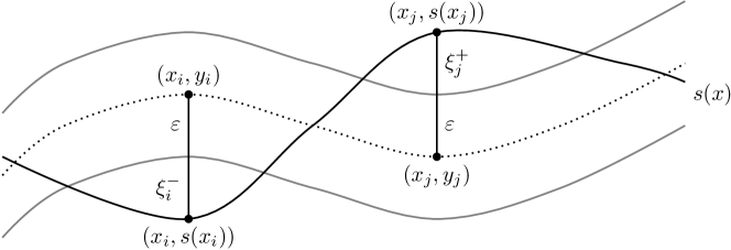
Figure 1: Illustration of the role of the slack variables in (17).

Instead of solving the primal problem of Corollary 32, it is more common to derive and solve the following dual problem. Here again we denote as $y\in\mathbb{R}^{n}$ the vector of all scalar training target values.

Proposition 34 (SVR - Dual form).

Let $\Omega$ be a nonempty set, $K$ a PD kernel on $\Omega$, $\lambda>0$ a regularization parameter. For any training set $(X_{n},Y_{n})$ there exists a solution $\left(\alpha^{+},\alpha^{-}\right)\in\mathbb{R}^{2n}$ of the problem

$$\min\limits_{\alpha^{+},\alpha^{-}\in\mathbb{R}^{n}} \frac{1}{4}\left(\alpha^{-}-\alpha^{+}\right)^{T}A\left(\alpha^{-}-\alpha^{+}\right)+\varepsilon\mathbbm{1}_{n}^{T}\left(\alpha^{+}+\alpha^{-}\right)+y^{T}\left(\alpha^{+}-\alpha^{-}\right)$$

s.t. $$\alpha^{+},\alpha^{-}\in[0,1/\lambda]^{n},$$ (18)

which is unique if $K$ is SPD. Moreover, a solution of (17) is given by

$$s(x):=\sum_{j=1}^{n}\frac{\alpha_{j}^{-}-\alpha_{j}^{+}}{2}K(x,x_{j}),\;\;x\in\Omega,$$ (19)

with $\xi_{i}^{+}:=\max(0,s(x_{i})-y_{i}-\varepsilon)$, $\xi_{i}^{-}:=\max(0,y_{i}-s(x_{i})-\varepsilon)$.

Proof.

We give a sketch of the proof, although a formal derivation requires more care, and we refer to [53, Chapter 9] for the details. The idea is to first derive the Lagrangian $\mathcal{L}:=\mathcal{L}(\alpha,\xi^{+},\xi^{-};\alpha^{+},\alpha^{-},\mu^{+},\mu^{-})$ for the primal problem (17) using non-negative Lagrange multipliers $\alpha^{+}$, $\alpha^{-}$, $\mu^{+}$, $\mu^{-}\in\mathbb{R}^{n}$ for the inequality constraints, and then derive the dual problem by imposing the Karush-Kuhn-Tucker (KKT) conditions (see e.g. Chapter 6 in [53]).

The Lagrangian is defined as

$$\mathcal{L}= \ \frac{1}{\lambda}\mathbbm{1}_{n}^{T}\left(\xi^{+}+\xi^{-}\right)+\alpha^{T}A\alpha+(\mu^{+})^{T}(-\xi^{+})+(\mu^{-})^{T}(-\xi^{-})$$ (20)

$$+\left(A\alpha-y-\varepsilon\mathbbm{1}_{n}-\xi^{+}\right)^{T}\alpha^{+}+\left(y-A\alpha-\varepsilon\mathbbm{1}_{n}-\xi^{-}\right)^{T}\alpha^{-}$$

$$= \left(\alpha+\alpha^{+}-\alpha^{-}\right)^{T}A\alpha+\left(\frac{1}{\lambda}\mathbbm{1}_{n}-\alpha^{+}-\mu^{+}\right)^{T}\xi^{+}+\left(\frac{1}{\lambda}\mathbbm{1}_{n}-\alpha^{-}-\mu^{-}\right)^{T}\xi^{-}$$

$$-\varepsilon\mathbbm{1}_{n}^{T}\left(\alpha^{+}+\alpha^{-}\right)-y^{T}\left(\alpha^{+}-\alpha^{-}\right).$$

Using the symmetry of $A$, the partial derivatives of $\mathcal{L}$ with respect to the primal variables can be computed as

$$\nabla_{\alpha}\mathcal{L}=2A\alpha+A(\alpha^{+}-\alpha^{-}),\;\;\nabla_{\xi^{+}}\mathcal{L}=\frac{1}{\lambda}\mathbbm{1}_{n}-\alpha^{+}-\mu^{+},\;\;\nabla_{\xi_{i}^{-}}\mathcal{L}=\frac{1}{\lambda}\mathbbm{1}_{n}-\alpha^{-}-\mu^{-},$$ (21)

and setting these three equalities to zero we obtain equations for $\alpha$, $\mu^{+},\mu^{-}$, where in particular $\alpha=\frac{1}{2}\left(\alpha^{-}-\alpha^{+}\right)$ (which is the unique solution if $A$ is invertible). Substituting these values in the Lagrangian we get

$$\mathcal{L} =\left(\alpha+\alpha^{+}-\alpha^{-}\right)^{T}A\alpha-\varepsilon\mathbbm{1}_{n}^{T}\left(\alpha^{+}+\alpha^{-}\right)-y^{T}\left(\alpha^{+}-\alpha^{-}\right)$$

$$=-\frac{1}{4}\left(\alpha^{-}-\alpha^{+}\right)^{T}A\left(\alpha^{-}-\alpha^{+}\right)-\varepsilon\mathbbm{1}_{n}^{T}\left(\alpha^{+}+\alpha^{-}\right)-y^{T}\left(\alpha^{+}-\alpha^{-}\right).$$

The remaining conditions in (34) stem from the requirements that the Lagrange multipliers are non-negative, and in particular $0\leq\mu_{i}^{+}=1/\lambda-\alpha^{+}_{i}$, i.e., $\alpha_{i}^{+}\leq 1/\lambda$, and similarly for $\alpha_{i}^{-}$. ∎

This dual formulation is particularly convenient to explain that the SVR surrogate has a built-in sparsity, i.e., the optimization process provides a solution where possibly many of the entries of $\alpha=\frac{1}{2}(\alpha^{-}-\alpha^{+})$ are zero. This behavior is in strong contrast with the case of interpolation of Section 4 where we needed to adopt special techniques to enforce this property. The points $x_{i}\in X_{n}$ with $\alpha_{i}\neq 0$ are called support vectors, which gives the name to the method.

In particular, as for the slack variables there is a clean geometric description of this sparsity pattern, that gives additional insights into the solution. To see this we remark that, in addition to the stationarity KKT conditions (21), an optimal solution satisfies also the complementarity KKT conditions

$$\alpha^{+}_{i}\left(s(x_{i})-y_{i}-\varepsilon-\xi_{i}^{+}\right) =0,\quad\alpha^{-}_{i}\left(y_{i}-s(x_{i})-\varepsilon-\xi_{i}^{-}\right) =0\$$ (22)

$$\xi^{+}_{i}\left(1/\lambda-\alpha_{i}^{+}\right) =0,\quad\xi^{-}_{i}\left(1/\lambda-\alpha^{-}_{i}\right) =0.$$ (23)

We then have the following:

1. Equations (22) state that $\alpha_{i}^{+}\neq 0$ only if $s(x_{i})-y_{i}-\varepsilon-\xi_{i}^{+}=0$, and similarly for $\alpha_{i}^{-}$. Since $\xi_{i}^{+}\geq 0$, this happens only when $s(x_{i})-y_{i}\geq\varepsilon$, i.e., only for points $(x_{i},s(x_{i}))$ which are outside or on the boundary of the $\varepsilon$-tube.

2. In particular, if $\alpha_{i}^{+}\neq 0$ it follows that $s(x_{i})-y_{i}\geq\varepsilon$, and thus $y_{i}-s(x_{i})-\varepsilon-\xi_{i}^{-}\neq 0$, and then necessarily $\alpha_{i}^{-}=0$. Thus, at most one of $\alpha_{i}^{+}$ and $\alpha_{i}^{-}$ can be nonzero.

3. Equations (23) imply that $\alpha_{i}^{+},\alpha_{i}^{-}=1/\lambda$ whenever $\xi_{i}^{+},\xi_{i}^{-}$ is nonzero, i.e., whenever $s(x_{i})$ is strictly outside of the $\varepsilon$-tube. The corresponding $x_{i}$ are called bounded support vector, and the value of the corresponding coefficients is indeed kept bounded by the value of the regularization parameter. Reducing $\lambda$, i.e., using less regularization, allows solutions with coefficients of larger magnitude.

In summary, we can then expect that if $s$ is a good approximation of the data, it will be also a sparse approximation.

We summarize the offline phase for SVR in Algorithm 5. We remark that in this case the extension to vector-valued functions is not as straightforward as for kernel interpolation, and it is thus common to train a separate SVR for each output component.

Algorithm 5 SVR - Offline phase

1:Input: training set $X_{n}\in\Omega^{n}$, $Y_{n}\in\mathbb{R}^{n}$, kernel $K$ (and kernel parameters), regularization parameter $\lambda\geq 0$, tube width $\varepsilon>0$.

2:Compute the kernel matrix $A\in\mathbb{R}^{n\times n}$, $A_{ij}:=K(x_{i},x_{j})$.

3:Solve the quadratic problem (34).

4:Set $I_{N}:=\{i:\alpha^{-}_{i}\neq 0\text{ or }\alpha^{+}_{i}\neq 0\}$.

5:Set $\alpha_{i}:=(\alpha_{i}^{-}-\alpha^{+}_{i})/2$ for $i\in I_{N}$.

6:Output: $\alpha\in\mathbb{R}^{N}$, $I_{N}$.

Remark 35 (General Support Vector Machines).

SVR is indeed one member of a vast collection of algorithms related to Support Vector Machines (SVMs). Standard SVMs solve classification problems, i.e., $Y_{n}\subset\{0,1\}$. The original algorithm has been introduced as a linear algorithm (or, in the present understanding, as limited to the linear kernel, i.e., the polynomial kernel with $a=0$, $p=1$), and it has later been extended via the kernel trick to its general kernel version in [4]. The SVR algorithms have instead been introduced in [53].

Moreover, the version presented here is usually called $\varepsilon$-SVR. There exists also another non equivalent version called $\nu$-SVR, which adds another term in the cost function multiplied by a factor $\nu\in[0,1]$. This has the role of giving an upper bound on the number of support vectors and on the fraction of training data which are outside of the $\varepsilon$-tube (see Chapter 9 in [53]).

We also remark that it is sometimes common to include in any SVM-based algorithm also an offset or bias term $b\in\mathbb{R}$, i.e., to obtain a surrogate $s(x)=\sum_{j=1}^{n}\alpha_{j}K(x,x_{j})+b$. This changes in an obvious way the primal problem (17), while the dual contains also the constraint $\sum_{i=1}^{n}\left(\alpha_{i}^{+}+\alpha_{i}^{-}\right)=0$. However, we stick here to this formulation and refer to [57] for a discussion of statistical and numerical benefits of not using this offset term, at least in the case of SPD kernels.

Remark 36 (Error estimation).

Also for SVR there is a detailed error theory, usually formulated in the framework of statistical learning theory (see [62]). Results are obtained by assuming that the dataset $(X_{n},Y_{n})$ is drawn from a certain unknown probability distribution, and then quantifying the approximation power of the surrogate. For a detailed treatment of this theory, we refer to [53, 55]. Moreover, recently also deterministic error bounds for translational invariant kernels have been proven in [43, 44].

5.1 Sequential Minimal Optimization

Although the optimization problem (34) can in principle be solved with any quadratic optimization method, there exists a special algorithm, called Sequential Minimal Optimization (SMO) that is designed for SVMs and that performs possibly much better.

SMO is an iterative method which improves an initial feasible guess for $\alpha^{+},\alpha^{-}\in\mathbb{R}^{n}$ until convergence, and the update is made such that the minimal possible number of entries of $\alpha$ are affected. In this way, very large problems can be efficiently solved. The original version of the algorithm has been introduced in [41] for SVM, and it has later been adapted to more general methods such as SVR, that we use here to illustrate the structure of its implementation.

The idea is to find at each iteration $\ell\in\mathbb{N}$ a minimal set of indexes $I^{\ell}\subset\{1,\dots,n\}$ and optimize only the variables with indexes in $I^{\ell}$. The procedure is then iterated until the optimum is reached. If the SVR includes an offset term, as explained in the previous section we have constraints

$$\alpha_{i}^{+},\alpha_{i}^{-}\in[0,1/\lambda],\;\;1\leq i\leq n,$$ (24)

$$\sum_{i=1}^{n}\left(\alpha_{i}^{+}+\alpha_{i}^{-}\right)=0.$$

Given a feasible solution $\left(\alpha_{i}^{+},\alpha_{i}^{-}\right)^{(\ell)}$ at iteration $\ell\in\mathbb{N}$, it is thus not possible to update a single entry of $\alpha_{i}^{+}$ or $\alpha_{i}^{-}$ without violating the KKT conditions (since at most one between $\alpha_{i}^{+}$ and $\alpha_{i}^{-}$ need to be nonzero) or violating the second constraint. It is instead possible to select two indexes $I^{\ell}:=\{i,j\}$ and in this case we have variables $\alpha_{i}^{+},\alpha_{i}^{-},\alpha_{j}^{+},\alpha_{j}^{-}$ and we can solve the restricted quadratic optimization problem under the constraints

$$\alpha_{i}^{+},\alpha_{i}^{-}\in[0,1/\lambda],i\in I^{\ell},\;\;\;\;\sum_{i\in I^{\ell}}\left(\alpha_{i}^{+}+\alpha_{i}^{-}\right)=R^{\ell}:=-\sum_{i\notin I^{\ell}}\left(\alpha_{i}^{+}+\alpha_{i}^{-}\right),$$

which can be solved analytically.

The crucial step is to select $I^{\ell}$, and this is done by finding a first index that does not satisfy the KKT conditions and a second one with some heuristic. It can be proven that, if at least one of the two violates the KKT conditions, then the objective is strictly decreased and convergence is obtained. Moreover, the vectors $\alpha^{+}=\alpha^{-}=0\in\mathbb{R}^{n}$ are always feasible and can thus be used as a first guess. In practice, the iteration is stopped when a sufficiently small value of the cost function is reached.

In the case of SVR without offset discussed in the previous section the situation is even simpler, since the second constraint in (24) is not present and it is thus possible to update a single pair $\left(\alpha_{i}^{+},\alpha_{i}^{-}\right)$ at each iteration. Nevertheless, it has been proven in [57] that using also in this case two indexes improves significantly the speed of convergence. Moreover, the same paper introduces several additional details to select the pair, to optimize the restricted cost function, and to establish termination conditions.

A general version of SMO for SVR is summarized in Algorithm 6, where we assume that the function $\eta:\{1,\dots,n\}\to\{1,\dots,n\}$ implements the selection rule of $I^{\ell}$.

Algorithm 6 SMO

1:Input: training set $X_{n}\in\Omega^{n}$, $Y_{n}\in\mathbb{R}^{n}$, kernel $K$ (and kernel parameters), regularization parameter $\lambda\geq 0$, tube width $\varepsilon>0$, selection rule $\eta$, tolerance $\tau$.

2:Set $\ell:=0$ and $\left(\alpha^{+},\alpha^{-}\right)^{(0)}:=(0,0)$.

3:while $\left(\alpha^{+},\alpha^{-}\right)^{(\ell)}$ does not satisfy KKT conditions within tolerance $\tau$. do

4:     Set $\ell=\ell+1$.

5:     Set $I^{\ell}:=\{i,j\}:=\eta\left(\{1,\dots,n\}\right)$.

6:     Set $\left(\alpha_{k}^{+},\alpha_{k}^{-}\right)^{(\ell)}:=\left(\alpha^{+}_{k},\alpha_{k}^{-}\right)^{(\ell-1)}$ for $k\notin I^{\ell}$.

7:     Solve the optimization problem restricted to $I^{\ell}$.

8:end while

9:Set $I_{N}:=\{i:\alpha^{-}_{i}\neq 0\text{ or }\alpha^{+}_{i}\neq 0\}$.

10:Set $\alpha_{i}:=(\alpha_{i}^{-}-\alpha^{+}_{i})/2$ for $i\in I_{N}$.

11:Output: $\alpha\in\mathbb{R}^{N}$, $I_{N}$.

Remark 37 (Reference implementations).

We remark that there exists commonly used implementations of SVR (and other SVM-related algorithms), which are available in several programming languages and implement also some version of this algorithm. We mention especially LIBSVM [9] and liquidSVM [58].

6 Model analysis using the surrogate

Apart from predicting new inputs with good accuracy and a significant speedup, the surrogate model can be used to perform a variety of different tasks related to meta-modeling, such as uncertainty quantification and state estimation. This can be done in a non-intrusive way, meaning that the full model is employed as a black-box that provides input-output pairs to train the surrogate, but is not required to be modified.

In principle, any kind of analysis that requires multiple evaluations can be significantly accelerated by the use of a surrogate, including the ones that are not computationally feasible due to the high computational cost of the full model. An example is uncertainty quantification, where the expected value of $f$ can be approximated by a Monte Carlo integration of $s$ using a set $X_{m}\subset\Omega$ of integration points, i.e.,

$$\int_{\Omega}f(x)dx\approx\frac{1}{m}\sum_{i=1}^{m}s(x_{i}).$$

Once the surrogate is computed using a training set $(X_{n},Y_{n})$, this approximate integral can be evaluated also for $m\gg n$ with a possibly very small cost, since the evaluation of $s$ is significantly cheaper than the one of $f$.

Another example, which we describe in detail in the following, is the solution of an inverse problem to estimate the input parameter which generated a given output, i.e., from a given vector $\overline{y}\in\mathbb{R}^{q}$ we want to estimate $x\in\Omega$ such that $f(\overline{x})=\overline{y}$. This can be done by considering a state-estimation cost function $C:\Omega\to\mathbb{R}$ defined by

$$C(x):=\frac{1}{2\left\|\overline{y}\right\|_{2}^{2}}\left\|s(x)-\overline{y}\right\|_{2}^{2},$$ (25)

and estimating $\overline{x}$ by the value $x^{*}$ defined as

$$x^{*}:=\min_{x\in\Omega}C(x).$$

In principle, we could perform the same optimization also using $f$ instead of $s$ in (25), but the surrogate allows a rapid evaluation of $C$. Moreover, if $K$ is at least differentiable, then also $s$ is differentiable, and thus we can use gradient-based methods to minimize $C$.

To detail this approach, we assume $f:\Omega\to\mathbb{R}^{q}$ and to have a surrogate obtained as in Section 4.1 with the separable matrix valued kernel of Section 2.4, i.e., from (10) we have

$$s_{N}(x)=\sum_{k\in I_{N}}\alpha_{k}K(x,x_{k}).$$

As explained in (9), in the vector-valued case $q>1$ we always assume that the output $s_{N}(x)$ and the coefficients $\alpha_{k}$ are row vectors, and in particular $\alpha\in\mathbb{R}^{N\times q}$ and $s_{N}(x)\in\mathbb{R}^{1\times q}$. In this case we have the following.

Proposition 38 (Gradient of the state estimation cost).

For $x\in\Omega\subset\mathbb{R}^{d}$ and $\overline{y}\in\mathbb{R}^{q}$, the gradient of the cost (25) can be computed in $x\in\Omega$ as

$$\nabla C(x)=\frac{1}{\left\|\overline{y}\right\|_{2}^{2}}(D\alpha)E^{T},$$

where $D\in\mathbb{R}^{d\times N}$ with columns $D_{j}:=\nabla_{x}K(x,x_{j})$, and $E:=s_{N}(x)-\overline{y}\in\mathbb{R}^{1\times q}$.

Proof.

By linearity, the gradient of $s_{N}$ in $x$ can be computed as

$$\nabla s_{N}(x)=\sum_{j=1}^{n}\alpha_{j}\nabla_{x}K(x,x_{j})=D\alpha\in\mathbb{R}^{d\times q},$$

and thus

$$\nabla C(x) =\frac{1}{\left\|\overline{y}\right\|_{2}^{2}}\left(s_{N}(x)-\overline{y}\right)\nabla_{x}\left(s_{N}(x)-\overline{y}\right)=\frac{1}{\left\|\overline{y}\right\|_{2}^{2}}\left(s_{N}(x)-\overline{y}\right)\nabla s(x)$$

$$=\frac{1}{\left\|\overline{y}\right\|_{2}^{2}}(D\alpha)E^{T}.$$

∎

Observe in particular that whenever $K$ is known in closed form the matrix $D$ can be explicitly computed, and thus the gradient can be assembled using only matrix-vector multiplications of matrices of dimensions $N,d,q$, but independent of $n$. The solution $x^{*}$ can then be computed by any gradient-based optimization method, and each iteration can be performed in an efficient way.

7 Parameter and model selection

For all the methods that we have seen the approximation quality of the surrogate depends on several parameters, which need to be carefully chosen to obtain good results. There are both parameters defining the kernel, such as the shape parameter $\gamma>0$ in a RBF kernel, and model parameters such as the regularization parameter $\lambda\geq 0$. To some extent, also the selection of the kernel itself can be considered as a parametric dependence of the model. Moreover, it is essential to test the quality of the surrogate on an independent test set of data, since tuning it on the training set alone can very likely lead to overfitting, i.e., to obtain a model that is excessively accurate on the training set, while failing to generalize its prediction capabilities to unseen data.

In practical applications the target function $f$ is unknown, so it cannot be used to check if the approximation is good, and all we know is the training set $(X_{n},Y_{n})$. In this case the most common approach is to split the sets into train, validation and test sets in the following sense. We permute $(X_{n},Y_{n})$, fix numbers $n_{tr}$, $n_{val}$, $n_{te}$ such that $n=n_{tr}+n_{val}+n_{te}$, and define a partition of the dataset as

$$X_{tr} :=\{x_{i},1\leq i\leq n_{tr}\}$$

$$X_{val} :=\{x_{i},{n_{tr}+1}\leq i\leq n_{tr}+n_{val}\}$$

$$X_{te} :=\{x_{i},{n_{tr}+n_{val}+1}\leq i\leq n\},$$

and similarly for $Y_{tr}$, $Y_{val}$, $Y_{te}$.

The idea is then to use the validation set $\left(X_{val},Y_{val}\right)$ to validate (i.e., choose) the parameters, and the test set $\left(X_{te},Y_{te}\right)$ to evaluate the error. Having disjoint sets allows to have a fair way to test the algorithm.

For the process we also need an error function that returns the error of the surrogate $s$ evaluated on a generic set of points $X:=\{x_{i}\}_{i}\subset\Omega$ w.r.t. the exact values $Y:=\{y_{i}\}_{i}$. We denote as $|X|$ the number of elements of $X$. Common examples are the maximal error and the Root Mean Square Error (RMSE) defined as

$$E\left(s,X,Y\right):=\max_{1\leq i\leq|X|}\|s(x_{i})-y_{i}\|_{2}\;\text{ or }\;E\left(s,X,Y\right):=\sqrt{\frac{1}{|X|}\sum_{i=1}^{|X|}\left\|s(x_{i})-y_{i}\right\|_{2}^{2}}.$$ (26)

Then one chooses a set of possible parameter instantiations $\{p_{1},\dots,p_{n_{p}}\}$, $n_{p}\in\mathbb{N}$ that has to be checked. A common choice for positive numerical parameters is to take them logarithmically equally spaced, since the correct scale is not known in advance, in general.

The training and validation process is described in Algorithm 7, where we denote as $s(p_{i})$ the surrogate obtained with parameter $p_{i}$. It works as an outer loop with respect to the training of any of the surrogates that we have considered, and it has thus to be understood as part of the offline phase.

Algorithm 7 Model selection by validation

1:Input: $X_{{tr}},X_{{val}},X_{{te}}$,$Y_{{tr}},Y_{{val}},Y_{{te}}$, $\{p_{1},\dots,p_{n_{p}}\}$

2:for $i=1,\dots,n_{p}$ do

3:     Train surrogate $s(p_{i})$ with data $(X_{tr},Y_{tr})$

4:     Compute validation error $e_{i}:=E(s(p_{i}),X_{val},Y_{val})$

5:end for

6:Choose parameter $\bar{p}:=p_{i}$ with $i:=\operatorname*{arg\min}e_{i}$

7:Train surrogate $s(\bar{p})$ with data $(X_{tr}\cup X_{val},Y_{tr}\cup Y_{val})$

8:Compute test error $\bar{E}=E(s(\bar{p}),X_{te},Y_{te})$

9:Output: surrogate $s(\bar{p})$, optimal parameter $\bar{p}$, test error $\bar{E}$

A more advanced way to realize the same idea is via $k$-fold cross validation. To have an even better selection of the parameters, one can repeat the validation step (lines 2-6 in the previous algorithm) by changing the validation set at each step. To do so we do not select a validation set (so $n=n_{tr}+n_{te}$), and instead consider a partition of $X_{tr},Y_{tr}$ into a fixed number $k\in\{1,\dots,n_{tr}\}$ of disjoint subsets, all approximately of the same size, i.e.,

$$X_{tr} :=\{x_{i},1\leq i\leq n_{tr}\}:=\cup_{i=1}^{k}X_{i}$$

$$X_{te} :=\{x_{i},{n_{tr}+1}\leq i\leq n\},$$

and similarly for $Y_{tr}:=\cup_{i=1}^{k}Y_{i}$ and for $Y_{te}$. In the validation step each of the the $X_{i}$ is used as a validation set, and the validation is repeated for all $i=1,\dots,k$. In this case the error $e_{i}$ for the parameter $p_{i}$ is defined as the average error over all these permutations, as described in Algorithm 8.

Algorithm 8 Model selection by $k$-fold cross validation

1:Input: $X_{tr}=\cup_{i=1}^{k}X_{i},X_{{te}}$, $Y_{tr}=\cup_{i=1}^{k}Y_{i},Y_{{te}}$, $\{p_{1},\dots,p_{n_{p}}\}$

2:for $i=1,\dots,n_{p}$ do

3:     for $j=1,\dots,k$ do

4:         Train surrogate $s(p_{i})$ with data $\left(\cup_{\ell\neq j}X_{\ell},\cup_{\ell\neq j}Y_{\ell}\right)$

5:         Compute error $e^{(j)}:=E(s(p_{i}),X_{j},Y_{j})$

6:     end for

7:     $e_{i}:=\text{mean}\{e^{(j)},1\leq j\leq k\}$

8:end for

9:Choose parameter $\bar{p}:=p_{i}$ with $i:=\operatorname*{arg\min}e_{i}$

10:Train surrogate $s(\bar{p})$ with data $(X_{tr},Y_{tr})$

11:Compute test error $\bar{E}=E(s(\bar{p}),X_{te},Y_{te})$

12:Output: surrogate $s(\bar{p})$, optimal parameter $\bar{p}$, test error $\bar{E}$

We remark that, in the extreme case $k=N$, this $k$-fold cross validation is usually called Leave One Out Cross Validation (LOOCV).

8 Numerical examples

For the testing and illustration of the two methods of Section 4 and Section 5, we consider a real-world application dataset describing the biomechanical modeling of the human spine introduced and studied in [69]. We refer to that paper for further details and we just give a brief description in the following.

The input-output function $f:\mathbb{R}^{3}\to\mathbb{R}^{3}$ represents the coupling between a global multibody system (MBS) and a Finite Elements (FEM) submodel. The human spine is represented as a MBS consisting of the vertebra, which are coupled by the interaction through intervertebral disks (IVDs). The PDE representing the behavior of each IVD is approximated by a FEM discretization, and it has the input geometry parameters as boundary conditions, and computes the output mechanical response as a result of the simulation. In particular, the three inputs are two spatial displacements and an angular inclination of a vertebra, and the three outputs are the corresponding two force components and the momentum which are transfered to the next vertebra. The dataset is generated by running the full model for $n:=1370$ different input parameters $X_{n}$ and generating the corresponding set of outputs $Y_{n}$.

The dataset, as described in Section 7, is first randomly permuted and then divided in training and test datasets $\left(X_{n_{tr}},Y_{n_{tr}}\right)$, $\left(X_{n_{te}},Y_{n_{te}}\right)$ with $n_{tr}:=1238$ and $n_{te}=132$, corresponding to roughly $90\%$ and $10\%$ of the data. We remark that the full model predicts a value $(0,0,0)^{T}$ for the input $(0,0,0)^{T}$ and this sample pair is present in the dataset. We thus manually include it in the training set independently of the permutation. The training and test sets can be seen in Figure 2.

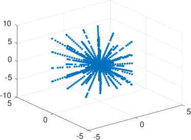
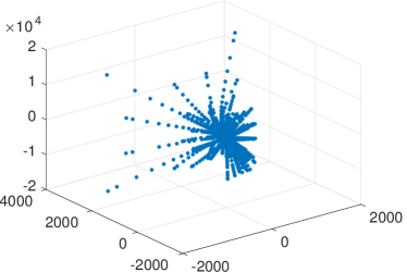
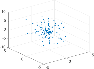
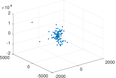
Figure 2: Input parameters (left) and corresponding outputs (right) for the training (top row) and test set (bottom row).

The models are trained using a Matlab implementation of the algorithms. For VKOGA we use an own implementation, while for SVR we employ the KerMor package, which provides an implementation of the $2$-index SMO for the SVR without offset that is discussed in Section 5.1. We remark that this implementation requires the output data to be scaled in $[-1,1]$, and thus we perform this scaling for the training and validation, while the testing is executed by scaling back the predictions to the original range. To have a fair comparison, we use the same data normalization also for the VKOGA models.

The regularized VKOGA (with $f$-, $P$-, and $f/P$-greedy selection rules) and the SVR models are trained with the Gaussian kernel. Both algorithms depend on the shape parameter $\gamma$ of the kernel and on the regularization parameter $\lambda$, while SVR additionally depends on the width $\varepsilon$ of the tube. These parameters are selected by $k$-fold cross validation as described in Section 7. The values of $k$ and of the parameter samples used for validation are reported in Table 1, where each parameter set is obtained by generating logarithmically equally spaced samples in the given interval, i.e., $400$ parameter pairs are tested for VKOGA and $4000$ triples for SVR. As an error measure we use the $\max$ error in (26). We remark that the SVR surrogate is obtained by training a separate model for each output, as described in Section 5, but only one cross validation is used. This means that for each parameter triple three models are trained, and then the parameter is evaluated in the prediction of the three dimensional output.

Moreover, the training of the VKOGA surrogates is terminated when the square of the power function is below the tolerance $\tau_{P}:=10^{-12}$, or when the training error is below the tolerance $\tau_{f}:=10^{-6}$. Additionally, it would be possible to use a maximal number of selected points as stopping criterion, and this offers the significant advantage of directly controlling the expansion size, which could be reduced to any given number (of course at the price of a reduced accuracy). In the case of SVR, instead, the number $N$ is a result of the tuning of the remaining parameters.

$k$	$\gamma_{\min}$	$\gamma_{\max}$	$n_{\gamma}$	$\lambda_{\min}$	$\lambda_{\max}$	$n_{\lambda}$	$\varepsilon_{\min}$	$\varepsilon_{\max}$	$n_{\varepsilon}$
$5$	$10^{-2}$	$10^{1}$	$20$	$10^{-16}$	$10^{3}$	$20$	$10^{-10}$	$10^{-3}$	$10$

Table 1: Parameters ranges and sample numbers used in the $k$-fold cross validation.

In Table 2 we report the values of the parameters selected by the validation procedure for the four models, as well as the number $N$ of nonzero coefficients in the trained kernel expansions. Observe that for SVR the three values of $N$ refer to the number of support vectors for the three scalar-valued models. Moreover, the number of support vectors or kernel centers is only slightly larger for SVR than for the VKOGA models, but, as discussed in the following, the VKOGA models give prediction errors which are up to two orders of magnitude smaller than the ones of the SVR model.

Method	$N$	$\bar{\gamma}$	$\bar{\lambda}$	$\bar{\varepsilon}$
VKOGA $P$-greedy	$1000$	$4.9\cdot 10^{-2}$	$10^{-11}$	–
VKOGA $f$-greedy	$879$	$4.3\cdot 10^{-2}$	$10^{-11}$	–
VKOGA $f/P$-greedy	$967$	$6.2\cdot 10^{-2}$	$10^{-9}$	–
SVR, output 1	$359$	$1.8\cdot 10^{-1}$	$10^{2}$	$7.7\cdot 10^{-7}$
output 2	$378$
output 3	$405$

Table 2: Selected parameters and number of nonzero coefficients in the kernel expansions.

We can now test the four models in the prediction on the test set. Table 3 contains various error measures between the prediction of the surrogates and the exact data. We report the values of the maximum error $E_{\max}$ and the RMSE $E_{RMSE}$ defined in (26), and the relative maximum error $E_{\max,rel}$ obtained by scaling each error by the norm of the exact output.

Method	$E_{\max}$	$E_{RMSE}$	$E_{\max,rel}$
VKOGA $P$-greedy	$1.6\cdot 10^{2}$	$22.3$	$2.2\cdot 10^{-1}$
VKOGA $f$-greedy	$1.6\cdot 10^{2}$	$22.4$	$2.0\cdot 10^{-1}$
VKOGA $f/P$-greedy	$1.6\cdot 10^{2}$	$23.2$	$8.8\cdot 10^{-1}$
SVR	$1.3\cdot 10^{3}$	$1.6\cdot 10^{2}$	$1.4\cdot 10^{1}$

Table 3: Test errors: maximum error $E_{\max}$, RMSE error $E_{RMSE}$, maximum relative error $E_{\max,rel}$

To provide a better insight in the approximation quality of the methods, we show in Figure 3 the distribution of the error over the test set. The plots show, for each sample $(x_{i},y_{i})$ in the test set, the absolute error $\left\|y_{i}-s(x_{i})\right\|_{2}$ as a function of the magnitude $\left\|y_{i}\right\|_{2}$ of the output. Moreover, the black lines represent a relative error from $10^{0}$ to $10^{-3}$. It is clear that in all cases the maximum and RMS errors of Table 3 are dominated by the values obtained for outputs of large norm, where the VKOGA models obtain a much better accuracy than SVR. The relative errors, on the other hand, are not evenly distributed for SVR, where most of the test set is approximated with a relative error between $10^{1}$ and $10^{-2}$ except for the samples with small magnitude of the output. For these data, the model gives increasingly bad predictions as the magnitude is smaller, reaching a relative error much larger than $1$. The VKOGA models, instead, obtain a relative error smaller than $10^{-2}$ on the full test set except for the entries of small magnitude. For these samples, the $f$- and $P$-greedy versions of the algorithm perform almost the same and better than the $f/P$-greedy variant, thus giving an overall smaller relative error in Table 3. Moreover, these results are obtained with a significantly smaller expansion size for $f$-greedy than for $P$-greedy. Indeed, even if the SVR surrogates for the individual output components are smaller than the VKOGA ones, the overall number of non-zero coefficients is $359+378+405=1142$, i.e., more than the one of each of the three VKOGA models, thus leading to a less accurate and more expensive surrogate.

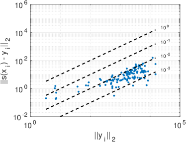
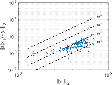
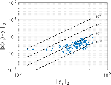
Figure 3: Absolute errors as functions of the magnitude of the output, and relative error levels from $10^{0}$ to $10^{-3}$ for the surrogates obtained with $P$-greedy VKOGA (top left), $f$-greedy VKOGA (top right), $f/P$-greedy VKOGA (bottom left) and SVR (bottom right).

Regarding the runtime requirements, we can now estimate both the offline (training) and online (prediction) times. The offline time required for the validation and training of the models is essentially determined by the number of parameters tested in the $k$-fold cross validation, while the training time of a single model is almost negligible. As a comparison, we report in Table 4 the average runtime $\tilde{T}_{offline}$ for $10$ runs of the training of the models for the fixed set of parameters of Table 2. All the reported times are in the ranges of seconds (for VKOGA) and below one minute (for SVR). We remark that this timing is only a very rough indication and not a precise comparison, since the times highly depends on the number of selected points (for VKOGA) and the number of support vectors for SVR, and both are dependent on the used parameters. For example, we repeated the experiment for SVR with the same parameter set but with $\varepsilon=10^{-1}$. In this case this value of $\varepsilon$ is overly large (if compared to the the one selected by cross validation) and it likely produces a useless model, but nevertheless we obtain an average training time of $0.03$ sec.

A more interesting comparison is the online time, which directly determines the efficiency of the surrogate models in the replacement of the full simulation. In this case, we evaluate the models $5000$ times on the full test set consisting of $n_{te}=132$ samples, and we report the average online time $\tilde{T}_{online}$ per single test sample in Table 4. The table contains also again the number $N$ of elements of the corresponding kernel expansions, and it is evident that a smaller value leads to a faster evaluation of the model.

In the original paper [69], it has been estimated that a $30$ sec full simulation with $24$ IVDs with a timestep $\Delta t=10^{-3}$ sec requires $7.2\cdot 10^{5}$ evaluations of the coupling function $f$, and these were estimated to require $600$ h. This corresponds to an average of $\tilde{T}_{full}=3$ sec per evaluation of $f$, giving a speedup $\tilde{T}_{full}/\tilde{T}_{online}$ as reported in Table 4.

Method	$N$	$\tilde{T}_{offline}$	$\tilde{T}_{online}$	$\tilde{T}_{full}/\tilde{T}_{online}$
VKOGA $P$-greedy	$1000$	$1.67$ sec	$9.97\cdot 10^{-6}$ sec	$3.01\cdot 10^{5}$
VKOGA $f$-greedy	$879$	$1.41$ sec	$9.44\cdot 10^{-6}$ sec	$3.18\cdot 10^{5}$
VKOGA $f/P$-greedy	$967$	$1.66$ sec	$9.92\cdot 10^{-6}$ sec	$3.02\cdot 10^{5}$
SVR ($3$ models)	$1142$	$52.0$ sec	$2.28\cdot 10^{-5}$ sec	$1.32\cdot 10^{5}$

Table 4: Average offline time (training only), online time, and projected speedup factor for the four different models.

These surrogates can now be employed to solve different tasks that require multiple evaluations of $f$. As an example, we employ the $f$-greedy model (as the most accurate and most efficient) to solve a parameter estimation problem as described in Section 6. We consider the output values $Y_{n_{te}}$ in the test set as a set of measures that have not been used in the training of the model, and we try to estimate the values of $X_{n_{te}}$. For each output vector $y_{i}\in\mathbb{R}^{3}$ we define a target value $\overline{y}:=y_{i}+\eta\left\|y_{i}\right\|_{2}v$ to define the cost (25), where $v\in\mathbb{R}^{3}$ is a uniform random vector representing some noise, and $\eta\in[0,1]$ is a noise level. We then use a built-in Matlab optimizer with the gradient of Proposition 38, with initial guess $x_{0}:=0\in\mathbb{R}^{3}$, to obtain an estimate $x_{i}^{*}$ of $x_{i}$. The results of the estimate for each output value in the test set are depicted in Figure 4 for $\eta=0,0.1$, where we report also the final value of the cost function $C(x_{i}^{*})$. In all cases, the optimizer seems to converge, since the value of the cost function is in all cases smaller than $10^{-4}$, which represents a relative value smaller than $10^{-3}$ with respect to the magnitude of the input values. The maximum absolute error in the estimations is quite uniform for all the samples in the test set, and this results in a good relative error of about $10^{-1}$ for large inputs, while for inputs of very small magnitude the relative error is larger than $1$, and a larger noise level leads to less accurate predictions. This behavior is coherent with the analysis of the test error discussed above, since the approximant is less accurate on inputs of small magnitude, and thus it provides a less reliable surrogate in the cost function.

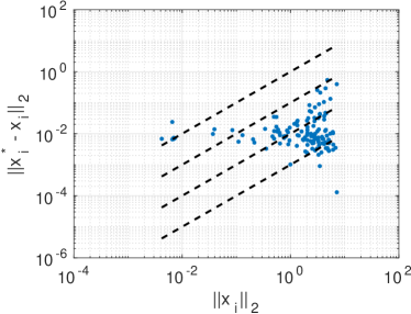
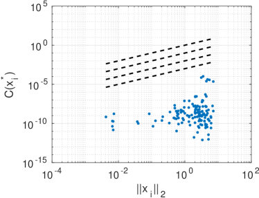
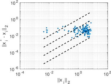
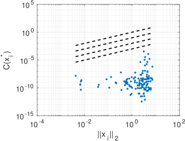
Figure 4: Absolute errors of the input estimation as functions of the magnitude of the output (left), and value of the cost function at the estimated input (right) for a noise level $\eta=0$ (top row) and $\eta=0.1$ (bottom row) using the $f$-greedy VKOGA model. The dotted lines represent relative error levels from $10^{0}$ to $10^{-3}$.

9 Summary and perspectives

In this chapter we discussed the use of kernel methods to construct surrogate models based on scattered data samples. These methods can be applied to data with general structure, and they scale well with the dimension of the input and output values. In particular, we analyzed issues and methods to obtain sparse solutions, which are then extremely fast to evaluate, while still being very accurate. These properties have been further demonstrated on numerical tests on a real application dataset. These methods can be analyzed in the common framework of Reproducing Kernel Hilbert Spaces, which provides solid theoretical foundations and a high flexibility to derive new algorithms.

The integration of machine learning and model reduction is promising and many interesting aspects have still to be investigated. For example, surrogate models have been used in [23, 24] to learn a representation with respect to projection-based methods, and generally a more extensive application of machine learning to dynamical systems requires additional understanding and the derivation of new techniques. Moreover, the field of data-based numerics is very promising, where classical numerical methods are integrated or accelerated with data-based models.

References

- [1] M. Alvarez, L. Rosasco, and N. D. Lawrence. Kernels for vector-valued functions: a review. Foundations and Trends in Machine Learning, 4(3):195–266, 2012.
- [2] N. Aronszajn. Theory of reproducing kernels. Transactions of the American Mathematical Society, 68:337–404, 1950.
- [3] A. Beckert and H. Wendland. Multivariate interpolation for fluid-structure-interaction problems using radial basis functions. Aerospace Science and Technology, 5(2):125–134, 2001.
- [4] B. E. Boser, I. M. Guyon, and V. N. Vapnik. A training algorithm for optimal margin classifiers. In Proceedings of the Fifth Annual Workshop on Computational Learning Theory, COLT ’92, pages 144–152, New York, NY, USA, 1992. ACM.
- [5] J. Bouvrie and B. Hamzi. Kernel methods for the approximation of nonlinear systems. SIAM Journal on Control and Optimization, 55(4):2460–2492, 2017.
- [6] T. Brünnette, G. Santin, and B. Haasdonk. Greedy kernel methods for accelerating implicit integrators for parametric ODEs. In F. A. Radu, K. Kumar, I. Berre, J. M. Nordbotten, and I. S. Pop, editors, Numerical Mathematics and Advanced Applications - ENUMATH 2017, pages 889–896, Cham, 2019. Springer International Publishing.
- [7] R. Cavoretto, A. De Rossi, and E. Perracchione. Efficient computation of partition of unity interpolants through a block-based searching technique. Comput. Math. Appl., 71(12):2568–2584, June 2016.
- [8] R. Cavoretto, G. Fasshauer, and M. McCourt. An introduction to the Hilbert-Schmidt SVD using iterated Brownian bridge kernels. Numerical Algorithms, 68(2):1–30, Feb 2014.
- [9] C.-C. Chang and C.-J. Lin. LIBSVM: A library for support vector machines. ACM Transactions on Intelligent Systems and Technology, 2:27:1–27:27, 2011. Software available at http://www.csie.ntu.edu.tw/~cjlin/libsvm.
- [10] S. Chen, D. Donoho, and M. Saunders. Atomic decomposition by basis pursuit. SIAM Journal on Scientific Computing, 20(1):33–61, 1998.
- [11] W. Chen, Z.-J. Fu, and C.-S. Chen. Recent advances in radial basis function collocation methods. Springer, 2014.
- [12] S. Deparis, D. Forti, and A. Quarteroni. A rescaled localized Radial Basis Function interpolation on non-Cartesian and nonconforming grids. SIAM Journal on Scientific Computing, 36(6):A2745–A2762, 2014.
- [13] S. Deparis, D. Forti, and A. Quarteroni. A Fluid–Structure Interaction Algorithm Using Radial Basis Function Interpolation Between Non-Conforming Interfaces, pages 439–450. Springer International Publishing, Cham, 2016.
- [14] M. Drohmann and K. Carlberg. The ROMES method for statistical modeling of Reduced-Order-Model error. SIAM/ASA Journal on Uncertainty Quantification, 3(1):116–145, 2015.
- [15] G. E. Fasshauer and M. McCourt. Kernel-Based Approximation Methods Using MATLAB, volume 19 of Interdisciplinary Mathematical Sciences. World Scientific Publishing Co. Pte. Ltd., Hackensack, NJ, 2015.
- [16] G. E. Fasshauer and M. J. McCourt. Stable evaluation of Gaussian radial basis function interpolants. SIAM J. Sci. Comput., 34(2):A737–A762, 2012.
- [17] B. Fornberg and N. Flyer. A primer on radial basis functions with applications to the geosciences. SIAM, 2015.
- [18] B. Fornberg, E. Larsson, and N. Flyer. Stable computations with Gaussian radial basis functions. SIAM J. Sci. Comput., 33(2):869–892, 2011.
- [19] J. Garcke and M. Griebel. Sparse grids and applications, volume 88. Springer Science & Business Media, 2012.
- [20] T. Gärtner, J. W. Lloyd, and P. A. Flach. Kernels for structured data. In S. Matwin and C. Sammut, editors, Inductive Logic Programming, pages 66–83, Berlin, Heidelberg, 2003. Springer Berlin Heidelberg.
- [21] I. Goodfellow, Y. Bengio, and A. Courville. Deep Learning. MIT Press, 2016. http://www.deeplearningbook.org.
- [22] S. Grundel, N. Hornung, B. Klaassen, P. Benner, and T. Clees. Computing Surrogates for Gas Network Simulation Using Model Order Reduction, pages 189–212. Springer New York, New York, NY, 2013.
- [23] M. Guo and J. S. Hesthaven. Reduced order modeling for nonlinear structural analysis using Gaussian process regression. Computer Methods in Applied Mechanics and Engineering, 341:807–826, 2018.
- [24] M. Guo and J. S. Hesthaven. Data-driven reduced order modeling for time-dependent problems. Computer Methods in Applied Mechanics and Engineering, 345:75–99, 2019.
- [25] B. Haasdonk and G. Santin. Greedy kernel approximation for sparse surrogate modeling. In W. Keiper, A. Milde, and S. Volkwein, editors, Reduced-Order Modeling (ROM) for Simulation and Optimization: Powerful Algorithms as Key Enablers for Scientific Computing, pages 21–45. Springer International Publishing, Cham, 2018.
- [26] D. Haussler. Convolution kernels on discrete structures, 1999.
- [27] G. S. Kimeldorf and G. Wahba. A correspondence between Bayesian estimation on stochastic processes and smoothing by splines. Ann. Math. Statist., 41(2):495–502, 04 1970.
- [28] M. Köppel, F. Franzelin, I. Kröker, S. Oladyshkin, G. Santin, D. Wittwar, A. Barth, B. Haasdonk, W. Nowak, D. Pflüger, and C. Rohde. Comparison of data-driven uncertainty quantification methods for a carbon dioxide storage benchmark scenario. Computational Geosciences, 23(2):339–354, Apr 2019.
- [29] T. Köppl, G. Santin, B. Haasdonk, and R. Helmig. Numerical modelling of a peripheral arterial stenosis using dimensionally reduced models and kernel methods. International Journal for Numerical Methods in Biomedical Engineering, 34(8):e3095, 2018. e3095 cnm.3095.
- [30] M. Kowalewski, E. Larsson, and A. Heryudono. An adaptive interpolation scheme for molecular potential energy surfaces. The Journal of Chemical Physics, 145(8):084104, 2016.
- [31] E. Larsson, E. Lehto, A. Heryudono, and B. Fornberg. Stable computation of differentiation matrices and scattered node stencils based on Gaussian radial basis functions. SIAM Journal on Scientific Computing, 35(4):A2096–A2119, 2013.
- [32] A. Manzoni and F. Negri. Heuristic strategies for the approximation of stability factors in quadratically nonlinear parametrized PDEs. Advances in Computational Mathematics, 41(5):1255–1288, 2015.
- [33] E. Marchandise, C. Piret, and J.-F. Remacle. CAD and mesh repair with Radial Basis Functions. Journal of Computational Physics, 231(5):2376–2387, 2012.
- [34] I. Martini. Reduced Basis Approximation for Heterogeneous Domain Decomposition Problems. PhD thesis, IANS, University of Stuttgart, 2017.
- [35] C. A. Micchelli and M. Pontil. On learning vector-valued functions. Neural Comput., 17(1):177–204, 2005.
- [36] S. Müller. Komplexität und Stabilität von kernbasierten Rekonstruktionsmethoden (Complexity and Stability of Kernel-based Reconstructions). PhD thesis, Fakultät für Mathematik und Informatik, Georg-August-Universität Göttingen, 2009.
- [37] S. Müller and R. Schaback. A Newton basis for kernel spaces. J. Approx. Theory, 161(2):645–655, 2009.
- [38] R. A. Olea. Geostatistics for engineers and earth scientists. Springer Science & Business Media, 2012.
- [39] M. Pazouki and R. Schaback. Bases for kernel-based spaces. J. Comput. Appl. Math., 236(4):575–588, 2011.
- [40] B. Peherstorfer and Y. Marzouk. A transport-based multifidelity preconditioner for Markov chain Monte Carlo. ArXiv 1808.09379, 2018.
- [41] J. Platt. Sequential minimal optimization: A fast algorithm for training support vector machines. Technical report, April 1998.
- [42] C. E. Rasmussen and C. K. I. Williams. Gaussian Processes for Machine Learning. The MIT Press, 2006.
- [43] C. Rieger and B. Zwicknagl. Sampling inequalities for infinitely smooth functions, with applications to interpolation and machine learning. Adv. Comput. Math., 32(1):103, 2008.
- [44] C. Rieger and B. Zwicknagl. Deterministic error analysis of support vector regression and related regularized kernel methods. J. Mach. Learn. Res., 10:2115–2132, Dec. 2009.
- [45] S. Saitoh and Y. Sawano. Theory of Reproducing Kernels and Applications. Developments in Mathematics; 44. Springer, Singapore, 2016.
- [46] G. Santin and B. Haasdonk. Convergence rate of the data-independent P-greedy algorithm in kernel-based approximation. Dolomites Res. Notes Approx., 10:68–78, 2017.
- [47] G. Santin, D. Wittwar, and B. Haasdonk. Greedy regularized kernel interpolation. ArXiv preprint 1807.09575, University of Stuttgart, 2018.
- [48] R. Schaback. Error estimates and condition numbers for radial basis function interpolation. Adv. Comput. Math., 3(3):251–264, 1995.
- [49] R. Schaback and H. Wendland. Approximation by positive definite kernels. In M. Buhmann and D. Mache, editors, Advanced Problems in Constructive Approximation, volume 142 of International Series in Numerical Mathematics, pages 203–221, 2002.
- [50] M. Scheuerer, R. Schaback, and M. Schlather. Interpolation of spatial data – a stochastic or a deterministic problem? European Journal of Applied Mathematics, 24(4):601–629, 2013.
- [51] A. Schmidt and B. Haasdonk. Data-driven surrogates of value functions and applications to feedback control for dynamical systems. IFAC-PapersOnLine, 51(2):307–312, 2018. 9th Vienna International Conference on Mathematical Modelling.
- [52] B. Schölkopf, R. Herbrich, and A. J. Smola. A generalized representer theorem. In D. Helmbold and B. Williamson, editors, Computational Learning Theory, pages 416–426, Berlin, Heidelberg, 2001. Springer Berlin Heidelberg.
- [53] B. Schölkopf and A. Smola. Learning with Kernels. The MIT Press, 2002.
- [54] J. Shawe-Taylor and N. Cristianini. Kernel Methods for Pattern Analysis. Cambridge University Press, 2004.
- [55] I. Steinwart and A. Christmann. Support Vector Machines. Science + Business Media. Springer, 2008.
- [56] I. Steinwart, D. Hush, and C. Scovel. An explicit description of the Reproducing Kernel Hilbert Spaces of Gaussian RBF kernels. IEEE Transactions on Information Theory, 52(10):4635–4643, Oct 2006.
- [57] I. Steinwart, D. Hush, and C. Scovel. Training SVMs Without Offset. J. Mach. Learn. Res., 12:141–202, February 2011.
- [58] I. Steinwart and P. Thomann. liquidSVM: A fast and versatile SVM package. ArXiv 1702.06899, 2017.
- [59] J. Suykens, J. Vanderwalle, and B. D. Moor. Optimal control by least squares support vector machines. Neural Networks, 14:23–35, 2001.
- [60] T. Taddei, J. D. Penn, M. Yano, and A. T. Patera. Simulation-based classification; a model-order-reduction approach for structural health monitoring. Archives of Computational Methods in Engineering, pages 1–23, 2016.
- [61] R. Tibshirani. Regression shrinkage and selection via the LASSO. Journal of the Royal Statistical Society. Series B (Methodological), 58(1):267–288, 1996.
- [62] V. Vapnik. Statistical Learning Theory. John Wiley & Sons, New York, 1998.
- [63] H. Wendland. Piecewise polynomial, positive definite and compactly supported radial functions of minimal degree. Adv. Comput. Math., 4(1):389–396, 1995.
- [64] H. Wendland. Fast evaluation of radial basis functions: methods based on partition of unity. In Approximation theory, X (St. Louis, MO, 2001), Innov. Appl. Math., pages 473–483. Vanderbilt Univ. Press, Nashville, TN, 2002.
- [65] H. Wendland. Scattered Data Approximation, volume 17 of Cambridge Monographs on Applied and Computational Mathematics. Cambridge University Press, Cambridge, 2005.
- [66] H. Wendland and C. Rieger. Approximate interpolation with applications to selecting smoothing parameters. Numerische Mathematik, 101(4):729–748, 2005.
- [67] D. Wirtz and B. Haasdonk. A-posteriori error estimation for parameterized kernel-based systems. In Proc. MATHMOD 2012 - 7th Vienna International Conference on Mathematical Modelling, 2012.
- [68] D. Wirtz and B. Haasdonk. A vectorial kernel orthogonal greedy algorithm. Dolomites Res. Notes Approx., 6:83–100, 2013.
- [69] D. Wirtz, N. Karajan, and B. Haasdonk. Surrogate modelling of multiscale models using kernel methods. International Journal of Numerical Methods in Engineering, 101(1):1–28, 2015.
- [70] D. Wittwar, G. Santin, and B. Haasdonk. Interpolation with uncoupled separable matrix-valued kernels. Dolomites Res. Notes Approx., 11:23–29, 2018.
- [71] H. Zhang, C. and L. Zhao, C.-J. On the inclusion relation of reproducing kernel Hilbert spaces. Analysis and Applications, 11, 2013.