Exploiting variable precision in GMRES

Abstract

We describe how variable precision floating-point arithmetic can be used to compute inner products in the iterative solver GMRES. We show how the precision of the inner products carried out in the algorithm can be reduced as the iterations proceed, without affecting the convergence rate or final accuracy achieved by the iterates. Our analysis explicitly takes into account the resulting loss of orthogonality in the Arnoldi vectors. We also show how inexact matrix-vector products can be incorporated into this setting.

Keywords— variable precision arithmetic, inexact inner products, inexact matrix-vector products, Arnoldi algorithm, GMRES algorithm

AMS Subject Codes— 15A06, 65F10, 65F25, 97N20

1 Introduction

As highlighted in a recent SIAM News article [17], there is growing interest in the use of variable precision floating-point arithmetic in numerical algorithms. (Other recent references include [4, 14, 15, 16, 18, 19] to cite only a few.) In this paper, we describe how variable precision arithmetic can be exploited in the iterative solver GMRES [27]. We show that the precision of some floating-point operations carried out in the algorithm can be reduced as the iterations proceed, without affecting the convergence rate or final accuracy achieved by the iterates.

There is already a literature on the use of inexact matrix-vector products in GMRES and other Krylov subspace methods; see, e.g., [28, 7, 3, 11, 29, 12] and the references therein. This work is not a simple extension of such results. To illustrate, suppose that all arithmetic operations are performed exactly, except the matrix-vector products. Then one obtains an inexact Arnoldi relation

$$AV_{k}+E_{k}=V_{k+1}H_{k},\qquad V_{k}^{T}V_{k}=I.$$ (1)

On the other hand, if only inner products are performed inexactly, the Arnoldi relation continues to hold but the orthogonality of the Arnoldi vectors is lost:

$$AV_{k}=V_{k+1}H_{k},\qquad V_{k}^{T}V_{k}=I-F_{k}.$$ (2)

Thus, to understand the convergence behaviour and maximum attainable accuracy of GMRES implemented with inexact inner products, it is absolutely necessary to understand the resulting loss of orthogonality in the Arnoldi vectors. We adapt techniques used in the rounding-error analysis of the Modified Gram-Schmidt (MGS) algorithm (see [1, 2] or [20] for a more recent survey) and of the MGS-GMRES algorithm (see [6, 13, 22]).

We focus on inexact inner products and matrix-vector products (as opposed to the other saxpy operations involved in the algorithm) because these are the two most time-consuming operations in parallel computations. The rest of the paper is organized as follows. We start with a brief discussion of GMRES in non-standard inner products in Section 2. Next, in Section 3, we analyze GMRES with inexact inner products. We then show how inexact matrix-vector products can be incorporated into this setting in Section 4. Some numerical examples are presented in Sections 5 and 6.

2 GMRES in weighted inner products

Shown below is the Arnoldi algorithm, with $\langle y,z\rangle=y^{T}z$ denoting the standard Euclidean inner product.

Algorithm 1 Arnoldi algorithm

0:  $A\in\mathbb{R}^{n\times n}$, $b\in\mathbb{R}^{n}$

1:  $\beta=\sqrt{\langle b,b\rangle}$

2:  $v_{1}=b/\beta$

3:  for $j=1,2,\dots$ do

4:     $w_{j}=Av_{j}$

5:     for $i=1,\dots,j$ do

6:        $h_{ij}=\langle v_{i},w_{j}\rangle$

7:        $w_{j}=w_{j}-h_{ij}v_{i}$

8:     end for

9:     $h_{j+1,j}=\sqrt{\langle w_{j},w_{j}\rangle}$

10:     $v_{j+1}=w_{j}/h_{j+1,j}$

11:  end for

After $k$ steps of the algorithm are performed in exact arithmetic, the output is $V_{k+1}=[v_{1},\dots,v_{k+1}]\in\mathbb{R}^{n\times(k+1)}$ and upper-Hessenberg $H_{k}\in\mathbb{R}^{(k+1)\times k}$ such that

$$v_{1}=\frac{b}{\beta},\qquad AV_{k}=V_{k+1}H_{k},\qquad V_{k}^{T}V_{k}=I_{k}.$$

The columns of $V_{k}$ form an orthonormal basis for the Krylov subspace

$${\cal K}_{k}(A,b)=\mathrm{span}\big{\{}\,b,Ab,A^{2}b,\dots,A^{k-1}b\,\big{\}}.$$

In GMRES, we restrict $x_{k}$ to this subspace: $x_{k}=V_{k}y_{k}$, where $y_{k}\in\mathbb{R}^{k}$ is the solution of

$$\min_{y}\|b-AV_{k}y\|_{2}=\min_{y}\|V_{k+1}(\beta e_{1}-H_{k}y)\|_{2}=\min_{y}\|\beta e_{1}-H_{k}y\|_{2}.$$

It follows that

$$\begin{split}&x_{k}=V_{k}y_{k}=V_{k}(H_{k}^{T}H_{k})^{-1}H_{k}^{T}(\beta e_{1})=V_{k}H_{k}^{\dagger}(\beta e_{1}),\\ &r_{k}=b-Ax_{k}=V_{k+1}(\beta e_{1}-H_{k}y_{k})=V_{k+1}(I-H_{k}H_{k}^{\dagger})\beta e_{1}.\end{split}$$ (3)

Any given symmetric positive definite matrix $W$ defines a weighted inner product $\langle y,z\rangle_{W}=y^{T}Wz$ and associated norm $\|z\|_{W}=\sqrt{\langle z,z\rangle_{W}}$. Suppose we use this inner product instead of the standard Euclidean inner product in the Arnoldi algorithm. We use tildes to denote the resulting quantities in the algorithm. After $k$ steps, the result is $\widetilde{V}_{k+1}=[\widetilde{v}_{1},\dots,\widetilde{v}_{k+1}]$ and upper-Hessenberg $\widetilde{H}_{k}\in\mathbb{R}^{(k+1)\times k}$ such that

$$\widetilde{v}_{1}=\frac{b}{\|b\|_{W}}=\frac{b}{\widetilde{\beta}},\qquad A\widetilde{V}_{k}=\widetilde{V}_{k+1}\widetilde{H}_{k},\qquad\widetilde{V}_{k}^{T}W\widetilde{V}_{k}=I_{k}.$$

The columns of $\widetilde{V}_{k}$ form a $W$-orthonormal basis for ${\cal K}_{k}(A,b)$. Let $\widetilde{x}_{k}=\widetilde{V}_{k}\widetilde{y}_{k}$, where $\widetilde{y}_{k}\in\mathbb{R}^{k}$ is the solution of

$$\min_{y}\|b-A\widetilde{V}_{k}y\|_{W}=\min_{y}\|\widetilde{V}_{k+1}(\widetilde{\beta}e_{1}-\widetilde{H}_{k}y)\|_{W}=\min_{y}\|\widetilde{\beta}e_{1}-\widetilde{H}_{k}y\|_{2},$$

so that

$$\widetilde{x}_{k}=\widetilde{V}_{k}\widetilde{H}_{k}^{\dagger}(\widetilde{\beta}e_{1}),\qquad\widetilde{r}_{k}=b-A\widetilde{x}_{k}=\widetilde{V}_{k+1}(I-\widetilde{H}_{k}\widetilde{H}_{k}^{\dagger})\widetilde{\beta}e_{1}.$$

We denote the above algorithm $W$-GMRES.

Let $x_{k}$ and $\widetilde{x}_{k}$ denote the iterates computed by standard GMRES and $W$-GMRES, respectively, with corresponding residual vectors $r_{k}$ and $\widetilde{r}_{k}$. It is well known that

$$1\leq\frac{\|\widetilde{r}_{k}\|_{2}}{\|r_{k}\|_{2}}\leq\sqrt{\kappa_{2}(W)}.$$ (4)

See e.g. [26] for a proof. Thus, if $\kappa_{2}(W)$ is small, the Euclidean norm of the residual vector in $W$-GMRES converges at essentially the same rate as in standard GMRES. A similar result [8, Theorem 4] holds for the residual computed in the quasi-minimal residual method [10, 9].

3 GMRES with inexact inner products

3.1 Preliminary results

Suppose the inner products in the Arnoldi algorithm are computed inexactly, i.e., line 6 in Algorithm 1 is replaced by

$$h_{ij}=v_{i}^{T}w_{j}+\eta_{ij},$$ (5)

with $|\eta_{ij}|$ bounded by some tolerance. Our main contribution is to show precisely how large each $\eta_{ij}$ can be without affecting the convergence of GMRES. Throughout we assume that all arithmetic operations in GMRES are performed exactly, except for the above inner products.

It is straightforward to show that despite the inexact inner products in (5), the relation $AV_{k}=V_{k+1}H_{k}$ continues to hold. On the other hand, the orthogonality of the Arnoldi vectors is lost. We have

$$[b,AV_{k}]=V_{k+1}[\beta e_{1},H_{k}],\qquad V_{k+1}^{T}V_{k+1}=I_{k+1}+F_{k}.$$ (6)

The relation between each $\eta_{ij}$ and the overall loss of orthogonality $F_{k}$ is very difficult to understand. To simplify the analysis we suppose that each $v_{j}$ is normalized exactly. (This is not an uncommon assumption; see, e.g., [1] and [21].) Under this simplification, we have

$$F_{k}=\bar{U}_{k}+\bar{U}_{k}^{T},\quad\bar{U}_{k}=\begin{bmatrix}0_{k\times 1}&U_{k}\\ 0_{1\times 1}&0_{1\times k}\end{bmatrix},\quad U_{k}=\begin{bmatrix}v_{1}^{T}v_{2}&\dots&v_{1}^{T}v_{k+1}\\ &\ddots&\vdots\\ &&v_{k}^{T}v_{k+1}\end{bmatrix},$$ (7)

i.e., $U_{k}\in\mathbb{R}^{k\times k}$ contains the strictly upper-triangular part of $F_{k}$. Define

$$N_{k}=\begin{bmatrix}\eta_{11}&\dots&\eta_{1k}\\ &\ddots&\vdots\\ &&\eta_{kk}\end{bmatrix},\quad R_{k}=\begin{bmatrix}\,h_{21}&\dots&h_{2k}\\ &\ddots&\vdots\\ &&h_{k+1,k}\end{bmatrix}.$$ (8)

Note that $R_{k}$ must be invertible if $h_{j+1,j}\neq 0$ for $j=1,\dots,k$, in other words, if GMRES has not terminated by step $k$. (We assume that GMRES does not breakdown by step $k$.) Following Björck’s seminal rounding error analysis of MGS [1], it can be shown that

$$N_{k}=-[0,U_{k}]H_{k}=-U_{k}R_{k}.$$ (9)

For completeness, a proof of (9) is provided in the appendix.

Additionally, in order to understand how $\|F_{k}\|_{2}$ increases as the residual norm decreases, we will need the following rather technical lemma. The relationship (10) is well know (see for example [28, Lemma 5.1]) while (12) is essentially a special case of [23, Theorem 4.1]. We defer the proof to the appendix.

Lemma 1.

Let $y_{j}$ and $t_{j}$ be the least squares solution and residual vector of

$$\min_{y}\|\beta e_{1}-H_{j}y\|_{2},$$

for $j=1,\dots,k$. Then

$$|e_{j}^{T}y_{k}|\leq\frac{\|t_{j-1}\|_{2}}{\sigma_{\min}(H_{k})}.$$ (10)

In addition, given $\epsilon>0$, let $D_{k}$ be any nonsingular matrix such that

$$\|D_{k}\|_{2}\leq\frac{\sigma_{\min}(H_{k})\epsilon\|b\|_{2}}{\sqrt{2}\|t_{k}\|_{2}}.$$ (11)

Then

$$\frac{\|t_{k}\|_{2}}{\big{(}\epsilon^{2}\|b\|_{2}^{2}+2\|D_{k}y_{k}\|_{2}^{2}\big{)}^{1/2}}\leq\sigma_{\min}\left(\begin{bmatrix}\epsilon^{-1}e_{1},H_{k}D_{k}^{-1}\end{bmatrix}\right)\leq\frac{\|t_{k}\|_{2}}{\epsilon\|b\|_{2}}.$$ (12)

Finally, although the columns of $V_{k+1}$ in (6) are not orthonormal in the standard Euclidean inner product, we will use the fact that there exists an inner product in which they are orthonormal. The proof of the following lemma is given in the appendix.

Lemma 2.

Consider a given matrix $Q\in\mathbb{R}^{n\times k}$ of rank $k$ such that

$$\qquad Q^{T}Q=I_{k}-F.$$ (13)

If $\|F\|_{2}\leq\delta$ for some $\delta\in(0,1)$, then there exists a matrix $M$ such that $I_{n}+M$ is symmetric positive definite and

$$Q^{T}(I_{n}+M)Q=I_{k}.$$ (14)

In other words, the columns of $Q$ are exactly orthonormal in an inner product defined by $I_{n}+M$. Furthermore,

$$\kappa_{2}(I_{n}+M)\leq\frac{1+\delta}{1-\delta}.$$ (15)

Note that $\kappa_{2}(I_{n}+M)$ remains small even for values of $\delta$ close to $1$. For example, suppose $\|I_{k}-Q^{T}Q\|_{2}=\delta=\nicefrac{{1}}{{2}}$, indicating an extremely severe loss of orthogonality. Then $\kappa_{2}(I_{n}+M)\leq 3$, so $Q$ still has exactly orthonormal columns in an inner product defined by a very well-conditioned matrix.

Remark 1.

Paige and his coauthors [2, 21, 25] have developed an alternative measure of loss of orthogonality. Given $Q\in\mathbb{R}^{n\times k}$ with normalized columns, the measure is $\|S\|_{2}$, where $S=(I+U)^{-1}U$ and $U$ is the strictly upper-triangular part of $Q^{T}Q$. Additionally, orthogonality can be recovered by augmentation: the matrix $P=\left[\begin{smallmatrix}S\\ Q(I-S)\end{smallmatrix}\right]$ has orthonormal columns. This measure was used in the groundbreaking rounding error analysis of the MGS-GMRES algorithm [22]. In the present paper, under the condition $\|F\|_{2}\leq\delta<1$, we use the measure $\|F\|_{2}$ and recover orthogonality in the $(I+M)$ inner product. However, Paige’s approach is likely to be the most appropriate for analyzing the Lanczos and conjugate gradient algorithms, in which orthogonality is quickly lost and $\|F\|_{2}>1$ long before convergence.

3.2 A strategy for bounding the $\eta_{ij}$

We now show how to bound the error $\eta_{ij}$ in (5) to ensure that the convergence of the GMRES is not affected by the inexact inner products.

The following theorem shows how the convergence of GMRES with inexact inner products relates to that of exact GMRES. The idea is similar to [22, Section 5], in which the quantity $\|E_{k}R_{k}^{-1}\|_{F}$ must be bounded, where $R_{k}$ is the matrix in (8) and $E_{k}$ is a matrix containing rounding errors.

Theorem 1.

Let $x_{k}^{\mathrm{(e)}}$ denote the $k$-th iterate of standard GMRES, performed exactly, with residual vector $r_{k}^{\mathrm{(e)}}$. Now suppose that the Arnoldi algorithm is run with inexact inner products as in (5), so that (6)–(9) hold, and let $x_{k}$ and $r_{k}$ denote the resulting GMRES iterate and residual vector. Let $y_{k}$ and $t_{k}$ be the least squares solution and residual vector of

$$\min_{y}\|\beta e_{1}-H_{k}y\|_{2}.$$

If for all steps $j=1,\dots,k$ of GMRES all inner products are performed inexactly as in (5) with tolerances bounded by

$$|\eta_{ij}|\leq\eta_{j}\equiv\frac{\phi_{j}\epsilon\sigma_{\min}(H_{k})}{\sqrt{2}}\frac{\|b\|_{2}}{\|t_{j-1}\|_{2}}$$ (16)

for any $\epsilon\in(0,1)$ and any positive numbers $\phi_{j}$ such that $\sum_{j=1}^{k}\phi_{j}^{2}\leq 1$, then at step $k$ either

$$1\leq\frac{\|r_{k}\|_{2}}{\|r_{k}^{\mathrm{(e)}}\|_{2}}\leq\sqrt{3},$$ (17)

or

$$\frac{\|t_{k}\|_{2}}{\|b\|_{2}}\leq 6k\epsilon,$$ (18)

implying that GMRES has converged to a relative residual of $6k\epsilon$.

Proof.

If (16) holds, then in (8)

$$|N_{k}|\leq\begin{bmatrix}\eta_{1}&\eta_{2}&\dots&\eta_{k}\\ &\eta_{2}&\dots&\eta_{k}\\ &&\ddots&\vdots\\ &&&\eta_{k}\end{bmatrix}=E_{k}D_{k},$$

where $E_{k}$ is an upper-triangular matrix containing only ones in its upper-triangular part, so that $\|E_{k}\|_{2}\leq k$, and $D_{k}=\mbox{diag}(\eta_{1},\dots,\eta_{k})$. Then,

$$\begin{split}\|N_{k}R_{k}^{-1}\|_{2}&\leq\|N_{k}D_{k}^{-1}\|_{2}\|D_{k}R_{k}^{-1}\|_{2}\\ &\leq\|E_{k}\|_{2}\|D_{k}R_{k}^{-1}\|_{2}\leq k\|(R_{k}D_{k}^{-1})^{-1}\|_{2}.\end{split}$$ (19)

Let $h_{k}^{T}$ denote the first row of $H_{k}$, so that $H_{k}=\left[\begin{smallmatrix}h_{k}^{T}\\ R_{k}\end{smallmatrix}\right]$. For any $\epsilon>0$ we have

$$\sigma_{\min}(R_{k}D_{k}^{-1}) =\,\min_{\|u\|_{2}=\|v\|_{2}=1}u^{T}R_{k}D_{k}^{-1}v$$

$$=\,\min_{\|u\|_{2}=\|v\|_{2}=1}\ [0,u^{T}]\begin{bmatrix}\epsilon^{-1}&h_{k}^{T}D_{k}^{-1}\\ 0&R_{k}D_{k}^{-1}\end{bmatrix}\begin{bmatrix}0\\ v\end{bmatrix}$$

$$\geq\,\min_{\|u\|_{2}=\|v\|_{2}=1}\ u^{T}\begin{bmatrix}\epsilon^{-1}&h_{k}^{T}D_{k}^{-1}\\ 0&R_{k}D_{k}^{-1}\end{bmatrix}v$$

$$=\,\sigma_{\min}\left(\begin{bmatrix}\epsilon^{-1}e_{1},H_{k}D_{k}^{-1}\end{bmatrix}\right).$$

Therefore,

$$\|(R_{k}D_{k}^{-1})^{-1}\|_{2}=\frac{1}{\sigma_{\min}(R_{k}D_{k}^{-1})}\\ \leq\frac{1}{\sigma_{\min}\left(\begin{bmatrix}\epsilon^{-1}e_{1},H_{k}D_{k}^{-1}\end{bmatrix}\right)}.$$

Notice that if the $\eta_{j}$ are chosen as in (16), $D_{k}$ automatically satisfies (11). Using the lower bound in (12), then (10) and (16), we obtain

$$\|(R_{k}D_{k}^{-1})^{-1}\|_{2} \leq\frac{\big{(}\epsilon^{2}\|b\|_{2}^{2}+2\|D_{k}y_{k}\|_{2}^{2}\big{)}^{1/2}}{\|t_{k}\|_{2}}$$

$$=\frac{\big{(}\epsilon^{2}\|b\|_{2}^{2}+2\sum_{j=1}^{k}\eta_{j}^{2}(e_{j}^{T}y_{k})^{2}\big{)}^{1/2}}{\|t_{k}\|_{2}}$$

$$\leq\frac{\big{(}\epsilon^{2}\|b\|_{2}^{2}+\sum_{j=1}^{k}\phi_{j}^{2}\epsilon^{2}\|b\|_{2}^{2}\big{)}^{1/2}}{\|t_{k}\|_{2}}=\frac{\sqrt{2}\epsilon\|b\|_{2}}{\|t_{k}\|_{2}}.$$

Therefore, in (19),

$$\|N_{k}R_{k}^{-1}\|_{2}\leq\frac{\sqrt{2}k\epsilon\|b\|_{2}}{\|t_{k}\|_{2}}\leq\frac{6k\epsilon\|b\|_{2}}{\|t_{k}\|_{2}}\frac{1}{4}.$$

If (18) does not hold, then $\|N_{k}^{\vphantom{2}}R_{k}^{-1}\|_{2}\leq\nicefrac{{1}}{{4}}$. From (7) and (9), we have

$$\|F_{k}\|_{2}\leq 2\|U_{k}\|_{2}=2\|N_{k}R_{k}^{-1}\|_{2},$$ (20)

with the matrix $F_{k}$ defined in (6). Thus, $\|F_{k}\|_{2}\leq\frac{1}{2}<1$ and we can apply Lemma 2 with $Q=V_{k+1}$ and $\delta=\frac{1}{2}$. There is a symmetric positive definite matrix $W=I_{n}+M$ such that

$$[b,AV_{k}]=V_{k+1}[\beta e_{1},H_{k}],\quad V_{k+1}^{T}WV_{k+1}=I_{k+1},\quad\kappa_{2}(W)\leq\frac{1+\delta}{1-\delta}=3.$$

The Arnoldi algorithm implemented with inexact inner products has computed an $W$-orthonormal basis for the Krylov subspace ${\cal K}_{k}(A,b)$. The iterate $x_{k}$ is the same as the iterate that would have been obtained by running $W$-GMRES exactly, and (4) implies (17).

Therefore, if the $|\eta_{ij}|$ are bounded by tolerances $\eta_{j}$ chosen as in (16), either (17) holds, or (18) holds. ∎

Theorem 1 can be interpreted as follows. If at all steps $j=1,2,\dots$ of GMRES the inner products are computed inaccurately with tolerances $\eta_{j}$ in (16), then convergence at the same rate as exact GMRES is achieved until a relative residual of essentially $k\epsilon$ is reached. Notice that $\eta_{j}$ is inversely proportional to the residual norm. This allows the inner products to be computed more and more inaccurately as as the iterations proceed.

3.3 Practical considerations

If no more than $K_{\max}$ iterations are to be performed, we can let $\phi_{j}=K_{\max}^{-\nicefrac{{1}}{{2}}}$ (although more elaborate choices for $\phi_{j}$ could be considered; see for example [12]). Then the factor $\nicefrac{{\phi_{j}}}{{\sqrt{2}}}$ in (16) can be absorbed along with the $k$ in (18).

One important difficulty with (16) is that $\sigma_{\min}(H_{k})$ is required to pick $\eta_{j}$ at the start of step $j$, but $H_{k}$ is not available until the final step $k$. A similar problem occurs in GMRES with inexact matrix-vector products; see [28, 7] and the comments in Section 4. In our experience, is often possible to replace $\sigma_{\min}(H_{k})$ in (16) by $1$, without significantly affecting the convergence of GMRES. This leads to following:

$$\mbox{Aggressive threshhold}:\qquad\quad\eta_{j}=\epsilon\frac{\|b\|_{2}}{\|t_{j-1}\|_{2}},\quad j=1,2,\dots.\qquad\quad\$$ (21)

In exact arithmetic, $\sigma_{\min}(H_{k})$ is bounded below by $\sigma_{\min}(A)$. If the smallest singular value of $A$ is known, one can estimate $\sigma_{\min}(H_{k})\approx\sigma_{\min}(A)$ in (16), leading to the following:

$$\mbox{Conservative threshhold}:\qquad\eta_{j}=\epsilon\,\sigma_{\min}(A)\frac{\|b\|_{2}}{\|t_{j-1}\|_{2}},\quad j=1,2,\dots.$$ (22)

This prevents potential early stagnation of the residual norm, but is often unnecessarily stringent. (It goes without saying that if the conservative threshold is less than $u\|A\|_{2}$, where $u$ is the machine precision, then the criterion is vacuous: according to this criterion no inexact inner products can be carried out at iteration $j$.) Numerical examples are given in Sections 5 and 6.

4 Incorporating inexact matrix-vector products

As mentioned in the introduction, there is already a literature on the use of inexact matrix-vector products in GMRES. These results are obtained by assuming that the Arnoldi vectors are orthonormal and analyzing the inexact Arnoldi relation

$$AV_{k}+E_{k}=V_{k+1}H_{k},\qquad V_{k}^{T}V_{k}=I.$$

In practice, however, the computed Arnoldi vectors are very far from being orthonormal, even when all computations are performed in double precision arithmetic; see for example [6, 13, 22].

The purpose of this section is to show that the framework used in [28] and [7] to analyze inexact matrix-vector products in GMRES is still valid when the orthogonality of the Arnoldi vectors is lost, i.e., under the inexact Arnoldi relation

$$AV_{k}+E_{k}=V_{k+1}H_{k},\qquad V_{k}^{T}V_{k}=I-F_{k}.$$ (23)

We assume that the errors $\eta_{ij}$ in computing the inner products is sufficiently small that $\|F_{k}\|_{2}\leq\delta<1$, as per Section 3. Then from Lemma 2 there exists a symmetric positive definite matrix $W=I_{n}+M\in\mathbb{R}^{n\times n}$ such that $V_{k+1}^{T}WV_{k+1}=I_{k+1}$, and with singular values bounded as in (35).

4.1 Bounding the residual gap

As in previous sections, we use $x_{k}=V_{k}y_{k}$ to denote the computed GMRES iterate, with $r_{k}=b-Ax_{k}$ for the actual residual vector and $t_{k}=\beta_{1}e_{1}-H_{k}y_{k}$ for the residual vector updated in the GMRES iterations. From

$$\|r_{k}\|_{2}\leq\|r_{k}-V_{k+1}t_{k}\|_{2}+\|V_{k+1}t_{k}\|_{2},$$

if

$$\max\left\{\,\|r_{k}-V_{k+1}t_{k}\|_{2},\,\|V_{k+1}t_{k}\|_{2}\,\right\}\leq\frac{\epsilon}{2}\|b\|_{2}$$ (24)

then

$$\|r_{k}\|_{2}\leq\epsilon\|b\|_{2}.$$ (25)

From the fact that the columns of $W^{\nicefrac{{1}}{{2}}}V_{k+1}$ are orthonormal as well as (35), we obtain

$$\|V_{k+1}t_{k}\|_{2}\leq\|W^{-\nicefrac{{1}}{{2}}}\|_{2}\|W^{\nicefrac{{1}}{{2}}}V_{k+1}t_{k}\|_{2}=\|W\|_{2}^{-\nicefrac{{1}}{{2}}}\|t_{k}\|_{2}\leq\sqrt{1+\delta}\|t_{k}\|_{2}.$$

In GMRES, $\|t_{k}\|_{2}\rightarrow 0$ with increasing $k$, which implies that $\|V_{k+1}t_{k}\|_{2}\rightarrow 0$ as well. Therefore, we focus on bounding the residual gap $\|r_{k}-V_{k+1}t_{k}\|_{2}$ in order to satisfy (24) and (25).

Suppose the matrix-vector products in the Arnoldi algorithm are computed inexactly, i.e., line 4 in Algorithm 1 is replaced by

$$w_{j}=(A+{\cal E}_{j})v_{j},$$ (26)

where $\|{\cal E}_{j}\|_{2}\leq\epsilon_{j}$ for some given tolerance $\epsilon_{j}$. Then in (23),

$$E_{k}=\begin{bmatrix}{\cal E}_{1}v_{1},{\cal E}_{2}v_{2},\dots,{\cal E}_{k}v_{k}\end{bmatrix}.$$ (27)

The following proposition bounds the residual gap at step $k$ in terms of the tolerances $\epsilon_{j}$, for $j=1,\dots,k$. This is a direct corollary of results in [28] and [7].

Proposition 1.

Suppose that the inexact Arnoldi relation (23) holds, where $E_{k}$ is given in (27) with $\|{\cal E}_{j}\|_{2}\leq\epsilon_{j}$ for $j=1,\dots,k$. Then the resulting residual gap satisfies

$$\|r_{k}-V_{k+1}t_{k}\|_{2}\leq\|H_{k}^{\dagger}\|_{2}\sum_{j=1}^{k}\epsilon_{j}\|t_{j-1}\|_{2}.$$ (28)

4.2 A strategy for picking the $\epsilon_{j}$

Proposition 1 suggests the following strategy for picking the tolerances $\epsilon_{j}$ that bound the level of inexactness $\|{\cal E}_{j}\|_{2}$ in the matrix-vector products in (26). Similarly to Theorem 1, let $\phi_{j}$ be any positive numbers such that $\sum_{j=1}^{k}\phi_{j}=1$. If for all steps $j=1,\dots,k$,

$$\epsilon_{j}\leq\frac{\phi_{j}\epsilon\sigma_{\min}(H_{k})}{2}\frac{\|b\|_{2}}{\|t_{j-1}\|_{2}},$$ (29)

then from (28) the residual gap in (24) satisfies

$$\|r_{k}-V_{k+1}t_{k}\|_{2}\leq\frac{\epsilon}{2}\|b\|_{2}.$$

Interestingly, this result is independent of the accuracy of the inner products. Similarly to (16), the criterion for picking $\epsilon_{j}$ at step $j$ involves $H_{k}$ that is only available at the final step $k$. A large number of numerical experiments [7, 3] indicate that $\sigma_{\min}(H_{k})$ can often be replaced by $1$. Absorbing the factor $\nicefrac{{\phi_{j}}}{{2}}$ into $\epsilon$ in (29) and replacing $\sigma_{\min}(H_{k})$ by $1$ or by $\sigma_{\min}(A)$ leads, respectively, to the same aggressive and conservative thresholds for $\epsilon_{j}$ as we obtained for $\eta_{j}$ in (21) and in (22). This suggests that matrix-vector products and inner products in GMRES can be computed with the same level of inexactness. We illustrate this with numerical examples in the next section.

5 Numerical examples with emulated accuracy

We illustrate our results with a few numerical examples. We run GMRES with different matrices $A$ and right-hand sides $b$, and compute the inner products and matrix-vector products inexactly as in (5) and (26), as described in Algorithm 2 below.

Note that the inner product $h_{j+1,j}$ in line 17 of Algorithm 2 is also computed inexactly. In Section 3, to simplify the analysis, we supposed that each $v_{j+1}$ was normalized exactly. However, our numerical experiments indicate that $h_{j+1,j}$ can be computed with the same level of inexactness as the other inner products at step $j$.

We pick $\eta_{ij}$ randomly, uniformly distributed between $-\eta_{j}$ and $\eta_{j}$, and pick ${\cal E}_{j}$ to be a matrix of independent standard normal random variables, scaled to have norm $\epsilon_{j}$. Thus we have

$$|\eta_{ij}|\leq\eta_{j},\qquad\|{\cal E}_{j}\|_{2}\leq\epsilon_{j},$$

for chosen tolerances $\eta_{j}$ and $\epsilon_{j}$. Throughout this first set of experiments, we use the same level of inexactness for inner products and matrix-vector products, i.e., $\eta_{j}=\epsilon_{j}$.

In the associated figures, the solid curve is the relative residual $\|b-Ax_{k}\|_{2}/\|b\|_{2}$. For reference, the dashed curve is the relative residual if GMRES is run in double precision. The crossed curve corresponds to the loss of orthogonality $\|F_{k}\|_{2}$ in (6). The dotted curve is the chosen tolerance $\eta_{j}$.

Algorithm 2 A variable precision GMRES

0:  $A\in\mathbb{R}^{n\times n}$, $b\in\mathbb{R}^{n}$, $\epsilon>0$, $K_{\max}\in\mathbb{N}$, Conservative $\in\{0,1\}$

1:  if Conservative then

2:     Compute or estimate $\sigma_{\min}(A)$

3:  end if

4:  $\beta=\sqrt{b^{T}b}$

5:  $v_{1}=b/\beta$

6:  for $j=1,2,\dots,K_{\max}$ do

7:     if Conservative then

8:        Compute $\eta_{j}$ and $\epsilon_{j}$ according to the bound (22)

9:     else

10:        Compute $\eta_{j}$ and $\epsilon_{j}$ according to the bound (21)

11:     end if

12:     Compute $w_{j}=(A+{\cal E}_{j})v_{j}$ with $\|{\cal E}_{j}\|_{2}\leq\epsilon_{j}$

13:     for $i=1,\dots,j$ do

14:        Compute $h_{ij}=v_{i}^{T}w_{j}+\eta_{i,j}$ with $|\eta_{i,j}|\leq\eta_{j}$

15:        $w_{j}=w_{j}-h_{ij}v_{i}$

16:     end for

17:     Compute $h_{j+1,j}=\sqrt{w_{j}^{T}w_{j}+\eta_{j+1,j}}$ with $|\eta_{j+1,j}|\leq\eta_{j}$

18:     if $h_{j+1,j}=0$ then

19:        Goto 27

20:     end if

21:     $v_{j+1}=w_{j}/h_{j+1,j}$

22:     Compute $y_{j}$ and $\|t_{j}\|_{2}$, the solution and residual of $\min_{y\in\mathbb{R}^{j}}\|\beta e_{1}-H_{j}y\|_{2}$.

23:     if $\|t_{j}\|_{2}<\epsilon$ then

24:        Goto 27

25:     end if

26:  end for

27:  Set $x_{j}=V_{j}y_{j}$

5.1 Relationship between $\eta_{ij}$ and loss of orthogonality

Our first example illustrates the relationship between the errors $\eta_{ij}$ in the inner products and the loss of orthogonality in the GMRES algorithm.

In this example, $A$ is the $100\times 100$ Grcar matrix of order $5$. This is a highly non-normal Toeplitz matrix. The right hand side is $b=A[\sin(1),\dots,\sin(100)]^{T}$. Results are shown in Figure 1.

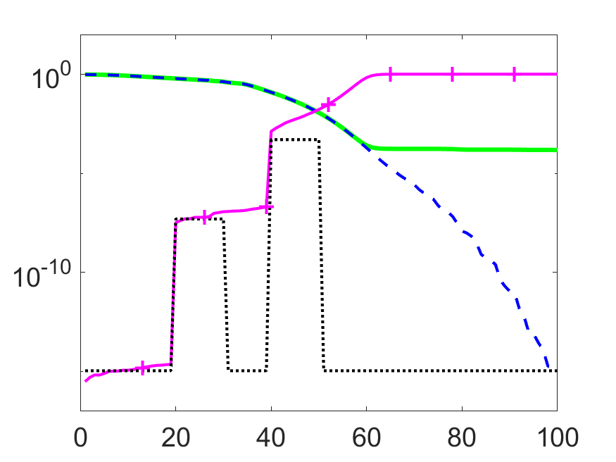
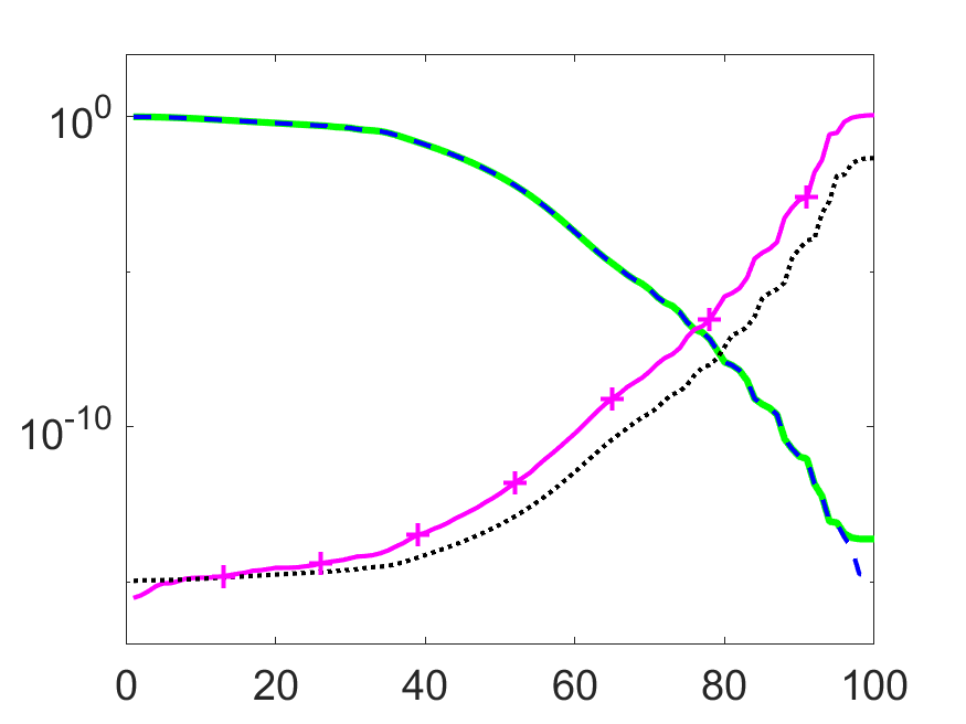
Example 1(a)	Example 1(b)

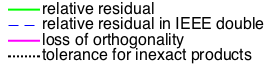
Figure 1: GMRES in variable precision: Grcar matrix.

In Example 1(a),

$$\eta_{j}=\epsilon_{j}=\begin{cases}10^{-8}\|A\|_{2},&\ \mbox{for}\ 20\leq j\leq 30,\\ 10^{-4}\|A\|_{2},&\ \mbox{for}\ 40\leq j\leq 50,\\ 2^{-52}\|A\|_{2},&\ \mbox{otherwise}.\end{cases}$$

The large increase in the inexactness of the inner products at iterations $20$ and $40$ immediately leads to a large increase in $\|F_{k}\|_{2}$. This clearly illustrates the connection between the inexactness of the inner products and the loss of orthogonality in the Arnoldi vectors. As proven in Theorem 1, until $\|F_{k}\|_{2}\approx 1$, the residual norm is the same as it would have been had all computations been performed in double precision. Due to its large increases at iterations $20$ and $40$, $\|F_{k}\|_{2}$ approaches $1$, and the residual norm starts to stagnate, long before the relative residual norm reaches the double precision machine precision.

In Example 1(b), the tolerances are chosen according to the aggressive criterion (21) with $\epsilon=2^{-52}\|A\|_{2}$. With this choice, $\|F_{k}\|_{2}$ does not reach $1$, and the residual norm does not stagnate until convergence.

5.2 Conservative vs aggressive thresholds

In our second example, $A$ is the matrix $\mathrm{494\_bus}$ from the SuiteSparse matrix collection [5]. This is a $494\times 494$ matrix with condition number $\kappa_{2}(A)\approx 10^{6}$. The right hand side is once again $b=A[\sin(1),\dots,\sin(100)]^{T}$.

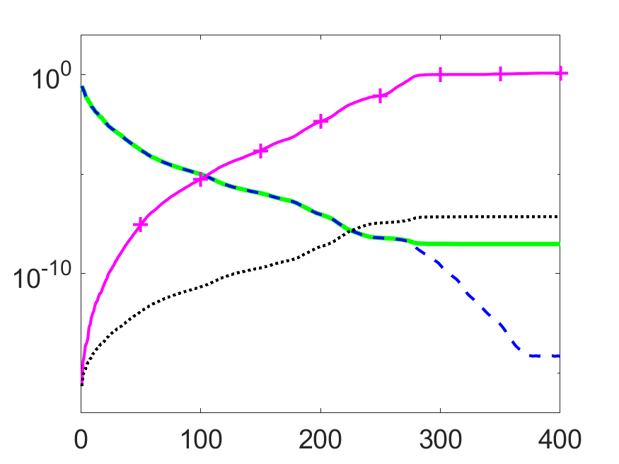
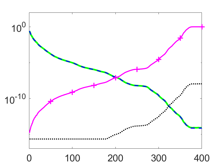
Example 2(a)	Example 2(b)

Figure 2: GMRES in variable precision: $\mathrm{494\_bus}$ matrix

Results are shown in Figure 2. In Example 2(a), tolerances are chosen according to the aggressive threshhold (21) with $\epsilon=2^{-52}\|A\|_{2}$. In this more ill-conditioned problem, the residual norm starts to stagnate before full convergence to double precision. In Example 2(b), the tolerances are chosen according to the conservative threshhold (22) with $\epsilon=2^{-52}\|A\|_{2}$, and there is no more such stagnation. Because of these lower tolerances, the inner products and matrix-vector products have to be performed in double precision until about iteration 200. This example illustrates the tradeoff between the level of inexactness and the maximum attainable accuracy. The more ill-conditioned the matrix $A$ is, the less opportunity there is for performing floating-point operations inexactly in GMRES.

6 Numerical experiments using variable floating-point arithmetic

In this section, we run variable floating-point arithmetic in order to assess the performances of the approach in the context of half, simple and double precisions. These experiments are done with the Julia language which allows to switch on demand between different floating-point types (Float16, Float32 and Float64). We compute the inner products and matrix-vector products in lower floating-point precision $u^{(low)}$ once either the aggressive threshold in (21) or the conservative threshold in (22) has increased above $u^{(low)}\|A\|_{2}$.

Compared to the previous experiments, we must now take into account the magnitudes of both the vectors and matrix perturbations in order to select the precision of the computation. When no floating-point overflow arise, the perturbation of the matrix is simply computed from the difference between the norm of the matrix stored in Float64 and its conversion to Float16 and Float32. Regarding the inner products, we estimate their magnitude based on the sum of the exponents of the two vectors involved (plus 1 for the product of the mantissa). This explains the oscillating behavior of the accuracies observed in Figures 3 and 4: even if the precision has not changed, the estimated amplitude of the value of the inner products induces changes in the associated perturbations (21) and (22).

We focus only on the $494\_\mbox{bus}$ matrix using both the conservative and agressive thresholds. The tolerances are chosen equal to $\epsilon=10^{-6}\|A\|$ and $\epsilon=10^{-12}\|A\|$ in order to illustrate the potential of the algorithm when moderate and high accuracies are required. In Figure 3, when a moderate decrease of the internally-recurred residual is required, we note that the conservative threshold results in a quick degradation of the precision for both the matrix-vector and inner products. All the matrix-vector products are computed in simple precision after 20 iterations, while the inner products start to be computed in simple precision after 30 iterations, precision that is mostly used after 90 iterations. We note a jump in the loss of orthogonality when the simple precision is triggered in the computation of the inner products. However, as expected from the theory, this does not degrade the decrease of the residual which is similar to the one observed with GMRES in double precision. When the aggressive threshold is used, we note that the simple precision is triggered after a few iterations for both the matrix-vector and inner products. The matrix-vector products are then computed in half precision from iteration 90 to convergence, while the precision of the inner products oscillate between half and single depending on the amplitude of the vectors. The consequences are a complete loss of orthogonality after 100 iterations, which results in a slowing down in the decrease of the internally-recurred residual and a stagnation of the residual.

	Conservative threshold (22)	Aggressive threshold (21)
Matrix-vector products
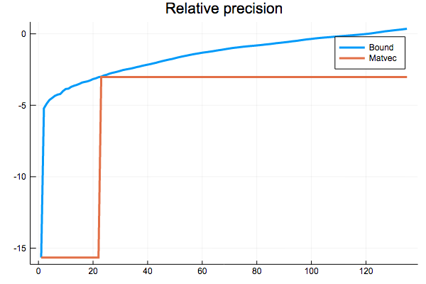
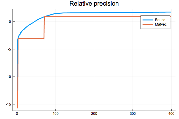
Inner products
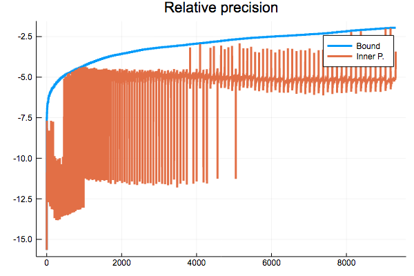
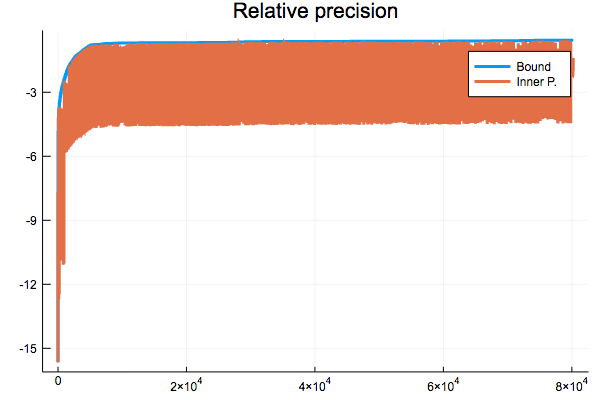
Loss of orthogonality

Double precision

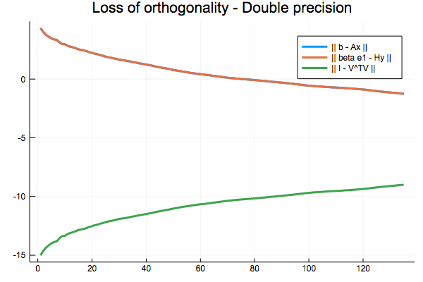
Figure 3: GMRES with variable precision floating-point arithmetic: Experiments with the $\mathrm{494\_bus}$ matrix and $\epsilon=10^{-6}\|A\|_{2}$. The bottom figure corresponds to GMRES in double precision.

The effect of requiring a higher accuracy is mainly a delay in the exploitation of the multi-arithmetic. The results shown in Figure 4 are similar to those obtained with a coarser tolerance, except for the delay in triggering the computation in simple, and half precisions. We note again a similar decrease in the residuals compared to the GMRES algorithm in double precision. The loss of orthogonality is more severe when the agressive threshold is used, due to an earlier use of the simple precision in the inner products, as well as the use of the half precision in the latest iterations. The residual does not decrease anymore until the maximum number of iterations is reached.

	Conservative threshold (22)	Aggressive threshold (21)
Matrix-vector products
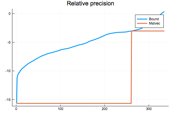
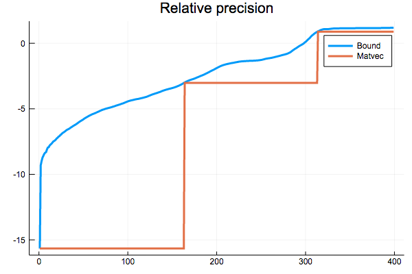
Inner products
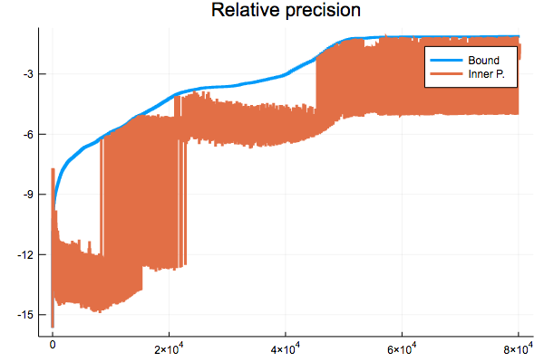
Loss of orthogonality

Double precision

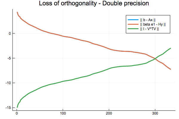
Figure 4: GMRES with variable precision floating-point arithmetic: Experiments with the $\mathrm{494\_bus}$ matrix and $\epsilon=10^{-12}\|A\|_{2}$. The bottom figure corresponds to GMRES in double precision.

This once again illustrates the tradeoff between the level of inexactness of the computations and the maximum attainable accuracy.

7 Conclusion

We have shown how inner products can be performed inexactly in MGS-GMRES without affecting the convergence or final achievable accuracy of the algorithm. We have also shown that a known framework for inexact matrix-vector products is still valid despite the loss of orthogonality in the Arnoldi vectors. It would be interesting to investigate the impact of scaling or preconditioning on these results. Additionally, in future work, we plan to address the question of how much computational savings can be achieved by this approach on massively parallel computer architectures.

Appendix A Appendix

A.1 Proof of (9)

In line 7 of Algorithm 1, in the $\ell$th pass of the inner loop at step $j$, we have

$$w_{j}^{(\ell)}=w_{j}^{(\ell-1)}-h_{\ell j}v_{\ell}$$ (30)

for $\ell=1,\dots,j$ and with $w_{j}^{(0)}=Av_{j}$. Writing this equation for $\ell=i+1$ to $j$, we have

$$w_{j}^{(i+1)} =w_{j}^{(i)}-h_{i+1,j}v_{i+1},$$

$$w_{j}^{(i+2)} =w_{j}^{(i+1)}-h_{i+2,j}v_{i+2},$$

$$\ \ \vdots$$

$$w_{j}^{(j)} =w_{j}^{(j-1)}-h_{j,j}v_{j}.$$

Summing the above and cancelling identical terms that appear on the left and right hand sides gives

$$w_{j}^{(j)}=w_{j}^{(i)}-\sum_{\ell=i+1}^{j}h_{\ell j}v_{\ell}.$$

Because $w_{j}^{(j)}=v_{j+1}h_{j+1,j}$, this reduces to

$$w_{j}^{(i)}=\sum_{\ell=i+1}^{j+1}h_{\ell j}v_{\ell}.$$ (31)

Because the inner products $h_{ij}$ are computed inexactly as in (5), from (30) we have

$$w_{j}^{(i)} =w_{j}^{(i-1)}-h_{ij}v_{i}$$

$$=w_{j}^{(i-1)}-(v_{i}^{T}w_{j}^{(i-1)}+\eta_{ij})v_{i}$$

$$=(I-v_{i}v_{i}^{T})w_{j}^{(i-1)}-\eta_{ij}v_{i}.$$

Therefore,

$$v_{i}^{T}w_{j}^{(i)}=-\eta_{ij}.$$

Multiplying (31) on the left by $-v_{i}^{T}$ gives

$$\eta_{ij}=-\sum_{\ell=i+1}^{j+1}h_{\ell j}(v_{i}^{T}v_{\ell}),$$ (32)

which is the entry in position $(i,j)$ of the matrix equation

$$\begin{bmatrix}\eta_{11}&\dots&\eta_{1k}\\ &\ddots&\vdots\\ &&\eta_{kk}\end{bmatrix}=-\begin{bmatrix}v_{1}^{T}v_{2}&\dots&v_{1}^{T}v_{k+1}\\ &\ddots&\vdots\\ &&v_{k}^{T}v_{k+1}\end{bmatrix}\begin{bmatrix}h_{21}&\dots&h_{2k}\\ &\ddots&\vdots\\ &&h_{k+1,k}\end{bmatrix},$$

i.e., (9).

A.2 Proof of Lemma 1

Equation (10) follows from

$$e_{j}^{T}H_{k}^{\dagger}\underbrace{\begin{bmatrix}H_{j-1}&0\\ 0&0\end{bmatrix}}_{\in\mathbb{R}^{(k+1)\times k}}\begin{bmatrix}y_{j-1}\\ 0_{k-j+1}\end{bmatrix}=e_{j}^{T}H_{k}^{\dagger}H_{k}\begin{bmatrix}y_{j-1}\\ 0\end{bmatrix}=e_{j}^{T}\begin{bmatrix}y_{j-1}\\ 0\end{bmatrix}=0,$$

and thus

$$|e_{j}^{T}y_{k}|=|e_{j}^{T}H_{k}^{\dagger}\beta_{1}e_{1}| =\left|e_{j}^{T}H_{k}^{\dagger}\left(\beta_{1}e_{1}-\begin{bmatrix}H_{j-1}&0\\ 0&0\end{bmatrix}\begin{bmatrix}y_{j-1}\\ 0\end{bmatrix}\right)\right|$$

$$=\left|e_{j}^{T}H_{k}^{\dagger}\begin{bmatrix}\beta_{1}e_{1}-H_{j-1}y_{j-1}\\ 0\end{bmatrix}\right|\leq\|H_{k}^{\dagger}\|_{2}\|t_{j-1}\|_{2}.$$

As for (12), for any $\gamma>0$, the smallest singular value of the matrix $\begin{bmatrix}\beta\gamma e_{1},H_{k}D_{k}^{-1}\end{bmatrix}$ is the scaled total least squares (STLS) distance [24] for the estimation problem $H_{k}D_{k}^{-1}z\approx\beta e_{1}$. As shown in [23], it can be bounded by the least squares distance

$$\min_{z}\|\beta e_{1}-H_{k}D_{k}^{-1}z\|_{2}=\|\beta e_{1}-H_{k}D_{k}^{-1}z_{k}\|_{2}=\|\beta e_{1}-H_{k}y_{k}\|_{2}=\|t_{k}\|_{2},$$

where $z_{k}=D_{k}y_{k}$. From [23, Theorem 4.1], we have

$$\frac{\|t_{k}\|_{2}}{\big{(}\gamma^{-2}+\|D_{k}y_{k}\|_{2}^{2}/(1-\tau_{k}^{2})\big{)}^{1/2}}\leq\sigma_{\min}\left(\begin{bmatrix}\beta\gamma e_{1},H_{k}D_{k}^{-1}\end{bmatrix}\right)\leq\gamma\|t_{k}\|_{2},$$ (33)

provided $\tau_{k}<1$, where

$$\tau_{k}\equiv\frac{\sigma_{\min}\left(\begin{bmatrix}\beta\gamma e_{1},H_{k}D_{k}^{-1}\end{bmatrix}\right)}{\sigma_{\min}\left(H_{k}D_{k}^{-1}\right)}.$$

We now show that if $\gamma=(\epsilon\|b\|_{2})^{-1}$ and $D_{k}$ satisfies (11), then $\tau_{k}\leq\nicefrac{{1}}{{\sqrt{2}}}$. From the upper bound in (33) we immediately have

$$\sigma_{\min}\left(\begin{bmatrix}\beta\gamma e_{1},H_{k}D_{k}^{-1}\end{bmatrix}\right)\leq\gamma\|t_{k}\|_{2}=\frac{\|t_{k}\|_{2}}{\epsilon\|b\|_{2}}.$$

Also,

$$\sigma_{\min}\left(H_{k}D_{k}^{-1}\right)=\min_{z\neq 0}\frac{\|H_{k}D_{k}^{-1}z\|_{2}}{\|z\|_{2}}=\min_{z\neq 0}\frac{\|H_{k}z\|_{2}}{\|D_{k}z\|_{2}}\geq\min_{z\neq 0}\frac{\|H_{k}z\|_{2}}{\|D_{k}\|_{2}\|z\|_{2}}=\frac{\sigma_{\min}(H_{k})}{\|D_{k}\|_{2}}.$$

Therefore, if (11) holds,

$$\tau_{k}\leq\frac{\|t_{k}\|_{2}}{\epsilon\|b\|_{2}}\frac{\|D_{k}\|_{2}}{\sigma_{\min}(H_{k})}\leq\frac{1}{\sqrt{2}}.$$

Substituting $\gamma=(\epsilon\|b\|_{2})^{-1}$ and $\tau_{k}\leq\nicefrac{{1}}{{\sqrt{2}}}$ into (33) gives (12).

A.3 Proof of Lemma 2

Note from (13) that the singular values of $Q$ satisfy

$$\big{(}\sigma_{i}(Q)\big{)}^{2}=\sigma_{i}(Q^{T}Q)=\sigma_{i}(I_{k}-F),\qquad i=1,\dots,k.$$

Therefore,

$$\sqrt{1-\|F\|_{2}}\leq\sigma_{i}(Q)\leq\sqrt{1+\|F\|_{2}},\qquad i=1,\dots,k.$$ (34)

Equation (14) is equivalent to the linear matrix equation

$$Q^{T}MQ=I_{k}-Q^{T}Q.$$

It is straightforward to verify that one matrix $M$ satisfying this equation is

$$M =(Q^{\dagger})^{T}(I_{k}-Q^{T}Q)Q^{\dagger}$$

$$=Q(Q^{T}Q)^{-1}(I_{k}-Q^{T}Q)(Q^{T}Q)^{-1}Q^{T}.$$

Notice that the above matrix $M$ is symmetric. It can also be verified using the singular value decomposition of $Q$ that the eigenvalues and singular values of $I_{n}+M$ are

$$\lambda_{i}(I_{n}+M)=\sigma_{i}(I_{n}+M)=\begin{cases}\big{(}\sigma_{i}(Q)\big{)}^{-2},&\quad i=1,\dots,k,\\ 1,&\quad i=k+1,\dots,n,\end{cases}$$

which implies that the matrix $I_{n}+M$ is positive definite. From the above and (34), provided $\|F\|_{2}\leq\delta<1$,

$$\frac{1}{1+\delta}\leq\frac{1}{\big{(}\sigma_{\max}(Q)\big{)}^{2}}\leq\sigma_{i}(I_{n}+M)\leq\frac{1}{\big{(}\sigma_{\min}(Q)\big{)}^{2}}\leq\frac{1}{1-\delta},$$ (35)

from which (15) follows.

References

• [1] A. Björck, Solving linear least squares problems by Gram-Schmidt orthogonalization, BIT Numerical Mathematics, 7 (1967), pp. 1–21.
• [2] A. Björck and C. Paige, Loss and recapture of orthogonality in the Modified Gram-Schmidt algorithm, SIAM Journal on Matrix Analysis and Applications, 13 (1992), pp. 176–190.
• [3] A. Bouras and V. Frayssé, Inexact matrix-vector products in Krylov methods for solving linear systems: A relaxation strategy, SIAM Journal on Matrix Analysis and Applications, 26 (2006), pp. 660–678.
• [4] E. Carson and N.J.Higham, Accelerating the solution of linear systems by iterative refinement in three precisions, SIAM Journal on Scientific Computing, 40 (2018), pp. 817–847.
• [5] T. A. Davis and Y. Hu, The University of Florida sparse matrix collection, ACM Transactions on Mathematical Software, 38 (2011), pp. 1–25.
• [6] J. Drkošová, A. Greenbaum, M. Rozložník, and Z. Strakoš, Numerical stability of GMRES, BIT Numerical Mathematics, 35 (1995), pp. 309–330.
• [7] J. V. D. Eshof and G. Sleijpen, Inexact Krylov subspace methods for linear systems, SIAM Journal on Matrix Analysis and Applications, 26 (2004), pp. 125–153.
• [8] R. Freund, Quasi-kernel polynomials and convergence results for quasi-minimal residual iterations, Numerical Methods in Approximation Theory, 9 (1992), pp. 77–95.
• [9] R. Freund, Quasi-kernel polynomials and their use in non-Hermitian matrix iterations, Journal of Computational and Applied Mathematics, 43 (1992), pp. 135–158.
• [10] R. Freund and N. Nachtigal, QMR: A quasi-minimal residual method for non-Hermitian linear systems, Numerische Mathematik, 60 (1991), pp. 315–339.
• [11] L. Giraud, S. Gratton, and J. Langou, Convergence in backward error of relaxed GMRES, SIAM Journal on Scientific Computing, 29 (2007), pp. 710–728.
• [12] S. Gratton, E. Simon, and P. Toint, Minimizing convex quadratic with variable precision Krylov methods, arXiv, abs/1807.07476 (2018).
• [13] A. Greenbaum, M. Rozložník, and Z. Strakoš, Numerical behaviour of the Modified Gram-Schmidt GMRES implementation, BIT Numerical Mathematics, 37 (1997), pp. 706–719.
• [14] A. Haidar, A. Abdelfattah, M. Zounon, P. Wu, S. Pradesh, S. Tomov, and J. Dongarra, The design of fast and energy-efficient linear solvers: on the potential of half-precision arithmetic and iterative refinement techniques, in Computational Science—ICCS 2018, Yong Shi, Haohuan Fu, Yingjie Tian, Valeria V. Krzhizhanovskaya, Michael Harold Lees, Jack Dongarra, and Peter M. A. Sloot editors, Springer, 2018, pp. 586–600.
• [15] A. Haidar, S. Tomov, J. Dongarra, and N. J. Higham, Harnessing GPU tensor cores for fast FP16 arithmetic to speed up mixed-precision iterative refinement solvers, in Proceedings of the International Conference for High Performance Computing, Networking, Storage, and Analysis, IEEE Press, 2018, pp. 47:1–47:11.
• [16] A. Haidar, P. Wu, S. Tomov, and J. Dongarra, Investigating half precision arithmetic to accelerate dense linear system solvers, in Proceedings of the 8th Workshop on Latest Advances in Scalable Algorithms for Large-Scale Systems, ScalA 17, 2017, pp. 10:1–10:8.
• [17] N. J. Higham, A multiprecision world, SIAM News, 50 (2017).
• [18] N. J. Higham and S. Pradesh, Simulating low precision floating-point arithmetic, SIAM Journal on Scientific Computing, 41 (2019), pp. 585–602.
• [19] N. J. Higham and S. Pradesh, Squeezing a matrix into half precision, with an application to solving linear systems, SIAM Journal on Scientific Computing, 41 (2019), pp. 2536–2551.
• [20] S. J. Leon, A. Björck, and W. Gander, Gram-Schmidt orthogonalization: 100 years and more, Numerical Linear Algebra with Applications, 20 (2013), pp. 492–532.
• [21] C. Paige, A useful form of unitary matrix obtained from any sequence of unit $2$-norm $n$-vectors, SIAM Journal on Matrix Analysis and Applications, 31 (2009), pp. 565–583.
• [22] C. Paige, M. Rozložník, and Z. Strakoš, Modified Gram-Schmidt (MGS), least squares, and backward stability of MGS-GMRES, SIAM Journal on Matrix Analysis and Applications, 28 (2006), pp. 264–284.
• [23] C. Paige and Z. Strakoš, Bounds for the least squares distance using scaled total least squares, Numerische Mathematik, 91 (2002), pp. 93–115.
• [24] C. Paige and Z. Strakoš, Scaled total least squares fundamentals, Numerische Mathematik, 91 (2002), pp. 117–146.
• [25] C. Paige and W. Wülling, Properties of a unitary matrix obtained from a sequence of normalized vectors, SIAM Journal on Matrix Analysis and Applications, 35 (2014), pp. 526–545.
• [26] J. Pestana and A. J. Wathen, On the choice of preconditioner for minimum residual methods for non-Hermitian matrices, Journal of Computational and Applied Mathematics, 249 (2013), pp. 57–68.
• [27] Y. Saad and M. H. Schultz, GMRES: A generalized minimal residual algorithm for solving nonsymmetric linear systems, SIAM Journal on Scientific and Statistical Computing, 7 (1986), pp. 856–869.
• [28] V. Simoncini and D. Szyld, Theory of inexact Krylov subspace methods and applications to scientific computing, SIAM Journal on Scientific Computing, 25 (2003), pp. 454–477.
• [29] V. Simoncini and D. Szyld, Recent computational developments in Krylov subspace methods for linear systems, Numerical Linear Algebra with Applications, 14 (2007), pp. 1–59.