MFC: An open-source high-order multi-component,
multi-phase, and multi-scale compressible flow solver

Abstract

MFC is an open-source tool for solving multi-component, multi-phase, and bubbly compressible flows. It is capable of efficiently solving a wide range of flows, including droplet atomization, shock–bubble interaction, and gas bubble cavitation. We present the 5- and 6-equation thermodynamically-consistent diffuse-interface models we use to handle such flows, which are coupled to high-order interface-capturing methods, HLL-type Riemann solvers, and TVD time-integration schemes that are capable of simulating unsteady flows with strong shocks. The numerical methods are implemented in a flexible, modular framework that is amenable to future development. The methods we employ are validated via comparisons to experimental results for shock–bubble, shock–droplet, and shock–water-cylinder interaction problems and verified to be free of spurious oscillations for material-interface advection and gas–liquid Riemann problems. For smooth solutions, such as the advection of an isentropic vortex, the methods are verified to be high-order accurate. Illustrative examples involving shock–bubble-vessel-wall and acoustic–bubble-net interactions are used to demonstrate the full capabilities of MFC.

Program summary

Title of program: MFC (Multi-component Flow Code)
Licensing provisions: GNU General Public License 3
Permanent link to code/repository: https://mfc-caltech.github.io
Operating systems under which the program has been tested: UNIX, macOS, Windows
Programming language used: Fortran 90 and Python
Nature of problem: Computer simulation of multi-component flows requires careful physical model selection and sophisticated treatment of spatial and temporal derivatives to keep solutions both thermodynamically consistent and free of spurious oscillations. Further, such methods should be high-order accurate for smooth solutions to reduce computational cost and promote sharper interfaces for discontinuous ones. These problems are particularly challenging for flows with material interfaces, which are important in numerous applications.
Solution method: The present software incorporates multiple physical models and numerical schemes for treatment of compressible multi-phase and multi-component flows. Additional physical effects and sub-grid models are included, such as an ensemble-averaged bubbly flow model. The architecture was designed to ensure that further development is straightforward.

1 Introduction

The multi-component flow code (MFC) is an open source high-order solver for multi-phase and multi-component flows. Such flows are central to a wide range of engineering problems. For example, cavitating flow phenomena are of critical importance to the development of artificial heart valves and pumps [1], minimizing injury due to blast trauma [2, 3], and improving shock- and burst-wave lithotripsy treatments [4, 5, 6]. Bubble cavitation is also pervasive in flows around hydrofoils, submarines, and high-velocity projectiles [7, 8, 9], during underwater explosions [10, 11], and within pipe systems and hydraulic machinery [12, 13]. Unfortunately, cavitation in these settings is usually detrimental, causing noise and material deterioration [13, 12]. Other cases of interest include the breakup of liquid droplets and jets [14, 15, 16], erosion of aircraft surfaces during supersonic flight [17, 18], shock-wave attenuation of nuclear blasts [19], and needle-free injection for drug delivery [20, 21].

Robust simulation of multi-component compressible flow phenomena requires a numerical method that maintains discrete conservation, suppresses oscillations near discontinuities, and preserves numerical stability. For such simulations to be computationally efficient, the method used should also be high-order accurate away from discontinuities. Schemes that can potentially achieve these requirements can be classified as either interface-tracking or interface-capturing [22]. Examples of interface-tracking methods include free-Lagrange [23, 24], front-tracking [25, 26], and level-set/ghost fluid schemes [27, 28, 29, 30, 31, 32, 33]; these methods differ from interface-capturing as they treat material interfaces as sharp features in the flow. This allows interfacial fluids to have differing equations of state and ensures that interfacial physics are straightforward to implement. Unfortunately, they do not naturally enforce discrete or total conservation, though there have been some recent attempts to partially include these properties [34, 35]. Interface-capturing methods instead treat interfaces as discontinuities in material properties via advected volume fractions. Such methods are generally more efficient than interface-tracking schemes [36] and can achieve discrete conservation by simply solving the governing equations in conservative form. However, they also smear material interfaces via numerical diffusion [37, 38, 39]. In these smeared regions, we must ensure that the mixture properties are treated in a thermodynamically- and numerically-consistent way, such that spurious oscillations (and other physical inconsistencies) are avoided in the presence of high density contrasts between materials. Fortunately, such methods have been developed and prove to be a robust treatment of interfacial dynamics [40, 37, 41]. Still, the lack of a coherent material interface means that interfacial physics are more challenging to implement than interface-tracking methods, though conservative treatments do exist for both interfacial heat transfer [42] and capillary effects [38, 43, 16].

Here, we choose to use an interface-capturing scheme because computational efficiency and discrete conservation are of principal importance to many problems of interest. The interface-capturing schemes we use follow from the so-called 5- and 6-equation models, which are known to be sufficient for representing a wide range of flow phenomenologies [42, 44, 45, 46]. They are complemented by a discretely-conservative numerical method that solves the conservative form of the compressible flow equations. To maintain a non-oscillatory behavior near material interfaces, the material advection equations are formulated in a quasi-conservative form [47]. The equations of motion are then closed by a thermodynamically consistent set of mixture rules [44]. The governing equations are solved with a shock-capturing finite-volume method. Specifically, we adopt a WENO spatial reconstruction that can achieve high-order accuracy while maintaining non-oscillatory behavior near material interfaces [48, 49, 50, 41]. This scheme is then coupled with an HLL-type approximate Riemann solver [51, 52] and a total-variation-diminishing (TVD) time stepper [53].

MFC is, of course, not the only viable option for simulation of compressible multi-phase flows. For example, ECOGEN [54] offers a pressure-disequilibrium-based interface-capturing scheme that is well suited for the same problems reached by MFC. However, ECOGEN is built upon an intrinsically low-order MUSCL scheme that can inhibit both efficient simulation and physically fidelity when compared to the WENO schemes we use here, especially when augmented with our high-order cell-average approximations. This is demonstrated in section 5.4 for an isentropic vortex problem and in section 5.3 and Schmidmayer et al. [55] for cavitating gas bubbles. In pursuit of this, MFC was also constructed with a phase-averaged flow model that represent unresolved multi-phase dynamics at the sub-grid level. More mature CFD solvers such as OpenFOAM are also available. OpenFOAM natively supports finite-volume methods for multi-component flows [56], though higher-order methods and interface-capturing models are only available via links to external forked projects. MFC instead offers an integrated approach that avoids any conflicts from such libraries. Finally, the parallel I/O file systems we employ ensures that the MFC architecture can scale up to the largest modern HPC systems.

Herein, we describe version 1.0 of MFC. In section 2 we present an overview of what is included in the MFC package, including its organization, features, and logistics. The physical models we use are presented in section 3, including the associated mixture rules, governing equations, equations of state, and our implementation of an ensemble-averaged bubbly flow model. The numerical methods used to solve the associated equations are presented in section 4. A series of test cases simulated using MFC are discussed in section 5; these verify and validate our method. These are complemented by a set of illustrative example cases that further demonstrate MFC’s capabilities in section 6 and parallel benchmarking in section 7, which analyzes the performance of MFC on large scale computing clusters. Section 8 concludes our presentation of MFC.

2 Overview and features

2.1 Package, installation, and testing

MFC is available at https://mfc-caltech.github.io. The source code is written using Fortran 90 with MPI bindings used for parallel communication and Python scripts are used to generate input files. Installation of MFC requires the FFTW package for cylindrical coordinate treatment [57], and, optionally, Silo and its dependencies for post-treatment of data files [58]. We only provide the FFTW package with MFC to keep the package relatively small.

Name	Description
example_cases/	Example and demonstration cases
doc/	Documentation
installers/	Package installers: Includes FFTW
lib/	Libraries
src/	Source code
master_scripts/	Python modules and dictionaries, optional source files
pre_process_code/	Generates initial conditions and grids
simulation_code/	Flow solver
post_process_code/	Processes simulation data
tests/	Test cases to ensure software is operating as intended
AUTHORS	List of contributors and their contact information
CONFIGURE	Package configuration guide
COPYRIGHT	Copyright notice
INSTALL	Installation guide
LICENSE	The GNU public license file
Makefile.in	Makefile input; generally does not need to be modified
Makefile.user	User inputs for compilation; requires attention from user
Makefile	Targets: all (default), [component], test, clean
RELEASE	Release notes

Table 1: Descriptions of the files and directories included in MFC. [component] is one of pre_process, simulation, or post_process.

The MFC package includes several directories; their organization and descriptions are shown in table 1. New users should consult the CONFIGURE and INSTALL files for instructions on how to compile MFC. In brief, the user must ensure that Python and an MPI Fortran compiler are loaded and that the FFTW package can be located by Makefile; this can be done by pointing Makefile.user to the correct location or by installing the included FFTW distribution in the installers directory. Once the software has been built, the test target of Makefile should be called; it runs multiple tests (which are located in the tests directory) to ensure that MFC is operating as intended.

2.2 Features

MFC uses a fully parallel environment via message passing interfaces (MPI), the performance of which is the subject of section 7. Computationally, it includes structured Cartesian and cylindrical grids with non-uniform mesh stretching available; characteristic-based Thompson, periodic, and free-slip boundary conditions have also been implemented. The 5- and 6-equation flow models can be used with a flexible number of components, as discussed in section 3. Ensemble-averaged dilute bubbly flow modeling is also available, including options for Gilmore and Keller–Miksis single-bubble models (see section 3.3). The numerical methods are discussed in section 4; they include 1-, 3-, and 5-th order accurate WENO reconstructions on optionally the primitive, conservative, or characteristic variables. Within each finite volume, high-order evaluation is available for the cell-averaged variables via Gaussian quadrature for multi-dimensional problems. The shock-capturing schemes are paired with either HLL, HLLC, or exact Riemann solvers. For time-stepping, 1–5-th order accurate Runge–Kutta methods are available. These features will, of course, evolve and expand with time.

Of great practical importance are the user interfaces we utilize. MFC features Python input scripts, which operate via dictionaries to automatically write input files that are read via Fortran namelists. Additionally, the file system and data formats were selected to enable large-scale parallel simulations. Specifically, we use the Lustre file system to generate and read restart files; it can support gigabyte-per-second-scale IO operations and petabyte-scale storage requirements [59], which ensures that the MFC can utilize the full capabilities of modern HPC systems. We also utilize HDF5 Silo databases, which keeps the file structure compact and enables parallel visualization. We have confirmed that MFC works as expected on various high-performance computing platforms, including modern SGI- and Dell-based supercomputers.

2.3 Software structure

2.3.1 Pre-processing

The pre-processor generates initial conditions and spatial grids from the physical patches specified in the Python input file and exports them as binary files to be read by the simulator. Specifically, this involves allocating and writing either a Cartesian or cylindrical mesh, with the option of mesh stretching, according to the input parameters. The specified physical variables for each patch are transformed into their conservative form and written in a manner consistent with the mesh. The pre-processor is comprised of individual Fortran modules that read input values and export mesh and initial condition files, assign then distribute global variables via MPI, perform variable transformations, generate grids, parse and assign patch types, and check that specified input variables are physically consistent and that specified options do not contradict each other.

2.3.2 Simulation

The simulator, given the initial-condition files generated by the pre-processor, solves the corresponding governing flow equations with the specified boundary conditions using our interface-capturing numerical method. Simulations are conducted for the number of time steps indicated. The simulator exports run-time information, restart files that can be used to either restart the simulation or post-process the associated data, and, optionally, human-readable output data. The structure of the simulator follows that of pre-processor, with individual Fortran modules conducting each software component; this includes reading and exporting data and grid files, performing Fourier transforms, assigning and distributing global variables via MPI, performing variable transformations, computing time and spatial derivatives using WENO and the Riemann solver specified, computing boundary values, including ensemble-averaged bubbly flow physics, and checking that the input variables are valid.

2.3.3 Post-processing

The post-processor reads simulation data and exports HDF5/Silo databases that include variables and derived variables, as specified in the input file. Since the simulator can export human-readable data, post-processing is not essential for the usage of MFC, but is a useful tool, especially for large or parallel data structures. Specifically, the post-process component of the MFC reads the restart files exported by the simulator at distinct time intervals and computes the necessary derived quantities. The HDF5 database is then generated and exported, and can be readily viewed using, for example, VisIt [60] or Paraview [61]. Again, individual Fortran modules perform the associated tasks, including reading data, parameter conversion, assigning and distributing global MPI variables, computing Fourier transforms, exporting HDF5 Silo databases, and checking that the input parameters are consistent.

2.4 Description of input/output files

	Name	Description
Input	input.py	Input parameters
	pre_process.inp	Pre-process input parameters, auto-generated
	simulation.inp	Simulation input parameters, auto-generated
	post_process.inp	Post-process input parameters, auto-generated
Output	run_time.inf	Run-time information including current simulation time and CFL
	D/	Formatted simulation output files
	p_all/	Binary simulation restart files (depending upon options used)
	restart_data/	Lustre restart files (depending upon options used)
	silo_HDF5/	Silo post-process files (depending upon options used)
	binary/	Binary post-process files (depending upon options used)

Table 2: Input/output files in the case-specific directory.

We next describe the contents of a case-specific directory and its logistics. The specific file structure is shown in table 2. The Python script input.py is used to generate the input files (*.inp) for the source codes and execute an MFC component (one of pre_process, simulation, or post_process) either in the active window or as a submitted batch script. This Python file contains the input parameters available for the MFC. MFC, depending upon the component used and options selected, will generate several files and directories. If enabled, the run_time.inf file will be generated by the simulator and includes details about the current time step, simulation time, and stability criterion. Directories that contain binary restart data and output files for visualization or further post-treatment are generated, again depending upon the specified options, by the simulator and post-processor.

3 Physical model and governing equations

The mechanical-equilibrium compressible multi-component flow models we use can be written as

$$\frac{\partial\bm{q}}{\partial t}+\nabla\cdot\bm{F}\left(\bm{q}\right)+\bm{h}\left(\bm{q}\right)\nabla\cdot\bm{u}=\bm{s}\left(\bm{q}\right),$$ (1)

where $\bm{q}$ is the state vector, $\bm{F}$ is the flux tensor, $\bm{u}$ is the velocity field, and $\bm{h}$ and $\bm{s}$ are non-conservative quantities we describe subsequently.

3.1 5-equation model

We first introduce our implementation of the thermodynamically consistent mechanical-equilibrium model of Kapila et al. [45]. Our multi-component implementation can be used for $N_{k}$ components, though we present a two-component ($N_{k}=2$) configuration here for demonstration purposes. It consists of five partial differential equations as

$$\bm{q}=\left[\begin{array}[]{c}\alpha_{1}\\ \alpha_{1}\rho_{1}\\ \alpha_{2}\rho_{2}\\ \rho\bm{u}\\ \rho E\end{array}\right],\quad\bm{F}=\left[\begin{array}[]{c}\alpha_{1}\bm{u}\\ \alpha_{1}\rho_{1}\bm{u}\\ \alpha_{2}\rho_{2}\bm{u}\\ \rho\bm{u}\otimes\bm{u}+p\bm{I}-\bm{T}\\ \left(\rho E+p\right)\bm{u}-\bm{T}\cdot\bm{u}\end{array}\right],\quad\bm{h}=\left[\begin{array}[]{c}-\alpha_{1}-K\\ 0\\ 0\\ \mathbf{0}\\ 0\end{array}\right],\quad\bm{s}=\mathbf{0},$$ (17)

where $\rho$, $\bm{u}$, and $p$ are the mixture density, velocity, and pressure, respectively, $\alpha_{k}$ is the volume fraction of component $k$, and $\bm{T}$ is the viscous stress tensor

$$\bm{T}=2\eta\left(\bm{D}-\frac{1}{3}(\nabla\cdot\bm{u})\bm{I}\right),$$ (18)

where $\eta$ is the mixture shear viscosity and

$$\bm{D}=\frac{1}{2}\left(\nabla\bm{u}+(\nabla\bm{u})^{\top}\right)$$ (19)

is the strain rate tensor. The mixture total and internal energies are $E=e+\|\bm{u}\|^{2}/2$ and

$$e=\sum_{k=1}^{N_{k}}Y_{k}e_{k}\left(\rho_{k},p\right),$$ (20)

respectively, where $Y_{k}=\alpha_{k}\rho_{k}/\rho$ are the mass fractions of each component. We close (20) using the stiffened-gas equation of state, which is chosen for its ability to faithfully model both liquids and gases [62]; for component $k$ it is

$$p_{k}=(\gamma_{k}-1)\rho_{k}e_{k}-\gamma_{k}\pi_{\infty,k},$$ (21)

where $\gamma$ is the specific heat ratio and $\pi_{\infty}$ is the liquid stiffness (gases have $\pi_{\infty}=0$) [63]. For liquids, these are usually interpreted as fitted parameters from shockwave-Hugoniot data [64, 65]. The speed of sound of each component is then

$$c_{k}=\sqrt{\frac{\gamma_{k}(p_{k}+\pi_{\infty,k})}{\rho_{k}}}.$$ (22)

The $K$ term in $\bm{h}$ of (17) represents expansion and compression in mixture regions. For an $N_{k}=2$ configuration it is

$$K=\frac{\rho_{2}c_{2}^{2}-\rho_{1}c_{1}^{2}}{\frac{\rho_{2}c_{2}^{2}}{\alpha_{2}}+\frac{\rho_{1}c_{1}^{2}}{\alpha_{1}}}$$ (23)

and the mixture speed of sound $c$ follows as the so-called Wood speed of sound [66, 67]

$$\frac{1}{\rho c^{2}}=\sum_{k=1}^{N_{k}}\frac{\alpha_{k}}{\rho_{k}c_{k}^{2}}.$$ (24)

Ultimately, the equations are closed by the usual set of mixture rules

$$1=\sum_{k=1}^{N_{k}}\alpha_{k},\quad\rho=\sum_{k=1}^{N_{k}}\alpha_{k}\rho_{k},\quad\rho e=\sum_{k=1}^{N_{k}}\alpha_{k}\rho_{k}e_{k},\quad\text{and}\quad\eta=\sum_{k=1}^{N_{k}}\alpha_{k}\eta_{k}.$$ (25)

We note that the models of Allaire et al. [44] and Massoni et al. [42] do not include the $K$ term in (17) and thus do not strictly obey the second-law of thermodynamics, nor reproduce the correct mixture speed of sound (24). While MFC also supports these models, accurately representing the sound speed is known to be important for some problems, such as the cavitation of gas bubbles [55]. However, it is also known that the $K$ term can result in numerical instabilities for problems with strong compression or expansion in mixture regions due to its non-conservative nature [55]. Thus, the decision of what 5-equation model to use (if any) is problem dependent and left to the user.

3.2 6-equation model

While the 5-equation model described in section 3.1 is efficient and represents the correct physics, the $K\nabla\cdot\bm{u}$ term that makes the model thermodynamically consistent can sometimes introduce numerical instabilities [46, 55]. In such cases, a pressure-disequilibrium is preferable [55]. We also support the 6-equation pressure-disequilibrium model of Saurel et al. [46], which for a two-component configuration is expressed as

$$\bm{q}=\left[\begin{array}[]{c}\alpha_{1}\\ \alpha_{1}\rho_{1}\\ \alpha_{2}\rho_{2}\\ \rho\bm{u}\\ \alpha_{1}\rho_{1}e_{1}\\ \alpha_{2}\rho_{2}e_{2}\end{array}\right],\quad\bm{F}=\left[\begin{array}[]{c}\alpha_{1}\bm{u}\\ \alpha_{1}\rho_{1}\bm{u}\\ \alpha_{2}\rho_{2}\bm{u}\\ \rho\bm{u}\otimes\bm{u}+p\bm{I}-\bm{T}\\ \alpha_{1}\rho_{1}e_{1}\bm{u}\\ \alpha_{2}\rho_{2}e_{2}\bm{u}\end{array}\right],\quad\bm{h}=\left[\begin{array}[]{c}-\alpha_{1}\\ 0\\ 0\\ \mathbf{0}\\ \alpha_{1}p_{1}\\ \alpha_{2}p_{2}\end{array}\right],\quad\bm{s}=\left[\begin{array}[]{c}\mu\delta p\\ 0\\ 0\\ \mathbf{0}\\ -\mu p_{I}\delta p-\alpha_{1}\bm{T}_{1}:\nabla\bm{u}\\ \phantom{-}\mu p_{I}\delta p-\alpha_{2}\bm{T}_{2}:\nabla\bm{u}\end{array}\right],$$ (50)

where $\bm{T}_{k}$ are the component-specific viscous stress tensors and the other terms of $\bm{s}$ represent the relaxation of pressures between components with coefficient $\mu$. The interfacial pressure is

$$p_{I}=\frac{z_{2}p_{1}+z_{1}p_{2}}{z_{1}+z_{2}},$$ (51)

where $z_{k}=\rho_{k}c_{k}$ is the acoustic impedance of component $k$ and

$$\delta p=p_{1}-p_{2},$$ (52)

is the pressure difference. Since $p_{1}\neq p_{2}$, the total energy equation of the mixture is replaced by the internal-energy equation for each component. The mixture speed of sound is defined according to

$$c^{2}=\sum_{k=1}^{2}Y_{k}c_{k}^{2},$$ (53)

though after applying the numerical infinite pressure-relaxation procedure detailed in section 4.6 the effective mixture speed of sound matches (24).

3.3 Bubbly flow model

3.3.1 Implementation

MFC includes support for the ensemble-phase-averaged bubbly flow model of Zhang and Prosperetti [68], and our implementation of it matches that of Bryngelson et al. [69]. The bubble population has void fraction $\alpha_{b}$, which is assumed to be small, and the carrier components have mixture pressure $p_{l}$. The equilibrium radii of the bubble population are represented discretely as $\bm{R}_{o}$, which are $N_{\text{bin}}$ bins of an assumed log-normal PDF with standard deviation $\sigma_{p}$ [70]. The instantaneous bubble radii are a function of these equilibrium states as $\bm{R}(\bm{R}_{o})=\{R_{1},R_{2},\dots,R_{N_{\text{bin}}}\}$. The total mixture pressure is modified as

$$p=(1-\alpha_{b})p_{l}+\alpha_{b}\left(\frac{\mkern 1.5mu\overline{\mkern-1.5mu\bm{R}^{3}\bm{p}_{bw}\mkern-1.5mu}\mkern 1.5mu}{\mkern 1.5mu\overline{\mkern-1.5mu\bm{R}^{3}\mkern-1.5mu}\mkern 1.5mu}-\rho\frac{\mkern 1.5mu\overline{\mkern-1.5mu\bm{R}^{3}\dot{\bm{R}}^{2}\mkern-1.5mu}\mkern 1.5mu}{\mkern 1.5mu\overline{\mkern-1.5mu\bm{R}^{3}\mkern-1.5mu}\mkern 1.5mu}\right),$$ (54)

where $\dot{\bm{R}}$ are the bubble radial velocities and $\bm{p}_{bw}$ are the bubble wall pressures. Overbars $\mkern 1.5mu\overline{\mkern-1.5mu\cdot\mkern-1.5mu}\mkern 1.5mu$ denote the usual moments with respect to the log-normal PDF. The bubble void fraction is advected as

$$\frac{\partial\alpha_{b}}{\partial t}+\bm{u}\cdot\nabla\alpha_{b}=3\alpha_{b}\frac{\mkern 1.5mu\overline{\mkern-1.5mu\bm{R}^{2}\dot{\bm{R}}\mkern-1.5mu}\mkern 1.5mu}{\mkern 1.5mu\overline{\mkern-1.5mu\bm{R}^{3}\mkern-1.5mu}\mkern 1.5mu},$$ (55)

and the bubble dynamic variables are evolved as

$$\frac{\partial n\boldsymbol{\phi}}{\partial t}+\nabla\cdot(n\boldsymbol{\phi}\bm{u})=n\dot{\boldsymbol{\phi}},$$ (56)

where $\boldsymbol{\phi}\equiv\left\{\bm{R},\dot{\bm{R}},\bm{p}_{b},\bm{m}_{v}\right\}$ (see section 3.3.2) and $n$ is the conserved bubble number density per unit volume

$$n=\frac{3}{4\pi}\frac{\alpha_{b}}{\mkern 1.5mu\overline{\mkern-1.5mu\bm{R}^{3}\mkern-1.5mu}\mkern 1.5mu}.$$ (57)

3.3.2 Single-bubble dynamics

A partial differential equation following (56) is evolved for each bin representing equilibrium radius $R_{o}$. These equations assume that each bubble evolves, without interaction with its neighbors, in an otherwise uniform flow whose properties are dictated by the local mixture-averaged flow quantities [71]. We also assume that the bubbles remain spherical, maintain a uniform internal pressure, and do not break-up, or coalesce. Our model includes the thermal effects, viscous and acoustic damping, and phase change. The bubble radial accelerations $\ddot{R}$ are computed by the Keller–Miksis equation [72]:

$$R\ddot{R}\left(1-\frac{\dot{R}}{c_{b}}\right)+\frac{3}{2}\dot{R}^{2}\left(1-\frac{\dot{R}}{3c_{b}}\right)=\frac{p_{bw}-p_{l}}{\rho}\left(1+\frac{\dot{R}}{c_{b}}\right)+\frac{R\dot{p}_{bw}}{\rho c_{b}},$$ (58)

where $c_{b}$ is the usual speed of sound associated with the bubble and

$$p_{bw}=p_{b}-\frac{4\mu\dot{R}}{R}-\frac{2\sigma}{R}$$ (59)

is the bubble wall pressure, for which $p_{b}$ is the internal bubble pressure, $\sigma$ is the surface tension coefficient, and $\mu$ is the liquid viscosity. The evolution of $p_{b}$ is evaluated using the model of Ando [71]:

$$\dot{p}_{b}=\frac{3\gamma_{b}}{R}\left(\mathfrak{R}_{v}T_{bw}\dot{m}_{v}-\dot{R}p_{b}+\frac{\gamma_{b}-1}{\gamma_{b}}\lambda_{bw}\left.\frac{\partial T}{\partial r}\right|_{r=w}\right),$$ (60)

where $T$ is the temperature, $\lambda$ is the thermal conductivity, $\mathfrak{R}_{v}$ is the gas constant and $\gamma_{b}$ is the specific heat ratio of the gas. Mass transfer of the bubble contents follows the reduced model of Preston et al. [73] as

$$\dot{m}_{v}=\frac{\mathcal{D}\rho_{bw}}{1-\chi_{vw}}\left.\frac{\partial\chi_{v}}{\partial r}\right|_{w}.$$ (61)

4 Solution method

Our numerical scheme generally follows that of Coralic and Colonius [41]. The spatial discretization of (1) in three-dimensional Cartesian coordinates is

$$\frac{\partial\bm{q}}{\partial t}+\frac{\bm{F}^{x}(\bm{q})}{\partial x}+\frac{\bm{F}^{y}(\bm{q})}{\partial y}+\frac{\bm{F}^{z}(\bm{q})}{\partial z}=\bm{s}(\bm{q})-\bm{h}(\bm{q})\nabla\cdot\bm{u},$$ (62)

where $\bm{F}^{x_{i}}$ are the $i\in(x,y,z)$-direction flux vectors and the treatment of $\nabla\cdot\bm{u}$ is discussed later.

4.1 Treatment of spatial derivatives

We use a finite volume method to treat the spatial derivatives of (62). The finite volumes are

$$I_{i,j,k}=[x_{i-1/2},x_{i+1/2}]\times[y_{j-1/2},y_{j+1/2}]\times[z_{k-1/2},z_{k+1/2}].$$ (63)

We spatially integrate (62) within each cell-centered finite volume as

$$\begin{split}\frac{\text{d}\bm{q}_{i,j,k}}{\text{d}t}=&\frac{1}{\Delta x_{i}}[\bm{F}_{i-1/2,j,k}^{x}-\bm{F}_{i+1/2,j,k}^{x}]+\\ &\frac{1}{\Delta y_{j}}[\bm{F}_{i,j-1/2,k}^{y}-\bm{F}_{i,j+1/2,k}^{y}]+\\ &\frac{1}{\Delta z_{k}}[\bm{F}_{i,j,k-1/2}^{z}-\bm{F}_{i,j,k+1/2}^{z}]+\bm{s}(\bm{q}_{i,j,k})-\bm{h}(\bm{q}_{i,j,k})(\nabla\cdot\bm{u})_{i,j,k},\end{split}$$ (64)

where

$$\bm{q}_{i,j,k}=\frac{1}{V_{i,j,k}}\iiint_{I_{i,j,k}}\bm{q}(x,y,z,t)\,\text{d}x\text{d}y\text{d}z,$$ (65)

$$\bm{s}_{i,j,k}=\frac{1}{V_{i,j,k}}\iiint_{I_{i,j,k}}\bm{s}(x,y,z,t)\,\text{d}x\text{d}y\text{d}z,$$ (66)

$$\bm{F}_{i+1/2,j,k}=\frac{1}{\Delta y_{j}\Delta z_{k}}\iint_{A_{i+1/2,j,k}}\bm{F}(x,y,z,t)\,\text{d}y\text{d}z,$$ (67)

are cell-volume and face averages, for which $\Delta x_{i}=x_{i+1/2}-x_{i-1/2}$ are the mesh spacings ($\Delta y$ and $\Delta z$ have the same form), and $V_{i,j,k}$ and $A_{i+1/2,j,k}$ are the cell volumes and face areas.

MFC can approximate this equation using high-order quadratures as opposed to simple cell-centered averages. This approach computes the flux surface integrals and source terms using a two-point, fourth-order, Gaussian quadrature rule, e.g.

$$\bm{F}_{i+1/2,j,k}=\frac{1}{4}\sum_{m=1}^{2}\sum_{l=1}^{2}\bm{F}(\bm{q}(x_{i+1/2},y_{j_{l}},z_{k_{m}})),$$ (68)

where $l$ and $m$ are the Gaussian quadrature point indices and

$$y_{j_{l}}=y_{j}+(2l+1)\frac{\Delta y_{j}}{2\sqrt{3}}\quad\text{and}\quad z_{k_{m}}=z_{k}+(2m+1)\frac{\Delta z_{k}}{2\sqrt{3}}.$$ (69)

The divergence terms are treated using a midpoint rule

$$\begin{split}(\nabla\cdot&\bm{u})_{i,j,k}=\\ &\frac{1}{\Delta x_{i}}(u_{i+1/2,j,k}-u_{i-1/2,j,k})+\frac{1}{\Delta y_{j}}(v_{i,j+1/2,k}-v_{i,j-1/2,k})+\frac{1}{\Delta z_{k}}(w_{i,j,k+1/2}-w_{i,j,k-1/2}),\end{split}$$ (70)

where $\bm{u}=\{u,v,w\}$ are the cell-averaged velocity components computed analogous to (68).

To avoid spurious oscillations at material interfaces, we ultimately evaluate the fluxes by reconstructing the primitive or characteristic variables at the cell faces via a 5th-order-accurate WENO scheme [41] (though reconstruction of the conservative variables and lower-order WENO schemes are also supported). This allows us to apply a Riemann solver, so

$$\bm{F}_{i+1/2,j,k}=\frac{1}{4}\sum_{m=1}^{2}\sum_{l=1}^{2}\widehat{\bm{F}}(\bm{q}_{i+1/2,j,k}^{L},\bm{q}_{i+1/2,j,k}^{R}),$$ (71)

where $\widehat{\bm{F}}$ is the numerical flux function of the Riemann solver. We use the HLLC approximate Riemann solver to compute the fluxes [52], though other Riemann solvers are also supported.

4.2 Limiters for improved numerical stability

4.2.1 Volume fraction limiting

Following our mixture rules (25), the volume fractions are physically required to sum to unity. However, the accumulation of numerical errors can preclude this if the first $N_{k}-1$ volume fractions exceed unity, and thus one of the volume fractions must be negative [74]. This is of course unphysical and leads to other numerical issues, such as complex speeds of sound. To treat this, we impose the volume fraction mixture rule by limiting each volume fraction as $0\leq\alpha_{k}\leq 1$ for all components $k$, then rescaling them as

$$\alpha_{k}=\frac{\alpha_{k}}{\sum_{k=1}^{N_{k}}\alpha_{k}}\quad\text{for}\;k=1,\dots,N_{k}.$$ (72)

We note that we only use this limiting when computing the mixture properties, and do not alter them otherwise as to avoid polluting the mass conservation properties of the method.

4.2.2 Flux limiting

The WENO schemes we utilize are, in general, not TVD. This can be problematic when WENO cannot form a smooth stencil to reconstruct, and can lead to numerical instabilities even when the usual CFL criteria are met. MFC supports advective flux limiting to treat this issue, which improves stability, though it also increases numerical dissipation and thus smearing of material interfaces. However, we use the gradient of the local volume fraction $\chi$ to minimize this effect, which localizes the limiter to non-smooth regions of the flow. In one dimension of our dimensional-splitting procedure this yields

$$\chi_{i}=\begin{dcases*}\frac{\alpha_{i}-\alpha_{i-1}}{\alpha_{i+1}-\alpha_{i}}&if $u^{*}\geq 0$,\\ \frac{\alpha_{i+2}-\alpha_{i+1}}{\alpha_{i+1}-\alpha_{i}}&if $u^{*}<0$,\end{dcases*}$$ (73)

where $i$ is the spatial index and $u^{*}$ is the local velocity computed by the Riemann solver. Ultimately, the modified flux is a combination of a low- and high-order accurate flux approximation. The low-order flux is chosen to be equivalent to a first-order WENO reconstruction and the high-order flux is the Riemann flux from the WENO reconstruction. Specifically, MFC supports the minmod, MC, ospre, superbee, Sweby, van Albada, or van Leer flux limiters, each of which is a function of the volume fraction gradient $\chi$. Further details of our numerical implementation are located in Meng [74].

4.3 Cylindrical coordinate considerations

MFC also supports the use of cylindrical coordinates. They are formulated in similar fashion to (62), though with the addition of an additional set of source terms on the right-hand-side associated with the $1/r$ cylindrical terms of the divergence operator. Our implementation was detailed by Meng [74] and does not use an alternative treatment of the WENO weights in the azimuthal direction, such as would be required to ensure high-order accuracy away from discontinuities. While such methods for this exist, they are generally complex and suffer from numerical stability issues [75, 76, 77]. The cylindrical coordinate treatment also requires velocity gradients, rather than just velocities, at cell boundaries. For this, we use a second-order-accurate finite-difference and averaging procedure to obtain the necessary velocity gradients at these points. Finally, the coordinate singularity at $r\to 0$ is treated using the method of Mohseni and Colonius [78], which performs differentiation in the radial direction via a redefinition of the radial coordinate; in our implementation, we place the singularity at the finite-volume cell boundary (rather than the center). We note that this implementation requires an even number of grid cells in the azimuthal coordinate direction. A consequence of the cylindrical coordinate system is that the grid cells near the radial center are much smaller than those far away, which restricts the global CFL criterion. Following Mohseni and Colonius [78], we address this issue by using a spectral filter, which filters the high-frequency components of the solution near the centerline and relaxes the CFL criterion. Our implementation was verified by Meng [74] to be second-order accurate away from discontinuities via a propagating spherical pressure pulse, while the construction of the viscous stress tensor was verified using the method of manufactured solutions.

4.4 One-way acoustic wave generation

The source term $\bm{s}$ of (1) and (62) can be augmented with additional terms $\bm{s}^{s}(t)$ for the generation of one-way acoustic waves, for examples to model an ultrasound transducer immersed in the flow. Following Maeda and Colonius [79], these take the form

$$\bm{s}^{s}(t)=\int_{\Gamma}\Omega_{\Gamma}(\boldsymbol{\xi},t)\delta(\bm{X}(\boldsymbol{\xi},t)-\bm{x})\text{d}\boldsymbol{\xi}$$ (74)

where $\Omega_{\Gamma}$ is (possibly time dependent) forcing, $\Gamma$ is the surface the forcing acts upon, $\delta$ is the Dirac delta function, and $\bm{X}$ maps the $\boldsymbol{\xi}$ coordinate to physical space $\bm{x}$. In our numerical framework this is represented at cell $I_{i,j,k}$ as

$$\bm{s}_{i,j,k}^{s}(t)=\sum_{m=1}^{M}\Omega_{\Gamma}(\xi_{m},t)\delta_{h}(|\bm{X}(\xi_{m},t)-\bm{x}_{i,j,k}|)\Delta\xi_{m},$$ (75)

where $\delta_{h}$ is the discrete delta function operator, $\Delta\xi_{k}$ are the sizes of the discrete patch or line the forcing is applied to, and $M$ are the number of such patches. For example, in two dimensions the one-dimensional line operator follows as

$$\delta_{h}(h)=\frac{1}{2\pi\sigma^{2}}e^{-\frac{1}{2}\frac{h^{2}}{\sigma^{2}}},$$ (76)

where $\sigma=3\Delta$ and $\Delta$ is the largest mesh spacing. For a single-component, two-dimensional problem (note that there is no volume-fraction advection equation in this case) the forcing is expressed as

$$\Omega_{\Gamma}(t)=f(t)[1/c_{o},\cos(\theta),\sin(\theta),c_{o}^{2}/(\gamma-1)],$$ (77)

where $f(t)$ is the time-dependent pulse amplitude, $c_{o}$ is the speed of sound, and $\theta$ is the forcing direction as measured from the first-coordinate axis.

4.5 Time integration

Once the spatial derivatives have been approximated, (62) becomes a semi-discrete system of ordinary differential equations in time. We treat the temporal derivative using a Runge–Kutta time-marching scheme for the state variables. To achieve high-order accuracy and avoid spurious oscillations, we use the third-order-accurate total variation diminishing scheme of Gottlieb and Shu [53]:

$$\bm{q}_{i,j,k}^{(1)} =\bm{q}_{i,j,k}^{n}+\Delta t\bm{L}(\bm{q}_{i,j,k}^{n}),$$

$$\bm{q}_{i,j,k}^{(2)} =\frac{3}{4}\bm{q}_{i,j,k}^{n}+\frac{1}{4}\bm{q}_{i,j,k}^{(1)}+\frac{1}{4}\Delta t\bm{L}(\bm{q}_{i,j,k}^{(1)}),$$ (78)

$$\bm{q}_{i,j,k}^{n+1} =\frac{1}{3}\bm{q}_{i,j,k}^{n}+\frac{2}{3}\bm{q}_{i,j,k}^{(2)}+\frac{2}{3}\Delta t\bm{L}(\bm{q}_{i,j,k}^{(2)}),$$

where $(1)$ and $(2)$ are intermediate time-step stages, $\bm{L}$ represents the right hand side of (64), and $n$ is the time-step index. We note that MFC also supports Runge–Kutta schemes of orders 1–5.

4.6 Pressure-relaxation procedure

The pressure-disequilibrium model (50) requires a pressure-relaxation procedure to converge to an equilibrium pressure. We use the infinite-relaxation procedure of Saurel et al. [46]. At each time step, it solves the non-relaxed hyperbolic equations ($\mu\to 0$) using first-order-accurate explicit time step integration and a re-initialization procedure that ensures total energy conservation at the discrete level. After this, the disequilibrium pressures are relaxed as $\mu\to+\infty$. This procedure is performed at each Runge–Kutta stage, and so there is a unique pressure at the end of each stage and the 5- and 6-equation models reconstruct the same variables. As a result, simulations of the pressure-disequilibrium model are only modestly more expensive than the 5-equation models (about 5% for spherical bubble collapses [55]).

5 Simulation verification and validation

We next present several test cases that validate and verify MFC’s capabilities. These include one-, two-, and three-dimensional cases that span a wide variety of flow problems.

5.1 Shock–bubble interaction

We first consider a Mach $1.22$ shock wave impinging on a $5\text{\,}\mathrm{cm}$ diameter spherical helium bubble in air. This problem was investigated via experimental methods by Haas and Sturtevant [80] and has been previously used as a validation case for multi-component flow simulations [81, 82, 83]. Our simulations are performed using an axisymmetric configuration; further simulation specifications can be found in Coralic and Colonius [41].

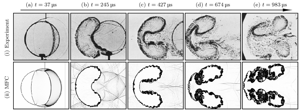
Figure 1: Comparison between (i) experimental shadowgraphs of Haas and Sturtevant [80] and (ii) numerical schlieren visualizations [84] using MFC at select times (a)–(e) as labeled. Experimental images are ©Cambridge University Press 1987.

Visualizations of the shock impinging the bubble and subsequent breakup and vortex ring production are shown in figure 1. We see that the simulation results qualitatively match those of the experiment. Importantly, no spurious oscillations can be seen in the numerical schlieren images, despite their sensitivity to small density differences. We quantitatively compare our results to the experiment by considering the velocity of key flow features: Haas and Sturtevant [80] measured the velocity of the incident, reflected, and transmitted shocks, as well as the up and down-stream interfaces and jets. Our simulation results are within 10% of the experiments for all cases and are generally within about 5% of the experimental means. Our results are also consistent with those computed independently via the level set [85] and diffuse-interface methods [86], including the Kelvin–Helmholtz instability that develops along the bubble interface (see figure 1 (b)–(e)).

5.2 Shock–droplet/cylinder interaction

We next consider air shocks interacting with liquid media in two and three dimensions. These problems are more computationally challenging, primarily due to the larger density ratio. The first case we analyze consists of a Mach $1.47$ shock impinging a $4.8\text{\,}\mathrm{mm}$ diameter liquid water cylinder. The simulation parameterization can be found in Meng and Colonius [15].

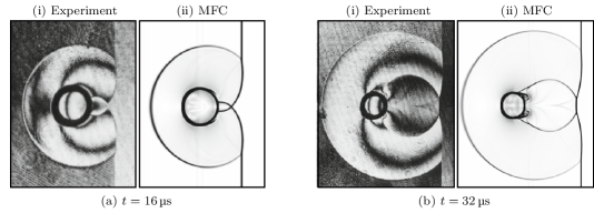
Figure 2: Comparison between (i) holographic interferograms [87] and (ii) numerical schlieren visualizations using MFC at select times (a) and (b) as labeled. The experimental images are reprinted from Igra and Takayama [87].

Figure 2 shows a visualization of experimental and our numerical results as the shock passes over the liquid cylinder. At early times it is difficult to assess the cylinder’s deformation, so we instead compare the primary and secondary waves that are generated. In figure 2 (a) we see that the primary wave system, including the incident and reflected shock, have the same locations for both experimental and numerical results. The secondary wave system is generated when the Mach stems on both sides of the cylinder converge to the rear stagnation point; in figure 2 (b) we see that these also match closely.

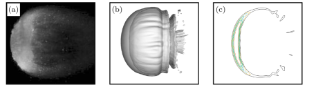
Figure 3: Comparison of (a) experimental [88] and (b) numerical water droplets isosurface $\alpha_{l}=0.01$. (c) shows isocontours of $\alpha_{l}$ ranging from $0.01$ to $0.99$.

We also consider the breakup of a spherical water droplet due to a helium shock (Mach $0.59$ observed in the post-shock flow), following the experimental conditions of Theofanous et al. [88]. A full exposition of the simulation conditions can be found in Meng and Colonius [14]. Figure 3 shows their experimental image and volume fraction isosurfaces and sliced isocontours from our simulations. We use a small $\alpha_{l}=0.01$ value for the isosurface of figure 3 (b) for comparison purposes since images from experiments are often obscured by the fine mist generated. While it is challenging to obtain accurate timing data from the experiments, a qualitative agreement between experiment and simulation are still observed for the shear-induced entrainment of the droplet.

5.3 Spherical bubble dynamics

Numerical simulation of cavitating spherical gas bubbles is challenging because mixture-region compressibility must be properly treated, discrete conservation must be enforced, and sphericity should be maintained in the presence of large density and pressure ratios. We consider a collapsing and rebounding air bubble in water at 10 times higher pressure as a test of the capabilities of MFC. Specific simulation specifications were presented in Schmidmayer et al. [55]; further, we include a guided description of the simulation setup for this problem in the example_cases/3D_sphbubcollapse directory of the MFC package (see table 1).

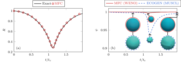
Figure 4: Evolution of (a) the dimensionless bubble radius $R$ and (b) its sphericity $\psi$. In (b) the nominal bubble shapes, represented by $\alpha_{l}=0.5$ isosurfaces, are shown at select times for MFC (WENO) and ECOGEN (MUSCL).

Figure 4 (a) shows the evolution of the bubble radius; it reaches a minimum near the nominal Rayleigh collapse time $t_{c}$ [89], then rebounds, as expected. The radius $R$ of our simulations is computed from the gas volume by assuming the shape is nearly spherical; this closely matches the solution expected following the Keller–Miksis equation [72]. We assess and compare the quality of our simulation with ECOGEN [54] via computation of the bubble sphericity during the collapse-rebound process. Figure 4 (b) shows this sphericity $\psi$ of the bubble, which is defined following Wadell [90] and a value of 1 indicates a spherical bubble. We see that the WENO scheme used by MFC can better maintain sphericity than a MUSCL scheme of ECOGEN formulated for the same diffuse-interface model [55], and is thus preferable for this problem.

5.4 Isentropic and Taylor–Green vortices

We next consider two- and three-dimension vortex problems as a means to verify our solutions of the flow equations. The two-dimension problem we consider is the evolution of a steady, inviscid, isentropic, ideal-gas vortex. This problem has been used previously to assess the convergence properties of high-order WENO schemes for smooth solutions to the Euler equations [49, 91]. We use it here to verify that we obtain high-order accuracy away from shocks and material interfaces; details regarding the numerical parameters and exact problem formulation can be found in Coralic and Colonius [41].

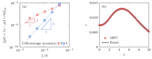
Figure 5: (a) $L_{\infty}$ density error associated with an isentropic steady vortex for the cell-averaged scheme accuracy labeled. (b) Non-dimensional kinetic energy dissipation rate $\varepsilon$ associated with the three-dimensional Taylor–Green vortex problem; the MFC solution is compared to the direct spectral solution of Brachet et al. [92].

Figure 5 (a) shows the density error for both low- and high-order finite volume cell-averaging (following section 4). Since the solution should be steady, the error is computed as the deviation from the initial condition after 1 dimensionless time unit as a function of the grid size, for which $N$ is the number of finite volumes in one spatial direction. The convergence is 2nd- and 5th-order accurate for 2nd- and 4th-order-accurate cell-averaging schemes, respectively. Thus, we conclude that for multi-dimensional problems the 4th-order-accurate cell averaging we employ is required to achieve 5th-order accuracy associated with the WENO reconstructions.

We use the three-dimensional Taylor–Green vortex problem of Brachet et al. [92] to study the production of small length scales, including vortex stretching and dissipation. The simulation parameters again follow from Coralic and Colonius [41]. Figure 5 (b) shows the dimensionless dissipation rate of the kinetic energy $\varepsilon$ in dimensionless time $t$, as computed over the entire computational domain. We see that the vortex stretching grows until $t\approx 5$, after which the effects of viscous dissipation begin to dominate. MFC results closely match those of the direct solution computed by Brachet et al. [92] using spectral methods.

5.5 Further verification

MFC has been verified using several other problems, including several one-dimensional test cases. For example, of great importance are the development of spurious oscillations at material interfaces, which can significantly pollute simulation quality. To determine if such oscillations appear when using our method, Coralic and Colonius [41] considered the advection of an isolated air–water interface at constant velocity in a periodic domain. It was shown that when conservative variables are reconstructed, the interface is corrupted by spurious oscillations and the pressures can even become negative. Whereas when primitive variables are reconstructed, their character is oscillation free for both velocity and pressure down to round off error.

It is also challenging to predict the correct position and speed of waves that emit from shock–interface interactions. While the shock–bubble interaction problem considered in section 5.1 showed that our method can approximate these quantities when comparing to experiments, it is helpful to consider a similar problem in one-dimension where exact solutions are available. Following Liu et al. [28], Coralic and Colonius [41] used the methods employed by MFC to analyze a Mach $8.96$ helium shock wave impinging an air interface. It was shown that the numerical results quantitatively matches the associated exact solution, correctly identifying the position and speed of all waves in the problem while avoiding any spurious oscillations. Of similar character is the gas–liquid shock tube problem of Cocchi et al. [93], which has been used as a model for underwater explosions. For this, Coralic and Colonius [41] also showed that the numerical solution matches the exact one and correctly identifies the position and speed of all waves.

Finally, the ensemble-averaged bubbly flow model introduced in section 3.3 was verified by simulating a weak acoustic pulse impinging a dilute bubble screen and comparing to the linearized bubble dynamic results of Commander and Prosperetti [94]. We saw that the measured phase speed and acoustic attenuation, computed via the method of Ando [71] and Bryngelson et al. [69], match the expected results. Further, Bryngelson et al. [69] showed that this method quantitatively matches the volume-averaged formulation of the same problem [95, 96].

6 Illustrative examples

6.1 Shock-bubble dynamics in a vessel phantom

We demonstrate the capabilities of MFC by first considering the shock-induced collapse of a gas bubble inside a deformable vessel. This is closely related to the vascular injury that can occur during shock-wave lithotripsy treatments [97, 41]. This problem is particularly challenging because it involves lareg density-, pressure-, and viscosity-ratios as well as components with significantly different equation of state parameters. Specifically, we consider a $20\text{\,}\mathrm{\SIUnitSymbolMicro m}$ diameter air bubble centered in a $26\text{\,}\mathrm{\SIUnitSymbolMicro m}$ diameter cylindrical vessel filled with water and surrounded by $10\%$ gelatin (see figure 6 (a)). The problem is initialized via a $40\text{\,}\mathrm{MPa}$ shock wave impinging the side of the vessel. Details on the specific numerical setup can be found in Coralic [98].

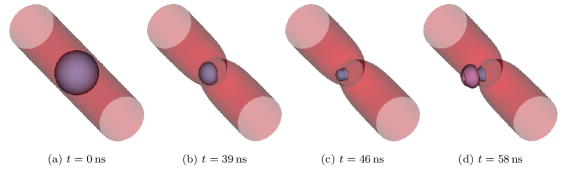
Figure 6: Temporal snapshots (a)–(d) that show the bubble collapse and vessel wall deformation. The shock impinges the vessel from right to left. The bubble and vessel walls are illustrated via their $0.5$ volume-fraction isosurfaces.

We visualize the bubble dynamics and subsequent impingement and deformation of the vessel in figure 6. We see that by $t=$39\text{\,}\mathrm{ns}$$ the bubble shape is asymmetric and the vessel contracts due to the incoming shock, after $t=$46\text{\,}\mathrm{ns}$$ the bubble surface has gained an inflection point and by $t=$66\text{\,}\mathrm{ns}$$ it impinges the vessel surface and becomes mushroom-shaped. Importantly, all surfaces remain smooth and free of spurious oscillations, despite the large density- and viscosity-ratios.

6.2 Vocalizing humpback whales

We next demonstrate the utility, flexibility, and robustness of the ensemble-averaged bubbly flow model described in section 3.3. For this, we model the humpback whale bubble-net feeding process [99]. Specifically, multiple humpback whales vocalize towards an annular bubbly region called a bubble net, which is modeled using the acoustic source terms of section 4.4 and bubbly regions described using the phase-averaged model.

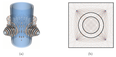
Figure 7: Visualizations of four model humpback whales vocalizing towards an annular bubble net in (a) three- and (b) two-dimensions. The acoustics are shown via isocontours of pressure and the annular bubble net is shaded.

We show the acoustics associated with the periodic excitation of the bubble net in figure 7 for both two- and three-dimensional configurations. In both cases, we see that the impedance associated with the relatively dilute bubble net (void fraction $10^{-4}$) effectively shields the core region from the vocalizations. Indeed, it is anticipated that the whales use their nets as a tool for corralling their prey into this relatively quiet, compact region. We also see that the curved material interfaces remain smooth and free of spurious oscillations.

7 Parallel performance benchmarks

It is important to ensure that our parallel implementation can utilize modern, large computer resources. To do this, we benchmark MFC’s parallel architecture via the usual scaling and speedup tests. These tests were carried out using 288 compute nodes, each containing two $2.6\text{\,}\mathrm{GHz}$ six-core AMD Opteron processors.

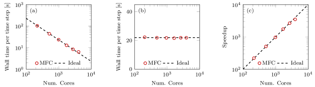
Figure 8: MFC performance benchmarks: (a) strong scaling, (b) weak scaling, and (c) speedup tests.

Figure 8 shows parallel performance benchmarks of MFC. The strong scaling test of figure 8 (a) measures how the solution time varies for a fixed problem size as the number of computing cores varies, the weak scaling test (figure 8 (b)) measures how well the computational load is balanced across the available cores by measuring solution time while fixing the grid size distributed to each core and varying the number of cores (thus changing the overall problem size), and the speedup test (figure 8 (c)) measures how the solution time increases with respect to serial computation as the number of cores varies. Thus, speedup is defined by the ratio of time cost of a parallel simulation with a certain of cores to a serial computation. The strong scaling and speedup tests are carried out on a $500^{3}$ grid, while a constant load of $50^{3}$ cells per core is maintained during the weak scaling test. For all tests, MFC performs very near the ideal threshold until the number of cores is $4096$, at which point the results deviate slightly from ideal.

8 Conclusions

We presented MFC, an open-source tool capable of simulating multi-component, multi-phase, and multi-scale flows. It uses state-of-the-art diffuse-interface models, coupled with high-order interface-capturing and Riemann solvers, to represent multi-material dynamics. MFC includes a variety of flow models and numerical methods, including spatial and temporal orders of accuracy, that are useful when considering the computational requirements of challenging open problems. It also includes options for additional physics and modeling techniques, including a sub-grid ensemble-averaged bubbly flow model.

We also described the requirements to build MFC and its design. This included external open-source software libraries that are readily available online. MFC was divided into three main components that initialize and simulate the flow, then process the exported simulation data. Each of these components is modular, and thus can be readily modified by new developers. They are coupled together via an intuitive input Python script that automatically generates the required Fortran input files and executes the software component. The exported simulation files can be readily analyzed or treated via parallel post-processing.

Finally, we presented a comprehensive set of validations, verifications, and illustrative examples. Validation was performed via comparisons to expected bubble dynamics and shock-bubble, shock-droplet, shock-water-cylinder experiments, while verification was obtained via numerical experiments involving isentropic and Taylor–Green vortices, as well as advected- and interface-interaction problems. The capabilities and fidelity of MFC were also illustrated using challenging studies of shock–bubble-viscous-vessel-wall interaction in application to shock-wave lithotripsy and acoustic-bubble-net dynamics in application to feeding humpback whales. A set of performance benchmarks also showed that MFC was able to perform near the ideal threshold of parallel computational efficiency.

References

References

- Brennen [2015] C. E. Brennen, Cavitation in medicine, Interface Focus 5 (2015).
- Laksari et al. [2015] K. Laksari, S. Assari, B. Seibold, K. Sadeghipour, K. Darvish, Computational simulation of the mechanical response of brain tissue under blast loading, Biomech. Model. Mechanobiol. 14 (2015) 459–472.
- Proud et al. [2015] W. G. Proud, T.-T. N. Nguyen, C. Bo, B. J. Butler, R. L. Boddy, A. Williams, S. Masouros, K. Brown, The high-strain rate loading of structural biological materials, Metall. Mater. Trans. A 46 (2015) 4559–4566.
- Coleman et al. [1987] A. J. Coleman, J. E. Saunders, L. Crum, M. Dyson, Acoustic cavitation generated by an extracorporeal shockwave lithotripter, Ultrasound Med. Biol. 13 (1987) 69–76.
- Pishchalnikov et al. [2003] Y. A. Pishchalnikov, O. A. Sapozhnikov, M. R. Bailey, J. C. Williams, R. O. Cleveland, T. Colonius, L. A. Crum, A. P. Evan, J. A. McAteer, Cavitation bubble cluster activity in the breakage of kidney stones by lithotripter shockwaves, J. Endourol. 17 (2003) 435–446.
- Ikeda et al. [2006] T. Ikeda, S. Yoshizawa, T. Masakata, J. S. Allen, S. Takagi, N. Ohta, T. Kitamura, Y. Matsumoto, Cloud cavitation control for lithotripsy using high intensity focused ultrasound, Ultrasound Med. Biol. 32 (2006) 1383–1397.
- Saurel et al. [2008] R. Saurel, F. Petitpas, R. Abgrall, Modelling phase transition in metastable liquids: Application to cavitating and flashing flows., J. Fluid Mech. 607 (2008) 313–350.
- Petitpas et al. [2009] F. Petitpas, J. Massoni, R. Saurel, E. Lapebie, L. Munier, Diffuse interface models for high speed cavitating underwater systems, Int. J. Mult. Flow 35 (2009) 747–759.
- Pelanti and Shyue [2014] M. Pelanti, K.-M. Shyue, A mixture-energy-consistent six-equation two-phase numerical model for fluids with interfaces, cavitation and evaporation waves, J. Comp. Phys. 259 (2014).
- Etter [2013] P. C. Etter, Underwater acoustic modeling and simulation, CRC Press, 2013.
- Kedrinskii [1976] V. Kedrinskii, Negative pressure profile in cavitation zone at underwater explosion near free surface, Acta Astro. 3 (1976) 623–632.
- Streeter [1983] V. Streeter, Transient cavitating pipe flow, J. Hydraulic Eng. 109 (1983) 1407–1423.
- Weyler et al. [1971] M. Weyler, V. Streeter, P. Larsen, An investigation of the effect of cavitation bubbles on the momentum loss in transient pipe flow, J. Basic Eng. 93 (1971) 1–7.
- Meng and Colonius [2018] J. C. Meng, T. Colonius, Numerical simulation of the aerobreakup of a water droplet, J. Fluid Mech. 835 (2018) 1108–1135.
- Meng and Colonius [2015] J. C. Meng, T. Colonius, Numerical simulations of the early stages of high-speed droplet breakup, Shock waves 25 (2015) 399–414.
- Schmidmayer et al. [2017] K. Schmidmayer, F. Petitpas, E. Daniel, N. Favrie, S. L. Gavrilyuk, A model and numerical method for compressible flows with capillary effects, J. Comp. Phys. 334 (2017) 468–497.
- Engel [1958] O. G. Engel, Fragmentation of waterdrops in the zone behind an air shock, J. Res. Natl. Bur. Stand 60 (1958) 245–280.
- Joseph et al. [1999] D. D. Joseph, J. Belanger, G. Beavers, Breakup of a liquid drop suddenly exposed to a high-speed airstream, Int. J. Mult. Flow 25 (1999) 1263–1303.
- Chauvin et al. [2015] A. Chauvin, E. Daniel, A. Chinnayya, J. Massoni, G. Jourdan, Shock waves in sprays: numerical study of secondary atomization and experimental comparison, Shock waves 26 (2015) 403–415.
- Tagawa et al. [2013] Y. Tagawa, N. Oudalov, A. E. Ghalbzouri, C. Sun, D. Lohse, Needle-free injection into skin and soft matter with highly focused microjets, Lab Chip 13 (2013) 1357–1363.
- Veilleux [2019] J.-C. Veilleux, Pressure and stress transients in autoinjector devices, Ph.D. thesis, California Institute of Technology, 2019.
- Fuster [2018] D. Fuster, A review of models for bubble clusters in cavitating flows, Flow, Turbulence and Combustion (2018) 1–40.
- Ball et al. [2000] G. J. Ball, B. P. Howell, T. G. Leighton, M. Schofield, Shock-induced collapse of a cylindrical air cavity in water: a free-Lagrange simulation, Shock waves 10 (2000) 265–276.
- Turangan et al. [2017] C. K. Turangan, G. J. Ball, A. R. Jamaluddin, T. G. Leighton, Numerical studies of cavitation erosion on an elastic–plastic material caused by shock-induced bubble collapse, Proc. Royal Soc. A 473 (2017) 20170315.
- Glimm et al. [2003] J. Glimm, X. L. Li, Y. Liu, Z. L. Xu, N. Zhao, Conservative front tracking with improved accuracy, SIAM J. Numer. Anal. 41 (2003) 1926–1947.
- Cocchi and Saurel [1997] J. P. Cocchi, R. Saurel, A Riemann problem based method for the resolution of compressible multimaterial flows, J. Comp. Phys. 137 (1997) 265–298.
- Abgrall and Karni [2001] R. Abgrall, S. Karni, Computations of compressible multifluids, J. Comp. Phys. 169 (2001) 594–623.
- Liu et al. [2003] T. G. Liu, B. C. Khoo, K. S. Yeo, Ghost fluid method for strong shock impacting on material interface, J. Comp. Phys. 190 (2003) 651–681.
- Liu et al. [2011] W. Liu, L. Yuan, C. Shu, A conservative modification to the ghost fluid method for compressible multiphase flows, Commun. Comput. Phys. 10 (2011) 785–806.
- Pan et al. [2018] S. Pan, L. Han, X. Hu, N. A. Adams, A conservative interface-interaction method for compressible multi-material flows, J. Comp. Phys. 371 (2018) 870–895.
- Hu et al. [2006] X. Y. Hu, B. C. Khoo, N. A. Adams, F. L. Huang, A conservative interface method for compressible flows, J. Comp. Phys. 219 (2006) 553–578.
- Han et al. [2014] L. H. Han, X. Y. Hu, N. A. Adams, Adaptive multi-resolution method for compressible multi-phase flows with sharp interface model and pyramid data structure, J. Comp. Phys. 262 (2014) 131–152.
- Chang et al. [2013] C.-H. Chang, X. Deng, T. G. Theofanous, Direct numerical simulation of interfacial instabilities: a consistent, conservative, all-speed, sharp-interface method, J. Comp. Phys. 242 (2013) 946–990.
- Denner et al. [2018] F. Denner, C.-N. Xiao, B. G. M. van Wachem, Pressure-based algorithm for compressible interfacial flows with acoustically-conservative interface discretisation, J. Comp. Phys. 367 (2018) 192–234.
- Fuster and Popinet [2018] D. Fuster, S. Popinet, An all-Mach method for the simulation of bubble dynamics problems in the presence of surface tension, J. Comp. Phys. 374 (2018) 752–768.
- Mirjalili et al. [2018] S. Mirjalili, C. B. Ivey, A. Mani, Comparison between the diffuse interface and volume of fluid methods for simulating two-phase flows, arXiv preprint arXiv:1803.07245 (2018).
- Johnsen and Ham [2012] E. Johnsen, F. Ham, Preventing numerical errors generated by interface-capturing schemes in compressible multi-material flows, J. Comp. Phys. 231 (2012) 5705–5717.
- Perigaud and Saurel [2005] G. Perigaud, R. Saurel, A compressible flow model with capillary effects, J. Comp. Phys. 209 (2005) 139–178.
- Shyue [1999] K. M. Shyue, A fluid-mixture type algorithm for compressible multicomponent flow with van der waals equation of state, J. Comp. Phys. 456 (1999) 43–88.
- Johnsen and Colonius [2006] E. Johnsen, T. Colonius, Implementation of weno schemes in compressible multicomponent flow problems, J. Comp. Phys. 219 (2006) 715–732.
- Coralic and Colonius [2014] V. Coralic, T. Colonius, Finite-volume WENO scheme for viscous compressible multicomponent flow problems, J. Comp. Phys. 219 (2014) 715–732.
- Massoni et al. [2002] J. Massoni, R. Saurel, B. Nkonga, R. Abgrall, Some models and Eulerian methods for interface problems between compressible fluids with heat transfer, Int. J. Heat Mass Transfer 45 (2002) 1287–1307.
- Meng [2016] J. C. Meng, Numerical simulations of droplet aerobreakup, Ph.D. thesis, California Institute of Technology, 2016.
- Allaire et al. [2002] G. Allaire, S. Clerc, S. Kokh, A five-equation model for the simulation of interfaces between compressible fluids, J. Comp. Phys. 181 (2002) 577–616.
- Kapila et al. [2001] A. Kapila, R. Menikoff, J. Bdzil, S. Son, D. Stewart, Two-phase modeling of DDT in granular materials: Reduced equations, Phys. Fluids 13 (2001) 3002–3024.
- Saurel et al. [2009] R. Saurel, F. Petitpas, R. A. Berry, Simple and efficient relaxation methods for interfaces separating compressible fluids, cavitating flows and shocks in multiphase mixtures, J. Comp. Phys. 228 (2009) 1678–1712.
- Abgrall [1996] R. Abgrall, How to prevent pressure oscillations in multicomponent flow calculations: a quasi conservative approach, J. Comp. Phys. 125 (1996) 150–160.
- Jiang and Schu [1996] G. S. Jiang, C. W. Schu, Efficient implementation of weighted ENO schemes, J. Comp. Phys. 126 (1996) 202–228.
- Balsara and Shu [2000] D. S. Balsara, C. W. Shu, Monotonicity preserving weighted essentially non-oscillatory schemes with increasingly high order of accuracy, J. Comp. Phys. 160 (2000) 405–452.
- Henrick and an d J. M. Powers [2005] A. K. Henrick, T. D. A. an d J. M. Powers, Mapped weighted essentially non-oscillatory schemes: achieving optimal order near critical points, J. Comp. Phys. 207 (2005) 542–567.
- Toro [2009] E. Toro, Riemann Solvers and Numerical Methods for Fluid Dynamics: A Practical Introduction, Springer, Dordrecht, New York, 2009.
- Toro et al. [1994] E. Toro, M. Spruce, W. Speares, Restoration of the contact surface in the HLL-Riemann solver, Shock waves 4 (1994) 25–34.
- Gottlieb and Shu [1998] S. Gottlieb, C.-W. Shu, Total variation diminishing Runge–Kutta schemes, Math. Comput. 67 (1998) 73–85.
- Schmidmayer et al. [2018] K. Schmidmayer, A. Marty, F. Petitpas, E. Daniel, ECOGEN, an open-source tool dedicated to multiphase compressible multiphysics flows, in: 53rd 3AF Int. Conf. App. Aero., 2018.
- Schmidmayer et al. [2019] K. Schmidmayer, S. H. Bryngelson, T. Colonius, An assessment of multicomponent flow models and interface capturing schemes for spherical bubble dynamics, under review (2019).
- Weller et al. [1998] H. G. Weller, G. Tabor, H. Jasak, C. Fureby, A tensorial approach to computational continuum mechanics using object-oriented techniques, Comput. Phys. 12 (1998) 620–631.
- Frigo and Johnson [1998] M. Frigo, S. G. Johnson, FFTW: An adaptive software architecture for the FFT, in: Proc. 1998 IEEE Intl. Conf. Acoustics Speech and Signal Processing, volume 3, IEEE, 1998, pp. 1381–1384.
- Miller [2019] M. Miller, Silo–a mesh and field I/O library and scientific database, Lawrence Livermore National Laboratory (2019). URL: https://wci.llnl.gov/simulation/computer-codes/silo.
- Halbwachs et al. [1991] N. Halbwachs, P. Caspi, P. Raymond, D. Pilaud, The synchronous data flow programming language lustre, Proc. IEEE 79 (1991) 1305–1320.
- Childs et al. [2012] H. Childs, E. Brugger, B. Whitlock, J. Meredith, S. Ahern, D. Pugmire, K. Biagas, M. Miller, C. Harrison, G. H. Weber, H. Krishnan, T. Fogal, A. Sanderson, C. Garth, E. W. Bethel, D. Camp, O. Rübel, M. Durant, J. M. Favre, P. Navrátil, VisIt: An end-user tool for visualizing and analyzing very large data, in: High Performance Visualization–Enabling Extreme-Scale Scientific Insight, 2012, pp. 357–372.
- Ahrens et al. [2005] J. Ahrens, B. Geveci, C. Law, Paraview: An end-user tool for large data visualization, The Visualization Handboo 717 (2005).
- Menikoff and Plohr [1989] R. Menikoff, B. J. Plohr, The Riemann problem for fluid-flow of real materials, Rev. Mod. Phys. 61 (1989) 75–130.
- Le Métayer et al. [2004] O. Le Métayer, J. Massoni, R. Saurel, Elaborating equations of state of a liquid and its vapor for two-phase flow models, Int. J. Therm. Sci. 43 (2004) 265–276.
- Marsh [1980] S. P. Marsh, LASL Shock Hugoniot Data, Los Alamos Series on Dynamic Material Properties, University of California Press, Berkeley, 1980.
- Gojani et al. [2009] A. B. Gojani, K. Ohtani, K. Takayama, S. H. R. Hosseini, Shock Hugoniot and equations of states of water, castor oil, and aqueous solutions of sodium chloride, sucrose and gelatin, Shock waves 26 (2009) 63–68.
- Wood [1930] A. B. Wood, A textbook of sound, G. Bell and Sons LTD, London (1930).
- Wallis [1969] G. B. Wallis, One-dimensional two-phase flow, McGraw-Hill, 1969.
- Zhang and Prosperetti [1994] D. Z. Zhang, A. Prosperetti, Ensemble phase-averaged equations for bubbly flows, Phys. Fluids 6 (1994).
- Bryngelson et al. [2019] S. H. Bryngelson, K. Schmidmayer, T. Colonius, A quantitative comparison of phase-averaged models for bubbly, cavitating flows, Int. J. Mult. Flow 115 (2019) 137–143.
- Colonius et al. [2008] T. Colonius, R. Hagmeijer, K. Ando, C. E. Brennen, Statistical equilibrium of bubble oscillations in dilute bubbly flows, Phys. Fluids 20 (2008).
- Ando [2010] K. Ando, Effects of polydispersity in bubbly flows, Ph.D. thesis, California Institute of Technology, 2010.
- Keller and Miksis [1980] J. B. Keller, M. Miksis, Bubble oscillations of large amplitude, J. Acoustic. Soc. Am. 68 (1980).
- Preston et al. [2007] A. Preston, T. Colonius, C. E. Brennen, A reduced-order model of diffusion effects on the dynamics of bubbles, Phys. Fluids 19 (2007).
- Meng [2016] J. C. Meng, Numerical simulations of droplet aerobreakup, Ph.D. thesis, California Institute of Technology, 2016.
- Li [2003] S. Li, WENO schemes for cylindrical and spherical geometry, Technical Report Los Alamos Report LA-UR-03-8922, Los Alamos National Laboratory, Los Alamos, NM, 2003.
- Mignone [2014] A. Mignone, High-order conservative reconstruction schemes for finite volume methods in cylindrical and spherical coordinates, J. Comp. Phys. 270 (2014) 784–814.
- Wang and Johnsen [2013] S. Wang, E. Johnsen, High-order schemes for cylindrical/spherical geometries with cylindrical/spherical symmetry, in: 21st AIAA Computational Fluid Dynamics Conference, AIAA 2013-2430, San Diego, CA, 2013.
- Mohseni and Colonius [2000] K. Mohseni, T. Colonius, Numerical treatment of polar coordinate singularities, J. Comp. Phys. 157 (2000) 787–795.
- Maeda and Colonius [2017] K. Maeda, T. Colonius, A source term approach for generation of one-way acoustic waves in the Euler and Navier–Stokes equations, Wave Motion 75 (2017) 36–49.
- Haas and Sturtevant [1987] J. F. Haas, B. Sturtevant, Interaction of weak shock waves with cylindrical and spherical gas inhomogeneities, J. Fluid Mech. 181 (1987) 41–76.
- Terashima and Tryggvason [2009] H. Terashima, G. Tryggvason, A front-tracking/ghost-fluid method for fluid interfaces in compressible flows, J. Comp. Phys. 228 (2009) 4012–4037.
- Fedkiw et al. [1999] R. P. Fedkiw, T. Aslam, B. Merriman, S. Osher, A non-oscillatory Eulerian approach to interfaces in multimaterial flows (the ghost fluid method), J. Comp. Phys. 152 (1999) 457–492.
- Hu and Khoo [2004] X. Y. Hu, B. C. Khoo, An interface interaction method for compressible multifluids, J. Comp. Phys. 198 (2004).
- Quirk and Karni [1996] J. J. Quirk, S. Karni, On the dynamics of a shock-bubble interaction, J. Fluid Mech. 318 (1996) 129–163.
- Hejazialhosseini et al. [2010] B. Hejazialhosseini, D. Rossinelli, M. Bergdorf, P. Koumoutsakos, High order finite volume methods on wavelet-adapted grids with local time-stepping on multicore architectures for the simulation of shock-bubble interactions, J. Comp. Phys. 229 (2010) 8364–8383.
- So et al. [2012] K. K. So, X. Y. Hu, N. A. Adams, Anti-diffusion interface sharpening technique for two-phase compressible flow simulations, J. Comp. Phys. 231 (2012) 4304–4323.
- Igra and Takayama [2001] D. Igra, K. Takayama, Numerical simulation of shock wave interaction with a water column, Shock waves 11 (2001) 219–228.
- Theofanous et al. [2012] T. G. Theofanous, V. V. Mitkin, C. L. Ng, C.-H. Chang, X. Deng, S. Sushchikh, The physics of aerobreakup. part II. Viscous liquids, Phys. Fluids 24 (2012) 022104.
- Brennen [1995] C. E. Brennen, Cavitation and bubble dynamics, Oxford University Press, 1995.
- Wadell [1935] H. Wadell, Volume, shape, and roundness of quartz particles, J. Geol. 43 (1935) 250–280.
- Titarev and Toro [2004] V. A. Titarev, E. F. Toro, Finite-volume WENO schemes for three-dimensional conservation laws, J. Comp. Phys. 201 (2004) 238–260.
- Brachet et al. [1983] M. E. Brachet, D. I. Meiron, S. A. Orszag, B. G. Nickel, R. H. Morf, U. Frisch, Small-scale structure of the Taylor–Green vortex, J. Fluid Mech. 130 (1983) 411–452.
- Cocchi et al. [1996] J. P. Cocchi, R. Saurel, J. C. Loraud, Treatment of interface problems with Godunov-type schemes, Shock waves 5 (1996) 347–357.
- Commander and Prosperetti [1989] K. W. Commander, A. Prosperetti, Linear pressure waves in bubbly liquids: Comparison between theory and experiments, J. Acoustic. Soc. Am. 85 (1989).
- Fuster and Colonius [2011] D. Fuster, T. Colonius, Modelling bubble clusters in compressible liquids, J. Fluid Mech. 688 (2011) 352–389.
- Maeda and Colonius [2018] K. Maeda, T. Colonius, Eulerian–Lagrangian method for simulation of cloud cavitation, J. Comp. Phys. 371 (2018) 994–1017.
- Coralic and Colonius [2013] V. Coralic, T. Colonius, Shock-induced collapse of a bubble inside a deformable vessel, Eur. J. Mech.–B/Fluids 40 (2013) 64–74.
- Coralic [2015] V. Coralic, Simulation of shock-induced bubble collapse with application to vascular injury in shockwave lithotripsy, Ph.D. thesis, California Institute of Technology, 2015.
- Hain et al. [1982] J. H. W. Hain, G. R. Carter, S. D. Kraus, C. A. Mayo, H. E. Winn, Feeding behavior of the humpback whale, megaptera novaeangliae, in the western north Atlantic, Fishery Bull. 8 (1982) 259–268.